Masses of excited baryons from chirally improved quenched lattice QCD

Abstract

Whereas ground state spectroscopy for quenched QCD is well understood, it is still a challenge to obtain results for excited hadron states. In our study we present results from a new approach for determining spatially optimized operators for lattice spectroscopy of excited hadrons. In order to be able to approach physical quark masses we work with the chirally improved Dirac operator, i.e., approximate Ginsparg-Wilson fermions. Since these are computationally expensive we restrict ourselves to a few quark sources. We use Jacobi smeared quark sources with different widths and combine them to construct hadron operators with different spatial wave functions. This allows us to identify the Roper state and other excited baryons, also in the strange sector.

1 Quark sources and interpolating fields

Ground state spectroscopy on the lattice is by now a well understood physical problem with impressive agreement with experiment. The lattice study of excited states is not as advanced. The Euclidean correlation function of an interpolating operator contains contributions from all states with the correct quantum numbers and the masses of the excited states show up only in the sub-leading exponentials. A direct fit to a sum of exponentials is cumbersome since the signal is strongly dominated by the ground state. Also with methods such as constrained fits, the maximum entropy method [1, 2] and a recently proposed method [3] one still needs high statistics for reliable results.

An alternative method is the variational method [4] where one diagonalizes a matrix containing all cross-correlations of a set of several basis operators $O_{i}$ with the correct quantum numbers,

$$C(t)_{ij}=\langle O_{i}(t)\,O_{j}^{\dagger}(0)\rangle=\sum_{n}\;\langle 0|O_{i}|n\rangle e^{-t\,M_{n}}\langle n|O_{j}^{\dagger}|0\rangle\;,$$ (1)

(written here for infinite temporal extent of the lattice and operators projected to vanishing spatial momentum). For a large enough and properly chosen set of basis operators each eigenmode is then dominated by a different physical state. Finding these states is equivalent to solving the generalized eigenvalue problem [4] with eigenvalues behaving as

$$\lambda^{(k)}(t)\propto e^{-t\,M_{k}}\left[1+{\cal O}(e^{-t\Delta M_{k}})\right]\;.$$ (2)

Each eigenvalue corresponds to a different energy level $M_{k}$ dominating its exponential decay; $\Delta M_{k}$ is the distance to nearby energy levels. The optimal operators which have maximal overlap with the physical states are linear combinations of the basis operators. After normalization the largest eigenvalue gives the correlator of the ground state, the second-largest eigenvalue corresponds to the first excited state, and so on.

Although the set of basis operators can be made arbitrarily large, in realistic calculations the intrinsic statistical errors make the diagonalization increasingly unstable. The challenge is then to provide a set of operators large enough to span the physically relevant space but still small enough to allow significant results for the given statistics.

In earlier work [5] we used three different interpolating fields for the nucleon sector, but could not resolve a signal for the Roper excitation. Here we concentrate on the first two of those,

$$\chi_{1}(x)=\epsilon_{abc}\left[u_{a}^{T}(x)\,C\,\gamma_{5}\,d_{b}(x)\right]u_{c}(x)\;,\quad\chi_{2}(x)=\epsilon_{abc}\left[u_{a}^{T}(x)\,C\,d_{b}(x)\right]\gamma_{5}\,u_{c}(x)\;.$$ (3)

We concluded that in order to get a reliable Roper signal it is also important to optimize the spatial properties of the interpolating operators. It can be argued that a node in the radial wave function is necessary to capture reliably the Roper state or other radially excited hadrons. In [6] we demonstrated that an elegant solution is to combine Jacobi smeared quark sources with different widths to build the hadron operators and compute the cross-correlations in the variational method. We find good effective mass plateaus for the first and partly the second and even the third radially excited states. The eigenvalues $\lambda^{(k)}(t)$ are then fitted using standard techniques.

Already earlier [7] Jacobi smeared sources were combined with point sources and cross-correlations studied in similar spirit (see also [8]). The technique of Jacobi smearing is well known [7, 9]. The smeared source lives in the timeslice $t=0$ and is constructed by iterated multiplication with a smearing operator $H$ on a point-like source. The operator $H$ is the spatial hopping part of the Wilson term at timeslice 0; it is trivial in Dirac space and acts only on the color indices. This construction has two free parameters: The number of smearing steps $N$ and the hopping parameter $\kappa$. These can be used to adjust the profile of the source. We worked with two different sources, a narrow source $n$ and a wide source $w$ with parameters chosen such that the profiles approximate Gaussian distributions [6]. The distribution of the two source-types correspond to half-widths of $\sigma\approx 0.27$ fm and $\sigma\approx 0.41$ fm.

The two sources allow the system to build up radial wave functions with and without a node. The parameters were chosen such that simple linear combinations $c_{n}\,n\,+\,c_{w}\,w$ of the narrow and wide profile can approximate the first and second radial wave functions of the spherical harmonic oscillator: The coefficients $c_{n}\sim 0.6,c_{w}\sim 0.4$ approximate a Gaussian with a half-width of $\sigma\sim 0.33$ fm, while $c_{n}\sim 2.2,c_{w}\sim-1.2$ approximate the corresponding excited wave function with one node. Note, however, that the final contribution of the corresponding source terms is not pre-determined but results from the diagonalization.

Following the variational method [4] we compute the complete correlation matrix of operators. The hadron sources we use for the correlation matrix are constructed from the narrow and wide quark sources. Respecting symmetries we then have for both types of nucleon operators (3) six combinations of wide or narrow quark sources, in total 12 interpolating field operators and a $12\times 12$ correlation matrix. The final form of the wave function is determined through the eigenvectors resulting from the variational method.

2 Baryon results

We use the chirally improved Dirac operator [10] and work in the quenched limit, ie., without dynamical fermions. This operator is an approximate Ginsparg-Wilson operator and was well tested in quenched ground state spectroscopy [11] where pion masses down to 250 MeV have been reached at a considerably smaller numerical cost than needed for exact Ginsparg-Wilson fermions. The gauge configurations were generated on a $12^{3}\times 24$ lattice with the Lüscher-Weisz action [12] (further studies for larger lattices are in progress). The inverse gauge coupling is $\beta=7.9$, giving rise to a lattice spacing of $a=0.148(2)$ fm as determined from the Sommer parameter [13]. The statistics of our ensemble is 100 configurations. For the $u$, $d$ quarks we use degenerate quark masses $m$ ranging from $a\,m=0.02$ to $a\,m=0.20$. More details are discussed in [6].

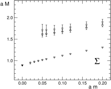
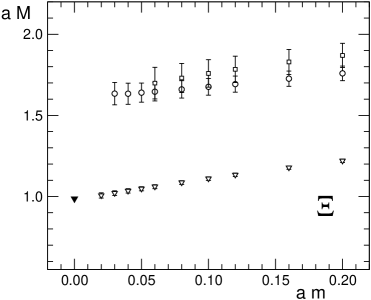
Figure 1: Masses of $\Sigma$ and $\Xi$ baryons in units of the lattice spacing $a\approx 0.148$ fm (=1/1.33 GeV) (triangles: ground state, circles: negative parity ground state, squares: first positive parity excited state, full symbol: experimental value of ground state); the mass of the strange quark has been adjusted to give physical $K$-meson mass.

Although we determine the full correlation matrix as discussed, it turns out to be numerically advantageous to analyze only a subset of operators. The exponential decay of the three leading eigenvalues is clearly identified. We identify these signals with the nucleon, the Roper state and the next positive parity resonance $N(1710)$. The larger eigenvalues have too large statistical errors for a reliable interpretation (see also [1] concerning the problem of nucleon-$\eta^{\prime}$ ghost contributions).

In principle both interpolators $\chi_{1}$ and $\chi_{2}$ should couple to all states with the corresponding quantum numbers; however, the coupling amplitude depends on the internal structure of the physical states (with possibly different overlap). Since we can continuously increase the quark mass and thus make contact with the heavy quark region we also may argue in such a framework. All Roper states form an excited 56-plet of SU(6) and in this multiplet the parity of any two-quark subsystem is positive. The $N(1710)$ belongs to another multiplet containing both positive and negative parity two-quark subsystems. The two-quark subsystem in the brackets in $\chi_{1}$ has positive parity, while the subsystem in the brackets of $\chi_{2}$ has negative parity. Hence in $\chi_{2}$ we should see only the signal from the $N(1710)$ state, and no signals from the nucleon and the Roper. This is exactly what we observe in [6], where the relevant figures for the nucleon channel are shown.

We may also combine quarks with different masses, allowing for a strange quark. We fix the strange quark mass such that the $K$-meson mass has its experimental value in the chiral limit of the $u,\,d$-masses. We then can determine also the $\Sigma$- and $\Xi$-baryons using interpolator $\chi_{1}$ and again different width quarks sources. First results are exhibited in Fig. 1. We have to stress, however, that the results given here are for relatively small lattices (spatial lattice size 1.8 fm).

A crucial test of our method is to check whether indeed the ground state is built from a nodeless combination of our sources and the excited states do show nodes. This question can be addressed by analyzing the eigenvectors of the correlation matrix. This has been done in [6] and indeed confirms the expectation.

3 Conclusion

Ground state masses approach, in naive chiral extrapolation, their experimental values well. The excited state masses are above their experimental values. Since our results are for small spatial lattice size a volume dependence study still has to confirm this behavior. Excited states may be more affected by finite volume effects, but also be more sensitive to the quenched approximation. Finite volume studies, including also scaling properties, are under way.

References

- [1] N. Mathur et al., Phys. Lett. B 605 (2005) 137; hep-lat/0405001.
- [2] S. Sasaki, Prog. Theor. Phys. Suppl. 151 (2003) 143.
- [3] D. Guadagnoli, M. Papinutto and S. Simula, Phys. Lett. B 604 (2004) 74, and these proceedings.
- [4] C. Michael, Nucl. Phys. B 259 (1985) 58; M. Lüscher and U. Wolff, Nucl. Phys. B 339 (1990) 222.
- [5] D. Brömmel et al, Phys. Rev. D 69 (2004) 094513; Nucl. Phys. B Proc. Suppl. 129-130 (2004) 251.
- [6] T. Burch et al., Phys. Rev. D 70 (2004) 054502; see also hep-lat/0409014.
- [7] C.R. Allton et al. [UKQCD Collaboration], Phys. Rev. D 47 (1993) 5128.
- [8] T. Burch, C. Gattringer and A. Schäfer, hep-lat/0408038.
- [9] C. Best et al., Phys. Rev. D 56 (1997) 2743; C. Alexandrou et al., Nucl. Phys. B 414 (1994) 815.
- [10] C. Gattringer, Phys. Rev. D 63 (2001) 114501; C. Gattringer, I. Hip, C. B. Lang, Nucl. Phys. B 597 (2001) 451.
- [11] C. Gattringer et al. [BGR Collaboration], Nucl. Phys. B 677 (2004) 3; Nucl. Phys. B Proc. Suppl. 119 (2003) 796; C. Gattringer, Nucl. Phys. B Proc. Suppl. 119 (2003) 122.
- [12] M. Lüscher and P. Weisz, Commun. Math. Phys. 97 (1985) 59; G. Curci, P. Menotti and G. Paffuti, Phys. Lett. B 130 (1983) 205.
- [13] C. Gattringer, R. Hoffmann and S. Schaefer, Phys. Rev. D 65 (2002) 094503.