Relativistic effects in neutron-deuteron elastic scattering

Abstract

We solved the three-nucleon (3N) Faddeev equation including relativistic features at incoming neutron lab energies $E_{n}^{lab}=28$, $65$, $135$ and $250$ MeV. Those features are relativistic kinematics, boost effects and Wigner spin rotations. As dynamical input a relativistic nucleon-nucleon (NN) interaction exactly on-shell equivalent to the AV18 NN potential has been used. The effects of Wigner rotations for elastic scattering observables were found to be small. The boost effects are significant at higher energies. They diminish the transition matrix elements at higher energies and lead in spite of the increased relativistic phase-space factor as compared to the nonrelativistic one to rather small effects in the cross section, which are mostly restricted to the backward angles.

I Introduction

High precision nucleon-nucleon (NN) potentials such as AV18 AV18 , CDBonn CDBONN , Nijm I, II and 93 NIJMI describe the NN data set up to about 350 MeV very well. When these forces are used to predict binding energies of three-nucleon (3N) systems they underestimate the experimental bindings of ${}^{3}H$ and ${}^{3}He$ by about 0.5-1 MeV Friar1993 ; Nogga1997 . This missing binding energy can be cured by introducing a three-nucleon force (3NF) into the nuclear Hamiltonian Nogga1997 .

The study of elastic nucleon-deuteron (Nd) scattering and nucleon induced deuteron breakup revealed a number of cases where the nonrelativistic description based on pairwise forces only is insufficient to explain the data. Generally, the studied discrepancies between a theory based on NN potentials only and experiment become larger with increasing energy of the 3N system. Adding now a 3NF to the pairwise interactions leads in some cases to a better description of the data. The elastic Nd angular distribution in the region of its minimum and at backward angles is the best studied example wit98 ; sek02 . The clear discrepancy in this angular regions at energies below $\approx 100$ MeV nucleon lab energy between a theory based on NN potentials only and the cross section data can be removed by adding modern 3NFs to the nuclear Hamiltonian. Such a 3NF must be adjusted with each NN potential separately to the experimental binding of ${}^{3}H$ and ${}^{3}He$ wit98 ; wit01 ; sek02 . At energies higher than $\approx 100$ MeV current 3NFs only partially improve the description of cross section data and the remaining discrepancies, which increase with energy, indicate the possibility of relativistic effects. The need for a relativistic description of 3N scattering was also raised when precise measurements of the total cross section for neutron-deuteron (nd) scattering abf98 were analyzed within the framework of nonrelativistic Faddeev calculations wit99 . NN forces alone were insufficient to describe the data above $\approx 100$ MeV. The effects due to relativistic kinematics considered in ref. wit99 were comparable at higher energies to the effects due to 3NFs. These indications show the importance of a study taking relativistic effects in the 3N continuum into account.

The estimation of relativistic effects on the binding energy of three nucleons has been the focus of a lot of work. Basically two different aproaches have been followed: one is a manifestly covariant scheme linked to a field theoretical approach Rupp92 ; Sam98 ; stad97 , the other one is based on relativistic quantum mechanics formulated on spacelike hypersurfaces in Minkowski space bak52 ; foldy74 ; keister91 ; kei91 . Within the second scheme the relativistic Hamiltonian for on the mass shell particles consists of relativistic kinetic energies and two- and many-body interactions including their boost corrections, which are dictated by the Poincaré algebra bak52 ; foldy74 ; keister91 ; kei91 . The applications of these two types of approaches to the 3N bound state have led to contradictory results. In the approach based on field theory, relativistic effects increase the triton binding energy, while in the approach based on relativistic Hamiltonians they decrease the triton binding energy. This requires further insights which is beyond the scope of this paper.

Due to the increased complexity of 3N scattering calculations as compared to the bound state problem no results for the 3N continuum including relativity are available. In order to extend the Hamiltonian scheme in equal time formulation to 3N scattering one needs as a starting point the Lorentz boosted NN potential which generates the NN t matrix in a moving frame via a standard Lippmann-Schwinger equation. Such potentials have been worked out and applied to a 3N bound state in kam2002 . The results obtained supported the relativistic effects found before in a relativistic quantum mechanics approach relform . The starting point for a NN potential in an arbitrary moving frame is the interaction in the two-nucleon c.m. system, which enters a relativistic NN Schrödinger or Lippmann-Schwinger equation. It differs from the nonrelativistic Schrödinger equation just by the relativistic form for the kinetic energy. The current realistic NN potentials are defined and fitted in the context of the nonrelativistic Schrödinger equation. Up to now NN potentials refitted with the same accuracy in the framework of the relativistic NN Schrödinger equation do not exist. In kam2002 such refitting was omitted and an analytical scale transformation of momenta which relates NN potentials in the nonrelativistic and relativistic Schrödinger equations in such a way, that exactly the same NN phase shifts are obtained by both equations, was employed kam98 .

Though this transformation is not a substitute for a NN potential with proper relativistic features it can serve as a first step to illustrate the effects of Lorentz boosts on NN potentials. Such an approach was applied in kam2002 and we also will follow it in the present study to get the first estimation of relativistic effects in the 3N continuum. In this first study we would like to find out what are the changes of elastic nd scattering observables when the nonrelativistic form of the kinetic energy is replaced by the relativistic one and a proper treatment of boost effects and effects due to Wigner rotations of spin states is performed.

The paper is organized as follows. In Sec. II we lay out the relativistic features underlying our treatment for a relativized Faddeev equation in the 3N continuum. This incorporates the definition of the boosted two-body force, the various two-and three-body states in general frames, the Wigner rotations and the singularity structure of the relativistic free 3N propagator. Our manner to treat the 3N Faddeev equation is guided by the lines presented in  wit88 for the nonrelativistic case. In Sec. III we focus on the relativistic NN potential and discuss the quality of different approximations for the boosted potential. As a consequence, in this first study we restrict ourselves to the leading order relativistic term in the expansion of the boosted potential. In Sec. IV we apply our formulation based on a relativistic NN interaction which is exactly on-shell equivalent to the nonrelativistic AV18 potential and solve the relativized 3N Faddeev equation with different approximations for the boost. We show and discuss results for elastic Nd scattering. Sec. V contains a summary and outlook.

II Formulation

The nucleon-deuteron scattering with neutron and protons interacting through a NN potential $V$ alone is described in terms of a breakup operator T satisfying the Faddeev-type integral equation wit88 ; glo96

$$T|\phi> = tP|\phi>+tPG_{0}T|\phi>.$$ (1)

The two-nucleon (2N) t-matrix t results from the interaction $V$ through the Lippmann-Schwinger equation. The permutation operator $P=P_{12}P_{23}+P_{13}P_{23}$ is given in terms of the transposition $P_{ij}$ which interchanges nucleons i and j. The incoming state $|\phi>=|\vec{q}_{0}>|\phi_{d}>$ describes the free nucleon-deuteron motion with relative momentum $\vec{q}_{0}$ and the deuteron wave function $|\phi_{d}>$. Finally $G_{0}$ is the free 3N propagator. The physical picture underlying Eq.(1) is revealed after iteration which leads to a multiple scattering series for T.

The elastic nd scattering transition operator U is given in terms of T by wit88 ; glo96

$$U = PG_{0}^{-1}+PT.$$ (2)

This is our standard nonrelativistic formulation, which is equivalent to the nonrelativistic 3N Schrödinger equation plus boundary conditions. The formal structure of these equations in the relativistic case remains the same but the ingredients change. As explained in  relform the relativistic 3N Hamiltonian has the same form as the nonrelativistic one, only the momentum dependence of the kinetic energy changes and the relation of the pair interactions to the ones in their corresponding c.m. frames changes, too. Consequently all the formal steps leading to Eqs.(1) and (2) remain the same.

The relativistic kinetic energy of three equal mass nucleons in their c.m. system can conveniently be presented by introducing the free two-body mass operator. Let $\vec{k}$ and $-\vec{k}$ be the momenta in one of the two-body subsystems, then $2\omega({\vec{k}})\equiv 2\sqrt{m^{2}+{\vec{k}}^{\ 2}}$ is the momentum dependent 2N mass operator and the 3N kinetic energy can be written as

$$H_{0} = \sqrt{(2\omega({\vec{k}}))^{2}+{\vec{q}}^{\ 2}}+\sqrt{m^{2}+{\vec{q}}^{\ 2}},$$ (3)

where $\vec{q}$ is the momentum of the third particle and $-\vec{q}$ the total momentum of the chosen two-body subsystem (m is the nucleon mass). Any two-body subsystem can be chosen. As introduced in  relform1 the pair forces in the relativistic 3N Hamiltonian living in moving frames are chosen as

$$V(\vec{q}\,)\equiv\sqrt{(2\omega(\vec{k})+v)^{2}+{\vec{q}}^{\ 2}}-\sqrt{(2\omega(\vec{k}))^{2}+{\vec{q}}^{\ 2}},$$ (4)

where $V(\vec{q})$ for $\vec{q}=0$ reduces to the potential $v$ defined in the 2N c.m. system. Note that also in that system the relativistic kinetic energy of the two nucleons has to be chosen, which together with $v$ defines the interacting two-nucleon mass operator occuring in Eq.(4).

Let us now firstly regard the 2N subsystem. The standard nonrelativistic 2N Lippmann Schwinger equation turns now into a relativistic one, which in a general frame reads

$$t(\vec{k},\vec{k}~{}^{\prime};\vec{q}~{}) = V(\vec{k},\vec{k}~{}^{\prime};\vec{q}~{})+\int d^{3}k^{\prime\prime}{{V(\vec{k},\vec{k}~{}^{\prime\prime};\vec{q}~{})t(\vec{k}~{}^{\prime\prime},\vec{k}~{}^{\prime};\vec{q}~{})}\over{\sqrt{{(2\omega({\vec{k}}^{\ {}^{\prime}})^{\ 2}+{\vec{q}}^{\ 2}}}-\sqrt{{(2\omega({\vec{k}}^{\ {}^{\prime\prime}})^{\ 2}+{\vec{q}}^{\ 2}}}+i\epsilon}}.$$ (5)

We refer to $t(\vec{k},\vec{k}~{}^{\prime};\vec{q}~{})$ as the boosted 2N t-matrix like we talk of the boosted 2N potential in Eq.(4).

Using (4) the relativistic 2N Schrödinger equation for the deuteron in a moving frame can be cast into the form

$$\phi_{d}(\vec{k}) = {{1}\over{\sqrt{{M_{d}^{2}+{\vec{q}}^{\ 2}_{0}}}-\sqrt{{(2\omega(\vec{k}))^{2}+{\vec{q}}^{\ 2}_{0}}}}}\int d^{3}k^{\prime}V(\vec{k},\vec{k}~{}^{\prime};\vec{q}_{0})\phi_{d}(\vec{k}~{}^{\prime}),$$ (6)

where $\sqrt{{M_{d}^{2}+{\vec{q}}^{\ 2}_{0}}}$ is the energy of the deuteron in motion and $M_{d}$ its rest mass. This equation is a good check for the correct numerical implementation of the boosted potential $V(\vec{q})$ as will be used below.

The new relativistic ingredients in Eqs.(1) and (2) will therefore be the boosted t-operator and the relativistic 3N propagator

$$G_{0} = {{1}\over{E+i\epsilon-H_{0}}},$$ (7)

where $H_{0}$ is given in Eq. (3) and $E$ is the total 3N c.m. energy expressed in terms of the initial neutron momentum $\vec{q}_{0}$ relative to the deuteron

$$E = \sqrt{(M_{d})^{2}+{\vec{q}}_{0}^{\ 2}}+\sqrt{m^{2}+{\vec{q}}_{0}^{\ 2}}.$$ (8)

Currently Eq.(1) in its nonrelativistic form is numerically solved for any NN interaction using a momentum space partial wave decomposition. Details are presented in ref. wit88 . This turns Eq.(1) into a coupled set of two- dimensional integral equations. As we show now, in the relativistic case we can keep the same formal structure, though the kinematics and the momentum representation of the permutation operator P is more complex and boosted t-operators as well as Wigner rotations will appear.

In the nonrelativistic case the partial wave projected momentum space basis is

$$|pq(ls)j(\lambda{1\over{2}})IJ(t{1\over{2}})T>,$$ (9)

where p and q are the magnitudes of standard Jacobi momenta (see book ) and $(ls)j$ two-body quantum numbers with obvious meaning, $(\lambda 1/2)I$ refer to the third nucleon (described by the momentum q), $J$ is the total 3N angular momentum and the rest are isospin quantum numbers. This is now to be generalized to the relativistic case.

We regard firstly the two-nucleon system and replace the nonrelativistic relative two-nucleon momentum $\vec{p}$ by $\vec{k}$, where $\vec{k}$ and $-\vec{k}$ are related to general momenta of two nucleons, say $\vec{p}_{2}$ and $\vec{p}_{3}$, by a Lorentz boost:

$$\vec{k} \equiv \vec{k}(\vec{p}_{2},\vec{p}_{3})$$ (10)

$$= {1\over{2}}(\vec{p}_{2}-\vec{p}_{3}-\vec{p}_{23}{{E_{2}-E_{3}}\over{E_{23}+\sqrt{E_{23}^{2}-\vec{p}_{23}^{~{}2}}}}),$$ (11)

with $E_{i}=\sqrt{m^{2}+{\vec{p}}_{i}^{\ 2}}$, $E_{23}=E_{2}+E_{3}$ and $\vec{p}_{23}=\vec{p}_{2}+\vec{p}_{3}$. This is a relativistic generalization of the nonrelativistic relative momentum $\vec{p}$.

The individual momentum state with momentum $\vec{k}$ for an on-the-mass-shell particle with mass $m$ is defined in terms of the state in the rest frame as  kei91 ; Weinberg

$$U(\beta(k))|\vec{0}\mu> = \sqrt{{\omega_{m}({\vec{k}})\over{m}}}|\vec{k}\mu>.$$ (12)

Here $U(\beta(k))$ is the unitary operator related to the special (along $\vec{k}$) boost matrix $\beta(k)$, $\mu$ the spin magnetic quantum number and $k=(\omega_{m}({\vec{k}}),{\vec{k}})$ with $\omega_{m}({\vec{k}})=\sqrt{m^{2}+{\vec{k}}^{\ 2}}$. Note that by definition $\mu$ does not change. The $4\times 4$ matrix $\beta(k)$ is given in the Appendix.

A following unitary operation related to the general boost $\Lambda$ leads to the well known Wigner rotation  kei91 ; Weinberg :

$$U(\Lambda)|\vec{k}\mu> = \sqrt{{{m}\over{\omega_{m}({\vec{k}})}}}U(\Lambda)U(\beta(k))|\vec{0}\mu>$$ (13)

$$= U(\beta(k^{\prime}))U(\beta^{-1}(k^{\prime})\Lambda\beta(k))|\vec{0}\mu>\sqrt{{{m}\over{\omega_{m}({\vec{k}})}}}.$$ (14)

The argument in the second unitary operator is a rotation matrix

$$R(\Lambda,{\vec{k}}) \equiv \beta^{-1}(k^{\prime})\Lambda\beta(k)$$ (15)

and often denoted as Wigner rotation. Further the on shell momenta $k$ and $k^{\prime}$ are related by $k^{\prime}=\Lambda k$.

$R(\Lambda,{\vec{k}})$ being a rotation yields

$$U(\Lambda)|\vec{k}\mu> = U(\beta(k^{\prime}))\sum_{\mu^{\prime}}D^{{1\over{2}}}_{\mu^{\prime}\mu}(R(\Lambda,{\vec{k}}))|\vec{0}\mu^{\prime}>\sqrt{{{m}\over{\omega_{m}({\vec{k}})}}},$$ (16)

and using (12) again to

$$U(\Lambda)|\vec{k}\mu> = \sqrt{{\omega_{m}({\vec{k}}^{\ \prime})\over{\omega_{m}({\vec{k}})}}}\sum_{\mu^{\prime}}D^{{1\over{2}}}_{\mu^{\prime}\mu}(R(\Lambda,{\vec{k}}))|\vec{k}~{}^{\prime}\mu^{\prime}>.$$ (17)

Here $D^{{1\over{2}}}_{\mu^{\prime}\mu}$ are the standard SU(2) Wigner D-matrices rose and their arguments Euler angles which are related to $R$ as shown below.

Now we apply a general boost to the noninteracting two nucleon state

$$|\vec{k};\vec{0}\mu_{2}\mu_{3}> \equiv |\vec{k}\mu_{2},-\vec{k}\mu_{3}>.$$ (18)

In the notation to the left we changed from the two individual momenta to the relative momentum $\vec{k}$ and the total two-nucleon momentum zero. Since the two nucleons are noninteracting $U(\Lambda)$ acting on a two-body system is a tensor product

$$U(\Lambda) = U_{2}(\Lambda)U_{3}(\Lambda)$$ (19)

acting on the two spaces of nucleons 2 and 3. We choose $\Lambda$ as $\beta(P)$, where $P=(P_{0},\vec{P})\equiv(\omega_{m}({\vec{p}}_{2})+\omega_{m}({\vec{p}}_{3}),\vec{p}_{2}+\vec{p}_{3})$. That boost matrix $\beta(P)$ maps $\vec{k}$ into $\vec{p}_{2}$ and $-\vec{k}$ into $\vec{p}_{3}$. We obtain

$$U(\beta(P))|\vec{k};\vec{0}\mu_{2}\mu_{3}>\equiv U_{2}(\beta(P))|\vec{k}\mu_{2}>U_{3}(\beta(P))|-\vec{k}\mu_{3}>$$ (20)

$$\sqrt{{\omega_{m}({\vec{p}}_{2})\over{\omega_{m}({\vec{k}})}}}\sum_{\mu_{2}^{\prime}}D^{{1\over{2}}}_{\mu_{2}^{\prime}\mu_{2}}(R(\beta(P),\vec{k}))|\vec{p}_{2}\mu_{2}^{\prime}>\sqrt{{\omega_{m}({\vec{p}}_{3})\over{\omega_{m}({\vec{k}})}}}\sum_{\mu_{3}^{\prime}}D^{{1\over{2}}}_{\mu_{3}^{\prime}\mu_{3}}(R(\beta(P),-\vec{k}))|\vec{p}_{3}\mu_{3}^{\prime}>.$$ (21)

Of course $\vec{p}_{2}$ and $\vec{p}_{3}$ are given by the inverse relation to (10) and the related expression for $-\vec{k}$.

On the other hand the noninteracting two-nucleon system with total momentum zero can be considered as one object with a mass $M_{0}=2\omega_{m}({\vec{k}})$ and therefore according to the general relation (12) one obtains

$$U(\beta(P))|\vec{k};\vec{0}\mu_{2}\mu_{3}> = \sqrt{{\omega_{M_{0}}(\vec{P})\over{M_{0}}}}|\vec{k};\vec{P}\mu_{2}\mu_{3}>,$$ (22)

and we end up with

$$|\vec{k};\vec{P}\mu_{2}\mu_{3}> = |~{}{{\partial(\vec{p}_{2}~{}\vec{p}_{3})}\over{\partial(\vec{P}~{}\vec{k})}}~{}|^{1\over{2}}\sum_{\mu_{2}^{\prime}}D^{{1\over{2}}}_{\mu_{2}^{\prime}\mu_{2}}(R(\beta(P),\vec{k}))$$ (23)

$$\times \sum_{\mu_{3}^{\prime}}D^{{1\over{2}}}_{\mu_{3}^{\prime}\mu_{3}}(R(\beta(P),-\vec{k}))|\vec{p}_{2}\mu_{2}^{\prime}\vec{p}_{3}\mu_{3}^{\prime}>,$$ (24)

where

$$|~{}{{\partial(\vec{p}_{2}~{}\vec{p}_{2})}\over{\partial(\vec{P}~{}\vec{k})}}~{}| = {M_{0}\over{\omega_{M_{0}}(\vec{P})}}~{}{\omega_{m}(\vec{p}_{2})\over{\omega_{m}(\vec{k})}}~{}{\omega_{m}(\vec{p}_{3})\over{\omega_{m}(\vec{k})}}\equiv N^{2}({\vec{p}}_{2},{\vec{p}}_{3})$$ (25)

is the Jacobian for the Lorentz transformation from $(\vec{p}_{2},\vec{p}_{3})$ to $(\vec{P},\vec{k})$.

This relation generalizes the one used in relform and kam2002 from the spinless case to the one with spin. In the nonrelativistic case the D-matrices reduce to Kronecker symbols and the Jacobian is one. Thus $|\vec{p}_{2}\vec{p}_{3}\mu_{2}\mu_{3}>$ equals directly $|\vec{k}\vec{P}\mu_{2}\mu_{3}>$, where $\vec{k}$ equals the nonrelativistic relative momentum.

The next step is the transition to partial waves. Firstly one defines the two-body orbital angular momentum states

$$|k~{}l;\vec{0}\mu_{l}\mu_{2}\mu_{3}> \equiv \int d\hat{k}Y^{l}_{\mu_{l}}(\hat{k})|\vec{k};\vec{0}\mu_{2}\mu_{3}>.$$ (26)

Then we couple with the total spin $s$ in the two-nucleon c.m. system to the total angular momentum $j$ and its magnetic quantum number $\mu$:

$$|(ls)jk\mu;\vec{0}> \equiv \sum_{\mu_{2}\mu_{3}}\sum_{\mu_{s}\mu_{l}}({1\over{2}}\mu_{2}{1\over{2}}\mu_{3}|s\mu_{s})(l\mu_{l}s\mu_{s}|j\mu)|kl\mu_{l}\mu_{2}\mu_{3};\vec{0}>.$$ (27)

The special boost $\beta(P)$ leads then to

$$U(\beta(P))|(ls)jk\mu;\vec{0}> = \sqrt{{\omega_{M_{0}}(\vec{P})\over{M_{0}}}}|(ls)jk\mu;\vec{P}>$$ (28)

and applied individually leads finally to

$$|(ls)jk\mu;\vec{P}> = |~{}{{\partial(\vec{p}_{2}~{}\vec{p}_{3})}\over{\partial(\vec{P}~{}\vec{k})}}~{}|^{1\over{2}}\sum_{\mu_{2}\mu_{3}}\sum_{\mu_{s}\mu_{l}}({1\over{2}}\mu_{2}{1\over{2}}\mu_{3}|s\mu_{s})(l\mu_{l}s\mu_{s}|j\mu)\int d\hat{k}Y^{l}_{\mu_{l}}(\hat{k})$$ (29)

$$\times \sum_{\mu_{2}^{\prime}}D^{{1\over{2}}}_{\mu_{2}^{\prime}\mu_{2}}(R(\beta(P),\vec{k}))\sum_{\mu_{3}^{\prime}}D^{{1\over{2}}}_{\mu_{3}^{\prime}\mu_{3}}(R(\beta(P),-\vec{k}))|\vec{p}_{2}\mu_{2}^{\prime}\vec{p}_{3}\mu_{3}^{\prime}>.$$ (30)

This is the connection of the partial wave projected two-nucleon state with internal momentum k and total momentum $\vec{P}$ to arbitrary individual momentum and spin states.

Another requisite is the determination of the Euler angles ($\alpha,\beta,\gamma$) in the spin 1/2 D-matrices. According to (13) the two $4\times 4$ matrices

$$R(\beta(P),\vec{k}) = \beta^{-1}(p_{2})\beta(P)\beta(\omega_{m}({\vec{k}}),\vec{k})$$ (31)

$$R(\beta(P),-\vec{k}) = \beta^{-1}(p_{3})\beta(P)\beta(\omega_{m}({\vec{k}}),-\vec{k})$$ (32)

representing rotations have the structure

$$\left(\matrix{1&0\cr 0&M\cr}\right),$$

where M is the unitary $3\times 3$ matrix for the Wigner rotation. It has generally the form  rose

$$M = \left(\matrix{\cos\alpha\cos\beta\cos\gamma-\sin\alpha\sin\gamma&\sin\alpha\cos\beta\cos\gamma+\cos\alpha\sin\gamma&-\sin\beta\cos\gamma\cr-\cos\alpha\cos\beta\sin\gamma-\sin\alpha\cos\gamma&-\sin\alpha\cos\beta\sin\gamma+\cos\alpha\cos\gamma&\sin\beta\sin\gamma\cr\cos\alpha\sin\beta&\sin\alpha\sin\beta&\cos\beta\cr}\right).$$ (33)

This determines the 3 Euler angles. The matrix $M$ related to the first equation in (32) is given in the Appendix.

It remains to add the third free particle whose momentum $\vec{p}_{1}$ together with the total two-nucleon momentum ${\vec{P}}$ adds up to zero in the 3N c.m. system.

Sticking to our standard nonrelativistic notation we denote the orbital angular momentum of that third particle by $\lambda$ and couple it with its spin to its total angular momentum $I$. Then the 3N partial wave state is

$$|kq=p_{1}\alpha> \equiv |kp_{1}(ls)j(\lambda{1\over{2}})I(jI)JM>|(t{1\over{2}})TM_{T}>$$ (34)

$$= N(\vec{p}_{2},\vec{p}_{3})\sum_{\mu_{2}\mu_{3}\mu_{s}}\sum_{\mu_{l}{\mu^{\prime}}_{2}{\mu^{\prime}}_{3}}\sum_{\mu_{1}\mu_{\lambda}\mu_{I}\mu}({1\over{2}}\mu_{2}{1\over{2}}\mu_{3}|s\mu_{s})(l\mu_{l}s\mu_{s}|j\mu)(\lambda\mu_{\lambda}{1\over{2}}\mu_{1}|I\mu_{I})(j\mu I\mu_{I}|JM)$$ (35)

$$\int d\hat{p}_{1}Y^{\lambda}_{\mu_{\lambda}}(\hat{p}_{1})\int d\hat{k}Y^{l}_{\mu_{l}}(\hat{k})D^{1\over{2}}_{{\mu^{\prime}}_{2}\mu_{2}}(R(\beta(P),\vec{k}))~{}D^{1\over{2}}_{{\mu^{\prime}}_{3}\mu_{3}}(R(\beta(P),-\vec{k}))~{}$$ (36)

$$|\vec{p}_{2}{{\mu^{\prime}}_{2}}\vec{p}_{3}{\mu^{\prime}}_{3}\vec{p}_{1}\mu_{1}>.$$ (37)

In that expression $\vec{p}_{2}$ and $\vec{p}_{3}$ are functions of $\vec{k}$ and $\vec{q}=-\vec{p}_{1}$.

For the evaluation of the partial wave representation of the permutation operator P we need the projection of that state $|kq=p_{1}\alpha>$ onto $<\vec{p}_{1}~{}^{\prime}\mu_{1}^{\prime}\vec{p}_{2}~{}^{\prime}\mu_{2}^{\prime}\vec{p}_{3}~{}^{\prime}\mu_{3}^{\prime}|$. Doing that one encounters (${\vec{P}}=-{\vec{p}}_{1}$)

$$\delta(\vec{p}_{2}~{}^{\prime}-\vec{p}_{2}(\vec{k},\vec{P}))\delta(\vec{p}_{3}~{}^{\prime}-\vec{p}_{3}(\vec{k},\vec{P}))$$ (38)

$$= {1\over{|~{}{{\partial(\vec{p}_{2}~{}^{\prime},~{}\vec{p}_{3}~{}^{\prime})}\over{\partial(\vec{k},~{}\vec{P})}}~{}|}}\delta(\vec{k}-\vec{k}(\vec{p}_{2}~{}^{\prime},\vec{p}_{3}~{}^{\prime}))\delta(\vec{P}-\vec{p}_{2}~{}^{\prime}-\vec{p}_{3}~{}^{\prime})$$ (39)

This is verified for instance by integrating both sides over $\vec{p}_{2}~{}^{\prime}$ and $\vec{p}_{3}~{}^{\prime}$ and by converting the integral on the right hand side to an integral over $\vec{k}$ and $\vec{P}$. Thus using (28) one obtains

$$<\vec{p}_{1}m_{1}\vec{p}_{2}m_{2}\vec{p}_{3}m_{3}|k~{}q~{}\alpha>~{}=~{}\delta(\vec{p}_{1}+\vec{p}_{2}+\vec{p}_{3}){1\over{N(\vec{p}_{2},\vec{p}_{3})}}$$ (40)

$${\delta(q-p_{1})\over{q~{}p_{1}}}~{}{\delta(k-k(~{}\vec{p}_{2},\vec{p}_{3}~{}))\over{k~{}k(~{}\vec{p}_{2},\vec{p}_{3})~{})}}~{}$$ (41)

$$\sum_{\mu_{2}\mu_{3}\mu_{s}}\sum_{\mu_{l}\mu_{\lambda}\mu_{I}\mu}({1\over{2}}\mu_{2}{1\over{2}}\mu_{3}|s\mu_{s})(l\mu_{l}s\mu_{s}|j\mu)(\lambda\mu_{\lambda}{1\over{2}}m_{1}|I\mu_{I})(j\mu I\mu_{I}|JM)Y^{\lambda}_{\mu_{\lambda}}(\hat{p}_{1}~{})Y^{l}_{\mu_{l}}(\hat{k}(~{}\vec{p}_{2},\vec{p}_{3})~{})$$ (42)

$$D^{1\over{2}}_{m_{2}\mu_{2}}(R(\beta(P(~{}\vec{p}_{2},\vec{p}_{3})~{}),\vec{k}(~{}\vec{p}_{2},\vec{p}_{3})~{}))$$ (43)

$$D^{1\over{2}}_{m_{3}\mu_{3}}(R(\beta(P(~{}\vec{p}_{2},\vec{p}_{3})~{}),-\vec{k}(~{}\vec{p}_{2},\vec{p}_{3})~{})).$$ (44)

This is the basic expression needed for the evaluation of the partial wave representation of the permutation operator P. Equipped with that, projecting Eq.(1) onto the basis states (28) one encounters like in the nonrelativistic notation  book

$${}_{1}<kq\alpha|P|k^{\prime}q^{\prime}\alpha^{\prime}>_{1} = {}_{1}<kq\alpha|k^{\prime}q^{\prime}\alpha^{\prime}>_{2}+_{1}<kq\alpha|k^{\prime}q^{\prime}\alpha^{\prime}>_{3}=2~{}_{1}<kq\alpha|k^{\prime}q^{\prime}\alpha^{\prime}>_{2}.$$ (45)

This is evaluated by inserting the complete basis of states $|\vec{p}_{1}\mu_{1}\vec{p}_{2}\mu_{2}\vec{p}_{3}\mu_{3}>$ and using (30). The result is worked out in the Appendix. It can be expressed in a form which resembles closely the one appearing in the nonrelativistic regime  book ; glo96

$${}_{1}<k~{}q~{}\alpha|~{}P~{}|k^{\prime}~{}q^{\prime}~{}\alpha^{\prime}>_{1} = \int_{-1}^{1}dx{{\delta(k-\pi_{1})}\over{k^{l+2}}}~{}{{\delta(k^{\prime}-\pi_{2})}\over{k^{\prime l^{\prime}+2}}}~{}$$ (46)

$${1\over{N_{1}(q,q^{\prime},x)}}~{}{1\over{N_{2}(q,q^{\prime},x)}}~{}G_{\alpha\alpha^{\prime}}(q,q^{\prime},x),$$ (47)

where all ingredients are given in the Appendix.

It remains to regard the free propagator adjacent to the permutation operator P in Eq.(1). Since only momenta are involved in the propagator the convenient formal steps outlaid in  kam00 can be shown in a momentum vector notation thereby simplifying the notation. Let $|\vec{k},\vec{q}>_{1}$ denote the 3N state expressed in vector momenta analogous to (20) and neglecting spin and isospin degrees of freedom. The index 1 indicates as above that the 2N subsystem (23) has been chosen which is described by the internal momentum $\vec{k}$. Similarily an index 2 indicates the choice of the (31) subsystem. Then one obtains

$${}_{1}<\vec{k}\vec{q}~{}|G_{0}P_{12}P_{23}|\vec{k}~{}^{\prime}\vec{q}~{}^{\prime}>_{1}\equiv_{1}<\vec{k}\vec{q}~{}|G_{0}|\vec{k}~{}^{\prime}\vec{q}~{}^{\prime}>_{2}$$ (48)

$$= \int\prod d\vec{p}_{i}~{}_{1}<\vec{k}\vec{q}~{}|G_{0}|\vec{p}_{1}\vec{p}_{2}\vec{p}_{3}>\delta(\vec{p}_{1}+\vec{p}_{2}+\vec{p}_{3})<\vec{p}_{1}\vec{p}_{2}\vec{p}_{3}|\vec{k}~{}^{\prime}\vec{q}~{}^{\prime}>_{2}$$ (49)

$$= \int\prod d\vec{p}_{i}{1\over{E+i\epsilon-\sqrt{m^{2}+\vec{p}_{1}^{~{}2}}-\sqrt{m^{2}+\vec{p}_{2}^{~{}2}}-\sqrt{m^{2}+\vec{p}_{3}^{~{}2}}}}~{}_{1}<\vec{k}\vec{q}~{}|\vec{p}_{1}\vec{p}_{2}\vec{p}_{3}>$$ (50)

$$\delta(\vec{p}_{1}+\vec{p}_{2}+\vec{p}_{3})<\vec{p}_{1}\vec{p}_{2}\vec{p}_{3}|\vec{k}~{}^{\prime}\vec{q}~{}^{\prime}>_{2}$$ (51)

$$= \int\prod d\vec{p}_{i}{1\over{E+i\epsilon-\sqrt{m^{2}+\vec{p}_{1}^{~{}2}}-\sqrt{m^{2}+\vec{p}_{2}^{~{}2}}-\sqrt{m^{2}+\vec{p}_{3}^{~{}2}}}}\delta(\vec{q}-\vec{p}_{1})\delta(\vec{k}-\vec{k}(\vec{p}_{2},\vec{p}_{3}))$$ (52)

$${1\over{N(\vec{p}_{2},\vec{p}_{3})}}\delta(\vec{p}_{1}+\vec{p}_{2}+\vec{p}_{3})\delta(\vec{q}~{}^{\prime}-\vec{p}_{2})\delta(\vec{k}~{}^{\prime}-\vec{k}(\vec{p}_{3},\vec{p}_{1})){1\over{N(\vec{p}_{3},\vec{p}_{1})}}$$ (53)

$$= {1\over{E+i\epsilon-\sqrt{m^{2}+\vec{q}^{~{}2}}-\sqrt{m^{2}+\vec{q}~{}^{\prime 2}}-\sqrt{m^{2}+(\vec{q}+\vec{q}~{}^{\prime})^{2}}}}\delta(\vec{k}-\vec{k}(\vec{q}~{}^{\prime},-\vec{q}-\vec{q}~{}^{\prime}))$$ (54)

$${1\over{N(\vec{q}~{}^{\prime},-\vec{q}-\vec{q}~{}^{\prime})}}\delta(\vec{k}~{}^{\prime}-\vec{k}(-\vec{q}-\vec{q}~{}^{\prime},\vec{q})){1\over{N(-\vec{q}-\vec{q}~{}^{\prime},\vec{q}~{})}}$$ (55)

We recognize that the free propagator depends on $q$, $q^{\prime}$ and $x\equiv{\hat{q}}\cdot{\hat{q}}^{\,{}^{\prime}}$ like in the nonrelativistic case. After partial wave decomposition there arises an integration over the interval $[-1,1]$ for $x$. This leads to the well known logarithmic singularities, which have been well studied for the nonrelativistic free propagator. That nonrelativistic propagator results simply by expanding the square roots in Eq. (55) and keeping the leading terms. Like in the nonrelativistic case it is now convenient to put the free propagator into the form $\propto 1/(x_{0}-x+i\epsilon)$ . A simple algebra leads in obvious notation to

$${1\over{E+i\epsilon-E_{\vec{q}}-E_{{\vec{q}}~{}^{\prime}}-E_{\vec{q}+\vec{q}~{}^{\prime}}}} = {A\over{x_{0}-x}},$$ (56)

with

$$A = {{E-E_{\vec{q}}-E_{{\vec{q}}~{}^{\prime}}+E_{\vec{q}+\vec{q}~{}^{\prime}}}\over{2qq^{\prime}}}$$ (57)

$$x_{0} = {{(E-E_{\vec{q}}-E_{{\vec{q}}~{}^{\prime}})^{2}-m^{2}-q^{2}-q^{\prime 2}}\over{2qq^{\prime}}}.$$ (58)

Altogether we end up with the infinite system of coupled integral equations analogous to the one in the nonrelativistic case  wit88 ; glo96 :

$$<kq\alpha|T(E)|\phi> = <kq\alpha|tP|\phi>+\sum_{\alpha~{}^{\prime}}\sum_{l_{\bar{\alpha}}}\int_{0}^{\infty}dq^{\prime}q^{\prime 2}\int_{-1}^{1}dx{{<kl_{\alpha}|t^{(\alpha)}(E-\sqrt{m^{2}+q^{2}})|\pi_{1}l_{\bar{\alpha}}>}\over{\pi_{1}^{l_{\bar{\alpha}}}}}$$ (59)

$$\times{{G_{\bar{\alpha}\alpha^{\prime}}(q,q^{\prime},x)}\over{{N_{1}(q,q^{\prime},x)}~{}{N_{2}(q,q^{\prime},x)}~{}}}{{<\pi_{2}q^{\prime}\alpha^{\prime}|T(E)|\phi>}\over{{\pi_{2}}^{l_{\alpha^{\prime}}}}}$$ (60)

$$\times{{A}\over{x_{0}+i\epsilon-x}}.$$ (61)

The geometrical coefficients $G_{\bar{\alpha}\alpha^{\prime}}(q,q^{\prime},x)$, the coefficients $N_{1}(q,q^{\prime},x)$ and $N_{2}(q,q^{\prime},x)$, and the momenta $\pi_{1}$ and $\pi_{2}$ stem from the matrix element $<kq\alpha|P|k^{\prime}q^{\prime}\alpha^{\prime}>$ of the permutation operator (Eqs.(107) and (111) ). The quantum numbers in the set $\bar{\alpha}$ differ from those in $\alpha$ only in the orbital angular momentum $l$ of the pair.

As mentioned earlier the main problem of treating Eq.(61) is caused by the singularities of the free propagator $G_{0}$ which occur in the region of q and q’ values for which $|x_{0}|\leq 1$. In addition at $q=q_{0}$ there is the singularity of the 2N t-matrix which occurs in the ${}^{3}S_{1}-^{3}D_{1}$ partial wave state, where the deuteron bound state exists. The method to treat this singularity is described in detail in wit88 . It amounts to separate all channels $\alpha$ which are “deuteron”-like (angular momentum quantum numbers $l=0$ or $2$, $s=1$ and $j=1$) from the others. In the “deuteron”-like channels one separates the bound state pole and treats it by subtraction wit88 . Similarly, the treatment of the $G_{0}$ singularities follows the nonrelativistic case as described in detail in ref. wit88 . The only difference is that the relativistic boundaries of the q,q’-values at which $|x_{0}|=1$ differ from the nonrelativistic boundaries. Equation (61) is solved by generating its Neumann series, which is then summed up by the Padé method.

Due to short-range nature of the NN force it can be considered negligible beyond a certain value $j_{max}$ of the total angular momentum in the two nucleon subsystem. Generally with increasing energy $j_{max}$ will also increase. For $j>j_{max}$ we put the t-matrix to be zero, which yields a finite number of coupled channels for each total angular momentum J and total parity $\pi=(-)^{l+\lambda}$ of the 3N system. To achieve converged results at our energies we used all partial wave states with total angular momenta of the 2N subsystem up to $j_{max}=5$ and took into account all total angular momenta of the 3N system up to $J=25/2$. This leads to a system of up to 143 coupled integral equations in two continuous variables for a given $J$ and parity.

III The boosted potential

As dynamical input we used a relativistic interaction $v$, which is defined as partner of the relativistic kinetic energy, generated from the nonrelativistic NN potential AV18 according to the analytical prescription of ref. kam98 . For the convenience of the reader we repeat the main points of this transformation. Having a NN potential $v^{nr}$ which provides a nonrelativistic t-matrix $t^{nr}$ obeying the Lippmann-Schwinger equation with the nonrelativistic form of the free propagator one can apply an analytical transformation of momenta to obtain an exactly on-shell equivalent relativistic potential $v^{rl}$ which provides the corresponding relativistic t-matrix $t^{rl}$. This t-matrix obeys the Lippmann-Schwinger equation with a relativistic form of the free propagator. This analytical transformation for the potentials is kam98

$$v(\vec{k},\vec{k}~{}^{\prime}) = {1\over{h(k_{nr})}}v^{(nr)}(\vec{k}_{nr},\vec{k}~{}^{\prime}_{nr}){1\over{h(k^{\prime}_{nr})}}$$ (62)

where

$$k_{nr}\equiv\mid{\vec{k}}_{nr}\mid = \sqrt{2m}\sqrt{\sqrt{{\vec{k}}^{\ 2}+m^{2}}-m}$$ (63)

$$h(k_{nr}) = \sqrt{(1+{k_{nr}^{2}\over{2m^{2}}})\sqrt{1+{k_{nr}^{2}\over{4m^{2}}}}}.$$ (64)

In ref. kam2002 it was shown that the explicit calculation of the matrix elements $V(\vec{k},\vec{k}~{}^{\prime};\vec{q}~{})$ according to Eq. (4) for the boosted potential requires the knowledge of the NN bound state wave function and the half-shell NN t-matrices in the 2N c.m. system. In this first study we do not treat the boosted potential matrix element in all its complexity as given in ref. kam2002 but restrict ourselves to the leading order term in a $q/\omega$ and $v/\omega$ expansion

$$V(\vec{k},\vec{k}~{}^{\prime};\vec{q}~{}) = v(\vec{k},\vec{k}~{}^{\prime})~{}$$ (65)

$$\times [~{}1-{{\vec{q}}^{\ 2}\over{8\sqrt{m^{2}+{\vec{k}}^{\ 2}}\sqrt{m^{2}+({\vec{k}}^{\,\prime})^{2}}}}~{}].$$ (66)

It is therefore important to check the quality of such an approximation. To that aim we calculated the deuteron wave function $\phi_{d}(\vec{k})$ for the deuteron moving with momentum $\vec{q}$ using Eq.(6). This wave function depends only on the 2N c.m. relative momentum $\vec{k}$ inside the deuteron and is thus independent from the total momentum $\vec{q}$.

We show in Fig. 1 the binding energy $E_{d}$ and the D-state probability $P_{D}$ defined through Eq. (6) as a function of the initial nucleon lab. energy using the approximation given in Eq.(66). In addition, the results for two more drastic approximations are given. In the first one the boost effects are neglected completely

$$V(\vec{k},\vec{k}~{}^{\prime};\vec{q}~{}) = v(\vec{k},\vec{k}~{}^{\prime}),$$ (67)

and in the second one the k-dependence of the first order relativistic correction term is omitted

$$V(\vec{k},\vec{k}~{}^{\prime};\vec{q}~{}) = v(\vec{k},\vec{k}~{}^{\prime})~{}\left(~{}1-{{\vec{q}}^{\ 2}\over{8m^{2}}}~{}\right).$$ (68)

When the boost effects are fully taken into account the solution of Eq.(6) must provide exactly the deuteron binding energy and the D-state probability equal to the values for the deuteron at rest. It is seen in Fig.1 that neglecting the boost totally or omitting the k-dependence of the first order term is a poor approximation, especially at the higher energies. In contrast, the approximation given in Eq.(66) appears acceptable, even for the strongest boosts. Relying on that result we have chosen the expression (66) for the boosted potential in the following investigations.

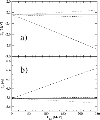
Figure 1: The deuteron binding energy $E_{d}$ and the D-state probability $P_{D}$. The values for the deuteron at rest are given by the solid horizontal lines. At different incoming nucleon lab. energies, related to the relative momentum $q_{0}$ in Eq. (6), the approximations given in Eqs.(67), (68), and (66) provide results which are shown as the dashed-, dotted-, and dashed-dotted lines, respectively. The calculations have been done with the AV18 potential.

IV Results

The solution of the 3N relativised Faddeev equation including Wigner spin rotations increase the computer time drastically. This is caused by the calculation of the permutation matrix elements for the high partial waves. Therefore to study the effects of the Wigner spin rotations on the elastic scattering observables we restricted ourselves to the $j<2$ partial wave states. We checked that to get converged results for the permutation matrix elements one has to take into account the expansion coefficients $a^{\mu_{2}\mu_{3}\mu_{2}^{\prime}\mu_{3}^{\prime}m_{1}m_{2}}_{LML^{\prime}M^{\prime}}(q,q^{\prime})$ of Eq.(104) with L,L’ up to L,L’$\leq 2$. Those coefficients were obtained by numerical integrations over the directions $\hat{q}$ and $\hat{q}^{\prime}$ with 23 gaussian points for the polar and azimuthal angles. We found that the changes of the cross sections due to Wigner spin rotations are small and stay under $1\%$. For spin observables these changes are slightly larger but they do not exceed $5\%$ with the exception of angular regions around zero crossings and small values of the observables. Thus when performing the fully converged calculations with $j\leq 5$ and $J\leq 25/2$ we neglected the Wigner spin rotations completely. This might be different for breakup observables, which deserves another investigation.

In Fig.2 we show our results for the nd elastic scattering cross sections at four energies together with experimental pd data. In addition to the nonrelativistic prediction, based on the solution of the 3N Faddeev equation with the nonrelativistic form of the free propagator $G_{0}$ and partial wave states constructed with standard Jacobi momenta, also our relativistic results using the approximations according to the Eqs.(67), (68), and (66) for the boosted potential matrix elements are presented. Thereby the other relativistic features in Eq. (36) have been kept. It is only the total neglection of the boost effect in $V({\vec{q}}\,)$ which leads to a clearly visible deviation from the nonrelativistic results. Taking the boost effect into account according to the approximations (41) and (39) reduces the effect drastically and only at the largest angles deviations from the nonrelativistic results are discernible. This is better seen in Fig. 3, where the quantity

$$\Delta\equiv{{({d\sigma\over{d\Omega}})^{rel}-({d\sigma\over{d\Omega}})^{nrel}}\over{({d\sigma\over{d\Omega}})^{nrel}}}$$ (69)

expressed in percentage is shown for the three approximations.

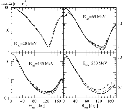
Figure 2: The differential cross sections for $Nd$ elastic scattering at various energies. The solid line is the result of the nonrelativistic Faddeev calculation with the AV18 potential. The relativistic predictions based on the approximations (67), (68), and (66) for the boosted potential keeping all other relativistic features unchanged are shown by the dashed, dotted, and dashed-dotted lines. The pd data at $28$, $65$, $135$ and $250$ MeV are from ref. hat84 , shi95 , sek02 , and hat02 , respectively.

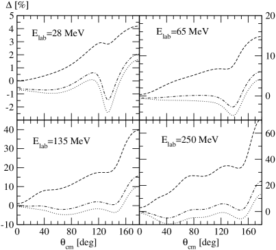
Figure 3: The relative deviation $\Delta$ from Eq. (69) for the three different relativistic approximations to the boosted potential $V({\vec{q}}\,)$. For the description of the lines see Fig.2.

Thus significant effects of relativity occur at higher energies and they are restricted to the backward angle region ($\theta_{c.m}\geq 160^{\circ}$). They increase the nonrelativistic cross sections by up to $2\%$, $6\%$, $5-15\%$, and $10-23\%$, for 28, 65, 135, and 250 MeV, respectively. For $\theta_{c.m}<160^{\circ}$ the effects of relativity are much smaller. At 250 MeV where they are largest, they increase the nonrelativistic cross section by no more than $\approx 5\%$ in the minimum around $\theta_{c.m}=130^{\circ}$. At forward angles the largest effects are at $\theta_{c.m}\approx 40^{\circ}$ where relativity reduces the nonrelativistic cross section by up to $\approx 5\%$.

In ref. wit99 the nd total cross section has been investigated in a nonrelativistic scheme. Beyond that a very first step into relativity has been done using the optical theorem. In our notation it reads

$$\sigma_{tot}=-{2\over{|\vec{j}|}}Im\,\sum\limits_{\mu_{n},\mu_{d}}<\phi~{}\mu_{n},\mu_{d}|U|\phi~{}\mu_{n},\mu_{d}>.$$ (70)

Now we can investigate the changes in both ingredients on the right hand side due to relativity, whereas in wit99 only the kinematical flux quantity $|{\vec{j}}|$ has been considered. The ratio of the relativistic to the nonrelativistic flux is given as

$${|\vec{j}|^{nrel}\over{|\vec{j}|^{rel}}}={E_{n}E_{d}\over{q_{0}^{rel}(E_{n}+E_{d})}}/{m_{d}m_{n}\over{q_{0}^{nrel}(m_{d}+m_{n})}},$$ (71)

where $E_{n}$ ($E_{d}$) is the neutron (deuteron) energy in the c.m. system and $q_{0}^{rel,nrel}$ the relativistic or nonrelativistic relative momentum in the c.m. system. In wit99 only that ratio was considered which led to an increase in the total cross section by 3 (7) % at 100 (250 ) MeV. Now allowing also for a change of the nuclear matrix element $<\phi|U|\phi>$ (using the approximate boosted potential given in Eq. (39)) the total cross section (not shown) is slightly smaller than the nonrelativistic one. In other words, the changes in $<\phi|U|\phi>$ outweigh the kinematical effect, which by itself increases the total cross section.

Now we come back to the elastic cross section which for the sake of completeness and clarity is shown. In our notation it has the form

$$\frac{(d\sigma)^{el,rel}}{d{\hat{q}}^{\,\prime}}=(2\pi)^{4}\left({E_{n}E_{d}\over{E_{n}+E_{d}}}\right)^{2}\,\frac{1}{6}\,\sum\limits_{\mu_{n}^{\prime},\mu_{d}^{\prime},\mu_{n},\mu_{d}}\,|<\phi^{\prime}~{}\mu_{n}^{\prime},\mu_{d}^{\prime}|U|\phi~{}\mu_{n},\mu_{d}>|^{2}.$$ (72)

The kinematical factor in the bracket reduces to $\frac{2m}{3}$ in the nonrelativistic case. Again we can regard the ratio of the relativistic and nonrelativistic differential cross sections. They are of different type compared to the ratio of the total cross sections. Both ingredients, the kinematical factor and the nuclear matrix element enter now squared. It turned out as we have seen in Figs. 2 and 3 that also in this case the dynamical effects caused by the decrease of the nuclear matrix element compensates the increase of the kinematical factor for most angles. Only at very backward angles a slight increase remains.

Finally in Figs.4-5 we compare relativistic and nonrelativistic predictions for the deuteron vector analyzing power $iT_{11}$. Again the three approximations to the boosted potential $V({\vec{q}}\,)$ are shown. It turns out that the relativistic effects are relatively small and they stay below $\approx 5\%$ in the angular regions outside of zero crossings. Other spin observables in elastic scattering behave similarly and are not shown.

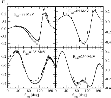
Figure 4: The deuteron vector analyzing power $iT_{11}$ in $Nd$ elastic scattering. For description of lines see Fig.2. The pd data at $28$, $65$, $135$ and $250$ MeV are from ref. hat84 , wit93 , sek02 , and cad01 , respectively. The pd data from cad01 were taken at $190$ MeV.

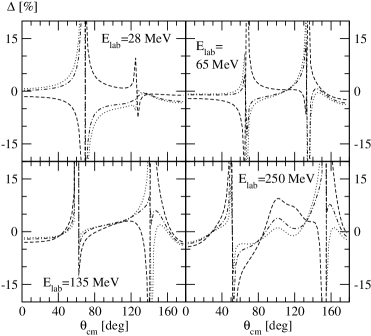
Figure 5: The same as in Fig.3 but for the deuteron vector analyzing power $iT_{11}$.

V Summary and outlook

We numerically solved the 3N Faddeev equation for nd scattering including relativistic features at the neutron lab energies $E_{n}^{lab}=28$, $65$, $135$ and $250$ MeV. The relativistic features are the relativistic form of the free propagator and the change of the NN potential caused by the boost of the 2N subsystem. In addition these boosts also induce Wigner spin rotations. For the momentum space basis we used the relative momentum of two free nucleons in their c.m. system together with their total momentum which in the 3N c.m. system is the negative momentum of the spectator nucleon. Such a choice of momenta is adequate for relativistic kinematics and allows to generalize the nonrelativistic approach used to solve the nonrelativistic 3N Faddeev equation to the relativistic case in a more or less straightforward manner. That relative momentum in the two-nucleon subsystem is a generalisation of the standard nonrelativistic Jacobi momentum $\vec{p}$. The inclusion of the nucleon spins leads automatically to Wigner spin rotations in the context of boosting the 2N c.m. subsystems. The momentum partial wave basis, a generalisation of the nonrelativistic one, is, however, now more complex. As dynamical input we took the nonrelativistic NN potential AV18 and generated in the 2N c.m. system an exactly on-shell equivalent relativistic interaction $v$ using an analytical scale transformation of momenta. We checked that in our energy range the boost effects for this potential could be sufficiently well incorporated by restricting the exact expression to the leading order terms in a $q/\omega$ and $v/\omega$ expansion.

We found that in the studied energy range the effects of Wigner spin rotations are practically negligible for the cross section and analyzing powers. Relativistic effects for the cross section appear at higher energies and they are restricted only to the very backward angles where relativity increases the nonrelativistic cross section. At other angles the effects are small. In spite of the fact that the relativistic phase-space factor increases with energy faster than the nonrelativistic one, the relativistic nuclear matrix element outweighs this increase and leads for the cross section in a wide angular range to a relatively small relativistic effect. Also for spin observables (analyzing powers, spin correlation coefficients and spin transfer coefficients, not shown) no drastic changes due to relativity have been found.

The comparison of our nonrelativistic theory with existing cross section data exhibits at the higher energies clear discrepancies. According to our presented results effects due to relativity are significant only in the region of very backward angles where they increase the cross section. They are relatively small in the region of the cross section minimum around $\theta_{cm}\approx 130^{\circ}$, where the discrepancies between the theory based on pairwise forces only and data are largest. At lower energies (up to about $\approx 135$ MeV) this discrepancy can be removed when current three-nucleon forces (3NFs), mostly of $2\pi$-exchange character TM ; uIX , are included in the nuclear Hamiltonian. At the higher energies, however, a significant part of the discrepancy remains and increases further with increasing energy. This indicates that additional 3N forces should be added to the $2\pi$-exchange type forces. Natural candidates in the traditional meson-exchange picture are exchanges like $\pi-\rho$ and $\rho-\rho$. This has to be expected since in $\chi$PT epel2002 in the order in which nonvanishing 3NF’s appear the first time there are three topologies of forces, the $2\pi$-exchange, a one-pion exchange between one nucleon and a two-nucleon contact interaction and a pure 3N contact interaction. They are of the same order and have to be kept together. Therefore it appears very worthwhile to persue a strategy adding in the traditional meson exchange picture further 3N forces. Our results here showing that relativistic effects based on relativistic kinematics and boost effects of the NN force are small support the usefulness of high energy elastic Nd scattering to study 3N force properties.

Appendix A The special boost matrix $\beta(k)$

The special Lorentz transformation $\beta(k)=\beta(~{}(\omega_{m}(\vec{k}),\vec{k})~{})$ is defined by $\beta(k)(m,\vec{0})=k$. It has the following matrix elements:

$$\beta_{ij} = \delta_{ij}+{{k_{i}\,k_{j}}\over{m(m+\omega_{m}(\vec{k}))}}~{}~{}~{}~{}(i,j=1,2,3)$$ (73)

$$\beta_{\mu 0} = \beta_{0\mu}={k_{\mu}\over{m}}~{}~{}~{}~{}~{}~{}~{}~{}~{}~{}~{}~{}~{}~{}~{}(\mu=0,1,2,3).$$ (74)

Appendix B The matrices of Wigner rotation

By straightforward calculation, the $3\times 3$ matrix $M$ related to the first equation in Eq. (32) is presented. The four-momentum $P$ is such that

$$\beta(P)~{}(\omega_{m}(\vec{k}),\vec{k})~{})=(\omega_{m}(\vec{p}_{2}),\vec{p}_{2})$$ (75)

$$\beta(P)~{}(\omega_{m}(\vec{k}),-\vec{k})~{})=(\omega_{m}(\vec{p}_{3}),\vec{p}_{3}).$$ (76)

We obtain ($i,j=1,2,3$)

$$M_{ij}=\delta_{ij}\ +\ f_{1}\,k_{i}\,k_{j}\ +\ f_{2}\,P_{i}\,k_{j}\ +\ f_{3}\,k_{i}\,P_{j}\ +\ f_{4}\,P_{i}\,P_{j},$$ (77)

where the four scalar functions $f_{1}$, $f_{2}$, $f_{3}$ and $f_{4}$ depend on the momenta ${\vec{k}}$ and ${\vec{P}}$:

$$f_{1}=\frac{-{E_{0}}+{M_{0}}}{\left(m+\frac{{M_{0}}}{2}\right)\,\left({{\vec{k}}\cdot{\vec{P}}}+\frac{{E_{0}}\,{M_{0}}}{2}+m\,{M_{0}}\right)}$$ (78)

$$f_{2}=\frac{2\,\left(4\,{{\vec{k}}\cdot{\vec{P}}}+\left({E_{0}}+{M_{0}}\right)\,\left(2\,m+{M_{0}}\right)\right)}{\left({E_{0}}+{M_{0}}\right)\,\left(2\,m+{M_{0}}\right)\,\left(2\,{{\vec{k}}\cdot{\vec{P}}}+\left({E_{0}}+2\,m\right)\,{M_{0}}\right)}$$ (79)

$$f_{3}=\frac{-2}{2\,{{\vec{k}}\cdot{\vec{P}}}+\left({E_{0}}+2\,m\right)\,{M_{0}}}$$ (80)

$$f_{4}=\frac{2\,m-{M_{0}}}{\left({E_{0}}+{M_{0}}\right)\,\left(2\,{{\vec{k}}\cdot{\vec{P}}}+\left({E_{0}}+2\,m\right)\,{M_{0}}\right)}$$ (81)

The quantities $M_{0}$ and $E_{0}$ are

$$M_{0}=2\sqrt{m^{2}+{\vec{k}}^{\ 2}}$$ (82)

and

$$E_{0}=\sqrt{M_{0}^{2}+{\vec{P}}^{\ 2}}.$$ (83)

The matrix $M$ related to the second equation in Eq. (32) results by replacing ${\vec{k}}$ by $-{\vec{k}}$. Clearly for ${\vec{P}}=0$ there is no rotation. If one expands $M_{ij}$ in terms of the components $P_{i}$ up to second order, a straightforward calculation leads to

$$\beta=\sqrt{\frac{4\,k_{3}^{2}}{M_{0}^{2}(2m+M_{0})^{2}}\,{\vec{P}}^{\,2}\ -\ \frac{8\,k_{3}P_{3}\,{\vec{k}}\cdot{\vec{P}}}{M_{0}^{2}(2m+M_{0})}\ +\ \frac{M_{0}-2m}{M_{0}^{2}(2m+M_{0})}\,P_{3}^{2}}\ +\ {\cal O}({\vec{P}}^{\,2})$$ (84)

This is useful numerically in the determination of the Euler angles $\alpha$, $\beta$ and $\gamma$. For $\beta=0$ only the combination ($\alpha+\gamma$) occurs and one can put for instance $\alpha=0$.

Appendix C Permutation operator

Using Eq. (30) twice for the bra state ${}_{1}<kq\alpha|$ and the ket state $|k^{\prime}q^{\prime}\alpha^{\prime}>_{2}$ one gets for the matrix element of the permutation operator in our partial wave basis:

$${}_{1}<k~{}q~{}\alpha|~{}P~{}|k^{\prime}~{}q^{\prime}~{}\alpha^{\prime}>_{1}=2~{}_{1}<k~{}q~{}\alpha~{}|~{}k^{\prime}~{}q^{\prime}~{}\alpha^{\prime}>_{2}=$$ (85)

$$2~{}\sum_{m_{1}m_{2}m_{3}}\sum_{\mu_{2}\mu_{3}\mu_{s}}\sum_{\mu_{l}\mu_{\lambda}\mu_{I}\mu}\sum_{\mu_{2}^{\prime}\mu_{3}^{\prime}\mu_{s^{\prime}}}\sum_{\mu_{l^{\prime}}\mu_{\lambda^{\prime}}\mu_{I^{\prime}}\mu^{\prime}}~{}$$ (86)

$$(\lambda\mu_{\lambda}{1\over{2}}m_{1}|I\mu_{I})~{}(j\mu I\mu_{I}|JM)~{}({1\over{2}}\mu_{2}{1\over{2}}\mu_{3}|s\mu_{s})~{}(l\mu_{l}s\mu_{s}|j\mu)$$ (87)

$$(\lambda^{\prime}\mu_{\lambda^{\prime}}{1\over{2}}m_{2}|I^{\prime}\mu_{I^{\prime}})~{}(j^{\prime}\mu^{\prime}I^{\prime}\mu_{I^{\prime}}|JM)~{}({1\over{2}}\mu_{2}^{\prime}{1\over{2}}\mu_{3}^{\prime}|s^{\prime}\mu_{s^{\prime}})~{}(l^{\prime}\mu_{l^{\prime}}s^{\prime}\mu_{s^{\prime}}|j^{\prime}\mu^{\prime})$$ (88)

$$\int d\hat{q}~{}d\hat{q}^{\prime}~{}{1\over{N(\vec{q}~{}^{\prime},-\vec{q}-\vec{q}~{}^{\prime})}}~{}{1\over{N(-\vec{q}-\vec{q}~{}^{\prime},\vec{q}~{})}}$$ (89)

$${\delta(~{}k-|\vec{k}(~{}\vec{q}~{}^{\prime},-\vec{q}-\vec{q}~{}^{\prime}~{})|~{})\over{k^{2}}}~{}{\delta(~{}k^{\prime}-|\vec{k}(~{}-\vec{q}-\vec{q}~{}^{\prime},\vec{q}~{})|~{})\over{{k^{\prime}}^{2}}}~{}$$ (90)

$$Y^{\lambda~{}*}_{\mu_{\lambda}}(\hat{q})~{}Y^{l~{}*}_{\mu_{l}}(\hat{k}(~{}\vec{q}~{}^{\prime},-\vec{q}-\vec{q}~{}^{\prime})~{})~{}Y^{\lambda^{\prime}}_{\mu_{\lambda^{\prime}}}(\hat{q}~{}^{\prime})~{}Y^{l^{\prime}}_{\mu_{l^{\prime}}}(\hat{k}(~{}-\vec{q}-\vec{q}~{}^{\prime},\vec{q}~{})~{})~{}$$ (91)

$$D^{{1\over{2}}~{}*}_{m_{2}\mu_{2}}(R(\beta(P(~{}\vec{q}~{}^{\prime},-\vec{q}-\vec{q}~{}^{\prime}~{})),\vec{k}(~{}\vec{q}~{}^{\prime},-\vec{q}-\vec{q}~{}^{\prime})~{}))~{}$$ (92)

$$D^{{1\over{2}}~{}*}_{m_{3}\mu_{3}}(R(\beta(P(~{}\vec{q}~{}^{\prime},-\vec{q}-\vec{q}~{}^{\prime}~{})),-\vec{k}(~{}\vec{q}~{}^{\prime},-\vec{q}-\vec{q}~{}^{\prime})~{}))~{}$$ (93)

$$D^{{1\over{2}}}_{m_{3}\mu_{2}^{\prime}}(R(\beta(P(~{}-\vec{q}-\vec{q}~{}^{\prime},\vec{q}~{})),\vec{k}(~{}-\vec{q}-\vec{q}~{}^{\prime},\vec{q}~{})~{}))~{}$$ (94)

$$D^{{1\over{2}}}_{m_{1}\mu_{3}^{\prime}}(R(\beta(P(~{}-\vec{q}-\vec{q}~{}^{\prime},\vec{q}~{})),-\vec{k}(~{}-\vec{q}-\vec{q}~{}^{\prime},\vec{q}~{})~{}))~{}$$ (95)

$${}_{1}<(~{}(t{1\over{2}})T~{}|~{}(t^{\prime}{1\over{2}})T~{}>_{2},$$ (96)

with

$$\vec{k}(~{}\vec{q}~{}^{\prime},-\vec{q}-\vec{q}~{}^{\prime})~{}\equiv~{}\vec{q}~{}^{\prime}+{1\over{2}}\vec{q}(1+y_{1}(q,q^{\prime},x))~{}$$ (97)

$$\vec{k}(~{}-\vec{q}-\vec{q}~{}^{\prime},\vec{q}~{})~{}\equiv~{}-\vec{q}-{1\over{2}}\vec{q}~{}^{\prime}(1+y_{2}(q,q^{\prime},x)).$$ (98)

In Eq.(98) occur

$$y_{1}(q,q^{\prime},x)=\frac{E_{{\vec{q}}^{\,\prime}}\,-\,E_{{\vec{q}}+{\vec{q}}^{\,\prime}}}{E_{{\vec{q}}^{\,\prime}}\,+\,E_{{\vec{q}}+{\vec{q}}^{\,\prime}}\ +\ \sqrt{(E_{{\vec{q}}^{\,\prime}}\,+\,E_{{\vec{q}}+{\vec{q}}^{\,\prime}})^{2}-{\vec{q}}^{\ 2}}}$$ (99)

with $x=\hat{q}\cdot\hat{q}^{\prime}$, $y_{2}(q,q^{\prime},x)=y_{1}(q^{\prime},q,x)$ and $E_{{\vec{q}}}\equiv\omega_{m}({\vec{q}~{}})$.

Expanding the product of the four D-matrices in Eq.(96) into spherical harmonics

$$\sum_{m_{3}}~{} D^{{1\over{2}}~{}*}_{m_{2}\mu_{2}}(R(\beta(P(~{}\vec{q}~{}^{\prime},-\vec{q}-\vec{q}~{}^{\prime}~{})),\vec{k}(~{}\vec{q}~{}^{\prime},-\vec{q}-\vec{q}~{}^{\prime})~{}))~{}$$ (100)

$$D^{{1\over{2}}~{}*}_{m_{3}\mu_{3}}(R(\beta(P(~{}\vec{q}~{}^{\prime},-\vec{q}-\vec{q}~{}^{\prime}~{})),-\vec{k}(~{}\vec{q}~{}^{\prime},-\vec{q}-\vec{q}~{}^{\prime})~{}))~{}$$ (101)

$$D^{{1\over{2}}}_{m_{3}\mu_{2}^{\prime}}(R(\beta(P(~{}-\vec{q}-\vec{q}~{}^{\prime},\vec{q}~{})),\vec{k}(~{}-\vec{q}-\vec{q}~{}^{\prime},\vec{q}~{})~{}))~{}$$ (102)

$$D^{{1\over{2}}}_{m_{1}\mu_{3}^{\prime}}(R(\beta(P(~{}-\vec{q}-\vec{q}~{}^{\prime},\vec{q}~{})),-\vec{k}(~{}-\vec{q}-\vec{q}~{}^{\prime},\vec{q}~{})~{}))~{}$$ (103)

$$=\sum_{LML^{\prime}M^{\prime}}a^{\mu_{2}\mu_{3}\mu_{2}^{\prime}\mu_{3}^{\prime}m_{1}m_{2}}_{LML^{\prime}M^{\prime}}(q,q^{\prime})~{}Y^{*}_{LM}(\hat{q})~{}Y_{L^{\prime}M^{\prime}}(\hat{q}~{}^{\prime})~{},$$ (104)

and performing the integrations over $\hat{q}$ and $\hat{q}^{\prime}$ in Eq.(96) leads to the following expression for the matrix element of the permutation operator P:

$${}_{1}<k~{}q~{}\alpha|~{}P~{}|k^{\prime}~{}q^{\prime}~{}\alpha^{\prime}>_{1} = \int_{-1}^{1}dx{{\delta(k-\pi_{1})}\over{k^{l+2}}}~{}{{\delta(k^{\prime}-\pi_{2})}\over{k^{\prime l^{\prime}+2}}}~{}$$ (105)

$${1\over{N_{1}(q,q^{\prime},x)}}~{}{1\over{N_{2}(q,q^{\prime},x)}}~{}G_{\alpha\alpha^{\prime}}(q,q^{\prime},x),$$ (106)

with

$$G_{\alpha\alpha^{\prime}}(q,q^{\prime},x) = \sum_{k}P_{k}(x)~{}\sum_{l_{1}+l_{2}=l}\sum_{l_{1}^{\prime}+l_{2}^{\prime}=l^{\prime}}q^{l_{2}+l_{2}^{\prime}}q~{}^{\prime l_{1}+l_{1}^{\prime}}(1+y_{1})^{l_{2}}(1+y_{2})^{l_{1}^{\prime}}g_{\alpha\alpha^{\prime}}^{kl_{1}l_{2}l_{1}^{\prime}l_{2}^{\prime}}(q,q^{\prime})$$ (107)

and

$$\pi_{1} = \sqrt{q^{\prime 2}+{1\over{4}}q^{2}(1+y_{1})^{2}+qq^{\prime}x(1+y_{1})}$$ (108)

$$\pi_{2} = \sqrt{q^{2}+{1\over{4}}q^{\prime 2}(1+y_{2})^{2}+qq^{\prime}x(1+y_{2})}$$ (109)

$$N_{1}(q,q^{\prime},x) \equiv N(\vec{q}~{}^{\prime},-\vec{q}-\vec{q}~{}^{\prime})$$ (110)

$$N_{2}(q,q^{\prime},x) \equiv N(-\vec{q}-\vec{q}~{}^{\prime},\vec{q}~{}).$$ (111)

The geometrical coefficients $g_{\alpha\alpha^{\prime}}^{kl_{1}l_{2}l_{1}^{\prime}l_{2}^{\prime}}(q,q^{\prime})$ are given by

$$g_{\alpha\alpha^{\prime}}^{kl_{1}l_{2}l_{1}^{\prime}l_{2}^{\prime}}(q,q^{\prime}) = \sum_{\mu_{2}\mu_{3}\mu_{2}^{\prime}\mu_{3}^{\prime}}\sum_{LML^{\prime}M^{\prime}}\sum_{m_{1}m_{2}}a^{\mu_{2}\mu_{3}\mu_{2}^{\prime}\mu_{3}^{\prime}m_{1}m_{2}}_{LML^{\prime}M^{\prime}}(q,q^{\prime})~{}A^{\mu_{2}\mu_{3}\mu_{2}^{\prime}\mu_{3}^{\prime}m_{1}m_{2}}_{LML^{\prime}M^{\prime}}(J^{\pi}\alpha\alpha^{\prime}kl_{1}l_{2}l_{1}^{\prime}l_{2}^{\prime}),$$ (112)

with

$$A^{\mu_{2}\mu_{3}\mu_{2}^{\prime}\mu_{3}^{\prime}m_{1}m_{2}}_{LML^{\prime}M^{\prime}} ( J^{\pi}\alpha\alpha^{\prime}kl_{1}l_{2}l_{1}^{\prime}l_{2}^{\prime})={1\over{4\pi}}(-1)^{t^{\prime}}\delta_{TT^{\prime}}\delta_{M_{T}M_{T^{\prime}}}\sqrt{\hat{t}\hat{t}^{\prime}}\left\{\matrix{1/2&1/2&t\cr 1/2&T&t^{\prime}\cr}\right\}$$ (113)

$$(-1)^{k}\hat{k}({1\over{2}})^{l_{2}}({1\over{2}})^{l_{1}^{\prime}}(-1)^{l^{\prime}}\sqrt{\hat{\lambda}\hat{\lambda}^{\prime}}\sqrt{{{(\hat{l}^{\prime})!}\over{(2l_{1}^{\prime})!(2l_{2}^{\prime})!}}}\sqrt{{{(\hat{l})!}\over{(\hat{l}_{1})!(\hat{l}_{2})!}}}{{\sqrt{\hat{L}\hat{L}^{\prime}}}\over{\sqrt{\hat{l}_{2}\hat{l}_{1}}}}$$ (114)

$$({1\over{2}}\mu_{2}{1\over{2}}\mu_{3}|s\mu_{2}+\mu_{3})~{}({1\over{2}}\mu_{2}^{\prime}{1\over{2}}\mu_{3}^{\prime}|s^{\prime}\mu_{2}^{\prime}+\mu_{3}^{\prime})~{}\sum_{c_{1}}(L0\lambda 0|c_{1}0)~{}\sum_{c_{1}^{\prime}}(L^{\prime}0\lambda^{\prime}0|c_{1}^{\prime}0)~{}$$ (115)

$$\sum_{\mu_{\lambda}}(LM\lambda\mu_{\lambda}|c_{1}M+\mu_{\lambda})~{}(-1)^{M+\mu_{\lambda}}(\lambda\mu_{\lambda}{1\over{2}}m_{1}|I\mu_{\lambda}+m_{1})~{}$$ (116)

$$\sum_{\mu}(j\mu I\mu_{\lambda}+m_{1}|J\mu+\mu_{\lambda}+m_{1})~{}(l\mu-\mu_{2}-\mu_{3}s\mu_{2}+\mu_{3}|j\mu)~{}$$ (117)

$$\sum_{\mu^{\prime}}(j^{\prime}\mu^{\prime}I^{\prime}\mu+\mu_{\lambda}+m_{1}-\mu^{\prime}|J\mu+\mu_{\lambda}+m_{1})~{}(l^{\prime}\mu^{\prime}-\mu_{2}^{\prime}-\mu_{3}^{\prime}s^{\prime}\mu_{2}^{\prime}+\mu_{3}^{\prime}|j^{\prime}\mu^{\prime})~{}$$ (118)

$$(\lambda^{\prime}\mu+\mu_{\lambda}+m_{1}-\mu^{\prime}-m_{2}{1\over{2}}m_{2}|I^{\prime}\mu+\mu_{\lambda}+m_{1}-\mu^{\prime})~{}$$ (119)

$$(L^{\prime}M^{\prime}\lambda^{\prime}\mu+\mu_{\lambda}+m_{1}-\mu^{\prime}-m_{2}|c_{1}^{\prime}\mu+\mu_{\lambda}+m_{1}-\mu^{\prime}-m_{2}+M^{\prime})~{}$$ (120)

$$\sum_{f_{1}}(k0l_{1}^{\prime}0|f_{1}0)\sqrt{\hat{f}_{1}}(c_{1}^{\prime}0f_{1}0|l_{1}0)~{}\sum_{f_{2}}(k0l_{2}^{\prime}0|f_{2}0)\sqrt{\hat{f}_{2}}(c_{1}0f_{2}0|l_{2}0)~{}\left\{\matrix{f_{2}&f_{1}&l^{\prime}\cr l_{1}^{\prime}&l_{2}^{\prime}&k\cr}\right\}~{}$$ (121)

$$\sum_{m_{l_{1}}}(l_{1}m_{l_{1}}l_{2}\mu-\mu_{2}-\mu_{3}-m_{l_{1}}|l\mu-\mu_{2}-\mu_{3})~{}$$ (122)

$$(c_{1}-M-\mu_{\lambda}f_{2}\mu-\mu_{2}-\mu_{3}-m_{l_{1}}+M+\mu_{\lambda}|l_{2}\mu-\mu_{2}-\mu_{3}-m_{l_{1}})~{}$$ (123)

$$(f_{1}m_{f_{1}}f_{2}m_{f_{2}}|l^{\prime}\mu^{\prime}-\mu_{2}^{\prime}-\mu_{3}^{\prime})~{}$$ (124)

$$(c_{1}^{\prime}\mu+\mu_{\lambda}+m_{1}-\mu^{\prime}-m_{2}+M^{\prime}f_{1}m_{f_{1}}|l_{1}m_{l_{1}}).$$ (125)

We used our standard notation ${\hat{l}}\equiv 2\,l+1$. The coefficients $A^{\mu_{2}\mu_{3}\mu_{2}^{\prime}\mu_{3}^{\prime}m_{1}m_{2}}_{LML^{\prime}M^{\prime}}(J^{\pi}\alpha\alpha^{\prime}kl_{1}l_{2}l_{1}^{\prime}l_{2}^{\prime})$ are real and obey the following symmetry property

$$A^{-\mu_{2}-\mu_{3}-\mu_{2}^{\prime}-\mu_{3}^{\prime}-m_{1}-m_{2}}_{L-ML^{\prime}-M^{\prime}}(J^{\pi}\alpha\alpha^{\prime}kl_{1}l_{2}l_{1}^{\prime}l_{2}^{\prime})=A^{\mu_{2}\mu_{3}\mu_{2}^{\prime}\mu_{3}^{\prime}m_{1}m_{2}}_{LML^{\prime}M^{\prime}}(J^{\pi}\alpha\alpha^{\prime}kl_{1}l_{2}l_{1}^{\prime}l_{2}^{\prime}).$$ (126)

The proof involves in addition to the definition (125) the properties $l_{1}+l_{2}=l$, $l_{1}^{\prime}+l_{2}^{\prime}=l^{\prime}$ and the parity conservation: $(-1)^{l+\lambda}=(-1)^{l^{\prime}+\lambda^{\prime}}$. The coefficients $a^{\mu_{2}\mu_{3}\mu_{2}^{\prime}\mu_{3}^{\prime}m_{1}m_{2}}_{LML^{\prime}M^{\prime}}(q,q^{\prime})$, defined in (104), are complex and obey

$$a^{*\mu_{2}\mu_{3}\mu_{2}^{\prime}\mu_{3}^{\prime}m_{1}m_{2}}_{LML^{\prime}M^{\prime}}(q,q^{\prime})=(-1)^{M+M^{\prime}+m_{2}-\mu_{2}-\mu_{3}-\mu_{2}^{\prime}+m_{1}-\mu_{3}^{\prime}+1}~{}a^{-\mu_{2}-\mu_{3}-\mu_{2}^{\prime}-\mu_{3}^{\prime}-m_{1}-m_{2}}_{L-ML^{\prime}-M^{\prime}}(q,q^{\prime}).$$ (127)

To obtain (127) one uses the relation $D^{j\ *}_{mm^{\prime}}(\alpha,\beta,\gamma)=(-1)^{m-m^{\prime}}\,D^{j}_{-m-m^{\prime}}(\alpha,\beta,\gamma)$. The two last Clebsch-Gordan coefficients in Eq. (125) provide the condition that the phase factor in Eq. (127) is one. Thus the geometrical coefficients $g_{\alpha\alpha^{\prime}}^{kl_{1}l_{2}l_{1}^{\prime}l_{2}^{\prime}}(q,q^{\prime})$ are real.

References

• (1) R.B. Wiringa, V.G.J. Stoks, R. Schiavilla, Phys. Rev. C51, 38 (1995).
• (2) R. Machleidt, F. Sammarruca, and Y. Song, Phys. Rev. C53, R1483 (1996).
• (3) V.G.J. Stoks, R.A.M. Klomp, C.P.F. Terheggen, J.J. de Swart, Phys. Rev. C49, 2950 (1994).
• (4) J.L. Friar et al., Phys. Lett. B311, 4 (1993).
• (5) A. Nogga, D. Hüber, H. Kamada, and W. Glöckle, Phys. Lett. B409, 19 (1997).
• (6) H. Witała, W. Glöckle, D. Hüber, J. Golak, and H. Kamada, Phys. Rev. Lett. 81, 1183 (1998).
• (7) K. Sekiguchi et al., Phys. Rev. C65, 034003 (2002).
• (8) H. Witała et al., Phys. Rev. C63, 024007 (2001).
• (9) W.P. Abfalterer et al., Phys. Rev. Lett. 81, 57 (1998).
• (10) H. Witała et al., Phys. Rev. C59, 3035 (1999).
• (11) G. Rupp and J.A. Tjon, Phys. Rev. C45, 2133 (1992).
• (12) F. Sammarruca and R. Machleidt, Few-Body Syst. 24, 87 (1998).
• (13) A. Stadler, F. Gross, and M.Frank, Phys. Rev. C56, 2396 (1997); A. Stadler and F. Gross, Phys. Rev. Lett. 78, 26 (1997).
• (14) B. Bakamjian and L.H. Thomas, Phys. Rev. 92, 1300 (1952).
• (15) L.L. Foldy, Phys. Rev. 122, 275 (1961); R.A. Krajcik and L.L. Foldy, Phys. Rev. D10, 1777 (1974).
• (16) B.D. Keister, in Few-Body Problems in Physics, edite by Paul Schoessow, AIP Conf. Proc. No. 334, (AIP, Woodbury, NY, 1995), p.164.
• (17) B.D. Keister and W.N. Polyzou, Adv. Nucl. Phys. 20, 225 (1991).
• (18) H. Kamada, W. Glöckle, J. Golak, and Ch. Elster, Phys. Rev. C66, 044010 (2002).
• (19) W. Glöckle, T-S. H. Lee, and F. Coester, Phys. Rev. C33, 709 (1986).
• (20) H. Kamada, W. Glöckle, Phys. Rev. Lett. 80, 2547 (1998).
• (21) H.Witała, T.Cornelius and W.Glöckle, Few-Body Syst. 3, 123 (1988).
• (22) W. Glöckle, H.Witała, D.Hüber, H.Kamada, J.Golak, Phys.Rep. 274, 107 (1996).
• (23) F. Coester, Helv. Phys. Acta 38, 7 (1965).
• (24) W.Glöckle, The Quantum Mechanical Few-Body Problem, Springer-Verlag 1983.
• (25) S. Weinberg, The quantum theory of fields, vol. I, Cambridge University Press, 1995.
• (26) M.E. Rose, “Elementary theory of angular momentum”, Dover publications, Inc, New York, 1995.
• (27) H. Kamada, Few-Body Syst. Suppl.12, 433 (2000).
• (28) K. Hatanaka et al., Nucl. Phys. A 426, 77 (1984).
• (29) S. Shimizu et al., Phys. Rev. C52, 1193 (1995).
• (30) K. Hatanaka et al., Phys. Rev. C66, 044002 (2002).
• (31) H.Witała et al., Few-Body Syst. 15, 67 (1993).
• (32) R.V. Cadman et al., Phys. Rev. Lett. 86, 967 (2001).
• (33) S.A. Coon et al., Nucl. Phys. A317, 242 (1979); S.A. Coon and W. Glöckle, Phys. Rev. C23, 1790 (1981).
• (34) B.S. Pudliner et al., Phys. Rev. C56, 1720 (1997).
• (35) E. Epelbaum et al., Phys. Rev. C 66, 064001 (2002).