Collective Paths Connecting the Oblate and Prolate Shapes in ⁶⁸Se and ⁷²Kr Suggested by the Adiabatic Self-Consistent Collective Coordinate Method

Abstract

By means of the adiabatic self-consistent collective coordinate method and the pairing-plus-quadrupole interaction, we have obtained the self-consistent collective path connecting the oblate and prolate local minima in ⁶⁸Se and ⁷²Kr for the first time. The self-consistent collective path is found to run approximately along the valley connecting the oblate and prolate local minima in the collective potential energy landscape. This result of calculation clearly indicates the importance of triaxial deformation dynamics in oblate-prolate shape coexistence phenomena.

1 Introduction

Microscopic description of large amplitude collective motion in nuclei is a long-standing fundamental subject of nuclear structure physics [1, 2, 3, 4, 5]. In spite of the steady development in various theoretical concepts and mathematical formulations of them, application of the microscopic many-body theory to actual nuclear phenomena still remains as a challenging subject.^6)-33) Shape coexistence phenomena are typical examples of large amplitude collective motion in nuclei, and active investigations are currently going on both experimentally and theoretically.^34)-57) We are particularly interested in the recent discovery of coexisting two rotational bands in ⁶⁸Se and ⁷²Kr, which are associated with oblate and prolate intrinsic shapes[41, 42]. Clearly, these data strongly call for further development of the theory which is able to describe them and renew our concepts of nuclear structure. From the viewpoint of the microscopic mean-field theory, coexistence of different shapes implies that different solutions of the Hartree-Fock-Bogoliubov (HFB) equations (local minima in the deformation energy surface) appear in the same energy region and that the nucleus exhibits large amplitude collective motion connecting these different equilibrium points. The identities and mixings of these different shapes are determined by the dynamics of such collective motion.

On the basis of the time-dependent Hartree-Fock (TDHF) theory, the selfconsistent collective coordinate (SCC) method was proposed as a microscopic theory of such large amplitude collective motions [12]. It was extended to the case of time-dependent HFB (TDHFB) including the pairing correlations[23], and has been successfully applied to various kinds of anharmonic vibration and high-spin rotations [58, 59, 60, 61, 62, 63, 64, 65, 66, 67, 68, 69]. In order to apply this method to shape coexistence phenomena, however, we need to further develop the theory, since the known method of solving the basic equations of the SCC method, called $\eta$-expansion method[12], assumes a single local minima whereas several local minima of the potential energy surface compete in these phenomena. Some years ago, we proposed a new method of describing such large-amplitude collective motion, called the adiabatic self-consistent collective coordinate (ASCC) method[70]. This method provides a practical scheme of solving the basic equations of the SCC method[12] using an expansion in terms of the collective momentum. It does not assume a single local minimum, and therefore it is believed to be suitable for the description of shape coexistence phenomena. The ASCC method inherits the major achievement of the adiabatic TDHF (ATDHF) methods and, in addition, enables us to include pairing correlations self-consistently. In this method, the spurious number fluctuation modes are automatically decoupled from the physical modes within a selfconsistent framework of the TDHFB theory. This will be a great advantage when the method is applied to realistic nuclear problems. To examine the feasibility of the ASCC method, in Ref. kob03, we applied it to an exactly solvable model called the multi-$O(4)$ model[72, 73, 74, 75], which is a simplified version of the pairing-plus-quadrupole (P+Q) interaction model[76, 77, 78]. It was shown that this method yields a faithful description of tunneling motion through a barrier between prolate and oblate local minima in the collective potential[71].

In this paper, we report on our first application of the ASCC method to the P+Q interaction model. The major task here is to develop a practical procedure for solving the basic equations of the ASCC method in order to obtain the selfconsistent collective path. We investigate, as typical examples, the oblate-prolate shape coexistence phenomena in ⁶⁸Se and ⁷²Kr[41, 42], and find that the self-consistent collective paths run approximately along the valley connecting the oblate and prolate local minima in the collective potential energy landscape. To the best of our knowledge, this is the first time that, starting from the microscopic P+Q Hamiltonian, the collective paths have been fully self-consistently obtained for realistic situations, although a similar approach to the study of large amplitude collective motion was recently employed by Almehed and Walet[79, 80].

This paper is organized as follows: In §2, the basic equations of the ASCC method are recapitulated. In §3, we present a concrete formulation of the ASCC method for the case of the P+Q Hamiltonian. In §4, an algorithm to solve the basic equations of the ASCC method is discussed. In §5, we present results of numerical calculation for the oblate-prolate shape coexistence phenomena in ⁶⁸Se and ⁷²Kr. Concluding remarks are given in §6.

A preliminary version of this work was reported in this journal[81].

2 Basic equations of the ASCC method

In this section, we summarize the basic equations of the ASCC method[70]. The basic assumption of our approach is that large-amplitude collective motions can be described by a set of time-dependent HFB state vectors $\left|\phi(q,p,\varphi,N)\right\rangle$ parameterized by a single collective coordinate $q$, the collective momentum $p$ conjugate to $q$, the particle number $N$ and the gauge angle $\varphi$ conjugate to $N$. Then, the state vectors can be written in the following form:

$$\left|\phi(q,p,\varphi,N)\right\rangle=e^{-i\varphi\hat{N}}\left|\phi(q,p,N)\right\rangle=e^{-i\varphi\hat{N}}e^{ip{\hat{Q}(q)}}|\phi(q)\rangle.$$ (1)

Making an expansion with respect to $p$ and requiring that the time-dependent variational principle be fulfilled up to the second order in $p$, we obtain the following set of equations to determine $\left|\phi(q)\right\rangle$, the infinitesimal generator $\hat{Q}(q)$, and its canonical conjugate $\hat{P}(q)$:

HFB equation in the moving frame:

$$\delta\left\langle\phi(q)\right|\hat{H}_{M}(q)\left|\phi(q)\right\rangle=0,$$ (2)

where

$$\hat{H}_{M}(q)=\hat{H}-\lambda(q)\hat{N}-\frac{\partial V}{\partial q}\hat{Q}(q)$$ (3)

represents the Hamiltonian in the moving frame.

Local Harmonic equations in the moving frame:

$$\delta\left\langle\phi(q)\right|[\hat{H}_{M}(q),\hat{Q}(q)]-{1\over i}B(q)\hat{P}(q)\left|\phi(q)\right\rangle=0,$$ (4)

$$\delta\left\langle\phi(q)\right|[\hat{H}_{M}(q),{1\over i}\hat{P}(q)]-C(q)\hat{Q}(q)-{1\over 2B(q)}[[\hat{H}_{M}(q),(\hat{H}-\lambda(q)\hat{N})_{A}],\hat{Q}(q)]-{\partial\lambda\over\partial q}\hat{N}\left|\phi(q)\right\rangle=0,$$ (5)

where

$$B(q)=-\left\langle\phi(q)\right|[[\hat{H},\hat{Q}(q)],\hat{Q}(q)]\left|\phi(q)\right\rangle.$$ (6)

represents the inverse mass,

$$C(q)={\partial^{2}V\over\partial q^{2}}+{1\over 2B(q)}{\partial B\over\partial q}{\partial V\over\partial q}$$ (7)

the local stiffness, and $(\hat{H}-\lambda\hat{N})_{A}$ denotes the two-quasiparticle creation and annihilation parts of ($\hat{H}-\lambda\hat{N}$).

The infinitesimal generators, $\hat{Q}(q)$ and $\hat{P}(q)$, satisfy

Canonical variable condition:

$$\left\langle\phi(q)\right|[\hat{Q}(q),\hat{P}(q)]\left|\phi(q)\right\rangle=i.$$ (8)

Once $\left|\phi(q)\right\rangle$ and the infinitesimal generators are determined for every values of $q$, we obtain the collective Hamiltonian ${\cal H}(q,p)={1\over 2}B(q)p^{2}+V(q)$ with the collective potential $V(q)=\left\langle\phi(q)\right|\hat{H}\left|\phi(q)\right\rangle$.

In the above equations, no distinction is made between protons and neutrons for simplicity of notation. In the actual calculations described below, however, we shall explicitly treat both the neutron number $N$ and the proton number $Z$.

3 Application of the ASCC method to the P+Q model

3.1 The P+Q Hamiltonian and signature quantum number

Let us start with the well-known P+Q Hamiltonian[76, 77, 78],

$${\hat{H}}=\sum_{k}\epsilon_{k}c_{k}^{{\dagger}}c_{k}-\sum_{\tau}\frac{G_{\tau}}{2}\Big{(}A_{\tau}^{{\dagger}}A_{\tau}+A_{\tau}A_{\tau}^{{\dagger}}\Big{)}-\frac{\chi}{2}\sum_{K=-2}^{2}D_{2K}^{{\dagger}}D_{2K}.$$ (9)

$$A_{\tau}^{{\dagger}} = {\sum_{k\in\tau}}^{\prime}c_{k}^{{\dagger}}c_{\tilde{k}}^{{\dagger}},~{}~{}~{}A_{\tau}={\sum_{k\in\tau}}^{\prime}c_{\tilde{k}}c_{k},$$

$$D_{2K} = \sum_{\tau=n,p}\sum_{kl\in\tau}D_{2K}^{(\tau)}(kl)c_{k}^{\dagger}c_{l}$$ (10)

Here, $D_{2K}^{(\tau)}(kl)=\alpha_{\tau}^{2}\left\langle k\right|r^{2}Y_{2K}\left|l\right\rangle$;  $G_{\tau}$ and $\chi$ denote the pairing and quadrupole force strengths, respectively; $c_{k}^{{\dagger}}$ and $c_{k}$ are nucleon creation and annihilation operators in the single-particle state $k$, while $c_{\tilde{k}}^{{\dagger}}$ and $c_{\tilde{k}}$ denote those in the time reversed state of $k$. The index $\tau$ indicates protons ($\tau=p$) and neutrons($\tau=n$). Although we shall not explicitly mention below, it should be keep in mind that the single-particle index $k$ actually includes the index $\tau$. The notation ${\rm\Sigma}^{\prime}$ in the pair operators, $A_{\tau}^{{\dagger}}$ and $A_{\tau}$, indicates the sum over the pairs $(k,{\tilde{k}})$. The factors, $\alpha_{n}=(2Z/A)^{2/3}$ and $\alpha_{p}=(2N/A)^{2/3}$, attached to the quadrupole matrix elements guarantee equivalent root-mean-square radii for protons and neutrons. Following Baranger and Kumar[77], we take into account two major shells as a model space, and multiply a reduction factor $\zeta=(N_{L}+3/2)/(N_{L}+5/2)$ to the quadrupole matrix elements $D_{2K}^{(\tau)}(kl)$ of the upper harmonic-oscillator shell, $N_{L}$ being the total oscillator quanta of the lower shell. According to the conventional prescription of the P+Q interaction[76, 77, 78], we ignore the exchange (Fock) terms. Namely, we employ the Hartree-Bogoliubov (HB) approximation throughout this paper.

We introduce the notations,

$${\hat{F}}_{s}^{(\pm)} = \frac{1}{2}({\hat{F}}_{s}\pm{\hat{F}}_{s}^{{\dagger}}),$$

$${\hat{F}}_{s}^{(\pm)} = \{A_{n}^{(\pm)},A_{p}^{(\pm)},D_{20}^{(\pm)},D_{21}^{(\pm)},D_{22}^{(\pm)}\}~{}~{}~{}~{}~{}(s=1-5),$$ (11)

and write the P+Q Hamiltonian in the following form:

$${\hat{H}} = \sum_{k}\epsilon_{k}c_{k}^{{\dagger}}c_{k}-\sum_{s=1}^{5}\frac{\kappa_{s}}{2}{\hat{F}}_{s}^{(+)}{\hat{F}}_{s}^{(+)}+\sum_{s=1}^{5}\frac{\kappa_{s}}{2}{\hat{F}}_{s}^{(-)}{\hat{F}}_{s}^{(-)},$$ (12)

where $\kappa_{s}=\{2G_{n},2G_{p},\chi,2\chi,2\chi\}$ for $s=1-5$. Our Hamiltonian is invariant with respect to the rotation $\pi$ about the $x$ axis. The symmetry quantum number associated with it is called signature, $r=e^{-i\pi\alpha}$. To exploit the signature symmetry, it is convenient to use nucleon operators with definite signatures defined by

$$d_{k} \equiv \frac{1}{\sqrt{2}}(c_{k}+c_{\tilde{k}}),~{}~{}~{}~{}~{}r=-i~{}(\alpha=1/2),$$

$$d_{{\bar{k}}} \equiv \frac{1}{\sqrt{2}}(c_{\tilde{k}}-c_{k}),~{}~{}~{}~{}~{}r=+i~{}(\alpha=-1/2),$$ (13)

and their Hermite conjugates, $d_{k}^{{\dagger}}$ and $d_{{\bar{k}}}^{{\dagger}}$. The operators ${\hat{F}}_{s}^{(\pm)}$ are then classified according to the signature quantum numbers, $r=\pm 1$ ($\alpha=0,1$):

$$\{A_{n}^{(\pm)},A_{p}^{(\pm)},D_{20}^{(+)},D_{21}^{(-)},D_{22}^{(+)}\}~{}~{}~{}~{}~{}(r=+1),$$

$$\{D_{21}^{(+)},D_{22}^{(-)}\}~{}~{}~{}~{}~{}(r=-1).$$ (14)

Note that $D_{20}^{(-)}=0$. The HB local minima corresponding to the oblate and prolate equilibrium shapes possess positive signature, $r=+1(\alpha=0)$. Therefore, the operators, ${\hat{Q}}(q)$ and ${\hat{P}}(q)$, generating large amplitude collective motions associated with these shapes also possess positive signature. In other words, the negative signature degrees of freedom are exactly decoupled from the large amplitude collective motion of interest, so that we can ignore them. Also, it is readily confirmed that the $K=1$ components associated with the quadrupole operator ${\hat{D}}_{21}^{(-)}$ exactly decouple from the $K=0$ and 2 components in the local harmonic equations, (2.2) and (2.4). As is well known, they are associated with the collective rotational motions, and the large amplitude shape vibrational motions under consideration are exactly decoupled from them in the present framework. We note, however, that it is possible, by a rather straightforward extension, to formulate the ASCC method in a rotating frame of reference. By means of such an extension, we shall be able to take into account the coupling effects between the two kinds of large amplitude collective motion. It is certainly a very interesting subject to study how the properties of the large-amplitude shape vibrational motions change as a function of angular momentum, but it goes beyond the scope of this paper. We note, however, that some attempts toward this subject was recently made by Almehed and Walet[80].

Thus, only the components, $\{A_{n}^{(\pm)},A_{p}^{(\pm)},D_{20}^{(+)},D_{22}^{(+)}\}$, are pertinent to the shape coexistence dynamics of our interest. They all belong to the positive signature sector, and we can adopt a phase convention with which single-particle matrix elements of them are real. In the following, we assume that this is the case.

3.2 Quasiparticle-random-phase approximation (QRPA) at the HB local minima

As discussed in the introduction, shape coexistence phenomena imply the existence of several local minima in the deformation energy surface, which are solutions of the HB equations. Let us choose one of them and denote it as ${\left|\phi_{0}\right\rangle}$. The HB equation is written

$$\delta{\left\langle\phi_{0}\right|}{\hat{H}}-\sum_{\tau}\lambda_{\tau}{\hat{N}}_{\tau}{\left|\phi_{0}\right\rangle}=0,$$ (15)

where $\lambda_{\tau}$ denote chemical potentials for protons($\tau=p$) and neutrons($\tau=n$). The quasiparticle creation and annihilation operators, $a_{\mu}^{{\dagger}}$ and $a_{\mu}$, associated with the HB local minimum are defined by $a_{\mu}|\phi_{0}\rangle=0$. Similar equations hold for their signature partners $\bar{\mu}$. They are introduced through the Bogoliubov transformations:

$$\left(\begin{array}[]{c}a_{\mu}^{{\dagger}}\\ a_{\bar{\mu}}\end{array}\right)=\sum_{k}\left(\begin{array}[]{cc}U_{\mu k}&V_{\mu\bar{k}}\\ V_{\bar{\mu}k}&U_{\bar{\mu}\bar{k}}\end{array}\right)\left(\begin{array}[]{c}d_{k}^{{\dagger}}\\ d_{\bar{k}}\end{array}\right),$$ (16)

and their Hermite conjugate equations. (Here and hereafter, we do not mix protons and neutrons in these transformations.) In terms of two quasiparticle creation and annihilation operators,

$${\mbox{\boldmath$A$}_{\mu\bar{\nu}}^{{\dagger}}}\equiv a_{\mu}^{{\dagger}}a_{\bar{\nu}}^{{\dagger}},~{}~{}~{}{\mbox{\boldmath$A$}_{\mu\bar{\nu}}}\equiv a_{\bar{\nu}}a_{\mu},$$ (17)

the RPA normal coordinates and momenta describing small amplitude vibrations about the HB local minimum ${\left|\phi_{0}\right\rangle}$ are written

$${\hat{Q}}_{\rho} = \sum_{\mu\bar{\nu}}Q_{\mu\bar{\nu}}^{\rho}({\mbox{\boldmath$A$}_{\mu\bar{\nu}}^{{\dagger}}}+{\mbox{\boldmath$A$}_{\mu\bar{\nu}}}),$$ (18)

$${\hat{P}}_{\rho} = i\sum_{\mu\bar{\nu}}P_{\mu\bar{\nu}}^{\rho}({\mbox{\boldmath$A$}_{\mu\bar{\nu}}^{{\dagger}}}-{\mbox{\boldmath$A$}_{\mu\bar{\nu}}}),$$ (19)

where the sum is taken over the proton and neutron quasiparticle pairs $(\mu\bar{\nu})$, and $\rho$ labels the QRPA modes. The amplitudes, $Q_{\mu\nu}^{\rho}$ and $P_{\mu\nu}^{\rho}$, are determined by the QRPA equations of motion,

$$\delta\left\langle\phi_{0}\right|[\hat{H}-\sum_{\tau}\lambda_{\tau}\hat{N}_{\tau},~{}\hat{Q}_{\rho}]-{1\over i}B_{\rho}\hat{P}_{\rho}\left|\phi_{0}\right\rangle=0,$$ (20)

$$\delta\left\langle\phi_{0}\right|[\hat{H}-\sum_{\tau}\lambda_{\tau}\hat{N}_{\tau},~{}{1\over i}\hat{P}_{\rho}]-C_{\rho}\hat{Q}_{\rho}\left|\phi_{0}\right\rangle=0,$$ (21)

and the orthonormalization condition, $\left\langle\phi_{0}\right|[\hat{Q}_{\rho},\hat{P}_{\rho^{\prime}}]\left|\phi_{0}\right\rangle=i\delta_{\rho,\rho^{\prime}}$.

3.3 The HB equation and the quasiparticles in the moving frame

For the P+Q Hamiltonian, the HB equation (2) determining the state vector $|\phi(q)\rangle$ away from the local minimum reduces to

$$\delta\left\langle\phi(q)\right|\hat{h}_{M}(q)\left|\phi(q)\right\rangle=0,$$ (22)

where $\hat{h}_{M}(q)$ is the mean-field Hamiltonian in the moving frame,

$$\hat{h}_{M}(q) = \hat{h}(q)-\sum_{\tau}\lambda_{\tau}(q)\hat{N}_{\tau}-{\partial V\over\partial q}\hat{Q}(q),$$ (23)

$$\hat{h}(q) = \sum_{k}\epsilon_{k}(d_{k}^{{\dagger}}d_{k}+d_{\bar{k}}^{{\dagger}}d_{\bar{k}})-\sum_{s}\kappa_{s}\hat{F}^{(+)}_{s}\left\langle\phi(q)\right|\hat{F}^{(+)}_{s}\left|\phi(q)\right\rangle.$$ (24)

The state vector $|\phi(q)\rangle$ can be written as a unitary transform of $|\phi_{0}\rangle$:

$$\left|\phi(q)\right\rangle = e^{{\hat{\theta}}(q)}\left|\phi_{0}\right\rangle,$$

$${\hat{\theta}}(q) \equiv \sum_{\mu\bar{\nu}}\theta_{\mu\bar{\nu}}(q)\Big{(}\mbox{\boldmath$A$}_{\mu\bar{\nu}}^{{\dagger}}-\mbox{\boldmath$A$}_{\mu\bar{\nu}}\Big{)},$$ (25)

where the sum is taken over the proton and neutron quasiparticle pairs $(\mu\bar{\nu})$. The quasiparticle creation and annihilation operators, $a_{\mu}^{{\dagger}}(q)$ and $a_{\mu}(q)$, associated with the state $|\phi(q)\rangle$, which satisfy the condition, $a_{\mu}(q)|\phi(q)\rangle=0$, are written:

$$a_{\mu}^{{\dagger}}(q) \equiv e^{\hat{\theta}}(q)a_{\mu}^{{\dagger}}e^{-{\hat{\theta}}(q)}=\sum_{\nu}\Big{(}U_{\mu\nu}(q)a_{\nu}^{{\dagger}}+V_{\mu\bar{\nu}}(q)a_{\bar{\nu}}\Big{)},$$

$$a_{\bar{\mu}}(q) \equiv e^{\hat{\theta}}(q)a_{\bar{\mu}}e^{-{\hat{\theta}}(q)}=\sum_{\nu}\Big{(}V_{\bar{\mu}\nu}(q)a_{\nu}^{{\dagger}}+U_{\bar{\mu}\bar{\nu}}(q)a_{\bar{\nu}}\Big{)},$$ (26)

where

$$\left(\begin{array}[]{cc}U_{\mu\nu}(q)&V_{\mu\bar{\nu}}(q)\\ V_{\bar{\mu}\nu}(q)&U_{\bar{\mu}\bar{\nu}}(q)\end{array}\right)=\left(\begin{array}[]{cc}\cos(\sqrt{\theta\theta^{T}})&\displaystyle-\theta\frac{\sin(\sqrt{\theta^{T}\theta})}{\sqrt{\theta^{T}\theta}}\\ \displaystyle\theta^{T}\frac{\sin(\theta\theta^{T})}{\sqrt{\theta\theta^{T}}}&\cos({\sqrt{\theta^{T}\theta}}).\end{array}\right)$$ (27)

Here, $\theta$ in the r.h.s. denotes the matrix composed of $\theta_{\mu\nu}(q)$, and it is understood that its elements corresponding to those in the l.h.s. should be taken.

In terms of the quasiparticle operators defined above, the mean-field Hamiltonian in the moving frame $\hat{h}_{M}(q)$, the neutron and proton number operators, ${\hat{N}}_{\tau}$, and the pairing and quadrupole operators, $\hat{F}_{s}^{(\pm)}$, are written in the following form:

$$\hat{h}_{M}(q) = \left\langle\phi(q)\right|\hat{h}_{M}(q)\left|\phi(q)\right\rangle+\sum_{\mu}E_{\mu}(q)\Big{(}{\mbox{\boldmath$B$}}_{\mu\mu}(q)+{\mbox{\boldmath$B$}}_{\bar{\mu}\bar{\mu}}(q)\Big{)},$$ (28)

$$\hat{N}_{\tau} = \left\langle\phi(q)\right|\hat{N}_{\tau}\left|\phi(q)\right\rangle+\sum_{\mu}N_{\tau}(\mu)\Big{(}\mbox{\boldmath$A$}_{\mu\bar{\mu}}^{{\dagger}}(q)+\mbox{\boldmath$A$}_{\mu\bar{\mu}}(q)\Big{)}$$ (29)

$$+ \sum_{\mu}N_{B,\tau}(\mu)\Big{(}{\mbox{\boldmath$B$}}_{\mu\mu}(q)+{\mbox{\boldmath$B$}}_{\bar{\mu}\bar{\mu}}(q)\Big{)},$$

$$\hat{F}_{s}^{(\pm)} = \left\langle\phi(q)\right|\hat{F}_{s}^{(\pm)}\left|\phi(q)\right\rangle+\sum_{\mu\bar{\nu}}F_{s}^{(\pm)}(\mu\bar{\nu})\Big{(}\mbox{\boldmath$A$}_{\mu\bar{\nu}}^{{\dagger}}(q)\pm\mbox{\boldmath$A$}_{\mu\bar{\nu}}(q)\Big{)}$$ (30)

$$+ \sum_{\mu\nu}F_{B,s}^{(\pm)}(\mu\nu)\Big{(}{\mbox{\boldmath$B$}}_{\mu\nu}(q)+{\mbox{\boldmath$B$}}_{\bar{\mu}\bar{\nu}}(q)\Big{)},$$

where

$${\mbox{\boldmath$A$}_{\mu\bar{\nu}}^{{\dagger}}}(q)\equiv a_{\mu}^{{\dagger}}(q)a_{\bar{\nu}}^{{\dagger}}(q),~{}~{}{\mbox{\boldmath$A$}_{\mu\bar{\nu}}}(q)\equiv a_{\bar{\nu}}(q)a_{\mu}(q),~{}~{}{\mbox{\boldmath$B$}_{\mu\nu}}(q)\equiv a_{\mu}^{{\dagger}}(q)a_{\nu}(q).$$ (31)

Note that $E_{\bar{\mu}}(q)=E_{\mu}(q)$ and also that the equalities, $F_{B,s}^{(\pm)}(\bar{\mu}\bar{\nu})=F_{B,s}^{(\pm)}(\mu\nu)$, hold for the operators under consideration. Explicit expressions for the expectation values and the quasiparticle matrix elements appearing in the above equations are given in Appendix A.

3.4 Local harmonic equations in the moving frame

We can represent the infinitesimal generators, $\hat{Q}(q)$ and $\hat{P}(q)$, in terms of $\mbox{\boldmath$A$}_{\mu\bar{\nu}}^{{\dagger}}(q)$ and $\mbox{\boldmath$A$}_{\mu\bar{\nu}}(q)$ as

$${\hat{Q}(q)} = \sum_{\mu\bar{\nu}}Q_{\mu\bar{\nu}}(q)\Big{(}\mbox{\boldmath$A$}_{\mu\bar{\nu}}^{{\dagger}}(q)+\mbox{\boldmath$A$}_{\mu\bar{\nu}}(q)\Big{)},$$ (32)

$${\hat{P}(q)} = i\sum_{\mu\bar{\nu}}P_{\mu\bar{\nu}}(q)\Big{(}\mbox{\boldmath$A$}_{\mu\bar{\nu}}^{{\dagger}}(q)-\mbox{\boldmath$A$}_{\mu\bar{\nu}}(q)\Big{)},$$ (33)

where the sum is taken over the proton and neutron quasiparticle pairs $(\mu\bar{\nu})$. For the P+Q Hamiltonian, the local harmonic equations, (4) and (5), in the moving frame reduce to

$$\delta\left\langle\phi(q)\right|[\hat{h}_{M}(q),\hat{Q}(q)]-\sum_{s}f^{(-)}_{Q,s}\hat{F}^{(-)}_{s}-{1\over i}B(q)\hat{P}(q)\left|\phi(q)\right\rangle=0,$$ (34)

$$\delta\left\langle\phi(q)\right|[\hat{h}_{M}(q) {1\over i}B(q)\hat{P}(q)]-\sum_{s}f^{(+)}_{P,s}\hat{F}^{(+)}_{s}-B(q)C(q)\hat{Q}(q)-\sum_{s}f^{(+)}_{R,s}\hat{F}^{(+)}_{s}$$ , (35)

$$+ \sum_{s}f^{(-)}_{Q,s}\hat{R}_{s}^{(-)}-\sum_{\tau}f_{N,{\tau}}\hat{N}_{\tau}\left|\phi(q)\right\rangle=0,$$

where the quantities $f^{(-)}_{Q,s}$ etc. are given by

$$f^{(-)}_{Q,s} \equiv -\kappa_{s}\left\langle\phi(q)\right|[\hat{F}^{(-)}_{s},\hat{Q}(q)]\left|\phi(q)\right\rangle=2{\kappa_{s}}({F_{s}^{(-)}},Q(q)),$$ (36)

$$f^{(+)}_{P,s} \equiv \kappa_{s}\left\langle\phi(q)\right|[\hat{F}^{(+)}_{s},{1\over i}B(q)\hat{P}(q)]\left|\phi(q)\right\rangle=2{\kappa_{s}}B(q)({F_{s}^{(+)}},P(q)),$$ (37)

$$f^{(+)}_{R,s} \equiv -\frac{1}{2}\kappa_{s}\left\langle\phi(q)\right|[\hat{R}_{s}^{(+)},\hat{Q}(q)]\left|\phi(q)\right\rangle={\kappa_{s}}({R_{s}^{(+)}},Q(q)),$$ (38)

$$f_{N,{\tau}} \equiv B(q){\partial\lambda_{\tau}\over\partial q}.$$ (39)

Here we have introduced the notations,

$$\hat{R}_{s}^{(\pm)}\equiv[\hat{F}_{B,s}^{(\pm)},(\hat{h}(q)-\sum_{\tau}\lambda_{\tau}(q)\hat{N}_{\tau})_{A}]\equiv\sum_{\mu\bar{\nu}}R_{s}^{(\pm)}(\mu\bar{\nu})\Big{(}\mbox{\boldmath$A$}_{\mu\bar{\nu}}^{{\dagger}}(q)\mp\mbox{\boldmath$A$}_{\mu\bar{\nu}}(q)\Big{)},$$ (40)

where $(\hat{h}(q)-\sum_{\tau}\lambda_{\tau}(q)\hat{N}_{\tau})_{A}$ represents the ${\mbox{\boldmath$A$}_{\mu\bar{\nu}}^{{\dagger}}}(q)$ and ${\mbox{\boldmath$A$}_{\mu\bar{\nu}}}(q)$ parts of the operator in the parenthesis. We also use the notations,

$$(F_{s}^{(-)},Q(q))\equiv\sum_{\mu\bar{\nu}}F_{s}^{(-)}(\mu\bar{\nu})Q_{\mu\bar{\nu}}(q),~{}~{}~{}{\rm etc}.$$ (41)

Note that $f^{(-)}_{Q,s},f^{(+)}_{P,s}$ and $f^{(+)}_{R,s}$ are linear functions of $Q_{\mu\bar{\nu}}(q)$ or $P_{\mu\bar{\nu}}(q)$.

One can easily derive the following expressions for the matrix elements, $Q_{\mu\bar{\nu}}(q)$ and $P_{\mu\bar{\nu}}(q)$, from the local harmonic equations in the moving frame, (34) and (35):

$$Q_{\mu\bar{\nu}}(q) = \sum_{s}g_{1}(\mu\bar{\nu}){F_{s}^{(-)}}(\mu\bar{\nu}){f_{Q,s}^{(-)}}+\sum_{s}g_{2}(\mu\bar{\nu})\big{\{}{F_{s}^{(+)}}(\mu\bar{\nu}){f_{PR,s}^{(+)}}$$ (42)

$$+ {R_{s}^{(-)}}(\mu\bar{\nu}){f_{Q,s}^{(-)}}+\sum_{\tau}N_{\tau}(\mu\bar{\nu})f_{N,\tau}\big{\}}$$

$$P_{\mu\bar{\nu}}(q) = \sum_{s}g_{1}(\mu\bar{\nu})\big{\{}{F_{s}^{(+)}}(\mu\bar{\nu}){f_{PR,s}^{(+)}}+{R_{s}^{(-)}}(\mu\bar{\nu}){f_{Q,s}^{(-)}}+\sum_{\tau}N_{\tau}(\mu\bar{\nu})f_{N,\tau}\big{\}}$$ (43)

$$+ {\omega^{2}(q)}\sum_{s}g_{2}(\mu\bar{\nu}){F_{s}^{(-)}}(\mu\bar{\nu}){f_{Q,s}^{(-)}},$$

where $f_{PR,s}^{(+)}=f_{P,s}^{(+)}+f_{R,s}^{(+)}$ and

$$g_{1}(\mu\bar{\nu})\equiv\frac{E_{\mu}+E_{\bar{\nu}}}{(E_{\mu}+E_{\bar{\nu}})^{2}-\omega^{2}(q)},~{}~{}~{}g_{2}(\mu\bar{\nu})\equiv\frac{1}{(E_{\mu}+E_{\bar{\nu}})^{2}-\omega^{2}(q)}.$$ (44)

Note that $\omega^{2}$, representing the square of the frequency $\omega(q)=\sqrt{B(q)C(q)}$ of the local harmonic mode, is not necessarily positive. The values of $B(q)$ and $C(q)$ depend on the scale of the collective coordinate $q$, while $\omega(q)$ does not. Namely, the scale of $q$ can be chosen arbitrarily without affecting the frequency $\omega(q)$. We thus require $B(q)=1$ everywhere on the collective path to uniquely determine the scale of $q$.

Inserting expressions (3.34) and (3.35) for $Q_{\mu\bar{\nu}}(q)$ and $P_{\mu\bar{\nu}}(q)$ into Eqs. (3.28)-(3.30), and combining them with the orthogonality condition to the number operators,

$$\langle\phi(q)|[\hat{N}_{\tau},\hat{P}(q)]|\phi(q)\rangle=2i(P(q),N_{\tau})=0,$$ (45)

we obtain linear homogeneous equations:

$$\sum_{s^{\prime}\tau^{\prime}}\left(\begin{array}[]{ccc}S_{ss^{\prime}}^{Q,Q}&S_{ss^{\prime}}^{Q,PR}&S_{s\tau^{\prime}}^{Q,N}\\ &&\\ S_{ss^{\prime}}^{PR,Q}&S_{ss^{\prime}}^{PR,PR}&S_{s\tau^{\prime}}^{PR,N}\\ &&\\ S_{\tau s^{\prime}}^{N,Q}&S_{\tau s^{\prime}}^{N,PR}&S_{\tau\tau^{\prime}}^{N,N}\end{array}\right)\left(\begin{array}[]{c}f_{Q,s^{\prime}}^{(-)}\\ \\ f_{PR,s^{\prime}}^{(+)}\\ \\ f_{N,\tau^{\prime}}\end{array}\right)=0,$$ (46)

for the vectors, ${\mbox{\boldmath$f$}}_{Q}^{(-)}$, ${\mbox{\boldmath$f$}}_{PR}^{(+)}$, and ${\mbox{\boldmath$f$}}_{N}$, defined by

$${\mbox{\boldmath$f$}}_{Q}^{(-)} \equiv \{f_{Q,1}^{(-)},~{}f_{Q,1}^{(-)}\},$$ (47)

$${\mbox{\boldmath$f$}}_{PR}^{(+)} \equiv \{f_{PR,1}^{(+)},~{}f_{PR,2}^{(+)},~{}f_{PR,3}^{(+)},~{}f_{PR,5}^{(+)}\},$$ (48)

$${\mbox{\boldmath$f$}}_{N} \equiv \{f_{N,n},~{}f_{N,p}\}.$$ (49)

Here,

$$S_{ss^{\prime}}^{Q,Q} \equiv 2({F_{s}^{(-)}},{F_{s^{\prime}}^{(-)}})_{g_{1}}+2({F_{s}^{(-)}},{R_{s^{\prime}}^{(-)}})_{g_{2}}-\frac{1}{\kappa_{s}}\delta_{ss^{\prime}},$$ (50)

$$S_{ss^{\prime}}^{Q,PR} \equiv 2({F_{s}^{(-)}},{F_{s^{\prime}}^{(+)}})_{g_{2}},$$ (51)

$$S_{s\tau^{\prime}}^{Q,N} \equiv 2({F_{s}^{(-)}},N_{\tau^{\prime}})_{g_{2}},$$ (52)

$$S_{ss^{\prime}}^{PR,Q} \equiv 2({F_{s}^{(+)}},{R_{s^{\prime}}^{(-)}})_{g_{1}}+2\omega^{2}(q)({F_{s}^{(+)}},{F_{s^{\prime}}^{(-)}})_{g_{2}}+({R_{s}^{(+)}},{R_{s^{\prime}}^{(-)}})_{g_{2}},$$ (53)

$$+ ({R_{s}^{(+)}},{F_{s^{\prime}}^{(-)}})_{g_{1}},$$

$$S_{ss^{\prime}}^{PR,PR} \equiv 2({F_{s}^{(+)}},{F_{s^{\prime}}^{(+)}})_{g_{1}}+({R_{s}^{(+)}},{F_{s^{\prime}}^{(+)}})_{g_{2}}-\frac{1}{\kappa_{s}}\delta_{ss^{\prime}},$$ (54)

$$S_{s\tau^{\prime}}^{PR,N} \equiv 2({F_{s}^{(+)}},N_{\tau^{\prime}})_{g_{1}}+({R_{s}^{(+)}},N_{\tau^{\prime}})_{g_{2}},$$ (55)

$$S_{\tau s^{\prime}}^{N,Q} \equiv \omega^{2}(q)(N_{\tau},F_{s^{\prime}}^{(-)})_{g_{2}}+(N_{\tau},R_{s^{\prime}}^{(-)})_{g_{1}},$$ (56)

$$S_{\tau s^{\prime}}^{N,PR} \equiv (N_{\tau},F_{s^{\prime}}^{(+)})_{g_{1}},$$ (57)

$$S_{\tau\tau^{\prime}}^{N,N} \equiv (N_{\tau},N_{\tau^{\prime}})_{g_{1}},$$ (58)

with the notations,

$$(F_{s}^{(-)},F_{s^{\prime}}^{(-)})_{g_{1}}\equiv\sum_{\mu\bar{\nu}}F_{s}^{(-)}(\mu\bar{\nu})g_{1}(\mu\bar{\nu})F_{s^{\prime}}^{(-)}(\mu\bar{\nu}),~{}~{}~{}{\rm etc}.$$ (59)

Equation (46) is of the form

$$\sum_{\sigma^{\prime}=1}^{8}S_{\sigma\sigma^{\prime}}(\omega^{2}(q))f_{\sigma^{\prime}}=0,$$ (60)

for the vector $f$ composed of

$$\{f_{\sigma=1-8}\} \equiv \{{\mbox{\boldmath$f$}}_{Q}^{(-)},~{}{\mbox{\boldmath$f$}}_{PR}^{(+)},~{}{\mbox{\boldmath$f$}}_{N}\}$$ (61)

$$\equiv \{f_{Q,1}^{(-)},~{}f_{Q,2}^{(-)},~{}f_{PR,1}^{(+)},~{}f_{PR,2}^{(+)},~{}f_{PR,3}^{(+)},~{}f_{PR,5}^{(+)},~{}f_{N,n},~{}f_{N,p}\},$$ (62)

so that the frequency $\omega$ of the local harmonic mode is determined by the condition $\det S=0$. The normalizations of $f$ are fixed by

$$\langle\phi(q)|[\hat{Q}(q),\hat{P}(q)]|\phi(q)\rangle=2i(Q(q),P(q))=i.$$ (63)

Note that $\omega^{2}$ represents the curvature of the collective potential,

$$\omega^{2}=\frac{\partial^{2}V}{\partial q^{2}},$$ (64)

for the choice of coordinate scale with which $B(q)=1$.

In concluding this section, we mention that the reduction of the local harmonic equations to linear homogeneous equations like (60) can be done for any effective interaction that can be written as a sum of separable terms. Below, we call the local harmonic equations in the moving frame “moving frame QRPA” for brevity.

4 Procedure of calculation

4.1 Algorithm to find collective paths

In order to find the collective path connecting the oblate and prolate local minima, we have to determine the state vectors $\left|\phi(q)\right\rangle$ and the infinitesimal generators, $\hat{Q}(q)$ and $\hat{P}(q)$, by solving the moving frame HB equation (22) and the moving frame QRPA equations, (34) and (35). Since $\hat{Q}(q)$ depends on $\left|\phi(q)\right\rangle$ and vice versa, we have to resort to some iterative procedure. We carry out this task through the following algorithm.

Let us assume that the state vector, $\left|\phi(q)\right\rangle$, and the infinitesimal generators, $\hat{Q}(q)$ and $\hat{P}(q)$, are known at a specific point of $q$. We then find the state vector, $|\phi(q+\delta q)\rangle$, and the infinitesimal generators, $\hat{Q}(q+\delta q)$ and $\hat{P}(q+\delta q)$, in the neighboring point, $q+\delta q$, through the following steps.

Step 1:  Construct a state vector at the neighboring point, $q+\delta q$, with the use of $\hat{P}(q)$,

$$|\phi(q+\delta q)\rangle^{(0)}=e^{-i\delta q{\hat{P}(q)}}|\phi(q)\rangle.$$ (65)

Though $|\phi(q+\delta q)\rangle^{(0)}$ does not necessarily satisfy the moving frame HB equation, (22), we can use this state vector as an initial guess at $q+\delta q$.
 Step 2:  Solve the moving frame HB equation (22) with the use of $\hat{Q}^{(0)}(q+\delta q)=\hat{Q}(q)$ as an initial guess for $\hat{Q}(q+\delta q)$, and obtain an improved state vector $|\phi(q+\delta q)\rangle^{(1)}$. In doing this, we find it important to impose the constraint,

$$\langle\phi(q+\delta q)|\hat{Q}(q)|\phi(q+\delta q)\rangle=\delta q$$ (66)

for the increment $\delta q$ of the collective coordinate $q$, together with the constraints,

$$\langle\phi(q+\delta q)|\hat{N}_{\tau}|\phi(q+\delta q)\rangle = N_{\tau},\quad\quad\tau=p,n$$ (67)

for the proton and neutron numbers $(N_{p}=Z,~{}N_{n}=N)$. The constraint (66) is easily derived by combining Eq. (65) with the canonical variable condition (8). Details of this step is described in Appendix B.
 Step 3:  Solve the moving frame QRPA equations, (34) and (35), with the use of $|\phi(q+\delta q)\rangle^{(1)}$ to obtain $\hat{Q}^{(1)}(q+\delta q)$ and $\hat{P}^{(1)}(q+\delta q)$.
 Step 4:  Go to Step 2 and solve Eq. (22) with the use of $\hat{Q}^{(1)}(q+\delta q)$.

If the iterative procedure, Steps 2-4, converges, we obtain the selfconsistent solutions, $\hat{Q}(q+\delta q)$, $\hat{P}(q+\delta q)$ and $|\phi(q+\delta q)\rangle$, that satisfy Eqs. (22), (34) and (35) simultaneously at $q+\delta q$. Then, we go to Step 1 to construct an initial guess $|\phi(q+2\delta q)\rangle^{(0)}$ for the next point, $q+2\delta q$, and repeat the above procedure. In this way, we proceed step by step along the collective path.

The above is a brief summary of the basic algorithm. In actual numerical calculations, we start the procedure from one of the HB local minima and choose the lowest frequency QRPA mode as an initial condition for the infinitesimal generators, $\hat{Q}$ and $\hat{P}$, at $q=0$. Under ordinary conditions, we can proceed along the collective path following the procedure described above. In some special situations, however, we need additional considerations concerning the choice of the initial guess, $\hat{Q}^{(0)}(q+\delta q)$, in Step 2. Actually, we meet such situations in some special regions of the collective path in ⁷²Kr. We shall give a detailed discussion on this point in $\S$§ 5.3.

We have checked that the same collective path is obtained by starting from the other local minimum and proceeding in an inverse way.

4.2 Details of calculation

In the numerical calculation, we use the spherical single-particle energies of the modified oscillator model of Ref. ben85, which are listed in Table 1, and follow the conventional prescriptions of the P+Q interaction model[77], except that the pairing and quadrupole interaction strengths, $G_{\tau}$ and $\chi$, are chosen to approximately reproduce the pairing gaps and quadrupole deformations obtained in the Skyrme-HFB calculation by Yamagami et al.[82]. Their values are: $G_{n}=0.320~{}(0.299)$ $G_{p}=0.320~{}(0.309)$ and $\chi^{\prime}\equiv\chi b^{4}=0.248~{}(0.255)$ in units of MeV for ⁶⁸Se (⁷²Kr), where $b$ is the length parameter given by $b^{2}=\frac{4}{5}\big{(}\frac{2}{3}\big{)}^{1/3}r_{0}^{2}A^{1/3}$. The pairing gaps, $\Delta_{\tau=p,n}$, and deformation parameters, $\beta$ and $\gamma$, are defined as usual through the expectation values of the pairing and quadrupole operators:

$$\Delta_{\tau}(q) = G_{\tau}\langle\phi(q)|\sum_{k\in\tau}d_{k}^{{\dagger}}d_{{\bar{k}}}^{{\dagger}}|\phi(q)\rangle,$$ (68)

$$\beta\cos{\gamma} = \chi^{\prime}\langle\phi(q)|{\hat{D}}_{20}^{(+)}|\phi(q)\rangle/(\hbar\omega_{0}b^{2}),$$ (69)

$$\beta\sin{\gamma} = \sqrt{2}\chi^{\prime}\langle\phi(q)|{\hat{D}}_{22}^{(+)}|\phi(q)\rangle/(\hbar\omega_{0}b^{2}),$$ (70)

where $\hbar\omega_{0}$ denotes the frequency of the harmonic oscillator potential.

Table 1: Spherical single-particle orbits and their energies used in the calculation. The energies relative to those of $1g_{9/2}$ are given in units of MeV.

orbits	$1f_{7/2}$	$2p_{3/2}$	$1f_{5/2}$	$2p_{1/2}$	$1g_{9/2}$	$2d_{5/2}$	$1g_{7/2}$	$3s_{1/2}$	$2d_{3/2}$
protons	-8.77	-4.23	-2.41	-1.50	0.0	6.55	5.90	10.10	9.83
neutrons	-9.02	-4.93	-2.66	-2.21	0.0	5.27	6.36	8.34	8.80

5 Results of calculation

5.1 Properties of the QRPA modes at the local minima in ⁶⁸Se and ⁷²Kr

For the P+Q Hamiltonian described in $\S$ 4, the lowest HB solution corresponds to the oblate shape, while the second lowest HB solution possesses the prolate shape, for both ⁶⁸Se and ⁷²Kr (see Table 2). Their energy differences are 0.30 and 0.82 MeV for ⁶⁸Se and ⁷²Kr, respectively. In the QRPA calculations at these local minima, we obtain strongly collective quadrupole modes with low-frequencies. They correspond to the $\beta$ and $\gamma$ vibrations in deformed nuclei with axial symmetry. Although the former in fact contains pairing vibrational components, we call it $\beta$ vibration because the transition matrix elements for the quadrupole operator $D_{20}^{(+)}$ are enhanced. (A neutron pairing vibrational mode appears as the second QRPA mode at the oblate minimum in ⁷²Kr; see Table LABEL:tab:2.) Let us note that there is an important difference between ⁶⁸Se and ⁷²Kr concerning the relative excitation energies of the $\beta$ and $\gamma$ vibrational modes: In the case of ⁶⁸Se, the frequencies of the $\gamma$ vibrational QRPA mode are lower than those of the $\beta$ vibrational one for both the oblate and prolate local minima. The situation is opposite in the case of ⁷²Kr, namely, the $\beta$ vibrations are lower than the $\gamma$ vibrations. As we shall see in the succeeding subsections, this difference leads to an important difference in the properties of the collective path connecting the two local minima.

Table 2: The equilibrium quadrupole deformation parameters ($\beta$, $\gamma$), the pairing gaps ($\Delta_{\tau}$) in units of MeV, the QRPA eigenenergies $\hbar\omega_{\rho=1,2}$ in units of MeV, and the relevant quadrupole transition matrix elements squared, $|M_{\rho}|^{2}\equiv|\langle\rho|D_{2K}^{(+)}|0\rangle|^{2}$ ($\rho=1,2$). Here, $|\rho\rangle$ and $|0\rangle$ denote the QRPA one-phonon and the ground states. The notations, $(\beta)$, $(\gamma)$, and $(\Delta_{n})$, in the eighth column, respectively, indicate the $\beta$-, the $\gamma$- and the neutron-pairing vibrational modes; the $|M_{\rho}|^{2}$ values for $K=0,~{}2$, and 0 are presented, respectively, in the Weisskopf units.

	$\beta$	$\gamma$	$\Delta_{n}$	$\Delta_{p}$	$\omega_{1}$	$|M_{1}|^{2}$	$\omega_{2}$	$|M_{2}|^{2}$
68Se (prolate)	0.234	$0^{\circ}$	1.34	1.42	1.02($\gamma$)	33.66	1.91($\beta$)	12.19
68Se (oblate)	0.284	$60^{\circ}$	1.17	1.27	1.55($\gamma$)	13.64	2.25($\beta$)	7.67
72Kr (prolate)	0.376	$0^{\circ}$	1.15	1.29	1.60($\beta$)	12.97	1.67($\gamma$)	14.61
72Kr (oblate)	0.354	$60^{\circ}$	0.86	1.00	1.15($\beta$)	5.37	1.91($\Delta_{n}$)	0.19

5.2 Collective path connecting the oblate and prolate minima in ⁶⁸Se

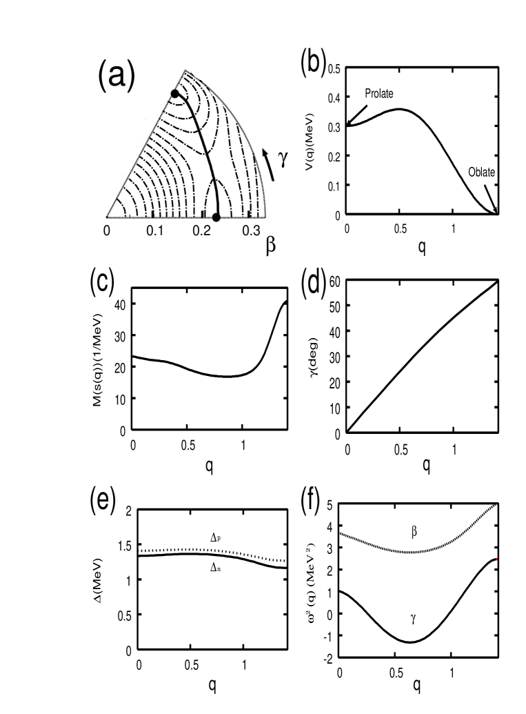
Figure 1: Results of calculation for ⁶⁸Se. (a) The bold curve represents the ASCC path projected onto the $(\beta,\gamma)$ plane, which connects the oblate and the prolate minima designated by filled circles. The contour lines are calculated using the conventional constrained HB method and plotted for every 50 keV. (b) Collective potential $V(q)$ plotted as a function of the collective coordinate $q$. Here the origin of $q$ is chosen to coincide with the prolate local minimum, and its scale is defined such that the collective mass is given by $M(q)=1$. (c) Collective mass $M(s(q))$ with respect to the geometrical length $s(q)$ along the collective path in the $(\beta,\gamma)$ plane, plotted as a function of $q$. (d) The triaxiality parameter $\gamma$ as a function of $q$. (e) Neutron and proton pairing gaps, $\Delta_{n}$ and $\Delta_{p}$, as functions of $q$. (f) Lowest two eigen-frequencies squared (i.e., $\omega^{2}=BC$) of the moving frame RPA, plotted as functions of $q$. These modes at triaxial deformed shapes are more general than the ordinary $\beta$- and $\gamma$-vibrations at the oblate and the prolate limits, and contain both components. The symbols, $\beta$ and $\gamma$, are used, however, in order to indicate the major components of the moving frame RPA modes.

As the $\gamma$ vibrational mode is the lowest-frequency and most collective QRPA mode at the prolate local minimum, we have chosen this mode as an initial condition for solving the basic equations of the ASCC method, and carried out the procedure described in §§ 4.1. We thus obtained the collective path connecting the oblate and prolate local minima in ⁶⁸Se, which is plotted in Fig. 1(a). As we have extracted the collective path in the TDHB phase space, which has huge degrees of freedom, the path drawn in this figure should be regarded as a projection of the collective path onto the ($\beta,\gamma$) plane. Roughly speaking, the collective path goes through the valley that exists in the $\gamma$ direction and connects the oblate and prolate minima. If $\beta$ is treated as a collective coordinate and the oblate and prolate shapes are connected through the spherical point, the variation of the potential energy would be much greater than that along the collective path we obtained. The potential energy curve $V(q)$ along the collective path evaluated using the ASCC method is shown in Fig. 1(b). Since we have defined the scale of the collective coordinate $q$ such that the collective mass is given by $M(q)=B(q)^{-1}=1$ MeV^-1, the collective mass as a function of the geometrical length $s$ along the collective path in the $(\beta,\gamma)$ plane can be defined by

$$M(s(q))=M(q)(\frac{ds}{dq})^{-2}$$ (71)

with $ds^{2}=d\beta^{2}+\beta^{2}d\gamma^{2}$. This quantity is presented in Fig. 1(c) as a function of $q$. The triaxial deformation parameter $\gamma$ is plotted as a function of $q$ in Fig. 1(d). Variations of the pairing gaps, $\Delta_{\tau}(q)$, and of the eigen-frequencies of the moving frame QRPA equations along the collective path are plotted in Figs. 1(e) and 1(f). The solid curve in Fig. 1(f) represents the frequency squared, $\omega^{2}(q)=B(q)C(q)$, given by the product of the inverse mass $B(q)$ and the local stiffness $C(q)$, of the solutions of the moving frame QRPA equations, that corresponds to the $\gamma$-vibration in the oblate and prolate limits. These QRPA solutions determine the infinitesimal generators $\hat{Q}(q)$ and $\hat{P}(q)$ along the collective path. For reference sake, we also present in Fig. 1(f) another solution of the moving frame QRPA equations, which possesses the $\beta$-vibrational character and is irrelevant to the collective path in the case of ⁶⁸Se. Note that the frequency of the $\gamma$-vibrational mode becomes imaginary in the region, $12^{\circ}<\gamma<45^{\circ}$. These results should reveal interesting dynamical properties of the shape coexistence phenomena in ⁶⁸Se. For instance, the large collective mass in the vicinity of $\gamma=60^{\circ}$ (Fig. 1(c)) might increase the stability of the oblate shape in the ground state. Detailed investigation of these quantities as well as solutions of the collective Schrödinger equation will be given in the succeeding paper[84].

5.3 Collective path connecting the oblate and prolate minima in ⁷²Kr

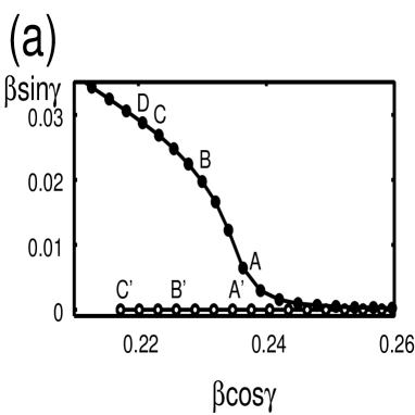
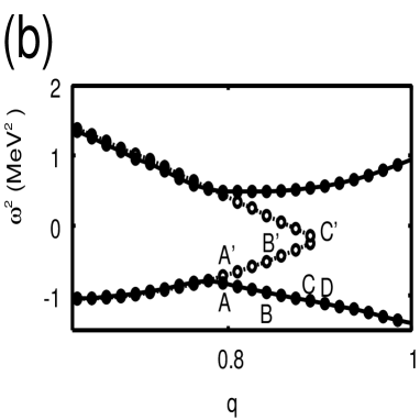
Figure 3: Enlargement of the turn over region of Figs. 2(a) and 2(f) for ⁷²Kr, where the collective path turns into the $\gamma$ direction. The step size $\delta q=0.0157$ and $\varepsilon=0.1$ are used in the numerical calculation. Every steps in $\delta q$ are represented by filled circles and connected by solid lines. The points designated A, B, C, D on the collective path in (a) correspond to those in (b) which displays the squared frequencies, $\omega^{2}$, of the lowest two solutions of the moving frame QRPA equations as functions of the collective coordinate $q$. The open circles represent those obtained in the calculation with $\varepsilon=0$ where the mixing effects between the $K$=$0$ and 2 components are totally ignored. The points designated A’, B’, C’ in the latter calculation correspond to the points A, B, C in the former calculation. In the latter calculation, we cannot get the point corresponding to D because the problem discussed in the text occurs in the numerical algorithm. It was checked that the same collective path is obtained with use of $\delta q=0.0314$ except that the distances between the successive points are doubled.

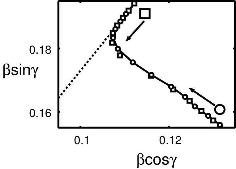
Figure 4: Enlargement of the turn over region of Figs. 2(a) for ⁷²Kr, where the collective path (solid curve) coming from the prolate minimum merges with the $\gamma=60^{\circ}$ axis (dotted line). Every steps in $\delta q$ are represented by open circles and connected by solid lines. For comparison, the result of calculation starting from the oblate minimum and moving in the opposite direction is shown by open squares. Slight deviations from the solid curve indicate the degree of precision of the present numerical calculation. The step size $\delta q=0.0157$ and $\varepsilon=0.1$ are used in both cases. The collective path obtained by these different calculations well agree with each other.

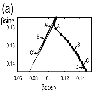
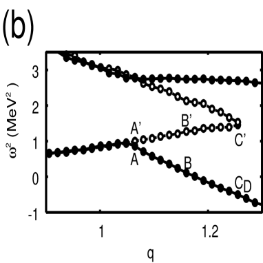
Figure 5: Enlargement of the turn over region of Figs. 2(a) and 2(f) for ⁷²Kr, where the collective path (solid curve) coming from the oblate minimum starts to deviate from the $\gamma=60^{\circ}$ axis (dotted line). The numerical calculation was done starting from the oblate minimum and using the step size $\delta q=0.0157$ and $\varepsilon=0.1$. Every steps in $\delta q$ are represented by filled circles and connected by solid lines. The points designated A, B, C, D on the collective path in (a) correspond to those in (b) which displays the squared frequencies, $\omega^{2}$, of the lowest two solutions of the moving frame QRPA equations as functions of the collective coordinate $q$. Note that the values of $q$ in this figure are measured from the oblate minimum. The open circles represent those obtained in the calculation with $\varepsilon=0$ where the mixing effects between the $K$=$0$ and 2 components are totally ignored. The points designated A’, B’, C’ in the latter calculation correspond to the points A, B, C in the former calculation. In the latter calculation, we cannot get the point corresponding to D because the problem discussed in the text occurs in the numerical algorithm. Slight wiggles along the successive points seen in (b) are due to numerical error, and they indicate the degree of precision of the present numerical calculation. It was checked that the same collective path is obtained with use of $\delta q=0.0314$ except that the distances between the successive points are doubled.

In contrast to ⁶⁸Se, the lowest-frequency QRPA mode is the $\beta$ vibration at the prolate local minimum in ⁷²Kr. Therefore, we have chosen this mode as the initial condition at the prolate minimum and started the procedure of extracting the collective path. Then, the collective path first goes in the direction of the $\beta$ axis on the $(\beta,\gamma)$ plane. As we go along the $\beta$ axis, we eventually encounter a situation that the two solutions of the moving frame QRPA equations compete in energy, and they eventually cross each other. Namely, the character of the solution with the lowest value of $\omega^{2}=BC$ changes from the $\beta$ vibrational to the $\gamma$ vibrational ones at some point on the collective path. If only the solution $\hat{Q}_{1}(q)$ with the lowest value of $\omega^{2}$ at the previous point $q$ is always chosen as an initial guess for $\hat{Q}(q+\delta q)$ in Step 2 of the algorithm described in $\S\S$ 4.1, then the direction of the collective path on the $(\beta,\gamma)$ plane change abruptly from the $\beta$ to the $\gamma$ directions immediately after the crossing point (in the vicinity of the point C’ in Fig. 3 presented below), and the numerical algorithm outlined in $\S\S$ 4.1 fails at this point: During the iterative procedure of solving the moving frame HB equation, we encounter a situation where the overlap $(Q(q),Q(q+\delta q))$ between the infinitesimal generators $\hat{Q}$ at the neighboring points, $q$ and $q+\delta q$, vanishes, because the former possesses $K$=$0$ whereas the latter has $K$=$2$. The numerical algorithm (details of which is described in Appendix B) then stops to work just at this point, where the overlaps $(N_{\tau},Q(q+\delta q))$ also vanish by the same reason. This problem occurs even if we decrease the step size $\delta q$. We find, however, that we can avoid this difficulty by employing a more suitable initial guess for $\hat{Q}(q+\delta q)$. Namely, we take a linear combination of the two solutions, $\hat{Q}_{1}(q)$ and $\hat{Q}_{2}(q)$ at the previous point $q$, $\hat{Q}^{(0)}(q+\delta q)=(1-\varepsilon)\hat{Q}_{1}(q)+\varepsilon\hat{Q}_{2}(q)$, with a small coefficient $\varepsilon$, as an initial guess. This improvement is just for starting the iterative procedure at the next point, $q+\delta q$, on the collective path, so that the self-consistent solution, $\hat{Q}(q+\delta q)$, obtained upon convergence of the iterative procedure, of course, do not depend on the values of $\varepsilon$. For instance, we obtain an axially symmetric solution $\left|\phi(q+\delta q)\right\rangle$ and a generator $\hat{Q}(q+\delta q)$ preserving the $K$ quantum number in the region with $\beta>0.24$ around the prolate minimum, even when we start the iterative procedure using an initial guess for $\hat{Q}(q+\delta q)$ that breaks the axial symmetry. We confirmed that this is indeed the case as long as $\varepsilon$ is a small finite value around 0.1. This special care is needed only near such crossing points (as shown below in Figs. 3-5) where two solutions of the moving frame QRPA equations with different $K$ quantum numbers compete in energy.

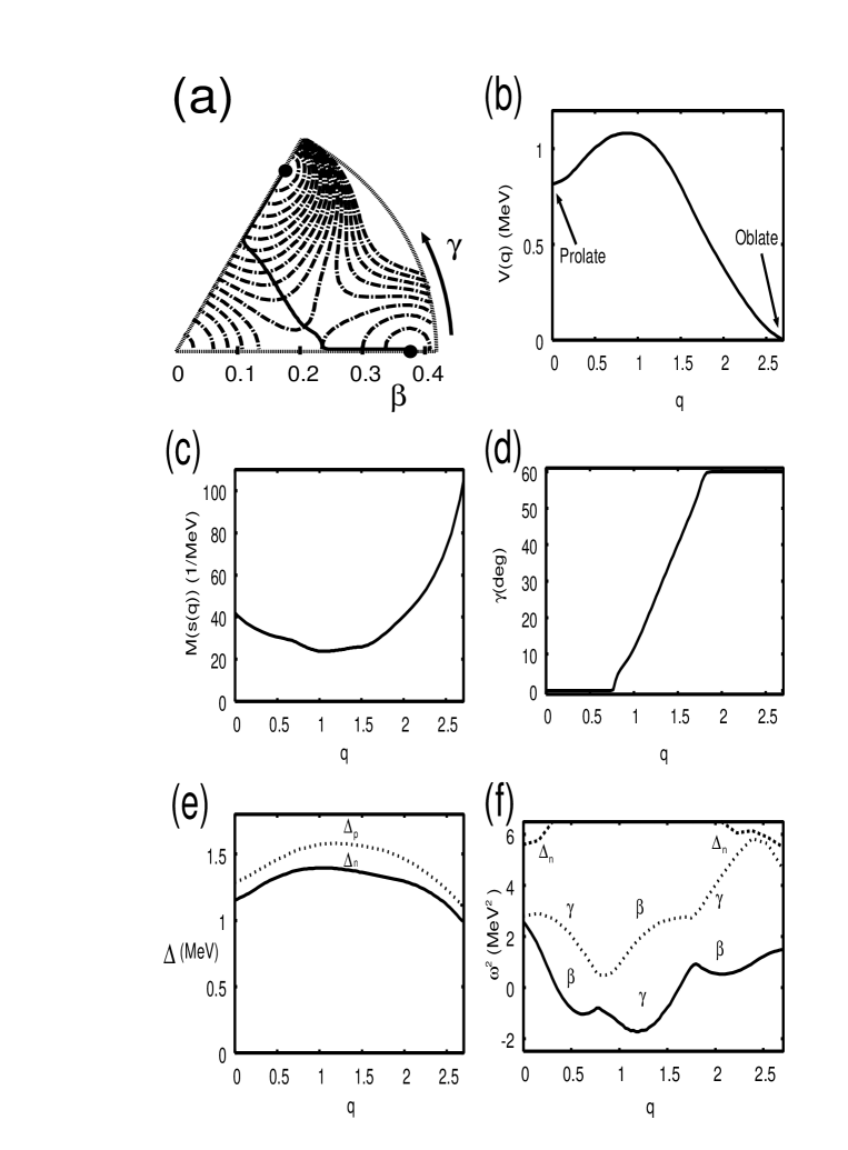
Figure 2: Results of calculation for ⁷²Kr. Notations are the same as in Fig. 1 except for the followings: In (a), the contour lines are plotted for every 100 keV. In (f), the lowest three eigen-frequencies squared (i.e., $\omega^{2}=BC$) of the moving frame RPA, are plotted as functions of $q$. As mentioned in the caption to Fig. 1, these modes at triaxial deformed shapes are more general than the ordinary $\beta$- and $\gamma$-vibrations at the oblate and the prolate limits, and contain both components. The symbols, $\beta$ and $\gamma$, are used, however, in order to indicate the major components of the moving frame RPA modes. Likewise, the symbols $\Delta_{n}$ is used to indicate that the major component is the neutron pairing vibrational mode.

With the improved algorithm mentioned above, we have successfully obtained the smooth deviation of the direction of the collective path from the $\beta$ axis toward the $\gamma$ direction (see Fig. 2(a)). We note that the character of the lowest $\omega^{2}$ solution of the local harmonic equations also gradually changes from the $\beta$ vibrational to the $\gamma$ vibrational ones (see Fig. 2(f)). The details of the turn over region is presented in Fig. 3. One can clearly see in Fig. 3(a) a gradual onset of axial-symmetry breaking in the solutions $\left|\phi(q)\right\rangle$ of the moving frame HB equation. One can also see in Fig. 3(b) an avoided crossing between the lowest two solutions of the moving frame QRPA equations associated with mixing of the components with $K$=$0$ and 2. After the smooth turn to the $\gamma$ direction, the $\gamma$ value increases keeping the $\beta$ value roughly constant, and the collective path eventually approaches to the $\gamma=60^{\circ}$ axis. Then, we again encounter a similar situation. Adopting the improved algorithm, we have confirmed that the character of the lowest $\omega^{2}$ solution smoothly changes, this time, from the $\gamma$ vibrational to the $\beta$ vibrational ones. The collective path thus merges with the $\gamma=60^{\circ}$ axis, and finally reaches the oblate minimum.

We have also carried out the calculation starting from the oblate minimum and proceeded in an inverse way, and obtained the same collective path. This should be regarded as a crucial test of consistency of our calculation. Figure 4 shows the details of this test: The collective path that started from the prolate minimum and turned into the $\gamma$ direction gradually merges with the $\gamma=60^{\circ}$ axis. On the other hand, moving in the opposite direction, we see a gradual onset of axial-symmetry breaking in the collective path that started from the oblate minimum. We see that the two results of calculation for the collective path nicely agree with each other. The importance of taking account of the mixing between the $\beta$- and $\gamma$-vibrational degrees of freedom in solving the moving frame HB and QRPA equations is again demonstrated in Fig. 5, which shows the details of the turn over region from the $\gamma=60^{\circ}$ axis.

Although the collective path drawn in Fig. 2(a) should be regarded as a projection of it onto the $(\beta,\gamma)$ plane, the result of calculation indicates that the collective path runs roughly along the valley in this plane. The potential energy curve $V(q)$, the collective mass $M(s(q))$, variations of the pairing gaps, $\Delta_{\tau}(q)$, are presented in Figs. 2(b), (c), (e), respectively. Their properties are similar to those for ⁶⁸Se. In particular, we notice again a significant increase of $M(s(q))$ in the vicinity of the oblate minimum.

Quite recently, Almehed and Walet studied the oblate-prolate shape coexistence phenomenon in ⁷²Kr by means of an approach similar to the ASCC method but with some additional approximations[80], and found a collective path going from the oblate minimum over a spherical energy maximum into the prolate secondary minimum. We have also obtained such a collective path when we impose the axially symmetry to the solutions $\left|\phi(q)\right\rangle$ of the moving frame HB equation and always use only $K$=$0$ solutions of the moving frame QRPA equations. But, when we relax such symmetry restrictions and follow the lowest $\omega^{2}$ solution of the moving frame QRPA equations, we obtain the collective path presented in Fig. 2, which breaks the axial symmetry. The reason of this disagreement is not clear at present. With their parameters of the P+Q Hamiltonian, they did not encounter the character change of the lowest moving-frame-QRPA mode on the collective path, from the $\beta$ vibrational to the $\gamma$ vibrational ones. However, it is interesting to observe that they in fact encountered the avoided crossing with a $\gamma$-vibrational mode, similar to the one shown in Fig. 2(f), and obtained a collective path that turns into the triaxial plane in their calculation for states with angular momentum $I=2$.

6 Concluding Remarks

We have applied the ASCC method to the oblate-prolate shape coexistence phenomena in ⁶⁸Se and ⁷²Kr. It was found that the self-consistent collective paths run approximately along the valley connecting the oblate and prolate local minima in the collective potential energy landscape. This is the first time that the self-consistent collective paths between the oblate and prolate minima have been obtained for realistic situations starting from the microscopic P+Q Hamiltonian. Recently, the generator coordinate method has often been used to describe a variety of shape coexistence phenomena, with $\beta$ employed as the generator coordinate[47, 48]. The triaxial shape vibrational degrees of freedom are also ignored in the extensive variational calculations by Tübingen group[49, 50]. The result of the ASCC calculation, however, strongly indicates the necessity of taking into account the $\gamma$ degree of freedom, at least for the purpose of describing the oblate-prolate shape coexistence in ⁶⁸Se and ⁷²Kr. In order to evaluate the mixing effects between the oblate and prolate shapes taking into account the triaxial deformation dynamics, we have to quantize the classical collective Hamiltonian obtained in this paper and solve the resulting collective Schrödinger equation. This will be the subject of the succeeding paper[84].

Appendix A Explicit expressions of the quasiparticle matrix elements

Combining the successive Bogoliubov transformations, (3.8) and (3.18), the quasiparticles, $a_{\mu}^{{\dagger}}(q)$ and $a_{\mu}(q)$, associated with the state $|\phi(q)\rangle$, can be written in terms of the nucleon operator, $d_{k}^{{\dagger}}$ and $d_{\bar{k}}$, as

$$\left(\begin{array}[]{c}a_{\mu}^{{\dagger}}(q)\\ a_{\bar{\mu}}(q)\end{array}\right)=\sum_{k}\left(\begin{array}[]{cc}U_{\mu k}(q)&V_{\mu\bar{k}}(q)\\ V_{\bar{\mu}k}(q)&U_{\bar{\mu}\bar{k}}(q)\end{array}\right)\left(\begin{array}[]{c}d_{k}^{{\dagger}}\\ d_{\bar{k}}\end{array}\right)$$ (72)

Making use of the inverse transformation,

$$\left(\begin{array}[]{c}d_{k}^{{\dagger}}\\ d_{\bar{k}}\end{array}\right)=\sum_{\mu}\left(\begin{array}[]{cc}U_{k\mu}(q)&V_{k\bar{\mu}}(q)\\ V_{\bar{k}\mu}(q)&U_{\bar{k}\bar{\mu}}(q)\end{array}\right)\left(\begin{array}[]{c}a_{\mu}^{{\dagger}}(q)\\ a_{\bar{\mu}}(q)\end{array}\right),$$ (73)

one can easily derive the explicit expressions of the expectation values and the matrix elements of the operators, ${\hat{F}}_{s}^{(\pm)}$, appearing in Eq. (30):

$$\left\langle\phi(q)\right|{\hat{F}}_{s=1,2}^{(+)}\left|\phi(q)\right\rangle = -2\sum_{\mu}\sum_{k}(k{\bar{k}}|A_{\tau=n,p}^{(+)}|0)U_{k\mu}(q)V_{\bar{k}\mu}(q),$$

$$F_{s=1,2}^{(\pm)}(\mu\bar{\nu}) = \sum_{k}(k{\bar{k}}|A_{\tau=n,p}^{(\pm)}|0)\Big{(}U_{k\mu}(q)U_{\bar{k}\bar{\nu}}(q)\pm V_{k\bar{\nu}}(q)V_{\bar{k}\mu}(q)\Big{)},$$

$$F_{B,s=1,2}^{(\pm)}(\mu\nu) = \sum_{k}(k{\bar{k}}|A_{\tau=n,p}^{(\pm)}|0)\Big{(}U_{k\mu}(q)V_{\bar{k}\nu}(q)\pm U_{k\nu}(q)V_{\bar{k}\mu}(q)\Big{)},$$

$$\left\langle\phi(q)\right|{\hat{F}}_{s=3,5}^{(+)}\left|\phi(q)\right\rangle = 2\sum_{\bar{\mu}}\sum_{kl}(k|D_{2,K=0,2}^{(+)}|l)V_{k\bar{\mu}}(q)V_{l\bar{\mu}}(q),$$

$$F_{s=3,5}^{(+)}(\mu\bar{\nu}) = \sum_{kl}(k|D_{2,K=0,2}^{(+)}|l)\Big{(}U_{k\mu}(q)V_{l\bar{\nu}}(q)+U_{k\nu}(q)V_{l\bar{\mu}}(q)\Big{)},$$

$$F_{B,s=3,5}^{(+)}(\mu\nu) = \sum_{kl}(k|D_{2,K=0,2}^{(+)}|l)\Big{(}U_{k\mu}(q)U_{l\nu}(q)-V_{k\bar{\nu}}(q)V_{l\bar{\mu}}(q)\Big{)},$$ (74)

The expectation values of the anti-Hermitian operators, $A_{\tau=n,p}^{(-)}$, vanish. The quantities, $(k|D_{2K}^{(+)}|l)$, etc., appearing in the above expressions denote matrix elements between the single-particle states defined by Eq. (13):

$$(k|D_{2K}^{(+)}|l) \equiv (0|d_{k}D_{2K}^{(+)}d_{l}^{{\dagger}}|0),$$

$$(k\bar{k}|A_{\tau}^{(\pm)}|0) \equiv (0|d_{\bar{k}}d_{k}A_{\tau}^{(\pm)}|0),~{}~{}~{}{\rm etc}.,$$ (75)

where $|0)$ is the vacuum for the nucleon operators $(d^{{\dagger}},d)$. The matrix elements of the Bogoliubov transformations, (A.1) and (A.2), possess the following symmetries:

$$U_{\mu k}=U_{\bar{\mu}\bar{k}}=U_{k\mu}=U_{\bar{k}\bar{\mu}},~{}~{}V_{\mu\bar{k}}=-V_{\bar{\mu}k}=V_{k\bar{\mu}}=-V_{\bar{k}\mu}.$$ (76)

It is also easily seen that equalities,

$$(\bar{k}|D_{2,K=0,2}^{(+)}|\bar{l})=(k|D_{2,K=0,2}^{(+)}|l),$$ (77)

$$~{}~{}~{}F_{B,s}^{(\pm)}(\bar{\mu}\bar{\nu})=F_{B,s}^{(\pm)}(\mu\nu),~{}~{}~{}F_{B,s}^{(\pm)}(\nu\mu)=\pm F_{B,s}^{(\pm)}(\mu\nu),$$ (78)

hold for the pairing and quadrupole operators, $\{A_{n}^{(\pm)},A_{p}^{(\pm)},D_{20}^{(+)},D_{22}^{(+)}\}$, under consideration. The expectation values, $\left\langle\phi(q)\right|{\hat{N}}_{\tau}\left|\phi(q)\right\rangle$, and the matrix elements, $N_{\tau}(\mu)$ and $N_{B,\tau}(\mu)$, of the neutron and proton number operators are readily obtained from those of ${\hat{F}}_{s=3}^{(+)}$ by replacing $(k|D_{20}^{(+)}|l)$ with $\delta_{kl}$, and restricting the sum over the single-particle index $k$ to neutrons or protons.

Appendix B Solving the moving frame HB equation

We solve the moving frame HB equation using a method similar to the imaginary time method[85]. Let $\left|\phi^{(i)}(q)\right\rangle$ be the state vector in the iterative step $i$. We first calculate the mean-field Hamiltonian associate with it:

$${\hat{h}}^{(i)}(q) = \sum_{k}\epsilon_{k}(d_{k}^{{\dagger}}d_{k}+d_{\bar{k}}^{{\dagger}}d_{\bar{k}})-\sum_{s}\kappa_{s}\langle{\hat{F}}_{s}^{(+)}\rangle^{(i)}{\hat{F}}_{s}^{(+)},$$

$$\langle{\hat{F}}_{s}^{(+)}\rangle^{(i)} \equiv \left\langle\phi^{(i)}(q)\right|{\hat{F}}_{s}^{(+)}\left|\phi^{(i)}(q)\right\rangle.$$ (79)

Using the quasiparticle operators $b_{\mu}^{(i){\dagger}}$ and $b_{\mu}^{(i)}$ defined by

$$b_{\mu}^{(i)}\left|\phi^{(i)}(q)\right\rangle=0,$$ (80)

we then generate a state vector in the $(i+1)$ step as

$$\left|{\phi^{(i+1)}(q)}\right\rangle \equiv \exp{\hat{X}^{(i+1)}}\left|{\phi^{(i)}(q)}\right\rangle$$

$${\hat{X}^{(i+1)}}= - \varepsilon\Big{(}{\hat{h}}^{(i)}(q)-\sum_{\tau}\lambda_{\tau}^{(i+1)}(q){\hat{N}}_{\tau}-\mu^{(i+1)}(q){\hat{Q}}(q)\Big{)}_{+}$$ (81)

$$+ \varepsilon\Big{(}{\hat{h}}^{(i)}(q)-\sum_{\tau}\lambda_{\tau}^{(i+1)}(q){\hat{N}}_{\tau}-\mu^{(i+1)}(q){\hat{Q}}(q)\Big{)}_{-}$$

$$\equiv \sum_{\mu\bar{\nu}}x_{\mu\bar{\nu}}^{(i+1)}\Big{(}{\mbox{\boldmath$X$}_{\mu\bar{\nu}}^{(i){\dagger}}-\mbox{\boldmath$X$}_{\mu\bar{\nu}}^{(i)}}\Big{)},$$

where $\varepsilon$ is a small parameter,

$$\mbox{\boldmath$X$}_{\mu\bar{\nu}}^{(i){\dagger}}=b_{\mu}^{(i){\dagger}}b_{\bar{\nu}}^{(i){\dagger}},~{}~{}~{}\mbox{\boldmath$X$}_{\mu\bar{\nu}}^{(i)}=b_{\bar{\nu}}^{(i)}b_{\mu}^{(i)},$$ (82)

and the subscripts, $+$ and $-$, denote the two-quasiparticle creation and annihilation parts of the operator in the parenthesis, respectively. It should be noted that, in contrast to the conventinal imaginary time method, the unitary operator, $\exp{\hat{X}^{(i+1)}}$, is used here so that the normalization is preserved during the iteration. The Lagrange multipliers $\lambda_{\tau}^{(i+1)}(q)$ and $\mu^{(i+1)}(q)$ are determined by the constraint equations,

$$\left\langle{\phi^{(i+1)}(q)}\right|{\hat{N}}_{\tau}{\left|\phi^{(i+1)}(q)\right\rangle} = N_{\tau}^{(0)}$$

$$\left\langle{\phi^{(i+1)}(q)}\right|{\hat{Q}}(q-\delta q){\left|\phi^{(i+1)}(q)\right\rangle} = \delta q,$$ (83)

where $N_{n}^{(0)}$ and $N_{p}^{(0)}$ are the neutron and proton numbers of the nucleus under consideration. Similar but slightly different constraints are utilized by Almehed and Walet[79]. Expanding the left-hand sides up to first order in $x^{(i+1)}$, we obtain equations determining them:

$$\left(\begin{array}[]{ccc}(N_{n},N_{n})&(N_{n},N_{p})&(N_{n},Q(q))\\ (N_{p},N_{n})&(N_{p},N_{p})&(N_{p},Q(q))\\ (Q(q-\delta q),N_{n})&(Q(q-\delta q),N_{p})&(Q(q-\delta q),Q(q))\end{array}\right)\left(\begin{array}[]{c}\lambda_{n}^{(i+1)}(q)\\ \lambda_{p}^{(i+1)}(q)\\ \mu^{(i+1)}(q)\end{array}\right)$$ (90)

$$=\left(\begin{array}[]{c}(N_{n}^{(0)}-\langle{\hat{N}}_{n}\rangle^{(i)})/2\varepsilon+(h^{(i)}(q),N_{n})\\ (N_{p}^{(0)}-\langle{\hat{N}}_{p}\rangle^{(i)})/2\varepsilon+(h^{(i)}(q),N_{p})\\ (\delta q-\langle{\hat{Q}}(q-\delta q)\rangle^{(i)})/2\varepsilon+(h^{(i)}(q),Q(q-\delta q)),\end{array}\right),$$ (94)

where the quantities, $(N_{\tau},N_{\tau^{\prime}}),(N_{\tau},Q(q))$ etc., are defined by (3.33), except that the coefficients, $N_{\tau}(\mu),Q_{\mu\bar{\nu}}(q)$ etc., involved in these quantities are here defined with respect to the two-quasiparticle creation and annihilation operators, $\mbox{\boldmath$X$}_{\mu\bar{\nu}}^{(i){\dagger}}$ and $\mbox{\boldmath$X$}_{\mu\bar{\nu}}^{(i)}$. Using the state vector $\left|{\phi^{(i+1)}(q)}\right\rangle$, we calculate the mean-field Hamiltonian ${\hat{h}}^{(i+1)}(q)$ in the $(i+1)$ step, and repeat the above procedure until convergence is attained. The mean-field Hamiltonian thus obtained takes the following form:

$${\hat{h}}_{M}(q) = {\hat{h}}(q)-\sum_{\tau}\lambda_{\tau}(q){\hat{N}}_{\tau}-\mu(q){\hat{Q}}(q)$$ (95)

$$= \left\langle\phi(q)\right|\hat{h}_{M}(q)\left|\phi(q)\right\rangle+\sum_{\mu\nu}h_{\mu\nu}(q)\Big{(}b_{\mu}^{{\dagger}}(q)b_{\nu}(q)+b_{\bar{\mu}}^{{\dagger}}(q)b_{\bar{\nu}}(q)\Big{)}.$$

Finally we introduce the quasiparticle operators, $a^{{\dagger}}_{\mu}(q)$ and $a_{\mu}(q)$, that diagonalize ${\hat{h}}_{M}(q)$:

$${\hat{h}}_{M}(q)=\left\langle\phi(q)\right|\hat{h}_{M}(q)\left|\phi(q)\right\rangle+\sum_{\mu}E_{\mu}(q)\Big{(}a_{\mu}^{{\dagger}}(q)a_{\mu}(q)+a_{\bar{\mu}}^{{\dagger}}(q)a_{\bar{\mu}}(q)\Big{)}.$$ (96)

It is easy to see that $\mu(q)=\partial V/\partial q$. In actual calculations, the above procedure is a part of the double iterative algorithm described in section 4. Namely, we carry out the above iterative procedure using the constraint operator ${\hat{Q}}(q)^{(n)}$ that is obtained in the $n$-th iteration step determining the infinitesimal generators, ${\hat{Q}}(p)$ and ${\hat{P}}(q)$.

References

• [1] P. Ring and P. Schuck, The Nuclear Many-Body Problem (Springer-Verlag, 1980).
• [2] J.-P. Blaizot and G. Ripka, Quantum Theory of Finite Systems (The MIT press, 1986).
• [3] A. Klein and E.R. Marshalek, Rev. Mod. Phys. 63 (1991), 375.
• [4] G. Do Dang, A. Klein, and N.R. Walet, Phys. Rep. 335 (2000), 93.
• [5] A. Kuriyama, K. Matsuyanagi, F. Sakata, K. Takada, and M. Yamamura (eds), Prog. Theor. Phys. Suppl. 141 (2001).
• [6] D.J. Rowe and R. Bassermann, Canad. J. Phys. 54 (1976), 1941.
• [7] K. Goeke, Nucl. Phys. A 265 (1976), 301.
• [8] F. Villars, Nucl. Phys. A 285 (1977), 269.
• [9] T. Marumori, Prog. Theor. Phys. 57 (1977), 112.
• [10] M. Baranger and M. Veneroni, Ann. of Phys. 114 (1978), 123.
• [11] K. Goeke and P.-G. Reinhard, Ann. of Phys. 112 (1978), 328.
• [12] T. Marumori, T. Maskawa, F. Sakata, and A.Kuriyama, Prog. Theor. Phys. 64 (1980), 1294.
• [13] M.J. Giannoni and P. Quentin, Phys. Rev. C 21 (1980), 2060.
• [14] J. Dobaczewski and J. Skalski, Nucl. Phys. A 369 (1981), 123.
• [15] K. Goeke, P.-G. Reinhard, and D.J. Rowe, Nucl. Phys. A 359 (1981), 408.
• [16] A.K. Mukherjee and M.K. Pal, Phys. Lett. B 100 (1981), 457; Nucl. Phys. A 373 (1982), 289.
• [17] D. J. Rowe, Nucl. Phys. A 391 (1982), 307.
• [18] C. Fiolhais and R.M. Dreizler, Nucl. Phys. A 393 (1983), 205.
• [19] K. Goeke, F. Grümmer, and P.-G. Reinhard, Ann. of Phys. 150 (1983), 504.
• [20] A. Kuriyama and M. Yamamura, Prog. Theor. Phys. 70 (1983), 1675; 71 (1984), 122.
• [21] M. Yamamura, A. Kuriyama, and S. Iida, Prog. Theor. Phys. 71 (1984), 109.
• [22] M. Matsuo and K. Matsuyanagi, Prog. Theor. Phys. 74 (1985), 288.
• [23] M. Matsuo, Prog. Theor. Phys. 76 (1986), 372.
• [24] Y.R. Shimizu and K. Takada, Prog. Theor. Phys. 77 (1987), 1192.
• [25] M. Yamamura and A. Kuriyama, Prog. Theor. Phys. Suppl. 93 (1987), 1.
• [26] N.R. Walet, G. Do Dang, and A. Klein, Phys. Rev. C 43 (1991), 2254.
• [27] A. Klein, N.R. Walet, and G. Do Dang, Ann. of Phys. 208 (1991), 90.
• [28] K. Kaneko, Phys. Rev. C 49 (1994), 3014.
• [29] T. Nakatsukasa and N.R. Walet, Phys. Rev. C 57 (1998), 1192.
• [30] T. Nakatsukasa and N.R. Walet, Phys. Rev. C 58 (1998), 3397.
• [31] J. Libert, M. Girod and J.-P. Delaroche, Phys. Rev. C 60 (1999), 054301.
• [32] E.Kh. Yuldashbaeva, J. Libert, P. Quentin and M. Girod, Phys. Lett. B 461 (1999), 1.
• [33] T. Nakatsukasa, N.R. Walet, and G. Do Dang, Phys. Rev. C 61 (2000), 014302.
• [34] J.L. Wood, K. Heyde, W. Nazarewicz, M. Huyse, and P. van Duppen, Phys. Rep. 215 (1992), 101.
• [35] W. Nazarewicz, Phys. Lett. B 305 (1993), 195.
• [36] W. Nazarewicz, Nucl. Phys. A 557 (1993), 489c.
• [37] N. Tajima, H. Flocard, P. Bonche, J. Dobaczewski, and P.-H. Heenen, Nucl. Phys. A 551 (1993), 409.
• [38] P. Bonche, E. Chabanat, B.Q. Chen, J. Dobaczewski, H. Flocard, B. Gall, P.H. Heenen, J. Meyer, N. Tajima, and M.S. Weiss, Nucl. Phys. A 574 (1994), 185c.
• [39] P.-G. Reinhard, D.J. Dean, W. Nazarewicz, J. Dobaczewski, J.A. Maruhn, and M.R. Strayer, Phys. Rev. C 60 (1999), 014316.
• [40] A.N. Andreyev et al., Nature 405 (2000) 430; Nucl. Phys. A 682 (2001), 482c.
• [41] S. M. Fischer et al., Phys. Rev. Lett. 84 (2000), 4064; Phys. Rev. C 67 (2003), 064318.
• [42] E. Bouchez et al., Phys. Rev. Lett. 90 (2003), 082502.
• [43] R.R. Rodríguez-Guzmán, J.L. Egido, and L.M. Robledo, Phys. Rev. C 62 (2000), 054319; C 65 (2002), 024304 G C 69 (2004), 054319.
• [44] J.L. Egido, and L.M. Robledo, and R.R. Rodríguez-Guzmán, Phys. Rev. Lett. 93 (2004), 082502.
• [45] R.R. Chasman, J.L. Egido, L.M. Robledo, Phys. Lett. B 513 (2001), 325.
• [46] T. Nikšić, D. Vretenar, P. Ring, and G.A. Lalazissis, Phys. Rev. C 65 (2002), 054320.
• [47] T. Duguet, M. Bender, P. Bonche, and P.-H. Heenen, Phys. Lett. B 559 (2003), 201.
• [48] M. Bender, P. Bonche, T. Duguet, and P.-H. Heenen, Phys. Rev. C 69 (2004), 064303.
• [49] A. Petrovici, K.W. Schmid, and A. Faessler, J.H. Hamilton, and A.V. Ramayya, Prog. in Part. Nucl. Phys. 43 (1999), 485.
• [50] A. Petrovici, K.W. Schmid, and A. Faessler, Nucl. Phys. A 665 (2000) 333; A 710 (2002), 246.
• [51] R. Fossion, K. Heyde, G. Thiamova, and P. Van Isacker, Phys. Rev. C 67 (2003), 024306.
• [52] A. Frank, P. Van Isacker, and C.E. Vargas, Phys. Rev. C 69 (2004), 034323.
• [53] C.D. Dracoulis et al. Phys. Rev. C 69 (2004), 054318.
• [54] K. Kaneko, M. Hasegawa, and T. Mizusaki, Phys. Rev. C 66 (2002), 051306(R); preprint nucl-th/0410046.
• [55] M. Hasegawa, K. Kaneko, T. Mizusaki, and S. Tazaki, Phys. Rev. C 69 (2004), 034324.
• [56] M. Hasegawa, K. Kaneko, and T. Mizusaki, preprint nucl-th/0408062; nucl-th/0408063.
• [57] Y. Sun, Eur. Phys. J. A 20 (2004), 133.
• [58] M. Matsuo, Prog. Theor. Phys. 72 (1984), 666.
• [59] M. Matsuo and K. Matsuyanagi, Prog. Theor. Phys. 74 (1985), 1227; 76 (1986), 93; 78 (1987) 591.
• [60] M. Matsuo, Y. R. Shimizu, and K. Matsuyanagi, Proceedings of The Niels Bohr Centennial Conf. on Nuclear Structure, ed. R. Broglia, G. Hagemann and B. Herskind (North-Holland, 1985), p. 161.
• [61] K. Takada, K. Yamada, and H. Tsukuma, Nucl. Phys. A 496 (1989), 224.
• [62] K. Yamada, K. Takada, and H. Tsukuma, Nucl. Phys. A 496 (1989), 239.
• [63] K. Yamada and K. Takada, Nucl. Phys. A 503 (1989), 53.
• [64] H. Aiba, Prog. Theor. Phys. 84 (1990), 908.
• [65] K. Yamada, Prog. Theor. Phys. 85 (1991), 805; 89 (1993), 995.
• [66] J. Terasaki, T. Marumori, and F. Sakata, Prog. Theor. Phys. 85 (1991), 1235.
• [67] J. Terasaki, Prog. Theor. Phys. 88 (1992), 529; 92 (1994), 535.
• [68] M. Matsuo, in New Trends in Nuclear Collective Dynamics, (Springer-Verlag, 1992), eds. Y. Abe, H. Horiuchi and K. Matsuyanagi, p.219.
• [69] Y.R. Shimizu and K. Matsuyanagi, Prog. Theor. Phys. Suppl. 141 (2001), 285.
• [70] M. Matsuo, T. Nakatsukasa, and K. Matsuyanagi, Prog. Theor. Phys. 103 (2000), 959.
• [71] M. Kobayasi, T. Nakatsukasa, M. Matsuo and K. Matsuyanagi, Prog. Theor. Phys. 110 (2003), 65.
• [72] K. Matsuyanagi, Prog. Theor. Phys. 67 (1982) 1141; Proceedings of the Nuclear Physics Workshop, Trieste, 5-30 Oct. 1981. ed. C.H. Dasso, R.A. Broglia and A. Winther (North-Holland, 1982), p.29.
• [73] Y. Mizobuchi, Prog. Theor. Phys. 65 (1981), 1450.
• [74] T. Suzuki and Y. Mizobuchi, Prog. Theor. Phys. 79 (1988), 480.
• [75] T. Fukui, M. Matsuo and K. Matsuyanagi, Prog. Theor. Phys. 85 (1991), 281.
• [76] M. Baranger and K. Kumar, Nucl. Phys. 62 (1965) 113; A 110 (1968), 529; A 122 (1968), 241; A 122 (1968), 273.
• [77] M. Baranger and K. Kumar, Nucl. Phys. A 110 (1968), 490.
• [78] D. R. Bes and R. A. Sorensen, Advances in Nuclear Physics (Prenum Press, 1969), vol. 2, p. 129.
• [79] D. Almehed and N. R. Walet, Phys. Rev. C 69 (2004), 024302.
• [80] D. Almehed and N. R. Walet, preprint nucl-th/0406028.
• [81] M. Kobayasi, T. Nakatsukasa, M. Matsuo and K. Matsuyanagi, Prog. Theor. Phys. 112 (2004), 363.
• [82] M. Yamagami, K. Matsuyanagi and M. Matsuo, Nucl. Phys. A 693 (2001), 579.
• [83] T. Bengtsson and I. Ragnarsson, Nucl. Phys. A 436 (1985), 14.
• [84] M. Kobayasi, T. Nakatsukasa, M. Matsuo and K. Matsuyanagi, in preparation.
• [85] K.T.R. Davies, H. Flocard, S. Krieger, and M.S. Weiss, Nucl. Phys. A 342 (1980), 111.