Electromagnetic strength of neutron and proton single-particle halo nuclei
Abstract
Electromagnetic strength functions of halo nuclei exhibit universal features that can be described in terms of characteristic scale parameters. For a nucleus with nucleon+core structure the reduced transition probability, as determined, e.g., by Coulomb dissociation experiments, shows a typical shape that depends on the nucleon separation energy and the orbital angular momenta in the initial and final states. The sensitivity to the final-state interaction (FSI) between the nucleon and the core can be studied systematically by varying the strength of the interaction in the continuum. In the case of neutron+core nuclei analytical results for the reduced transition probabilities are obtained by introducing the effective-range expansion. The scaling with the relevant parameters is found explicitly. General trends are observed by studying several examples of neutron+core and proton+core nuclei in a single-particle model assuming Woods-Saxon potentials. Many important features of the neutron halo case can be obtained from a square-well model. Rather simple analytical formulas are found. The nucleon-core interaction in the continuum affects the determination of astrophysical S factors at zero energy in the method of asymptotic normalisation coefficients (ANC). It is also relevant for the extrapolation of radiative capture cross sections to low energies.
keywords:
halo nuclei , electromagnetic transitions , effective-range approximation , scaling laws , final-state interaction , sum rules , ANC method , radiative capturePACS:
21.10.Pc , 21.10.Ky , 25.20.-x , 25.40.Lw , 27.20.+n1 Introduction
Light exotic nuclei are available as secondary beams at various radioactive beam facilities all over the world. These unstable nuclei are generally weakly bound with few, if any, bound excited states. They have been studied extensively in recent years by electromagnetic excitation with the help of the Coulomb breakup method [1, 2, 3, 4, 5]. For low orbital angular momenta of the lowest bound valence nucleon an extended diffuse density distribution, a halo, develops resulting in a large size of the nucleus [6, 7, 8, 9, 10]. Simultaneously, electromagnetic transitions to the continuum with large strength are observed at low energies. Properties of stable nuclei have successfully been investigated by electromagnetic excitation in photonuclear reactions as well as in heavy ion collisions for a long time. Their electromagnetic strength functions are dominated by the giant resonances high in the continuum.
Nuclei close to the neutron and proton drip lines often exhibit a pronounced nucleon+core structure that is well described by single-particle models with appropriately chosen potentials. In a microscopic shell-model study [11] strong low-lying dipole strength in neutron-rich 14Be and proton-rich 13O was observed to originate from loosely-bound extended single-particle wave functions. These extended wave functions were obtained by adjusting the potential depth in order to reproduce the empirical binding energies. In order to study low-lying strength theoretically, such a feature has to be added to the ab-initio microscopic approaches. A comparison of strength functions deduced from experiment with theoretical predictions from single-particle models is used to extract spectroscopic factors or asymptotic normalization coefficients (ANC). They can be compared to more elaborated nuclear models. However, the importance of effects from the interaction between the nuclei in the final state has to be assessed in order to obtain reliable information from experimental data. Both the shape and the absolute magnitude of the strength function can be affected. This will also have consequences for the application of sum rules that relate the total excitation strength to the properties of the ground state.
The relevant matrix elements for the electromagnetic transition to the continuum at low energies are esssentially determined by the asymptotics of the bound-state and continuum wave functions of halo nuclei. This allows to study systematically the effects of the final-state interaction (FSI) without the necessity to introduce sophisticated nuclear structure models. Magnetic contributions to the continuum transitions are usually much weaker than electric transitions, except for the deuteron breakup at low energies [12] and for the excitation of resonances. We will limit ourselves to the discussion of direct electric transitions to the continuum, with emphasis on transitions, but the search for low-lying strength and its theoretical description [13] remains an interesting challenge for future studies.
The nuclear interaction between the nucleon and the core in the electromagnetic breakup of an exotic nucleus is responsible for the binding of the nucleus . However, it also affects the structure of the continuum (usually in partial waves with different values) even if there are no resonances observed at low excitation energies. In the experimental analysis of neutron+core breakup reactions it is often neglected and a plane wave is assumed in the final state of the system. The interaction between and also appears in the final state of the photo-dissociation reaction or in the initial state of the radiative capture reaction . Thus, the interaction can affect the energy dependence of the astrophysical S factor of the radiative capture reaction that is used to extrapolate experimental data to zero energy. Similarly, the strength of the interaction enters into the calculation of the zero-energy S factor from asymptotic normalization coefficients (ANCs) that are determined experimentally from transfer reactions in the ANC method, see, e.g., [14, 15, 16, 17].
Experimentally observed excitation functions of exotic nuclei show an approximately universal shape when plotted as a function of appropriately scaled variables [18, 19, 20, 21]. They are dominated by direct transitions to the continuum with only few resonances and simple scaling laws apply. The nuclear structure in the initial and final state depends only on a limited number of relevant quantities that contain all the structural information that is accessible at low energies. Details of the nuclear interaction are not resolved at this low energy scale. The interaction between the fragments leads to a change of the transition strength when compared to the case without nuclear interaction. The actual nuclear potential is often not well constrained since extrapolations of the corresponding systematic optical potentials, e.g. [22], from nuclei in the valley of stability to unstable nuclei are questionable. The effect of the continuum interaction was studied before only in selected cases. E.g., it was found that the -wave ground state to -wave continuum transition in the case of 11Be is much less affected by the potential in the final state than the transition in 13C [18, 19].
At low energies the effect of the nuclear potential is conveniently described by the effective-range expansion [23, 24], with the scattering length and the effective range as the main parameters. An effective-range approach for the FSI in electromagnetic excitations was introduced in [25] and applied to the breakup of 11Be. Recently, the same method was applied to the description of electromagnetic dipole strength in 23O [26]. Here, we will discuss this approach in much more detail. A systematic study for various transitions will shed some additional light on the sensitivity to the interaction in the continuum. We want to expose the dependence on the binding energy of the nucleon and on the angular momentum quantum numbers. Our approach extends the familiar textbook case of the deuteron [13], that can be considered as the prime example of a halo nucleus, to arbitrary nucleon+core systems.
Our effective-range approach is closely related to effective field theories that are nowadays used for the description of the nucleon-nucleon system and halo nuclei [27, 28, 29]. (The deuteron, the only bound state in the nucleon-nucleon system, can be considered as a good example of a halo nucleus). The characteristic low-energy parameters are linked to QCD in systematic expansions. Similar methods are also used in the study of exotic atoms (, , , …) in terms of effective-range parameters in Ref. [30]. The close relation of effective field theory to the effective-range approach for hadronic atoms was discussed in Ref. [31]. In our approach these constants are treated as free parameters. It is not our aim to relate them to the underlying microscopic description. Aspects of the many-body physics are summarized, e.g., in terms of spectroscopic factors or asymptotic normalization coefficients.
We also investigate in detail a specific model, the square well potential. It has great merits: it can be solved analytically, it shows the main characteristic features and it leads to rather simple and transparent formulas where some of them seem to be new. These explicit results can be compared to our general results for low energies (effective-range approach) and also to Woods-Saxon models.
This paper is organized as follows. A nucleon+core potential model for halo nuclei is introduced in section 2. The relevant scaling parameters are defined in subsection 2.1 and scaling laws for the the probabilities to find the nucleon inside the range of the nuclear potential are discussed for bound and scattering states in subsection 2.2. The scaling of the root-mean-square radius serves as another indication for the halo nature of the bound state. The reduced transition probabilities for the breakup of a nucleon+core nucleus are calculated in subsection 2.3 for electric transitions with multipolarity . They only depend on the asymptotic normalization of the bound state wave function and on radial integrals with the asymptotic wave functions since the radial integrals are dominated by the contribution from outside the nuclear potential. In the square-well model explicit expressions for the ratio of the interior to the exterior contributions are derived. An alternative calculation of transition integrals with the help of a commutator relation is presented in subsection 2.4. The strength functions are related to cross sections of photo-nuclear reactions in subsection 2.5 and the high-energy behaviour is discussed. The effect of the nucleon-core potential is considered in subsection 2.6. The effective-range expansion allows to parametrize the effects of the continuum interaction in a suitable way to study systematically its influence on the transition strength. In Section 3 the reduced transition probabilities are expressed in terms of characteristic shape functions that depend on certain reduced integrals. The dependence of the shape functions on the scaling parameters is studied in various limits. Systematic variations of the shape functions are discussed for neutron+core systems in subsections 3.1 and 3.2 without and with FSI, respectively, where analytical results are obtained. Proton+core systems are treated numerically in subsection 3.3. The relation of the total excitation strength to the properties of the bound state with the help of sum rules is considered in section 4. The findings of the model with asymptotic wave functions are corroborated in more realistic calculations using wave function generated from Woods-Saxon potentials in section 5. The implication of the nucleon-core interaction in the continuum state on the ANC method is discussed in section 6. We close with a summary and conclusions. The appendix contains detailed derivations and explicit expressions of our analytic calculations.
2 Nucleon+core model
Exotic nuclei close to the driplines often exhibit a pronounced structure with a nucleon (proton or neutron) weakly bound to a core . They are often well described by simple single-particle models that are able to explain the basic features of low-energy excitations. For small separation energies of the nucleon and low orbital angular momenta the exotic nucleus develops a proton or neutron halo where the nucleon wave function extends to large radii and there is a large probability of finding the nucleon outside the classically allowed region of the potential . Matrix elements for electromagnetic transitions only depend on a small number of characteristic scaling parameters.
2.1 Scaling parameters of halo nuclei
The main scale is set by the nucleon separation energy () that is related to an inverse decay length
| (1) |
of the bound state with the reduced mass . It becomes very small for typical halo nuclei with small binding energies. The scattering state is characterized by the momentum that is related to the relative energy in the continuum by
| (2) |
A third parameter is the size of the nuclear core given by the range of the core-nucleon potential . These three parameters allow to define the dimensionless quantities
| (3) |
and the ratio
| (4) |
independent of . It can be considered as a definition of halo nuclei that the parameter is small. This means that the extension of the wave function, characterized by , is much larger than R. The parameter can be used as a convenient expansion parameter in a systematic approach to calculate matrix elements. On the other hand, the relevant range of the parameter extends from zero to a value of the order of one. For larger values of other degrees of freedom, like core excitations, will come into play and tend to invalidate the simple model.
For proton+core systems an additional scale enters the problem set by the Gamov energy
| (5) |
or the nuclear Bohr radius
| (6) |
with charge numbers and of the nucleon and the core . They serve to define the Sommerfeld parameters
| (7) |
of the bound () and the scattering () state with the relation
| (8) |
The nuclear Bohr radius (6) is related to another important parameter: half the distance of closest approach in a head on collision with energy . It is given by . Typical features of a halo system essentially depend on the three independent parameters , , and . The characteristic scaling parameters are summarized in Table 1. For a neutron+core system one obviously has . In case of a proton+core system with a large charge number of the core and/or small binding energy the parameter can become quite large.
| origin | energy scale | dimensionless parameter |
|---|---|---|
| bound state | ||
| one-nucleon separation energy | ||
| scattering state | ||
| nucleon-core relative energy | with | |
| Coulomb field | ||
| Gamov energy |
2.2 Probabilities in nucleon+core systems
Common to all nucleon+core nuclei with small binding energy is the large probability in the bound state of finding the nucleon outside the range of the nuclear potential. A similar observation is made for the scattering state. For halo nuclei the nucleon does not penetrate strongly into the range of the nuclear potential that describes the halo nature of the bound state.
In a simple neutron+core model assuming a square-well potential of radius the probability of finding the neutron with principal quantum number ( number of nodes of the radial wave function including the node at ) and orbital angular momentum inside the range of the potential can be calculated analytically (see Appendix A). It essentially depends on the parameter . One finds that the typical halo structure appears only for low , i.e. , waves, and small neutron separation energies , i.e. small . Figure 1 clearly shows the increase of the probability to find the neutron outside the range of the potential with decreasing . For larger values of the centrifugal barrier hinders the occurence of a halo structure and the penetration into the classically forbidden region is reduced. A larger number of nodes in the wave function increases the halo effect again. This effect is most pronounced for s waves. In the extreme halo limit , however, there is no dependence on any more and the probability approaches finite values of , , and for , , and waves, respectively. In case of a more realistic Woods-Saxon shape of the nuclear potential the probability is even smaller as in a square-well potential with the same radius [32]. This is easily understood since the depth of the potential is reduced inside the radius and increased outside the radius. As a consequence the probability is shifted to larger radii.


A different way to characterize the halo effect for small orbital angular momenta is the dependence of the root-mean-square (rms) radius on the parameter . Explicit expressions of the rms radius for , , and in the square-well model were given in Ref. [33], see also [32]. However, simpler expressions for arbitrary values of can be obtained (see Appendix A). The scaling behaviour of the rms radius is well known, see, e.g., [6, 7, 8, 9, 34, 35, 36] and Figure 2. For and one finds the scaling laws
| (11) |
for . For the rms radius approaches a finite value. The divergence of for and is the typical sign of the halo nature.
Large values for and small parameters prevent the neutron in a continuum state to enter into the nuclear interior as long as there is no resonance. In figure 3 the corresponding differential probability (see Appendix A) as a function of the ratio is shown for various parameters and . The explicit expression (A.1) shows a scaling proportional to and inversely proportional to the penetrability. For larger where resonances in the scattering occur the probability exhibits clear maxima. However, the neutron does not penetrate deeply into the nuclear interior for small , small and large . Again, a larger number of nodes in the bound-state wave function that determines the potential depth also reduces the probability to find the neutron in the potential well for continuum states.
In the case of proton+core systems the probabilities of finding the nucleon inside and outside the range of the potential, respectively, cannot be calculated analytically in the model with a square-well potential. Obviously, some qualitative changes are expected. Due to the additional Coulomb barrier the proton penetrates less deeply into the classically forbidden region and the probability for the proton to be inside the nuclear radius is enlarged for bound states. On the other hand, a proton in a continuum state will be found less probable inside the range of the nuclear potential as compared to a corresponding neutron with the same energy. This is described by the Coulomb penetration factor.
Since the nucleon in halo systems can be found predominantly outside the range of the nuclear potential one can expect that the relevant transition matrix elements mainly depend on the asymptotics of the bound and scattering wave functions. This is especially true for electric multipole transitions that contain an additional dependence enhancing contributions from large radii.
2.3 Reduced transition probabilities and radial integrals
The reduced transition probability of multipolarity (; ) for the electromagnetic breakup of the nucleus into with relative energy is the basic quantity of our study. It contains the information on the nuclear structure in the initial ground state and the interaction in the final continuum state. This strength function determines the response of the system to a photon and enters the expressions for the corresponding cross sections. It can be extracted from experimental data in order to compare directly to predictions of nuclear models.
Assuming the nucleon+core picture for the halo nucleus the reduced transition probabilities are easily expressed in terms of certain radial integrals with the wave functions in the initial (bound) and final (scattering) states denoted by and , respectively, in the following. In general, the spin of the nucleon couples with the orbital angular momentum to the total angular momentum . The total angular momentum of the system is obtained by coupling with the spin of the core .
Usually there are various combinations of and that are possible to contribute to a given value of . The reduced transition probability for a specific electromagnetic transition to a final state with momentum in the continuum is given by
depending on reduced multipole matrix elements. In the following we will only consider electric excitations () with multipole operator
| (13) |
that dominate the continuum breakup of exotic nuclei. The effective charge number is given by
| (14) |
For proton+core systems the effective charge numbers for and transitions are of comparable magnitude and, generally, one has to consider both contributions in the cross sections for Coulomb breakup, photo dissociation or radiative capture. In the case of a neutron+core system, the effective charge number is suppressed by a factor as compared to since . transitions dominate the low-lying electromagnetic strength and the contribution can be neglected. Neverthess we include the case here for completeness. The strong reduction of contributions from higher multipolarities in the neutron+core case was noticed before, e.g. in Refs. [21, 37].
In the single-particle model the wave functions of the initial and final state are given by
and
respectively, with the radial wave functions and and with the spinor spherical harmonics
| (17) |
The wave function of the core is denoted by . The reduced matrix element in (2.3) can be expressed as
with the angular momentum coupling coefficient
| (24) | |||||
and the radial integral
| (25) |
that contains the radial wave functions of the bound state and the continuum state , respectively.
The asymptotic of the radial wave functions for the ground state
| (26) |
is determined by the asymptotic normalization coefficient of the true many-body wave function and a Whittaker function [38]. The bound state is characterized by the parameters , , and the orbital angular momentum . In the pure single-particle model for the nucleon+core system the corresponding ANC is determined by the normalization of the wave function . Because the radial wave function for small depends on the nuclear potential of the single-particle model there is a model-dependence of . Similarly, the spectroscopic factor for the nucleon+core configuration depends on the single-particle model that is used for the calculation. In contrast, the actual ANC of the true many-body wave function
| (27) |
is a model-independent quantity. It is directly inferred from transfer reactions for example. In the following we always assume a spectroscopic factor of one, i.e. the single-particle ANC and the true ANC are identical.
For the scattering state we have the asymptotic form
with regular and irregular Coulomb wave functions and [38], respectively, and Coulomb phase shifts that depend on the Sommerfeld parameter . Effects of the nuclear interaction in the final-state are contained in the nuclear phase shifts .
In general the radial integral (25) has to be calculated with the relevant bound and scattering wave functions with the correct asymptotics (26) and (2.3), respectively. They are obtained by solving the Schrödinger equation for a given potential, e.g. of Woods-Saxon form with depth , radius and diffuseness parameter . In the following calculations we will only consider nuclear central potentials and neglect contributions from the spin-orbit interaction to simplify the discussion. In case of proton+core systems the contribution of the Coulomb potential can be assumed to be that of a homogeneously charged sphere of the same radius as the nuclear potential. The potential depth has to be adjusted to give the correct separation energy of the nucleon in the ground state of . However, in the continuum state the parameter can be varied freely to investigate the dependence of the transition strength on the final-state interaction.
A remarkably good approximation for the nuclear interaction is the square-well potential and many results can be derived analytically. They already show the main features for the scaling laws of the matrix elements. In this case the contributions to the integral (25) from the interior and exterior part can be calculated independently to estimate their relevance in the transition matrix element. In Appendix A.4 explicit expressions for the dipole integrals (suppressing irrelevant quantum numbers)
| (29) |
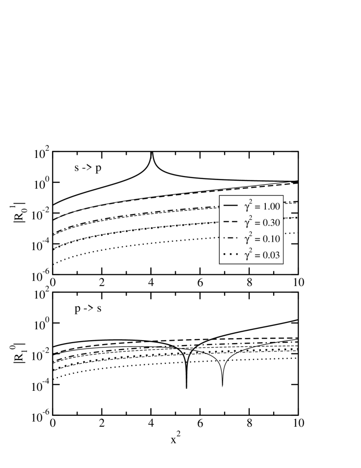
in the neutron+core case for and transitions are derived. They only depend on the value of the radial wave functions and their logarithmic derivative at the radius of the square well. The ratio
| (30) |
as a function of for and transitions, respectively, is displayed in figure 4 for various values of assuming the same depth of the square-well potential for the bound and scattering state. For halo nuclei with small the total radial integral is clearly dominated by the exterior integral even at values . In the case of a resonance in the scattering wave (e.g. for the transition with ) the ratio shows a distinct peak since the scattering wave function penetrates into the core of the nucleus. In the limit one finds the scaling laws
| (31) |
depending on the principal quantum number (see appendix A.4). For larger values of the ratios become smaller but they remain finite for a given in the limit . As can be seen from figure 4 these scaling laws are also well satisfied for larger values of as long as there are no resonances or accidental zeros in the interior integral. For halo nuclei one clearly sees that the total radial integral is well approximated by the exterior part with the asymptotic form of the wave functions that is independent of the details of the potential. This will be even more true for higher multipolarities due to the factor in the radial integral. Only the parameters , , the ANC and the phase shift are really relevant.
2.4 Dipole integrals and commutator relations
In the case of electric dipole transitions the relevant reduced matrix element (2.3) can also be calculated with the help of the commutator relation [39, 40]
| (32) |
Introducing the scaling parameters and , we find
| (33) |
for the dipole matrix element. This equation directly shows the occurence of a pole at , i.e., . This derivation is much more transparent than the corresponding discussion in [41] for radiative capture reactions. For halo systems with small nucleon separation energies one immediately sees that a series expansion of the dipole matrix element (33) in the parameter (or the energy ) is only of limited value because of the small radius of convergence (). It would be more advantageous to expand the matrix element with the double commutator in a power series in .
The double commutator can be calculated assuming different forms of the potential in the Hamiltonian of the system. The simplest case is a central potential that commutes with , i.e. . With the radial integral (25) can be expressed as
| (34) |
In the neutron+core case with a square-well potential
| (35) |
we find that the radial integral is given by
| (36) |
It depends only on the values of the initial and final radial wave function at the radius and the depth of the potential in the dimensionless parameter
| (37) |
that characterizes the strength of the interaction. It is not surprising that this result can also be derived by evaluating the radial integral (25) directly (see appendix A.4). For more realistic potentials the derivative also peaks close to the nuclear radius and the radial integral is mainly sensitive to the bound and scattering wave functions near the nuclear surface.
For finite values of the radial integral (36) shows a dependence for large energies independent of the orbital angular momenta in the initial and final state. (The wave function is independent of and shows an oscillatory behaviour for large .) This dependence is sufficient for the convergence of the non energy-weighted and energy-weighted sum rules as discussed in section 4.
In the proton+core case the potential is well approximated by
| (38) |
and the radial integral becomes
with the integral
| (40) |
that converges much more rapidly than the usual transition integral. This contribution only depends on the parameters , , and . The ratio
| (41) |
of the two contributions in (2.4) is depicted in Fig. 5 as a function of for typical values of and for both and transitions. It is clearly seen that the ratio of the two contributions to the total radial integral increases with increasing and decreasing . This is expected since Coulomb effects become stronger for larger and the bound state wave function at larger radii is less steep for smaller . The ratio (41) decreases for larger values of with a larger effect for large values of . Generally, transitions are more strongly affected by the correction than transitions , however, for large (less halo effect) the difference becomes smaller.
Ususally, one can expect that the Hamiltonian contains more general potentials that do not commute with [42], e.g.,
| (42) |
with a central potential and a spin-orbit contribution . In this case the double commutator in (32) can be calculated explictly and a rather complicated radial integral is obtained. Alternatively, we can introduce and with projection operators and on the final and initial state, respectively. Then the commutator relation (32) can be generalized to
where , and denotes the anticommutator. For the potential (42) we find with and
| (44) |
where , , and are the total angular momentum, the orbital angular momentum, and the spin of the nucleon, respectively. The central potentials with are now different in the bound and scattering states, however, the various contributions in (2.4) can be calculated easily. Assuming a square-well potential for both and with the same radius but different depths the radial integral corresponding to (36) becomes a more complicated expression that contains also derivatives of the wave functions at the radius . Explicit expresssions are obtained from adding the interior and exterior integrals as derived in appendix A.4. Also other forms of the potentials, e.g., a surface-peaked spin-orbit potential , can be considered. However, we omit the details of the calculation.
2.5 Cross sections
The reduced transition probability determines the cross sections for photo-nuclear reactions. The photo dissociation cross section
| (45) |
is proportional to where is the sum of the binding energy of the nucleus with respect to the breakup into and the relative energy in the final state. The photo absorption cross section (45) also enters the cross section for the electromagnetic dissociation reaction during the scattering of an exotic nucleus on a target nucleus . A first-order calculation gives
| (46) |
with virtual photon numbers that can be calculated in the semiclassical theory or in prior-form DWBA in the quantal approach. The factorization of the cross section (46) into contributions that are related to the nuclear structure of the exotic nucleus and to the excitation mechanism is no longer valid if higher-order effects from the target-fragment interactions are significant. From the photo dissociation reaction it is also possible to extract information on the radiative capture reaction that for low energies is relevant for nuclear astrophysics. The capture cross section
| (47) |
is obtained by applying the theorem of detailed balance. The photo absorption cross section (45) is multiplied with a factor that contains the spins of the particles , the photon momentum , and the final state momentum .
For electric dipole transitions it is easy to find the high-energy behaviour of the various cross sections. From equation (34) the dependence of the radial transition integral is extracted. With (2.3) and (2.3) one finds or . This corresponds to a dependence and for the photo dissociation and radiative capture cross sections at high energiess , respectively. We note that in the case of the photodissociation of atoms, with the shape of the Coulomb potential, one finds the same law, see [43].
2.6 Effective-range expansion
The nucleon-core interaction that is responsible for the binding of the system also generates structures in the continuum. At low energies in the continuum the phase shifts are insensitive to the details of the nuclear potential as long as no resonance appears. They are determined by only a few parameters that are given by the effective-range approximation. E.g., in the case of charged-particle scattering the low-energy phase shift in the partial wave with orbital angular momentum is determined by the scattering length and the effective range in the expansion [44]
| (48) |
with the function
that depends on the Sommerfeld parameter in the argument of the Digamma function and is Euler’s constant. The constants for increasing are obtained by means of a recursion relation
| (50) |
Note that and for do not have the dimension of a length. The effective-range expansion can be used to express the phase shifts directly as functions of the momentum .
Taking only the scattering length and the effective range into account one does not necessarily find a good approximation of the phase shift over a wide range of energies in the continuum. However, the effective-range expansion motivates to introduce an energy-dependent function via the equation
| (51) |
with the dimensionless parameter where is constant for a given nucleus. In general, the function depends on the momentum in the final state. It fully describes the effects of the interaction in the scattering state at all energies. The quantity varies slowly with the parameter as long as no resonance is approached. For small one can identify with a reduced scattering length since the usual scattering length is obtained in the limit
| (52) |
and for we obviously have .
3 Reduced radial integrals and shape functions
Considering the asymptotics of the radial wave functions one can define dimensionless reduced radial integrals by the relation
| (53) |
At low energies the main contribution to the radial integral arises from radii larger than the radius of the nucleus. This is especially true for halo nuclei where the probability of finding the nucleon inside the range of the nuclear potential is small (see subsection 2.2). Neglecting contributions from radii smaller than a cutoff radius the reduced radial integrals can be approximated by
| (54) |
where and denote the real and the imaginary part of the function
Here, as in the following, the quantum numbers , , , and have been suppressed if no confusion arises. The nuclear phase shifts encode the effects of the final-state interaction. For one obtains the results without the nuclear interaction between the nucleon and the core. Note that the function depends only on the parameters , and .
If there is only one fixed pair in the initial state and similar in the final state the expression for the reduced transition probability reduces to
with the dimensionless shape function of the transition strength
| (57) |
that completely contains the dependence on the momentum in the continuum. Similarly, one can define the characteristic shape functions for the photo absorption
| (58) |
and for the capture cross section
| (59) |
The expression (3) directly shows the dependence of the transition strength on the characteristic parameters and of the ground state. For small separation energies of the nucleon the strength becomes very large since is a small number. Note that the ANC in general depends on , too. In a model for neutrons in a square-well potential one finds a dependence for and for , respectively, for small (see Appendix A).
When the nucleon is a neutron the reduced radial integrals can be calculated analytically (see Appendix C). Then the functions (54) only depend on the dimensionless variables and and the phase shift in the final state. It is found that the reduced radial integrals have the general form
with polynomials/rational functions . Explicit expressions are given in Appendix C. In general they are complicated functions of and .
From the discussion in subsection 2.4 a dependence of the reduced radial integrals for dipole transitions is expected for large . However, the integrals (3) for show a different high- behaviour and the convergence of the sum rules (see section 4) is not guaranteed. This is a consequence of neglecting the interior contribution to the radial integral that becomes relevant at high relative energies since the nucleon penetrates into the core. Thus, the reduced radial integrals (3) are only a good approximation for not too high relative energies in the continuum. In comparison, equation (36) is valid irrespective of the halo nature of the system and for all energies but only for and the square-well case; it contains all contributions to the radial integral from zero to infinity. Equation (3) is a good approximation for halo nuclei at small relative energies, since the interior contributions are small in this case (cf. Fig. 4). It can also be applied easily to cases where the potential is different in the bound and scattering states. It is worthwhile to study some limiting cases.
3.1 Shape functions in n+core systems without final-state interaction

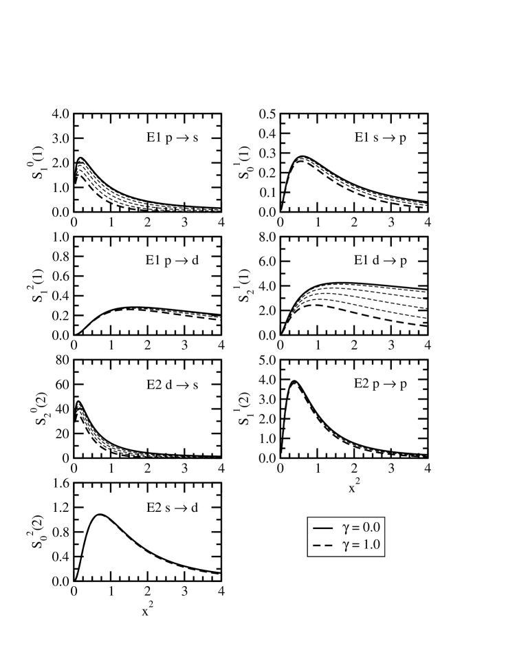
Without nuclear interaction between the neutron and the core in the final state the phase shift is zero and there is no contribution from the integral with the irregular wave function in (54). The contribution for radii in the radial integral is small and it is possible to take the limit keeping the neutron separation energy or equivalently the inverse bound-state decay length constant. In this limit both and approach zero but the ratio , i.e. the relevant variable for the shape of the strength distribution, is independent of . In this case the reduced radial integrals (3) assume a particular simple form. They only depend on this dimensionless variable . From the reduced radial integrals the shape functions (57) of the reduced transition probability are easily derived. The functions in the limit with are given in table 2. Especially the expression is well known, see, e.g., [13, 45]. It can be found in a different notation also in Refs. [2, 37].
In Fig. 6 the generic form of the shape functions is shown as a function of for and transitions from a bound state with orbital angular momentum to a scattering state with orbital angular momentum . The dependence of the transition shape on the centrifugal barrier is clearly seen. The peak at small energies is more pronounced for low orbital angular momenta . Only for and waves in the continuum a large transition strength is found close to the threshold. At low we have the typical dependence
| (61) |
The shape function for photo absorption has the same dependence as for small final state momenta. The shape function for radiative capture , on the other hand, shows a dependence for small momenta in the continuum due to the additional momentum dependent factor from the theorem of detailed balance (47), see equation (58).
In case of a finite cutoff radius in the radial integral (25) the shape function depends on both and . Since is fixed for a given nucleus is it reasonable again to use and as independent parameters. For halo nuclei with small nucleon separation energy will be a small quantity. As long as does not become too large, e.g. for heavy nuclei, will also be small. The variation of the shape functions with gives an estimate of the contribution to the radial integral from the nuclear interior. In Fig. 7 the change of the shape functions with is shown for the transitions of Fig. 6. There is a clear systematic trend. The shape functions are less sensitive to a change in for larger final state orbital angular momentum and higher multipolarity because of the suppression of the integrand at small from the spherical Bessel functions and from the transition operator, respectively. On the other hand, a larger orbital angular momentum in the bound state increases the sensitivity since the wave function introduces a dependence at small radii. This explains the strong -dependence of the shape function .
3.2 Shape functions in n+core systems with final-state interaction
For neutron scattering the finite-range expansion (48) reduces to
| (62) |
since . Taking only the contributions with and into account the phase shift crosses the value at an energy . This behaviour produces a resonance in the corresponding partial wave if the phase shift is increasing that, however, does not have to be physical. In general, the actual energy-dependence of the phase shift close to a resonance at energy is given by the Breit-Wigner form with positive width where the parameters and are not related to and in the effective-range expansion. Particular values for these parameters that correctly reproduce the phase shift at low momenta will not necessarily reproduce the position and the width of an actual resonance with orbital angular momentum . However, the phase shift can be calculated with the help of the relation
| (63) |
for general cases assuming an energy dependence of the function . It replaces the phase shift in order to take the FSI in the scattering wave function into account. The dimensionless function is related by
| (64) |
to the function introduced in Ref. [46] for a low-energy expansion of cross sections for radiative capture reactions.
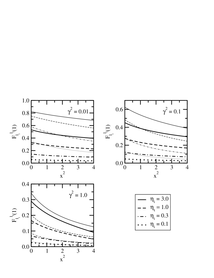
The function is of the order of unless the logarithmic derivative of the scattering wave function at radius is close to , see eq. (121). It is useful in expansions of the shape functions if the limit is considered. On the other hand, the scaled function
| (65) |
(usually of order one) is the appropriate quantity if the limit is studied. In this case we have
| (66) |
with constant radius .
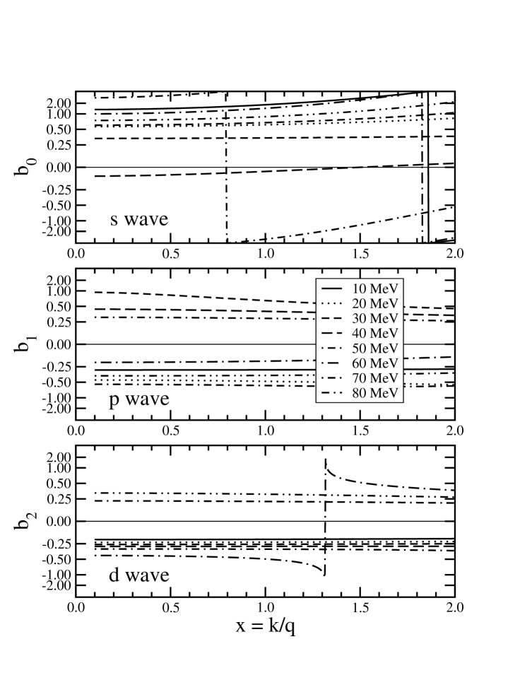
Typical values of and can be estimated from examples employing a single particle model where a nuclear potential of Woods-Saxon form with typical parameters is assumed. In Figure 8 the function for orbital angular momenta is shown as a function of for the scattering of a neutron on 10Be assuming different depths of the potential. In most cases the function is quite constant as a function of except when there is a resonance (vertical lines in Fig. 8) in the continuum for a certain fixed depth . For and waves is usually in the intervall ; for waves covers a larger range. Assuming a zero-range potential for the neutron-core interaction the scattering wave function is given by with the bound state parameter determined by the binding energy. The wave scattering length is just corresponding to and . Since the ground state is close to the threshold for a halo nucleus becomes unnaturally large and there will be a large effect on the continuum in the same partial wave. However, the partial waves in the final state for an electric excitation have a different orbital angular momentum and parity and usually there will be no resonance in the energy range of interest. In general it is reasonable to assume with a weak momentum dependence.
The phase shift in the general expression for the reduced radial integral (3) can be replaced by the function using the explicit relation (63). For some of the transitions it is still possible to take the limit in the reduced radial integrals for . The corresponding shape functions are given in table 3. For the other transitions the reduced radial integral and the shape function diverges. It is obvious that the dependence at small is obtained again but the modulus is modified in the limit as compared to the generic shape functions in table 2 because of the FSI.

In Fig. 9 the dependence of the shape function in the limit on is shown for the cases of table 3. (Transitions with are not relevant.) The function varies in the interval . This corresponds to reasonable values that are far from a resonance in the particular continuum channel. Depending on the magnitude of the shape functions show a pronounced variation around the generic form that reflects the effect of the potential in the final state. Small changes in the reduced scattering length lead to a smaller effect for higher orbital angular momenta due to the dependence in the analytical expressions. For positive values of one finds an increase of whereas a negative leads to a decrease in absolute value. There is also a change in the shape observed and a shift of the maximum. This shift becomes noticable only for large values of . The position of the maximum moves to larger with decreasing for and waves in the final state, whereas the trend is opposite for -wave final states. There is also a clear hierachy observed. The maximum of the shape function appears at higher with larger orbital angular momentum in the continuum.
The analytic expressions of the shape functions in table 3 were obtained by extending the asymptotic form of the bound and scattering wave functions to zero radius in the radial integral. The integrand with the regular scattering wave function shows a dependence; in contrast to that one finds a behaviour at small for the integrand with the irregular scattering wave function. One might expect that the irregular contribution is overestimated in this limit since it diverges for . Expanding the general shape functions in powers of with constant one finds the results as given in table 4. The functions again show the typical dependence at low but the slope depends less strongly on for finite than for the functions given in table 3. The shape functions of the transitions and () for () diverge in the limit or .

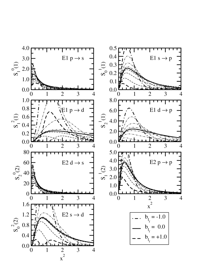
Fig. 10 shows the dependence of the shape functions on for constant , i.e. a constant cutoff radius . This value of corresponds to fm in case of neutron scattering on 10Be with a bound state parameter fm-1 for a neutron separation energy of MeV. The shape functions are very similar to the case with , cf. Fig. 9, except for two cases where diverges in the limit for finite . In general the shape functions for finite are slightly smaller than in the case . Final state effects for a finite value of are less pronounced than in the case with but the differences is small. Therefore the dependence of the shape functions in table 3 on gives a reasonable impression about the importance of the final state interaction. For transitions or a strong dependence of the shape function on is found. The shape and magnitude of the reduced transition probability depends sensitively on the choice of and .
The sensitivity of the shape functions to final-state effects on the neutron separation energy can be estimated from an expansion of in terms of by replacing the function with the quantity as defined in equation (65). This approach was introduced in [25]. Analytical expressions for dipole transitions are given by
| (67) | |||||
| (68) | |||||
| (69) | |||||
| (70) |
These expansions are consistent with the results in table 4 in the limit (, see eq. (65)). There are corrections to the shape functions in table 3 linear in for transitions and proportional to for transitions for finite values of . For and transitions one finds corrections to the forms in table 3 of order and , respectively. They contain a contribution depending on the interaction () and a correction from the finite size of the system. Transitions are affected more strongly by the interaction than transitions .
Another approach to estimate the sensitivity to the FSI is a comparison of the shape functions by scaling and appropriately. In Fig. 10 the shape functions were shown for and constant . Multiplying by a factor of 2 corresponds to an increase of by a factor of 4. In order to cover the same range of scattering lengths as in Fig. 10 also the interval for the function has to be increased to because the ratio has to be kept constant, cf. Eq. (52). The corresponding shape functions for are depicted in Fig. 11. It is obvious that a higher neutron separation energy leads to a much stronger dependence of the shape functions on the strength of the final-state interaction. This behaviour is easily understood from the radial dependence of the bound state wave function. For larger separation energy the slope of the asymptotic wave function is much steeper since increases. The radial integral is more sensitive to a small shift of the continuum wave function from a finite nuclear phase shift because the main contribution to the integrals arises from a smaller intervall in the radius on the surface of the nucleus. The effect is less pronounced for waves in the final state but increases dramatically for higher partial waves in the continuum.
3.3 Shape functions in p+core systems


The Coulomb interaction in p+core systems leads to a systematic modification of the characteristic shape functions as compared to n+core systems. Since analytical results are not available in general one has to resort to a numerical integration of the radial integral (3) if the dependence on arbitrary values of is studied. In Ref. [47] an analytic result for the radial integral was obtained in the special case of scattering on a solid sphere with given radius. For it is possible to obtain analytical results in an approach with an expansion for small energies as presented in Refs. [41, 48]. For small one finds a suppression of the shape function approximately proportional to with the Sommerfeld parameter of the scattering state. This scaling is characteristic for a case with a Coulomb barrier. However, at larger energies the absolute value of the shape functions is determined by the Sommerfeld parameter of the bound state since it defines the range of radii with the largest contribution to the radial integral. In figure 12 the variation of the shape functions with for and for various transitions is shown. The functions are scaled with . Effects from the nuclear interaction in the final state are not taken into account. For the results for neutrons are recovered. With increasing the maximum of the shape function shifts to higher , i.e. to higher relative energies. At the same time the width of the strength distribution increases and the absolute value of reduces considerably (note the scaling).
At low the suppression of the shape functions with finite as compared to the case is quantitatively given by the factor as defined in equation (50). For corresponding to we have . This suggests to scale the shape functions for the proton+core case with the penetrability factor . In figure 13 the ratio
| (71) |
is depicted for various transitions and parameters . The ratio only weakly depends on . Therefore, the main difference between the proton+core and neutron+core cases is well described by the penetrability factor .
There is a major difference between n+core and p+core nuclei. Due to the increasing Coulomb barrier the observation of a large transition strength at low relative energies will be lost for heavier p+core nuclei and the difference between transitions of different orbital angular momenta in the initial and final states will be become smaller. In contrast, even for heavy n+core nuclei the strong transition strength at small energies will persist and the shape will still be characteristic of the particular transition. In principle, variations of the generic shape functions as shown in figure 12 with finite parameters and can be studied along the lines as for the n+core case. Very similar trends are observed and we omit a detailed discussion.
4 Total transition strength and sum rules
The total strength for an transition from a bound state with quantum numbers to all possible final states is related by the non energy-weighted sum rule
to the expectation value of the initial bound state with orbital angular momentum , see, e.g., [49]. Note that for the integration over the energy not only continuum states but also bound states have to be taken into account if they can be reached by an transition from the initial bound state. In the special case of dipole transitions the root-mean-square radius of the bound state wave function determines the total strength. From the scaling laws of as discussed in subsection 2.2 we expect a divergence of the total transition strengths and for and , respectively, in the limit . In contrast, the total strength should remain finite for larger orbital angular momenta of the bound state wave function.
The total reduced transition probability to the continuum is obtained in our approach with asymptotic wave functions from
with the dimensionless integral
| (74) |
Evidently, the continuum contribution is only a fraction of the total strength if the FSI allows the occurrence of bound states in the corresponding channels. Since we use only the exterior contribution to the radial integral it is not guaranteed that the high energy behaviour of the reduced radial integrals (3) is correct. Indeed, generally we do not find the dependence for transitions as expected from the general considerations in section 2.5. For large there is a sizable contribution from the interior integral that is necessary to generate the correct dependence at high energies. However, the main contribution to the integral (74) arises at small close to the threshold and as long as the integral converges it will give a reasonable approximation of the total transition strength.
If one assumes that there is no nucleon-core interaction in the final states (i.e. plane waves) the full strength lies in the continuum. In this case the functions can be calculated analytically for neutron+core systems in our approach. These functions are given in table 5 where we suppressed unimportant quantum numbers for simplification. The integrals and diverge in the limit but remain finite for . In the limit , i.e. if the bound state does not develop a halo, the functions become very small.
The total transition strength (4) is proportional to . The scaling of the ANC in the limit can be obtained by considering the square-well model (see appendix A). We find
| (75) |
for . Taking this dependence into consideration we find the scaling of consistent with the expectation from the non energy-weighted sum rule.
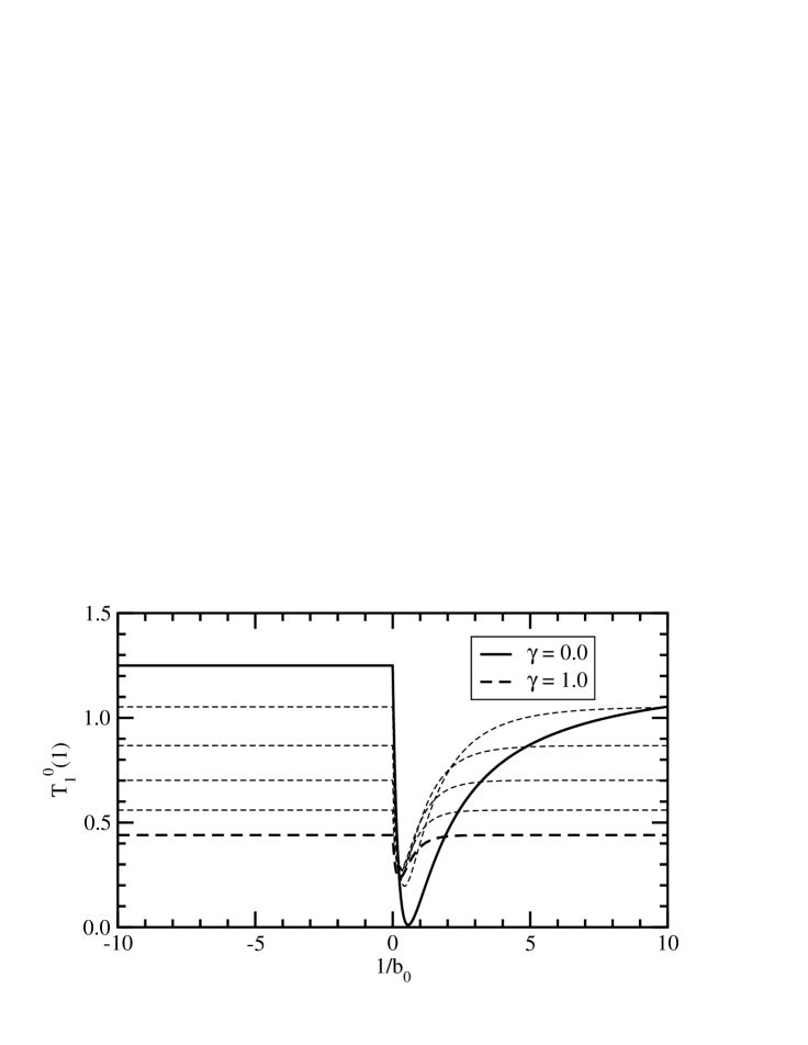
Now, let us consider the case with non-vanishing nuclear interaction in the continuum states. The FSI is parametrized in our approach by the function that in general depends on the energy . If we assume that is constant for all energies the functions can be calculated analytically again. One obtains, e.g. for the transition
| (78) |
For other transitions the expressions become quite complicated and we abstain from giving them here. Since the function cannot be assumed constant over the whole range of continuum energies one cannot expect that the calculated corresponds to a reasonable result in general. However, it is sufficient to assume that the function does not vary too much over the peak of the transition strength that is described by the shape function . For large the excitation spectrum is distorted significantly in the relevant low-energy region.
Equation (78) is quite instructive. It gives a good idea how the strength is modified when the depth of the nuclear potential (with reasonable geometry) changes. For there is a reduction of the total strength in the continuum whereas in the case no reduction is found. This behaviour is related to the occurrence of bound states in the -wave continuum. For the nuclear phase shift and the function is zero. Increasing the potential depth the phase shift at low energies becomes positive, corresponding to a negative scattering length. Increasing the depth further will lead to a more negative and a resonance will appear at low energies. Then there comes the point where the potential will be able to support a bound state and suddenly jumps to a large positive value. Increasing the depth further will reduce the scattering length again. Finally, becomes zero and the cycle starts again. Considering this relation between strength of the potential and the scattering length it is reasonable to plot as a function of as depicted in figure 14. As long as the potential is not able to bind a state the continuum strength does not change. As soon as a resonance in the continuum becomes bound a sudden drop of the transition strength is observed that recovers to its initial value when approaches zero from positive values. An analogous effect was found for the transition for the excitation of 11Be in Ref. [25]. Similar observations are expected for other transitions.
This effect of the FSI has consequences for the extraction of the ANC or the spectroscopic factor for an assumed ground-state single-particle configuration from experimentally obtained total reduced transition probabilities. When the value of from the experiment is compared to the theoretical result assuming a single-particle model with plane waves in the continuum the extracted ANC or spectroscopic factor will be underestimated if the actual nuclear potential supports also bound states. In the latter case, a part of the total transition strength goes to these bound states, even if they cannot be reached by a transition of the halo nucleon because they are occupied by nucleons of the core.
Using the relation
| (79) |
the energy-weighted (or Thomas-Reiche-Kuhn) sum rule
for dipole transitions is obtained. In constrast to the non energy-weighted sum rule (4) it gives a result independent of the orbital angular momentum of the bound state. In principle, the sum contains all bound and unbound states that can be reached from the initial state by an transition. Since the photon energy is the sum rule (4) can be expressed in terms of the total photo absorption cross section (45) as
for the disintegration into core+nucleon. It has the form of a cluster sum rule since we only consider the excitation of the halo nucleon but not of the core [50, 51]. In our approach we can write for the continuum contribution
with the dimensionless integral
If there are bound states in the final channel we expect . Here again, the remarks on the high energy behaviour of the integrand apply as for the functions (74). For the most important transition without interaction in the continuum states we obtain the finite result
| (84) |
where we suppressed irrelevant quantum numbers. Considering the scaling law (75) of the ANC for we find the correct result (4) for the energy-weighted sum rule in the limit . For the ground state with there are two contributions from and in the final state. In this case the integral diverges with but this dependence is compensated by the scaling of the ANC. However, since the radial integrals in the external approximation do not vanish fast enough with increasing , the correct value for the energy-weighted sum rule is not recovered in the limit .
5 Examples for transition strengths of nucleon+core nuclei
Let us now look at some specific examples of exotic nuclei with nucleon+core structure. The dependence of the reduced transition probability and of the cross sections for electromagnetic transitions on the strength of the fragment-fragment interaction in the final state can be studied in the simple but realistic single-particle model of subsection 2.3. For the nuclear potential a Woods-Saxon shape with the representative parameters fm and where fm is assumed. The depth of the potential in the bound state is adjusted to reproduce the experimental neutron and proton separation energies, respectively. In order to simulate a varying interaction strength in the final states the transition strength is studied for the depth of the Woods-Saxon potential in the continuum in the range from 0 to 80 MeV. In Tables 6 and 7 the separation energy , potential radius , potential depth , and orbital angular momentum for the ground state are given for the neutron+core nuclei and proton+core nuclei, respectively. For simplicity, no spin-orbit potential is considered in the calculations. Also the characteristic parameter is given in Tables 6 and 7. Only nuclei with can be considered to be halo nuclei, however, the boundary to nuclei without an extended nucleon distribution is smooth. For p+core nuclei the parameter is given in addition. A larger value indicates a stronger dominance of Coulomb distortions of the strength. In the case of neutron+core nuclei and transition will be considered. In the case of proton+core nuclei we will study especially excitations. For many observables, a square-well model would also be a good approximation, especially for low energy processes where the “shape independence” is valid to a large extent.
5.1 Neutron+core nuclei
| 11Be | 15C | 17O | 23O | 23O | ||
| [MeV] | 0.504 | 1.218 | 4.140 | 2.740 | 2.740 | |
| [fm] | 2.78 | 3.08 | 3.21 | 3.55 | 3.55 | |
| [MeV] | 54.3765 | 48.562 | 55.3726 | 42.416 | 43.1932 | |
| 0 | 0 | 2 | 0 | 2 | ||
| 0.413 | 0.722 | 1.393 | 1.264 | 1.264 |
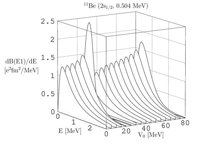
The ground state of 11Be is considered as a neutron in a state coupled to the ground state of 10Be. The experimental neutron separation energy of MeV is quite small so that 11Be is a typical example of a halo nucleus. It was studied by Coulomb dissociation in the experiments [45, 52, 53, 54]. In Fig. 15 the reduced transition probability for a transition into waves is shown for varying depths in the continuum between 0 and 80 MeV in steps of 5 MeV. The E1 strength shows a large peak at relative energies well below 1 MeV typical for a halo nucleus. The shape changes smoothly with increasing potential depth except for close to 30 MeV where a -wave resonance in the continuum becomes bound. For a potential depth similar to the one required for the correct separation energy in the ground state (cf. Tab. 6) the shape of the E1 transition strength is very similar to the result for a plane wave, i.e. MeV. Experimental data for the distribution in 11Be were described in [25] in our approach by fitting the asymptotic normalization coefficient and the constants and in the effective-range expansion for the phase shifts in the waves with total angular momentum and . An unnaturally large value for was found that is related to the low separation energy of the first bound excited state in 11Be. The shape of the dipole strength function in the effective-range approach was found to agree very well to a calculation in the Woods-Saxon model. A corresponding figure and more details can be found in Ref. [25].
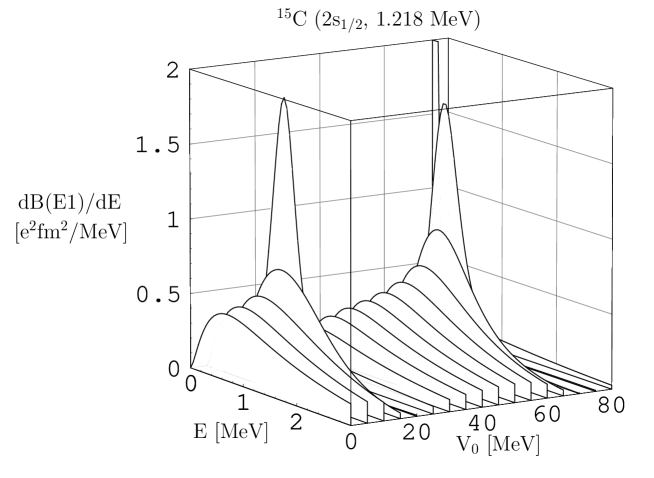
Another example of a neutron+core nucleus with the neutron in a wave ground state is 15C but with a larger neutron separation energy of MeV [55]. Comparing the dependence of the dipole transition strength on the potential depth as shown in Fig. 16 with the case of 11Be one observes a stronger variation of the shape and absolute value. This clearly shows the increased sensitivity of the transition strength on the final-state interaction when the neutron separation energy increases as expected from the analytical model in subsection 3.2. Again, the reduced transition probability changes quite abruptly when a wave resonance in the continuum becomes a bound state.
An even more drastic change of the transition strength is observed in the case of 23O when the neutron is assumed to be in a -wave ground state, see Fig. 17. This nucleus with a neutron separation energy of MeV cannot be considered as a real halo nucleus. Yet, it can be said that there is substantial low-energy strength.
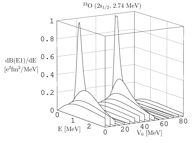
Comparing the three cases 11Be, 15C, and 23O one observes a shift of the peak in the transition strength to higher relative energies in the continuum. The position of the peak scales with the separation energy as expected from the dependence of the shape functions on the ratio in Section 3. Additionally, one finds a reduction of the overall strength as suggested from Eqs. (3) and (4) with an increasing value of the ground state parameter .
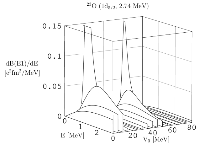
Since the ground state angular momentum of 23O is not known uniquely from experiments [26, 56, 57, 58, 59, 60, 61] it is also possible that the neutron in the ground state occupies a single-particle state. The strength function for an transition to -wave final states under this assumption is shown in Fig. 18. The absolute magnitude is about a factor 4 smaller than in the case of a -wave neutron in the ground state and the maximum is shifted to larger relative energy. This is explained by the additional centrifugal barrier in the wave that reduces the probability of finding the neutron at large distances from the core in the classically forbidden region.
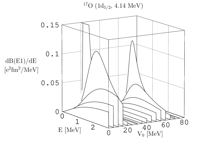
A further example for a neutron+core nucleus with a -wave ground-state configuration is 17O, a nucleus close to the valley of stability. Here the separation energy of MeV is even larger than in the case of 23O and the shape and magnitude of the reduced transition probability to waves in the final state vary drastically with an increasing strength of the final-state interaction.

In Fig. 20 the total transition strength integrated from 0 to 10 MeV is shown for the nuclei discussed above as a function of the potential depth in the continuum. There is a distinctive difference between nuclei with a -wave and -wave neutron in the ground state. In the former case the integrated strength stays almost constant when is increased starting at 0 MeV, i.e. the plane-wave result. Then there is a sudden drop of the total strength when the -wave resonance from the continuum becomes a bound state. However, the total strength recovers to its value for when the potential depth is increased further until the next higher -wave resonance becomes bound. The dependence of the total transition probability on the strength of the FSI is in qualitative agreement with the expectations from the analytical neutron+core model as shown in figure 14. The rise of the total strength after the continuum to bound state crossing is faster when the neutron separation energy is smaller. For halo nuclei there is only a small variation of the total reduced transition probability if one is not too close to a potential strength where the crossing appears. When the neutron is in the -wave ground state there is already a considerable dependence of the total strength on the depth of the potential close to the plane-wave limit. Beyond the sudden drop of the strength at the continuum-to-bound-state crossing the absolute value increases again but it does not reach the plane-wave limit again. Comparing the total strength calculated for a continuum potential that is identical to the bound state potential (filled circle in Fig. 20) one immediately finds that the integrated strength is almost the same as in the plane-wave case for a -wave neutron in the ground state but it is significantly smaller for a -wave neutron.
5.2 Proton+core nuclei
| 8B | 9C | 12N | ||
| [MeV] | 0.1375 | 1.296 | 0.601 | |
| [fm] | 2.50 | 2.60 | 2.86 | |
| [MeV] | 43.183 | 44.4456 | 36.474 | |
| 1 | 1 | 1 | ||
| 0.190 | 0.613 | 0.466 | ||
| 1.595 | 0.655 | 1.171 |
Systems with proton+core structure show similar features as compared to neutron+core systems, however, with modifications due to the appearence of the Coulomb barrier. Since analytical results for the shape functions are not available one has to resort to the numerical calculations, e.g. in the simple single-particle model.
As examples we consider the three unstable nuclei 8B [14, 15, 62, 63, 64, 65, 66], 9C [67, 68, 69] and 12N [70, 71, 72]. Their ground state is well described by a proton in a -wave bound state. The proton wave function is calculated in a single-particle model. The depth of the potentials was adjusted to reproduce the experimental binding energies as in the case of the neutron+core nuclei. The corresponding parameters of the Woods-Saxon potential are given in table 7. As a consequence the ANC of the bound state wave functions is uniquely determined in this model.
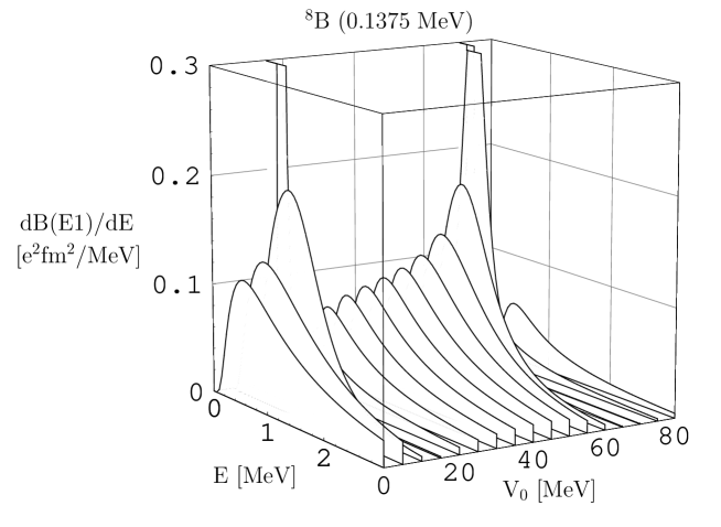
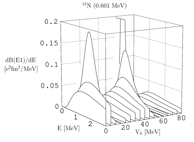
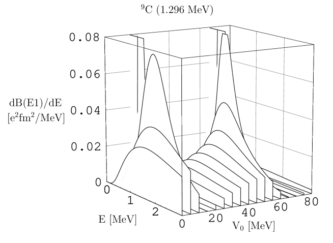
The reduced transition probability as a function of the relative energy is shown in figures 21, 22, and 23 for these nuclei for various depths of the continuum potential. In the calculation it was assumed that the channel spin of the ground state is given by with the core spin . The additional Coulomb interaction between nucleon and core leads to a substantial modification of the shape functions. The transition strength still peaks at low relative energies, however, the maximum is shifted to higher energies as compared to the neutron+core case. For a pure Coulomb wave in the continuum state, i.e. , the maximum is reached at an energy of , and , for 8B, 12N, and 9C, respectively. The larger shift of the maximum to higher energies corresponds to an increase of the parameter , cf. Table 7. In the neutron+core case the maximum is expected at a value of only . The overall shape of the transition strength changes similarly with the depth of the potential as for neutron+core nuclei and the occurence of resonances in the -wave continuum is observed again. Also the integrated reduced transition probability, as depicted in figure 24, resembles in its dependence on the potential depth the results for neutron+core systems between the two cases of and transitions. The value assuming the same potential in the continuum as in the bound state is clearly smaller than the value for pure Coulomb waves in the continuum.

6 Low-energy behaviour and ANC method
At small relative energies the reduced transition probability is strongly suppressed due to penetration effects of the centrifugal barrier. It is useful to change to a different quantity to study the low-energy behaviour and the effects of the nucleon-core interaction in the continuum. Considering the approximation of the shape functions for small in table 4 one can use
| (85) |
with a finite limit for in the case of neutron+core systems. This quantitiy takes the angular momentum barrier into account. Correspondingly the quantities
| (86) |
and
| (87) |
are the relevant forms with a finite value for for photon absorption and radiative capture, respectively, cf. equations (58) and (59). (Note that for the capture reaction the initial and final state are interchanged.) The low-energy behaviour is clearly dominated by the centrifugal barrier in the continuum state. From equation (87) one finds the famous law of the cross section for the neutron capture from a wave in the continuum . The above quantities approach a finite value in the limit that depends on the function . Thus, the interaction in the continuum has an effect on the absolute normalization of the low-energy cross sections.
Apart from the typical dependence the expressions for contain a factor in the denominator that corresponds to a pole at . Considering equation (87) one sees that the shape function for capture reactions has a simple pole at the separation energy . This pole limits the range of convergence of an expansion of the shape functions or cross sections in terms of the parameter or the energy [46]. Since the separation energy is very small for halo systems a corresponding expansion has only limited applicability in this case.
A similar effect is observed for proton+core systems [41, 48]. Here, the low-energy behaviour is dominated by the Coulomb barrier in the continuum state. In nuclear astrophysics one needs, e.g., cross sections for radiative proton capture at very low energies. Instead of extrapolating the strongly energy dependent capture cross section to low energies the astrophysical S factor
| (88) |
is employed. It is weakly dependent on energy and approaches a finite value for . The exponential term depending on the Sommerfeld parameter in the continuum state cancels in leading order the suppression of the capture cross section due to the Coulomb barrier. The factor is proportional to the factor in the theorem of detailed balance (47) from the phase space in the continuum. Considering the scaling of the shape functions for proton+core systems in section 3.3 the generalitzation of (87) is found. The quantity
| (89) |
approaches a finite value for because for with constant . It follows that
| (90) |
for . For small separation energies of the proton in the bound state a strong increase of the S factor at small energies is observed due to the closeness of the pole at . In general, the absolute value of depends on the ANC of the ground state and the scattering length, i.e. the strength of the continuum interaction.
An interesting case is the direct radiative capture from the p + 16O continuum to the first excited () state in 17F that is relevant to nuclear astrophysics [44, 73]. This state with and a small proton separation energy of 105 keV can be considered as a typical halo state. Assuming a radius of fm we find and . At low energies the transition gives the main contribution to the astrophysical S factor (apart from the small contribution of the transition to the ground state with keV). Due to the closeness of the pole at a strong rise of the astrophysical S factor is observed for that is practically independent of the potential in the continuum.

The sensitivity of the low-energy S factor to the interaction in the continuum can be estimated by comparing for various p+core systems as a function of the interaction strength. In figure 25 the dependence of the S factor at zero energy is shown for the reactions (a) 7Be(p,)8B, (b) 11C(p,)12N, and (c) 8B(p,)9C. In all cases we have an transition. The S factor is calculated with varying depths of the Woods-Saxon potential in the continuum waves. Spin-orbit contribution to the potential are neglected for simplicity. For an easier comparision all zero-energy S factors are divided by the zero-energy S factor for pure Coulomb waves, i.e. for the nuclear potential. These are given by (a) eV b, (c) eV b, and (b) eV b in the present model. As is clearly seen in figure 25 the nuclear proton-core interaction directly has an effect on the zero-energy S factor. There is a considerable variation, especially if the depth approaches a value where an -wave continuum state becomes a bound state, e.g. at MeV and MeV in case of the 7Be(p,)8B reaction. Furthermore, we find that the sensitivity to the potential in the continuum state increases with the separation energy of the proton. Assuming the same depth for the continuum potential as for the bound state a S factor is obtained that is somehow smaller, but close the value from a calculation with pure Coulomb waves.
Our results indicate that the zero-energy S factor is not uniquely determined by the ground state ANC that can be extracted from experiments. In general it is necessary to consider the nuclear interaction in the continuum that can be parametrized at small energies by the scattering lengths in the relevant partial waves [46, 48]. One example of particular interest is the 7Be(p,)8B reaction where experimental data from direct and indirect experiments for the S factor have to be extrapolated to zero energy assuming a certain energy dependence from theoretical models [74]. For the 7Be+p system -wave scattering lengths for channel spin S=2 and S=1 (from coupling the spins of the proton and 7Be) have been determined experimentally, however with large uncertainties [75]. More precise values are available for the mirror system 7Li+n [76]. The scattering lengths are easily reproduced in the single-particle model by adjusting the depth of the Woods-Saxon potential in the continuum. As is seen clearly in figure 3 of Ref. [74] the energy dependence of the S factor shows a considerable variation that affects the extrapolation of the experimental data to zero energy.
7 Conclusions and Outlook
In this paper we study single-particle aspects of neutron- and proton-halo nuclei, i.e. the effects which appear when the separation energy of the least-bound nucleon tends to zero. These nuclear systems display universal features, e.g. for the electromagnetic transition strength, that can be described in simple models.
We use different approaches in our theoretical studies: one is a square-well model, for which we obtain remarkably simple analytical results. A more realistic and conventional approach is the model with Woods-Saxon potentials. For our applications to halo nuclei we find that it is, even quantitatively, quite similar to the square-well model. The underlying reason is quite simple: For the low energies relevant for the halo systems there is shape independence: the properties of the potential are encoded in some low-energy parameters which do not depend on the details of the chosen specific potential. Halo nuclei are low-energy phenomena, related to large wavelengths. It is well known that a probe of a given wavelength is insensitive to details of structure at distances much smaller than this wavelength [78]. This means that we can mimic the real short-distance structure (e.g. determined from the nuclear many-body problem or a Woods-Saxon single-particle model) by a simple short distant structure, e.g. a square well model with its agreable analytical properties. The depth and radius parameters serve as adjustable parameters that, e.g., reproduce the binding energy and the scattering length.
We mention also that there is a need to supplement full scale ab-initio microscopic approaches to nuclear structure by some empirical fine tuning of parameters to reproduce the actual position of loosely bound single particle structure, see e.g. [11]. This is indispensible in order to obtain a satisfactory description of low-lying electromagnetic strength.
Following a study of some general single-particle properties we consider the radial matrix elements for electric excitations to the continuum. They essentially depend on the asymptotic wave functions of the bound and scattering states. We identify the important parameters and find rather simple analytical formulae for the most relevant cases for neutron halo nuclei. The most important parameter is depending on the separation energy and the size of the system. It is shown that serves as a convenient expansion parameter. Proton halo nuclei are studied numerically. We find simple scaling laws for the transition strength. We also discuss typical examples for light halo nuclei in the Woods-Saxon model.
We quantitatively analyze the effects of the final-state interaction in the continuum on the transition strength. We find that it is determined mainly by the scattering length. In general, this nucleon-core interaction has an influence on the radiative capture process down to very small energies. This can serve as a warning for the simple application of the ANC method: the results are rather insensitive to the potential in the continuum only for true halo systems.
The power of the present approach is demonstrated by recent applications to actual nuclei [25, 26]. It will serve also as a framework for further applications, notably for the upcoming radioactive beam facilities RIKEN, FAIR/GSI, RIA. One important conclusion is that we quantitatively understand halo effects. It is expected from our studies that neutron-halo effects will show up irrespective of the mass number , whereas proton halo effects will tend to disappear with increasing charge number .
We hope that methods similar to ones developed in this paper will also be useful for the (much) more complicated problems of two-, three, and more nucleon halo nuclei [35, 36]. One early discussion of that problem is [79]. A review on modern approaches in context of effective field theories and references are found in [80].
8 Acknowledgments
We greatfully acknowledge discussions with T. Aumann, U. Datta Pramanik, D. Baye, H. Emling, G. Hansen, and C. Nociforo.
Note added in proof:
In the meantime a paper “Low-lying dipole strength for weakly bound systems: A simple analytic estimate” [81] appeared that contains results which are related to this paper.
Appendix A Neutron in a square-well potential
The problem of a neutron in a square-well potential is well studied for bound and scattering states in the literature, see e.g. [77], and many analytic results have been obtained. However, often only results for a few selected cases are presented. Here, formulas for arbitrary values of the orbital angular momentum are given by generalizing earlier calculations and simplifying the expressions. We also derive results that, to our knowledge, were not quoted in the literature before.
A.1 Wave functions and probabilities
The bound-state wave function
| (91) |
for a neutron with orbital angular momentum and projection in a square-well potential of Radius and depth is completely characterized by the separation energy and the principal quantum number that counts the number of nodes (including the node at ). The radial wave function
| (92) |
is expressed in terms of spherical Bessel and Hankel functions and [38]. The quantities and in the arguments are related by
| (93) |
where an increasing number of radial nodes requires larger values of and of the depth of the potential in the ground state. The relation between and for given is determined by the continuity of the logarithmic derivative
| (94) |
of the radial wave function at . This condition can be written as
| (95) |
with
| (96) |
where
| (97) |
The (complex) constants and are determined by the continuity condition for the wave function
| (98) |
and the normalization condition
| (99) |
with
| (100) |
and
| (101) |
These radial integrals are easily evaluated (see Appendix B) with the results
| (102) |
and
| (103) |
where the continuity equation (98) was used. The quantity
| (104) |
is a rational function in the variable . From the ratio
| (105) |
the probability of finding the neutron at radii
| (106) |
is obtained. In the limit we have
| (107) |
and
| (108) |
independent of the principal quantum number . Equivalent expressions for neutrons were given recently for in Ref. [32].
In case of a scattering state the wave function has the form
| (109) |
for energy with the radial wave function
| (110) |
where
| (111) |
and and are spherical Bessel and Neumann functions, respectively [38]. The phase shift is denoted by and where is the depth of the square-well potential that gives the correct separation energy of the neutron. The continuity condition for the logarithmic derivative
at with
| (113) |
determines the phase shift from
| (114) |
The phase shift is a sum
| (115) |
of the hard-sphere phase shift with
| (116) |
and the additional phase shift with
| (117) |
where
| (118) |
The relation
| (119) |
with the depth of the potential in the scattering state determines the quantity . Generally, in (97) can be different from . In the limit we have
| (120) |
with the scattering length
| (121) |
where
| (122) |
is the scattering length of a hard sphere of radius , i.e. corresponding to .
Defining the penetrability
| (123) |
we can write
| (124) |
with the hard-sphere phase shift . Then the continuity of the wave function at
fixes the constant . The differential probability of finding the neutron inside the square-well potential of radius is given by
Using the continuity relations for the logarithmic derivative one obtains
The probability is determined mainly by the penetrabilities and the differences of the phase shift from the hard-sphere values .
A.2 Root-mean-square radius
The root-mean-square radius of the bound state wave function is obtained from
| (128) |
with
| (129) |
With the help of the integrals in appendix B and the continuity equation for the wave function and the logarithmic derivative we find
Similarly we obtain
The ratio gives
| (132) |
We note
| (133) |
and find
| (134) |
Explicit expressions for are found from the recursion relations (133) with
| (135) |
for . We have
| (136) |
and
| (137) |
for the two lowest orbital angular momenta. This leads to the divergences
| (138) |
in the limit . With the asymptotic behaviour
| (139) |
for we obtain
| (140) |
for higher orbital angular momenta. There is no divergence of the root-mean-square radius in the limit . It approaches a finite value.
A.3 Asymptotic normalization coefficient
The modulus of the quantity is obtained from the normalization condition
| (141) |
It is related via to the ANC . Thus we find for the ANC
| (142) |
In the case one has explicitly
| (143) |
and
| (144) |
For we find
| (145) |
and for
| (146) |
if approaches zero.
A.4 Transition integrals
Using the notation for the radial wave functions of appendix A.1, the interior and exterior contribution to the radial transition integral (25) are given by
| (147) |
and
| (148) |
with the dimensionless integrals
| (149) |
and
| (150) |
These integrals obey the recursion relations
| (151) | |||||
| (152) | |||||
| (153) | |||||
| (154) |
Using the continuity equations (98) and (A.1) we obtain
and the ratio
With the integral formula [38]
| (157) |
for spherical Bessel/Neumann/Hankel functions and we find the monopole functions
| (158) |
and
| (159) |
for general orbital angular momenta . The logarithmic derivative of the scattering wave function is given by
| (160) |
with
| (161) |
We note
| (162) |
similar as in the case for the functions . Introducing and we find
| (163) |
and
The ratio of the monopole integrals is given by
| (165) |
where the relations (97) and (119) were used. If the depths of the potential in the bound and scattering state are identical, i.e. , we have
| (166) |
and the bound and scattering wave functions are orthogonal.
Applying the recursion relations (151) and (153) the relevant integrals for transitions are found to be
and
Then the radial integrals are
and
Similarly, the relevant integrals for transitions
and
are found with the recursion relations (152) and (154). Correspondingly, the radial integrals
and
are obtained.
Assuming that the depths of the potential are the same in the bound and the scattering state, i.e.
| (175) |
we find for the total integrals
| (176) |
and
| (177) |
consistent with the result (36) of the commutator relation. The ratios of the interior to the exterior dipole integral are given by
and
for the transitions and , respectively. The scaling behaviour of these ratios is obtained by an expansion in terms of small with . In the case with a wave bound state we have the relation
| (180) |
Then we find the expansion
| (181) |
with for depending on the principal quantum number . Similarly, for the case of a wave bound state the relation
| (182) |
leads to the expansion
| (183) |
with . Using
| (184) |
we obtain
| (185) |
for small .
Appendix B Integrals of spherical cylinder functions
With the recursion relations [38]
| (186) | |||
| (187) |
for any spherical Bessel, Neumann or Hankel function the well-known integral formula
| (188) |
is easily proven. In a similar fashion the new relation
| (189) |
is obtained. Similarly, integrals with higher powers in can be treated. Introducing the logarithmic derivative
| (190) |
with
| (191) |
one finds
| (192) |
and
With these relations we obtain
| (194) |
and
Appendix C Radial transition integrals for neutron+core systems
In the case when is a neutron analytical expressions of the functions are found. With the Coulomb wave functions
| (196) |
in the integral (3) reduce to spherical Bessel and Neumann functions [38]. Similarly, the Whittaker function
| (197) |
reduces to a spherical Hankel function. This leads to
| (198) |
with the quantities and . From the recursion relation
| (199) |
for any spherical Bessel function the recursion relations
| (200) | |||||
| (201) |
for the functions are obtained that allow the calculation of all relevant functions for increasing values of , , and from basic integrals with . Explicitly one finds
| (202) |
and
with the help of the exponential integral and its recursion relations [38]. Separating real and imaginary parts one obtains the reduced monopole integrals
| (204) | |||||
| (205) |
where the addition theorems of the sine and cosine functions have been used. The reduced integrals for fixed phase shift obey the same recursion relations (200,201) as the functions .
Considering the general form (3) for the reduced radial integrals the monopole functions
| (206) |
and
| (207) |
are extracted from Eqs. (204) and (205). General expression for in Eq. (3) for larger values of , , and can be obtained by applying the recursion relations
Explicitly one finds
| (210) | |||||
| (211) | |||||
| (212) | |||||
| (213) | |||||
| (214) | |||||
| (215) | |||||
| (216) | |||||
| (217) |
for and
| (218) | |||||
| (220) | |||||
| (223) |
for . They cover most of the relevant and transitions between , , and waves in the initial and final states.
References
- [1] G. Baur, C. A. Bertulani, and H. Rebel, Nucl. Phys. A 459 (1986) 188.
- [2] C. A. Bertulani and G. Baur, Phys. Rep. 163 (1988) 299.
- [3] A. Leistenschneider et al., Phys. Rev. Lett. 86 (2001) 5442.
- [4] G. Baur, K. Hencken, and D. Trautmann, Prog. in Part. Nucl. Phys. 51 (2003) 487.
- [5] T. Aumann, in: Proceedings of the International Workshop XXXII on Gross Properties of Nuclei and Nuclear Excitations, edited by M. Buballa, J. Knoll, W. Nörenberg, B.-J. Schäfer and J. Wambach, Hirschegg, Austria, January 11 - 17, 2004, GSI, Darmstadt (2004), p. 243 ff.
- [6] P. G. Hansen and B. Jonson, Europhys. Lett. 4 (1987) 409.
- [7] K. Riisager, A. S. Jensen, P. Møller, Nucl. Phys. A 548 (1992) 393.
- [8] K. Riisager, Rev. Mod. Phys. 66 (1994) 1105.
- [9] P. G. Hansen, A. S. Jensen, and B. Jonson, Annu. Rev. Nucl. Part. Sci. 45 (1995) 591.
- [10] I. Tanihata, J. Phys. G 22 (1996) 157.
- [11] H. Sagawa, T. Suzuki, H. Iwasaki, and M. Ishihara, Phys. Rev. C 63 (2001) 034310.
- [12] Y. Nagai et al., Phys. Rev. C 56 (1997) 3173.
- [13] J. M. Blatt and V. E. Weisskopf, Theoretical Nuclear Physics, Springer-Verlag, New York (1979), p. 48 ff.
- [14] H.M. Xu et al., Phys. Rev. Lett. 73 (1994) 2027.
- [15] L. Trache, F. Carstoiu, C.A. Gagliardi, and R.E. Tribble, Phys. Rev. Lett. 87 (2001) 271102.
- [16] A.M. Mukhamedzhanov, C.A. Gagliardi, and R.E. Tribble, Phys. Rev. C 63 (2001) 024612.
- [17] R. Crespo and F.M. Nunes, Nucl. Phys. A 701 (2002) 637.
- [18] T. Otsuka, M. Ishihara, N. Fukunishi, T. Nakamura, and M. Yokoyama, Phys. Rev. C 49 (1994) R2289.
- [19] A. Mengoni, T. Otsuka, and M. Ishihara, Phys. Rev. C 52 (1995), R2334.
- [20] D. M. Kalassa and G. Baur, J. Phys. G 22 (1996) 115.
- [21] S. Typel and G. Baur, Phys. Rev. C 64 (2001) 024601.
- [22] C. M. Perey and F. G. Perey, Atomic Data and Nuclear Data Tables 17 (1976) 1.
- [23] H. A. Bethe. Phys. Rev. 76 (1949) 38.
- [24] R. G. Newton, Scattering Theory of Waves and Particles, second edition, Springer-Verlag, New York (1982), p. 306 ff.
- [25] S. Typel and G. Baur, Phys. Rev. Lett. 93 (2004) 142502.
- [26] C. Nociforo et al., Electromagnetic excitation of 23O, Phys. Lett. B 605 (2005) 79.
- [27] M. C. Birse, J. A. McGovern, and K. G. Richardson, Phys. Lett. B 464 (1999) 169.
- [28] D. B. Kaplan, M. J. Savage, and M. B. Wise, Phys. Rev. C 59 (1999) 617.
- [29] C. A. Bertulani, H.-W. Hammer, and U. van Kolck, Nucl. Phys. A 712 (2002) 37.
- [30] T. E. O. Ericsson, B. Loiseau, and S. Wycech, hep-ph/0310134 (2003).
- [31] B. R. Holstein, Phys. Rev. D 60 (1999) 114030.
- [32] Z. H. Liu, X. Z. Zhang, and H. Q. Zhang, Phys. Rev. C 68 (2003) 024305.
- [33] I. Hamamoto and X. Z. Zhang, Phys. Rev. C 58 (1998) 3388.
- [34] D. Fedorov, A.S. Jensen, K. Riisager, Phys. Lett. B 312 (1993) 1.
- [35] K. Riisager, D.V. Fedorov, and A.S. Jensen, Europhys. Lett. 49 (2000) 547.
- [36] A. Jensen, K. Riisager, D.V. Fedorov, and E. Garrido, Rev. Mod. Phys. 76 (2004) 215.
- [37] C. A. Bertulani and A. Sustich, Phys. Rev. C 46 (1992) 2340.
- [38] M. Abramowitz and I. S. Stegun, Handbook of Mathematical Functions, Dover Publications, New York (1965).
- [39] P. Ehrenfest, Z. Physik 45 (1927) 455.
- [40] W. Gordon, Ann. Phys. 2 (1929) 1031.
- [41] B. K. Jennings, S. Karataglidis, and T. D. Shoppa, Phys. Rev. C 58 (1998) 3711.
- [42] J.S. Levinger and H.A. Bethe, Phys. Rev. 78 (1950) 115.
- [43] H. A. Bethe and E. E. Salpeter, Quantum Mechanics of One- and Two-Electron Atoms, Plenum, New York (1977).
- [44] C. R. Brune, Nucl. Phys. A 596 (1996) 122.
- [45] T. Nakamura et al., Phys. Lett. B 331 (1994) 296.
- [46] D. Baye, Phys. Rev. C 70 (2004) 015801.
- [47] A. M. Mukhamedzhanov and F. M. Nunes, Nucl. Phys. A 708, (2002) 437.
- [48] D. Baye and E. Brainis, Phys. Rev. C 61 (2000) 025801.
- [49] B. Jonson, Phys. Rep. 389 (2004) 1.
- [50] Y. Alhassid, M. Gai, and G. F. Bertsch, Phys. Rev. Lett. 49 (1982) 1482.
- [51] K. Hencken, G. Baur, and D. Trautmann, Nucl. Phys. A 733 (2004) 200.
- [52] R. Anne et al., Nucl. Phys. A 575 (1994) 125.
- [53] R. Palit et al., Phys. Rev. C 68 (2003) 034318.
- [54] N. Fukuda et al., Phys. Rev. C 70 (2004) 054606.
- [55] U. Datta Pramanik et al., Phys. Lett. B 551 (2003) 67.
- [56] R. Kanungo, I. Tanihata, and A. Ozawa, Phys. Lett. B 512 (2001) 261.
- [57] R. Kanungo et al., Phys. Rev. Lett. 88 (2002) 142502.
- [58] B. A. Brown, P. G. Hansen, and J. A. Tostevin, Phys. Rev. Lett. 90 (2003) 159201.
- [59] M. Thoennessen et al., Phys. Rev. C 68 (2003) 044318.
- [60] E. Sauvan et al., Phys. Rev. C 69 (2004) 044603.
- [61] D. Cortina-Gil et al., Phys. Rev. Lett. 93 (2004) 062501.
- [62] A. Azhari et al, Phys. Rev. C 63 (2001) 055803; Phys. Rev. C 60 (1999) 055803; Phys. Rev. Lett. 82 (1999) 3960.
- [63] K. Ogata et al., Phys. Rev. C 67 (2003) 011602(R), 019902.
- [64] L. Trache et al., Phys. Rev. C 67 (2003) 062801(R).
- [65] A. R. Junghans et al., Phys. Rev. Lett. 88 (2002) 041101; Phys. Rev. C 68 (2003) 065803.
- [66] F. Schümann et al., Phys. Rev. Lett. 90 (2003) 232501.
- [67] D. Beaumel et al., Phys. Lett. B 514 (2001) 226.
- [68] L. Trache et al., Phys. Rev. C 66 (2002) 035801.
- [69] J. Enders et al., Phys. Rev. C 67 (2003) 064301.
- [70] A. Lefebvre et al., Nucl. Phys. A 592 (1995) 69.
- [71] Xiaodong Tang et al., Phys. Rev. C 67 (2003) 015804.
- [72] N.K. Timofeyuk and S.B. Igamov, Nucl. Phys A 713 (2003) 217.
- [73] R. Morlock et al., Phys. Rev. Lett. 79 (1997) 3837.
- [74] B. Davids and S. Typel, Phys. Rev. C 68 (2003) 045802.
- [75] C. Angulo et al., Nucl. Phys. A 716 (2003) 211.
- [76] L. Koester, K. Knopf, and W. Waschkowski, Z. Phys. A 312 (1983) 81.
- [77] A. Messiah, Quantum Mechanics, Vol. I, North Holland, Amsterdam (1961).
- [78] G. P. Lepage, How to Renormalize the Schrödinger Equation, Lectures given at the VIII Jorge Andre Swieca Summer School, Brazil (1997), nucl-th/9706029.
- [79] A. B. Migdal, Sov. J. of Nucl. Phys. 16 (1973) 238.
- [80] E. Braaten and H.-W. Hammer, Universality in Few-body Systems with Large Scattering Length, cond-mat/0410417.
- [81] M. A. Nagarajan, S. M. Lenzi, and A. Vitturi, Eur. Phys. J. A 24 (2005) 63.