Fluctuations in the level density of a Fermi gas

Abstract

We present a theory that accurately describes the counting of excited states of a noninteracting fermionic gas. At high excitation energies the results reproduce Bethe’s theory. At low energies oscillatory corrections to the many–body density of states, related to shell effects, are obtained. The fluctuations depend non-trivially on energy and particle number. Universality and connections with Poisson statistics and random matrix theory are established for regular and chaotic single–particle motion.

The level density is a characteristic property of every many–body quantum mechanical system. Its precise determination is often a key ingredient in the calculation of different processes, like compound nuclear decay rates, yields of evaporation residues to populate exotic nuclei, or thermonuclear rates in astrophysical processes. The first and main step towards the understanding of the density was given by H. Bethe more than sixty years ago. He considered $A$ noninteracting fermions moving in a mean–field potential. By this model he showed that the number of excited states of the many–body (MB) system contained in a small energy window $dQ$ at energy $Q$, $\rho_{\text{\tiny MB}}(A,Q)dQ$, is bethe

$$\rho_{\text{\tiny MB}}(A,Q)=\frac{1}{\sqrt{48}\ Q}\exp\sqrt{\frac{2}{3}\pi^{2}\overline{\rho}\ Q}\ .$$ (1)

Here $\overline{\rho}$ is the average single–particle (SP) density of states at Fermi energy $\epsilon_{\text{\tiny F}}$, and $Q$ is measured with respect to the ground state energy. For a given potential, $\overline{\rho}$ is in general a function of $A$. This expression assumes that the excitation energy is, on the one hand, large compared to the SP mean level spacing $\delta=\overline{\rho}^{-1}$ and, on the other, small compared to $\epsilon_{\text{\tiny F}}$ (degenerate gas approximation). Most of the present knowledge concerning the density of states is based on refinements of Bethe’s result.

In Eq. (1) all the information concerning the SP spectrum is encoded in a unique parameter, $\overline{\rho}$, that describes its average behavior. The exact dependence of $\rho_{\text{\tiny MB}}$ on $A$ and $Q$ is sensitive, however, to the detailed arrangement of the SP energy levels around the Fermi energy. After Bethe’s work, more accurate calculations of $\rho_{\text{\tiny MB}}$ were made bloch . Schematic shell corrections related to a periodic fluctuation of the SP density were computed in ros (see also bm ), introducing the so–called backshifted Bethe formula. Several modifications of Eq.(1) have been done to match the experimental results. These models take into account, for example, shell effects, pairing corrections and residual interactions para , introducing a multitude of coexisting phenomenological parameterizations. The present status of the understanding do not allow to draw a clear theoretical picture of the functional dependence of $\rho_{\text{\tiny MB}}$ with $A$ and $Q$.

Within an independent particle model we demonstrate, through a general theory, the role played by shell effects in the MB density of states. Superimposed to the smooth growth of the density described by Eq.(1), there are oscillatory corrections. To lowest order, these corrections are directly related to energy fluctuations of the system, that may be expressed in terms of sums over the classical periodic orbits. We make a statistical analysis of the density fluctuations, in particular of their probability distribution, typical size, and temperature dependence note . We show that the amplitude of the shell corrections grows linearly at low temperatures, and decays as $T^{-1}$ when $T\gg E_{c}/2\pi^{2}$, where $E_{c}$ is the energy conjugate to the time of flight across the system (temperature is measured in units of Boltzmann constant). The statistical properties of the density fluctuations strongly depend on the regular or chaotic nature of the underlying classical SP motion. Universal properties for each class (regular or chaotic) are found for $T\ll E_{c}/2\pi^{2}$. Besides the fluctuations, we find and discuss corrections to the smooth part of the density in the exponent of Eq.(1). The present analysis considers general properties of fermionic systems. Applications to the specific problem of the nuclear density and to the interpretation of the experimental results will be done in a separate contribution.

The MB density of states is defined as

$$\rho_{\text{\tiny MB}}(A,E)=\sum_{N}\sum_{j}\delta(A-N)\ \delta\left(E-E_{N,j}\right)\ ,$$ (2)

where $E_{N,j}=\sum_{i}n_{j,i}\epsilon_{i}$ is the energy of the $j$-th SP configuration of $N=\sum_{i}n_{j,i}$ particles, $\epsilon_{i}$ the SP energies, and $n_{j,i}=0,1$ are the occupation numbers.

When the SP spectrum consists of equidistant levels separated by $\delta$, e.g. the spectrum of a one dimensional harmonic oscillator, an exact answer to the counting problem exists. The MB excitation energies are integer multiples of $\delta$, each level having a nontrivial degeneracy. It is easy to see that, for a given level defined by an integer, the degeneracy is the same as the number of ways into which the integer can be decomposed as a sum of integers (the partition number). An asymptotic approximation to this well–known mathematical problem was obtained by Hardy and Ramanujan, and later on Rademacher found a convergent series hrr . Expressing it in terms of an expansion in terms of $\overline{\rho}Q$, the result reads

$$\log\left(\rho_{\text{\tiny MB}}^{\text{\tiny HO}}/\overline{\rho}\right)=\sqrt{\frac{2}{3}\pi^{2}\overline{\rho}\ Q}-\log\left(\sqrt{48}\ \overline{\rho}Q\right)-$$ (3)

$$\ \ \frac{\pi^{2}+72}{24\sqrt{6}\pi}(\overline{\rho}Q)^{-\frac{1}{2}}-\left(\frac{3}{4\pi^{2}}-\frac{1}{24}\right)(\overline{\rho}Q)^{-1}+{\cal O}((\overline{\rho}Q)^{-\frac{3}{2}})\ .$$

The first two terms of this expansion reproduce Bethe’s formula.

For an arbitrary SP spectrum the computation of the density of excited states of a fermionic system is a difficult combinatorial problem for which no exact solution is known. We expect, however, that Eq. (3) gives correctly the contribution of the average part of the SP spectrum. What we are seeking here are the variations of the MB density due to fluctuations of the SP spectrum with respect to a perfectly ordered spectrum. A convenient way to express an approximate solution is by means of an inverse Laplace transform of Eq.(2). A saddle point approximation of the resulting integrals yields bm ; fow

$$\rho_{\text{\tiny MB}}(A,E)={\rm e}^{{\cal S}(\mu,T)}/\ 2\pi\sqrt{|{\cal D}(\mu,T)|}\ ,$$ (4)

valid in the degenerate gas approximation. The dependence on $A$ and $E$ in Eq. (4) arises from the saddle point conditions that fix the value of the chemical potential $\mu$ and temperature $T$ of the gas

$${\cal N}(\mu,T)=A\ ,\;\;\;\;\;\;\;\;\;\;\;\;\;\;\;{\cal E}(\mu,T)=E\ .$$ (5)

The functions ${\cal N}=-\partial\Omega/\partial\mu|_{\scriptscriptstyle T}$ and

$${\cal E}(\mu,T)=\Omega(\mu,T)+\mu{\cal N}(\mu,T)+T{\cal S}(\mu,T)$$ (6)

are the particle number and energy functions of the gas, respectively, with the entropy ${\cal S}(\mu,T)=-\partial\Omega/\partial T|_{\mu}$ and the grand potential $\Omega=-T\int d\epsilon\rho(\epsilon)\log\left[1+{\rm e}^{(\mu-\epsilon)/T}\right]$, where $\rho(\epsilon)=\sum_{i}\delta(\epsilon-\epsilon_{i})$ is the SP density of states. In terms of the previous functions, the determinant in Eq.(4) is defined as ${\cal D}(\mu,T)=T^{3}\left[\partial{\cal N}/\partial\mu|_{\scriptscriptstyle T}\ \partial{\cal E}/\partial T|_{\mu}-\partial{\cal N}/\partial T|_{\mu}\ \partial{\cal E}/\partial\mu|_{\scriptscriptstyle T}\right]$. All the necessary quantities involved in the computation of $\rho_{\text{\tiny MB}}$ are therefore defined from $\Omega(\mu,T)$.

The task consists in the evaluation of the entropy and the determinant at values of $\mu$ and $T$ that satisfy the conditions (5). As $A$ and $E$ are varied in Eqs.(5), in general $\mu$ and $T$ do not have a smooth and gentle behavior, because the functions ${\cal N}$ and ${\cal E}$ may have sudden changes due to the discrete nature of the SP spectrum. The difficulty lies in a proper treatment of the smooth part of the variations as well as the fluctuations with respect to it. To this purpose it is convenient to use the semiclassical approximation gutz . The SP density of states is decomposed into the sum of a smooth term ($\overline{\rho}$, given by a Thomas Fermi approximation or Weyl series) plus oscillatory terms $(\widetilde{\rho})$, $\rho=\overline{\rho}+\widetilde{\rho}$. Taking into account only the smooth part of the SP density of states, the calculation of $\rho_{\text{\tiny MB}}$ is relatively straightforward and leads to Bethe’s formula. The oscillatory part depends on the primitive classical periodic orbits $p$ (and their repetitions $r$), $\widetilde{\rho}=2\sum_{p}\sum_{r=1}^{\infty}A_{p,r}\cos\left[rS_{p}/\hbar+\nu_{p,r}\right]$. Each orbit is characterized by its action $S_{p}$, stability amplitude $A_{p,r}$, and Maslov index $\nu_{p,r}$. When inserted into the definition of the grand potential, and after integration with respect to the energy, the fluctuating part of $\Omega$ is given by ruj

$$\widetilde{\Omega}(\mu,T)=2\hbar^{2}\sum_{p}\sum_{r=1}^{\infty}\frac{A_{p,r}~{}\kappa(\frac{r~{}\tau_{p}}{\tau_{\scriptscriptstyle T}})}{r^{2}~{}\tau_{p}^{2}}\cos\left(\frac{\scriptstyle rS_{p}}{\scriptstyle\hbar}+\nu_{p,r}\right).$$ (7)

Here $\tau_{p}$ is the period of the periodic orbit, and $\kappa(x)=x/\sinh(x)$ is a temperature factor that introduces the time scale $\tau_{\scriptscriptstyle T}=\hbar/(\pi T)$ conjugate to the temperature. This expression describes the departures of $\Omega$ with respect to its mean behavior due to the fluctuations of the SP spectrum. By simple derivation of the grand potential the smooth and fluctuating part of all other thermodynamic functions can be obtained. Intensive functions like the chemical potential and the temperature should also be decomposed. We define their smooth parts by the implicit equations

$$\overline{\cal N}(\overline{\mu},\overline{T})=A\ ,\;\;\;\;\;\;\;\;\;\;\;\;\;\;\;\overline{\cal E}(\overline{\mu},\overline{T})=E\ ,$$ (8)

whereas the fluctuating parts are $\widetilde{\mu}=\mu-\overline{\mu}$ and $\widetilde{T}=T-\overline{T}$.

Using Eqs.(5) and the decomposition of the different functions, Eq.(6) may be rewritten as

$$(\overline{T}+\widetilde{T}){\cal S}=E-\overline{\Omega}(\mu,T)-\widetilde{\Omega}(\mu,T)-(\overline{\mu}+\widetilde{\mu})A\ .$$ (9)

If $A$ is large, the smooth part of the grand potential can be expanded in power series of $\widetilde{\mu}$ and $\widetilde{T}$. Keeping terms up to first order, using that in the degenerate gas approximation $\overline{\Omega}(\overline{\mu},\overline{T})\simeq\overline{\Omega}(\overline{\mu},0)-(\pi^{2}/6)\overline{\rho}\ \overline{T}^{2}$, and neglecting variations of $\overline{\rho}$, Eq.(9) becomes

$$(\overline{T}+\widetilde{T}){\cal S} = E-\overline{\Omega}(\overline{\mu},0)+\frac{\pi^{2}}{6}\overline{\rho}\ \overline{T}^{2}+\overline{{\cal S}}(\overline{\mu},\overline{T})\ \widetilde{T}-$$ (10)

$$\widetilde{\Omega}(\mu,T)-\overline{\mu}A\ .$$

This equation is valid for an arbitrary temperature. At zero temperature, the energy of the system is the ground state energy $E_{0}$, and Eq.(10) reduces to

$$0=E_{0}-\overline{\Omega}(\overline{\mu},0)-\widetilde{\Omega}(\mu_{0},0)-\overline{\mu}A\ .$$ (11)

$\overline{\mu}$ remains constant if variations of $\overline{\rho}$ are neglected, but the fluctuating part still depends on temperature. As a consequence the chemical potentials are slightly different. The idea is to subtract Eq.(11) from (10). Before doing that we first need to properly analyze some of the terms. The difference $E-E_{0}=Q$ is the excitation energy of the gas, as well as the term $(\pi^{2}/6)\overline{\rho}\ \overline{T}^{2}=Q$. The latter equation follows from the dependence of the energy on temperature in the degenerate gas approximation, $\overline{\cal E}(\overline{\mu},\overline{T})\simeq\overline{\cal E}(\overline{\mu},0)+(\pi^{2}/6)\overline{\rho}\ \overline{T}^{2}$, and the stationary phase condition (8) for $\overline{\cal E}$ (and the corresponding one at zero temperature). It allows to express the temperature in terms of $Q$. Similarly, $\overline{\mu}$ is obtained by inversion of $\overline{\cal N}(\overline{\mu},\overline{T})$ in (8) which, in the degenerate gas approximation and neglecting variations of $\overline{\rho}$, is independent of $\overline{T}$.

Returning to Eq.(10), the term $\widetilde{T}({\cal S}-\overline{{\cal S}}(\overline{\mu},\overline{T}))=\widetilde{T}\widetilde{{\cal S}}$ is of second order, and is therefore neglected. After subtraction of Eq.(11) and expressing $\overline{T}$ in terms of $Q$, the entropy may be expressed as

$${\cal S}(A,Q) = \sqrt{\frac{2}{3}\pi^{2}\overline{\rho}\ Q}+\frac{1}{\overline{T}}\left[\widetilde{\Omega}(\overline{\mu},0)-\widetilde{\Omega}(\overline{\mu},\overline{T})\right]$$ (12)

$$\approx \sqrt{\frac{2}{3}\pi^{2}\overline{\rho}\ \left[Q+\widetilde{\Omega}(\overline{\mu},0)-\widetilde{\Omega}(\overline{\mu},\overline{T})\right]}\ ,$$ (13)

where, to lowest order, $\widetilde{\Omega}$ has been evaluated at $(\overline{\mu},\overline{T})$ (a similar though improved accuracy is obtained using $\mu$ and $T$, cf. Eq.(15) below). Equation (13) is valid if $\widetilde{\Omega}(\overline{\mu},0)-\widetilde{\Omega}(\overline{\mu},\overline{T})\ll Q$, and puts the result under the form of a backshifted Bethe formula.

A more physical interpretation of Eqs.(12) and (13), that expresses the result in an entirely microcanonical language, is provided by the following connection. It has been shown previously lm3 ; sev that, to leading order in an expansion in terms of $\widetilde{\mu}$, $\widetilde{\Omega}(\overline{\mu},\overline{T})=\widetilde{\cal E}(A,Q)$, where $\widetilde{\cal E}(A,Q)$ are the (shell) fluctuations of the energy of the gas at a fixed number of particles and excitation energy. The shell corrections of Eq.(13) are therefore directly related to the fluctuations of the energy of the system.

A similar analysis can be performed for the determinant ${\cal D}(\mu,T)$ in Eq.(4). To leading order we find

$${\cal D}=\frac{\pi^{2}}{3}\overline{\rho}^{2}\ \overline{T}^{4}=\frac{12}{\pi^{2}}\ Q^{2}\ ,$$ (14)

recovering the same form obtained by Bethe ($2\pi\sqrt{{\cal D}}=\sqrt{48}\ Q$, see Eq.(1)). There exist oscillatory corrections to ${\cal D}$, but these are exponentially small compared to those associated with Eq.(12), and we neglect them.

Equation (12) is the central result of the paper. It expresses, together with Eq.(14), the MB density of states in terms of the particle number $A$ and excitation energy $Q$. It decomposes ${\cal S}$ into a smooth and a fluctuating part, ${\cal S}=\overline{{\cal S}}+\widetilde{{\cal S}}$. The smooth part is given by the usual Bethe’s result (corrections to it may be obtained by keeping higher order terms in $\widetilde{\mu}$ and $\widetilde{T}$ in the expansion). The novelty in Eq.(12) is the additional contribution of oscillatory corrections, $\widetilde{{\cal S}}=[\widetilde{\Omega}(\overline{\mu},0)-\widetilde{\Omega}(\overline{\mu},\overline{T})]/\overline{T}$. They describe shell corrections to the MB density. $\widetilde{\Omega}$ depends on temperature only through the function $\kappa$. The effect of this function is to exponentially suppress the contribution of periodic orbits whose period $\tau_{p}\gg\tau_{\scriptscriptstyle T}$ ruj ; lm3 . Since there is no suppression at $T=0$ (because $\tau_{\scriptscriptstyle T}\rightarrow\infty$), only orbits whose period $\tau_{p}\gtrsim\tau_{\scriptscriptstyle T}$ contribute to the difference $\widetilde{\Omega}(\overline{\mu},0)-\widetilde{\Omega}(\overline{\mu},\overline{T})$. At temperatures such that $\tau_{\scriptscriptstyle T}\ll\tau_{\text{min}}$, where $\tau_{\text{min}}$ is the period of the shortest periodic orbit of the system, the term $\widetilde{\Omega}(\overline{\mu},\overline{T})$ becomes exponentially small, and only $\widetilde{\Omega}(\overline{\mu},0)$ remains. The shell correction $\widetilde{{\cal S}}$ therefore decays as $\overline{T}^{-1}$. This decay contrasts with the more common exponential damping observed in other thermodynamic quantities lm3 .

The behavior of $\widetilde{\Omega}$ (and therefore of $\widetilde{{\cal S}}$) strongly depends on whether $\mu$ or $T$ are varied. As discussed above, a temperature variation modifies the prefactors of the summands in $\widetilde{\Omega}$ (through the function $\kappa$), and therefore produces gentle variations of $\widetilde{{\cal S}}$. In contrast, $A_{p,r}$, $\tau_{p}$ and $S_{p}$ depend on $\mu$. For large values of $\mu$, $S_{p}\gg\hbar$ and the dominant variation with the particle number (or any other parameter that modifies the actions) comes from the argument of the cosine function in $\widetilde{\Omega}$. Rapid oscillations of $\widetilde{{\cal S}}$ are therefore generically expected when the number of particles is varied.

A clearer picture of how the fluctuations behave may be obtained through a statistical analysis. There are two relevant SP scales in the analysis, the mean spacing $\delta$ and the energy conjugate to the shortest periodic orbit, $E_{c}=h/\tau_{\text{min}}$. The ratio $g=E_{c}/\delta$ is typically much larger than $1$ (for instance, $g\sim A^{2/3}$ in a three dimensional cavity). The most simple property of the fluctuations is $\langle\widetilde{{\cal S}}\rangle=0$, where the brackets denote an average over a suitable chemical potential window. This result is valid only to first order in the expansion; it can be shown that higher order terms contribute to a non–zero average. The next non–trivial statistical property is the variance $\langle\widetilde{{\cal S}}^{2}\rangle$, that may be computed using Eq.(7). The result is $\langle\widetilde{{\cal S}}^{2}\rangle=(1/2)\int_{0}^{\infty}dx\ K(x,x_{\text{H}})\left[1-\kappa(x)\right]^{2}/x^{4}$, where $K(x,x_{\text{H}})$ is the rescaled form factor of the SP spectrum (cf Eq.(36) in Ref.lm3 ). The latter function depends on the rescaled Heisenberg time $x_{\text{H}}=h\overline{\rho}/\tau_{\scriptscriptstyle T}$. It describes system–dependent features for $x$ of the order of $x_{\text{min}}=\tau_{\text{min}}/\tau_{\scriptscriptstyle T}$, while it is believed to be universal for $x\gg x_{\text{min}}$. The universality class depends on the regular or chaotic nature of the dynamics, and on its symmetry properties. Taking into account the basic properties of $K(x,x_{\text{H}})$, in chaotic systems we find three different regimes for $\langle\widetilde{{\cal S}}^{2}\rangle$ as a function of $\overline{T}$:

(i) Low temperatures $2\pi^{2}\overline{T}\ll\delta$. In this regime $\langle\widetilde{{\cal S}}^{2}\rangle=c_{4}\pi^{2}\overline{T}/\delta$, where $c_{4}=0.0609...$.

(ii) Intermediate temperatures $\delta\ll 2\pi^{2}\overline{T}\ll E_{c}$. In this regime the size of the fluctuations saturate at a universal constant $\langle\widetilde{{\cal S}}^{2}\rangle=c_{3}/\beta$, where $c_{3}=0.1023\ldots$ and $\beta=1(2)$ for systems with (without) time–reversal invariance.

(iii) High temperatures $2\pi^{2}\overline{T}\gg E_{c}$. The size of the fluctuations decreases with excitation energy, $\langle\widetilde{{\cal S}}^{2}\rangle=\langle\widetilde{\Omega}^{2}(\overline{\mu},0)\rangle[1-8\ {\rm e}^{-2\pi^{2}\overline{T}/E_{c}}]/\overline{T}^{2}$. After an exponential transient, a power–law decay $\langle\widetilde{{\cal S}}^{2}\rangle^{1/2}\propto\overline{T}^{-1}$ is obtained.

The situation is different in integrable systems, where only two regimes are found. At low temperatures the result is identical to that of chaotic systems. The difference is that now the growth extends up to much higher temperatures, $2\pi^{2}\overline{T}\approx E_{c}$, without saturation. At that temperature the variance of the fluctuations is of order $g$. In integrable systems, the maximum amplitude of the fluctuations is therefore reached at $2\pi^{2}\overline{T}\approx E_{c}$, and its typical size is much larger than in chaotic systems. At high temperatures $2\pi^{2}\overline{T}\gg E_{c}$ the decay is almost identical to that of chaotic systems (the coefficient 8 is replaced by a 12).

As shown elsewhere lm3 , $\widetilde{\Omega}(\overline{\mu},\overline{T})$ is dominated, at any $\overline{T}$, by the shortest classical periodic orbits. In contrast, the difference $\widetilde{\Omega}(\overline{\mu},0)-\widetilde{\Omega}(\overline{\mu},\overline{T})$ depends on orbits whose period $\tau_{p}\stackrel{{\scriptstyle>}}{{\scriptstyle\sim}}\tau_{\scriptscriptstyle T}$. For temperatures $2\pi^{2}\overline{T}\ll E_{c}$ the statistical properties of these orbits are universal, and correspondingly the probability distribution function of $\widetilde{{\cal S}}$ is expected to be universal, in the sense that at a given temperature it should only depend on the nature of the underlying classical dynamics (regular or chaotic), and the symmetries of the system. This statement is supported by the fact that in the limit $\overline{T}\rightarrow 0$, $\widetilde{{\cal S}}\approx-\partial\widetilde{\Omega}(\overline{\mu},\overline{T})/\partial\overline{T}$. The probability distribution of the latter quantity was studied in Ref.lm3 ; it was shown that it coincides at low temperatures with that obtained from a Poisson spectrum for integrable systems and from a random matrix spectrum for chaotic ones. As the temperature is raised, the universality of the probability distribution of $\widetilde{{\cal S}}$ will be lost for temperatures of the order or greater than $E_{c}$, where system specific features are revealed.

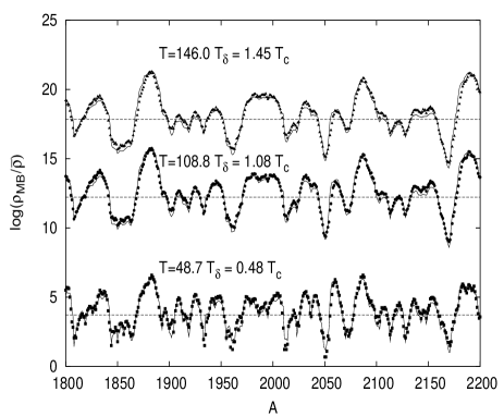
Figure 1: The logarithm of the many-body density of states of $A$ noninteracting fermions in a rectangular billiard of sides $a=\sqrt{(1+\sqrt{5})/2}$ and $b=a^{-1}$. Dots: numerical computation at three different excitation energies; solid curves: theoretical prediction (15); dashed curves: smooth part Eq.(3).

We have checked some of our predictions by a direct numerical counting of the MB density of states in a particular system. Figure 1 shows the results obtained for a gas of about 2000 fermions contained in a two–dimensional rectangular cavity, an integrable system. For each number of particles we compute the MB density of states at three different temperatures, measured in units of $T_{\delta}=\delta/2\pi^{2}$ and $T_{c}=E_{c}/2\pi^{2}$. The theoretical curve is computed according to the expression

$$\log(\rho_{\text{\tiny MB}}/\overline{\rho})=\log(\rho_{\text{\tiny MB}}^{\text{\tiny HO}}/\overline{\rho})+[\widetilde{\Omega}(\mu,0)-\widetilde{\Omega}(\mu,\overline{T})]/\overline{T}\ ,$$ (15)

where $\widetilde{\Omega}$ is given by the periodic orbits of the rectangle. Though the results are similar, $\mu$ instead of $\overline{\mu}$ is used to obtained a more accurate description of the numerical data. A systematic deviation is observed between theory and numerics if the corrections arising from the exact expression Eq.(3) are not included. Notice the extremely good accuracy of this equation, either for the average value of the density as well as for the fluctuations.

The Laboratoire de Physique Théorique et Modèles Statistiques is an Unité de recherche de l’Université Paris XI associée au CNRS.

References

- (1) H. A. Bethe, Phys. Rev. 50 (1936) 332.
- (2) C. Bloch, Phys. Rev. 93 (1954) 1094.
- (3) N. Rosenzweig, Phys. Rev. 108 (1957) 817.
- (4) A. Bohr and B. R. Mottelson, Nuclear Structure, Vol.I, Benjamin, Reading, Massachusetts, 1969.
- (5) A. Gilbert and A. G. W. Cameron, Can. J. Phys. 43 (1965) 1446; A. V. Ignatyuk, G. N. Smirenkin, and A. S. Tishin, Sov. J. Nucl. Phys. 21 (1975) 255; K. Kataria, V. S. Ramamurthy, and S. S. Kapoor, Phys. Rev. C 18 (1978) 549; Y. Alhassid, G. F. Bertsch, and L. Fang, Phys. Rev. C 68 (2003) 044322.
- (6) All over the text, we may either refer to the excitation energy of the system or to its temperature .
- (7) G. H. Hardy and S. Ramanujan, Proc. London Math. Soc. 17 (1918) 75; H. Rademacher, Proc. London Math. Soc. 43 (1937) 241.
- (8) R. H. Fowler, Statistical Mechanics, Macmillan Company, New York, 1936.
- (9) M. C. Gutzwiller, J. Math. Phys. 10 (1969) 1004; R. Balian and C. Bloch, Ann. Phys. (N.Y.) 69 (1972) 76.
- (10) K. Richter, D. Ullmo and R. Jalabert, Phys. Rep. 276 (1996) 1.
- (11) P. Leboeuf and A. G. Monastra, Ann. Phys. 297 (2002) 127.
- (12) P. Leboeuf, Regularity and chaos in the nuclear masses, Lectures delivered at the VIII Hispalensis International Summer School, Sevilla, Spain, June 2003 (to appear in Lecture Notes in Physics, Springer–Verlag, Eds. J. M. Arias and M. Lozano); nucl-th/0406064.