Improved radiative corrections for $(e,e^{\prime}p)$ experiments: Beyond the peaking approximation and implications of the soft-photon approximation

Abstract

Analyzing $(e,e^{\prime}p)$ experimental data involves corrections for radiative effects which change the interaction kinematics and which have to be carefully considered in order to obtain the desired accuracy. Missing momentum and energy due to bremsstrahlung have so far often been incorporated into the simulations and the experimental analyses using the peaking approximation. It assumes that all bremsstrahlung is emitted in the direction of the radiating particle. In this article we introduce a full angular Monte Carlo simulation method which overcomes this approximation. As a test, the angular distribution of the bremsstrahlung photons is reconstructed from H$(e,e^{\prime}p)$ data. Its width is found to be underestimated by the peaking approximation and described much better by the approach developed in this work. The impact of the soft-photon approximation on the photon angular distribution is found to be minor as compared to the impact of the peaking approximation.

1 Introduction

Much of our knowledge about nuclear structure, e.g. the momentum distribution of nucleons in the nucleus, is based on $(e,e^{\prime}p)$ experiments. Currently several such experiments are carried out at the Thomas Jefferson National Accelerator Facility (TJNAF) in Newport News and at the Mainz Microtron (MAMI) in Mainz, taking data at high initial momenta and removal energies in particular. These experiments are aiming at a deeper understanding e.g. of short-range correlations in nuclei and their results are used to check important ingredients of modern many-body theories.

In $(e,e^{\prime}p)$ experiments all particles involved are subject to the emission of bremsstrahlung. On the one hand, consideration of bremsstrahlung contributions is necessary to renormalise the higher-order QED amplitudes. In the second order, divergences from the bremsstrahlung diagrams cancel with those resulting from vertex corrections as has already been shown by Schwinger in 1949 schwinger for electrons scattering off an external potential and for electron-proton scattering by Tsai in 1961 tsai , including divergent contributions from the two-photon exchange (TPE) diagrams. On the other hand bremsstrahlung modifies the cross section integrated over finite intervals of energy loss. Bremsstrahlung photons can be so energetic that they influence the electron’s and the proton’s three-momenta considerably; thereby also the momentum transfer between the two particles is changed. This phenomenon has been studied in a number of papers schiff ; yennie ; maximonisabelle0 ; maximonisabelle1 ; maximon ; motsai ; borie ; borie2 ; friedrich ; calan ; aki1 ; florizone ; maximontjon ; afanasev1 ; afanasev2 ; makins ; afanasev3 both for inclusive and exclusive electron scattering experiments.

Radiative corrections to $(e,e^{\prime}p)$ scattering, including bremsstrahlung, vertex corrections, and vacuum polarization (see Feynman diagrams in fig. 1) can in principle be calculated exactly in (pure) QED and to a good accuracy also including hadronic loops. But for practical purposes several approximations are usually employed when correcting experimental data for radiative effects simc .

One of them is the soft-photon approximation (SPA). It makes use of the fact that in the limit where $\omega^{0}\rightarrow 0$ a bremsstrahlung photon with energy $\omega^{0}$ has neither a kinematic effect on the scattering process nor an effect on the QED propagators and amplitudes. Then the SPA cross section factorizes into the elastic first-order Born cross section times the probability for emitting a bremsstrahlung photon with vanishing energy. Analysis procedures for $(e,e^{\prime}p)$ experiments make use of the SPA simc because it simplifies the calculation of multi-photon bremsstrahlung considerably makins .

Multi-photon bremsstrahlung has to be included into electron scattering data analysis makins ; gupta in order to both impose the physical asymptotic behaviour on the cross section and to achieve percent level accuracy. While these higher-order bremsstrahlung contributions are, in principle, also computable exactly in QED, their evaluation has to be truncated for practical purposes. The SPA is convenient, because it allows for straight-forward inclusion of multi-photon bremsstrahlung into data analysis to all orders makins , as we will see in sect. 2.

The SPA is only valid in the limit of vanishing bremsstrahlung photon energy; however in radiative correction procedures the SPA is applied to photons with energies of up to several hundred MeV. The question arises up to which photon energies the SPA can be considered a good approximation. This paper will not answer that question albeit we will present indications that one of the physical observables (the missing energy) does exhibit sensitivity to shortcomings of the SPA.

$(e,e^{\prime}p)$ data analyses do not employ the ’pure’ SPA (called pSPA in the remainder of this paper) described above. Usually the SPA is modified such that it (i) takes into account kinematic effects due to emission of finite energy bremsstrahlung photons; and it (ii) evaluates the form factors at a modified value of the momentum transfer of the virtual exchanged photon, $q$. We will refer to this ’modified’ SPA as the mSPA. In mSPA each particle emitting bremsstrahlung is put onto the mass shell.

The SPA neglects the proton structure at the bremsstrahlung vertex. But, as has been shown in ref. maximontjon , for the kinematic settings considered in the present manuscript, the influence of the proton structure at the bremsstrahlung vertex is not important.

The other approximation used in radiative correction procedures is the peaking approximation (PA). Most of the bremsstrahlung photons from the electron are emitted either in the direction of the incoming ($e$) or outgoing electron ($e^{\prime}$) and one can observe two radiation peaks at the respective angles. The proton ($p^{\prime}$) bremsstrahlung is much less peaked. At very high momentum transfers one can see a bump (rather than a peak) in its direction, too (see fig. 2). The PA, first proposed for $(e,e^{\prime})$ experiments by L. I. Schiff schiff in 1952, makes use of this observation by assuming that all radiation goes either in the direction of the incoming electron, or the scattered electron. With the advent of coincidence experiments the PA was extended to $(e,e^{\prime}p)$ data makins , assuming that the proton bremsstrahlung was peaked, too. The PA projects the non-peaked contributions to the bremsstrahlung photon angular distribution onto the three peaks. Especially between the two radiation peaks due to electron bremsstrahlung the discrepancy with data becomes large (see fig. 3), limiting the accuracy of $(e,e^{\prime}p)$ data analyses maximonisabelle0 ; maximonisabelle1 .

The purpose of this paper is to remove the PA from $(e,e^{\prime}p)$ data analyses. The need for the removal of the PA became evident when looking at the bremsstrahlung photon angular distribution in H$(e,e^{\prime}p)$ experiments (see fig. 3). In this paper, we introduce a full angular Monte Carlo (FAMC) method which generates multi-photon bremsstrahlung events according to the mSPA photon angular distribution. A similar FAMC code for $(e,e^{\prime}p)$ experiments has been described in ref. afanasev3 . But it has not been inserted into any data analysis codes nor does it handle multi-photon bremsstrahlung. In connection with virtual Compton scattering ref. junior introduces a numerical calculation of radiative corrections beyond the PA, but it considers single-photon emission only, whereas multi-photon contributions are large. To check our results against experimental data we use the simc analysis code simc for Hall C at TJNAF and E97-006 experimental data daniela .

While we do not want to anticipate the results from sec. 5 at this stage we do state here on a preliminary basis that removing the PA can only be a first step on the way to an improved calculation not relying on the SPA. For beam energies envisaged for the TJNAF upgrade, a calculation going beyond the SPA might become necessary, albeit an exact multi-photon bremsstrahlung calculation is impracticable.

This paper is organized as follows: In sect. 2 we introduce the bremsstrahlung cross section including multi-photon bremsstrahlung, discussing the QED divergences. Our calculation partially follows ref. makins , as the resulting equations form the basis for our FAMC calculation. In sect. 3 we extend this approach to a FAMC simulation allowing for any number of bremsstrahlung photons emitted into the full solid angle according to the full angular distribution. In sect. 4 we compare the results of the FAMC

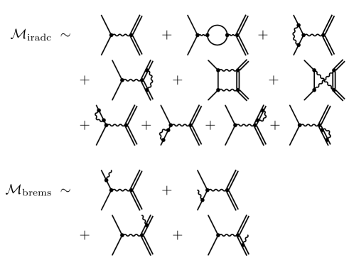
Figure 1: The Feynman diagrams contributing to the internal radiative corrections together with the Born amplitude (top) and the diagrams contributing to the bremsstrahlung amplitude (below). The label ’iradc’ is short hand for internal radiative corrections and ’brems’ stands for bremsstrahlung.

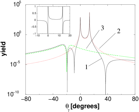
Figure 2: Single-photon angular distribution of bremsstrahlung using the SPA. The full line (1) (black) shows the full angular distribution $A({\Omega_{\gamma}})$ from eq. (4), the dotted line (2) (red) considers pure electron contributions ($ee$) only, the dashed line (3) (green) shows the pure proton contribution ($pp$). The interference term is partially negative and is shown in the inset graph. It is small compared to the other contributions. The momentum transfer is $Q^{2}=15\,{\rm GeV}^{2}$, the entire kinematic setting can be found in table 1. The dip for the proton is due to the fact that a massive particle cannot radiate a photon in forward direction. The same is true for electrons but the width of the respective dip is extremely narrow makins ; junior .

$Q^{2}$	$15\,{\rm GeV}^{2}$
$k^{0}$	$21.00\,{\rm GeV}$
$|{\bf k^{\prime}}|$	$13.00\,{\rm GeV}$
$|{\bf p^{\prime}}|$	$8.882\,{\rm GeV}$
$\theta_{\rm e}$	$13.5^{o}$
$\theta_{\rm p}$	$-19.9^{o}$

Table 1: The kinematic setting used in fig. 2.

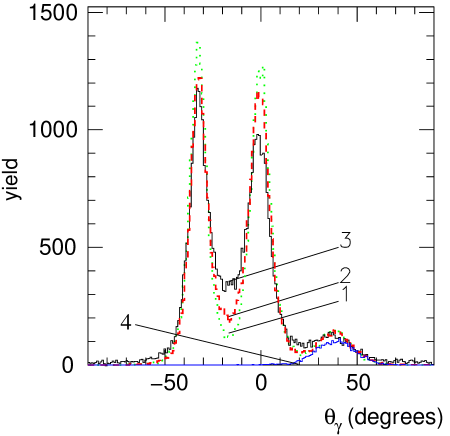
Figure 3: Bremsstrahlung angular distribution for the H$(e,e^{\prime}p)$ reaction at the kinematics given in table 2. The solid curve (3) (black) shows the measured experimental angular distribution of bremsstrahlung. The experimental photon angle $\theta_{\gamma}$ is reconstructed from the missing momentum according to eq. (22). The dotted line (1) (green) and the dashed line (2) (red) correspond to a Monte Carlo simulation based on the PA and take into account detector resolution. The red line takes into account the emission of bremsstrahlung from $e$, $e^{\prime}$, and $p^{\prime}$, whereas the green line only allows for bremsstrahlung emitted solely from either $e$, $e^{\prime}$, or $p^{\prime}$. The solid line (4) (blue) in the vicinity of the proton direction simulates a deficiency of the apparatus (proton punch-through effects). The PA overestimates the two photon peaks in the two electron directions ($e$ and $e^{\prime}$) and it underestimates the bremsstrahlung between these two peaks as well as between the peaks in incident electron direction $e$ and in proton direction $p^{\prime}$ and the radiation on the large-angle tail of the $e^{\prime}$-peak. Both data and simulations account for luminosities and detector efficiencies, and no arbitrary normalization factor is needed.

$Q^{2}$	$2\,{\rm GeV}^{2}$
$k^{0}$	$3.120\,{\rm GeV}$
$|{\bf k^{\prime}}|$	$2.050\,{\rm GeV}$
$|{\bf p^{\prime}}|$	$1.700\,{\rm GeV}$
$\theta_{\rm e}$	$32.5^{o}$
$\theta_{\rm p}$	$-38.5^{o}$

Table 2: The kinematic setting at which the standard radiative corrections and the FAMC simulation are compared to data.

simulation to the PA using the simc code, and in sect. 5 we discuss scope and validity of the SPA, comparing it to the exact QED calculation for single-photon bremsstrahlung from the electron (which will be called ’$1\gamma$ calculation’).

The speed of light has been set to $c=1$ throughout the paper.

2 Bremsstrahlung cross section

In order to obtain the electron-proton cross section to order $\alpha^{2}$ including bremsstrahlung with energy less than $\omega_{\rm max}$,

$$\frac{d\sigma}{d\Omega_{\rm e}}(\omega^{0}<\omega_{\rm max})\,,$$ (1)

where $\omega^{0}$ is the bremsstrahlung photon energy, the amplitudes depicted in fig. 1 are considered. The four bremsstrahlung diagrams contributing to ${\cal M}_{\rm brems}$ are divergent in the limit of vanishing bremsstrahlung photon energy $\omega^{0}$. These divergences cancel the ones both from the TPE diagrams and the vertex corrections schwinger . The TPE diagrams are special cases. While consideration of their divergent pieces is necessary in order to remove all divergences from the scattering amplitudes, their finite contributions are known to be negligible in electron scattering experiments lewis ; drellruderman ; drellfubini ; campbell unless a very small $L(T)$-contribution is determined via an $LT$-separation. Mo and Tsai calculated the TPE diagrams approximately using only the nucleon intermediate state in the limit where one of the two exchanged photons has zero momentum. They applied this approximation both in the numerator and in the denominator of the fermion propagator motsai . Maximon and Tjon improved this calculation by removing this approximation from the denominator of the fermion propagator calan ; maximontjon . And Blunden, Melnitchouk, and Tjon did the calculation using the full propagator blunden03 ; guichon03 . According to ref. blunden03 a model-dependent calculation of the influence of the TPE yields effects of the order of 1-2% for the kinematic settings considered in the present paper. Most $(e,e^{\prime}p)$ analysis codes follow the calculation by Mo and Tsai makins ; simc .

The SPA allows us to approximate the four bremsstrahlung diagrams by a product of the Born amplitude times a correction factor. In SPA, e.g. the amplitude for incident electron bremsstrahlung can be approximated as

$${\cal M}_{\rm ei}=e{\cal M}_{\rm ep}^{(1)}\left(-\frac{\varepsilon\cdot k}{\omega\cdot k}\right)\hskip 11.38109pt(\omega^{0}\rightarrow 0)\,.$$ (2)

This amplitude corresponds to the second Feynman diagram of ${\cal M}_{\rm brems}$ in fig. 1. ${\cal M}_{\rm ep}^{(1)}$ is the first-order Born amplitude, $\omega=\omega^{0}(1,1,\Omega_{\gamma})$ the photon four-momentum, $\varepsilon$ is the bremsstrahlung photon helicity vector, and $k=(k^{0},{\bf k})$ the incident electron’s four-momentum. The four-momentum of the scattered electron will be denoted as $k^{\prime}=(k^{\prime 0},{\bf k^{\prime}})$, and for the proton we will use $p=(p^{0},{\bf p})$ (incoming) and $p^{\prime}=(p^{\prime 0},{\bf p}^{\prime})$ (outgoing).

Evaluating the Feynman diagrams in the SPA one can show makins that the cross section for single-photon bremsstrahlung is

$$\frac{d\sigma}{d\Omega_{\rm e}d\Omega_{\gamma}d\omega^{0}}=\frac{d\sigma^{(1)}}{d\Omega_{\rm e}}\frac{A({\Omega_{\gamma}})}{\omega^{0}}\,,$$ (3)

where ${\Omega_{\gamma}}$ denotes the bremsstrahlung photon angles and $d\sigma^{(1)}/d\Omega_{\rm e}$ is the Born cross section. In the cross section (3) the dependences on photon energy and photon angle factorize and

$$A({\Omega_{\gamma}})\equiv\frac{\alpha\omega^{0^{2}}}{4\pi^{2}}\left(-\frac{k^{\prime}}{\omega\cdot k^{\prime}}+\frac{p^{\prime}}{\omega\cdot p^{\prime}}+\frac{k}{\omega\cdot k}-\frac{p}{\omega\cdot p}\right)^{2}$$ (4)

does not depend on the photon energy.

Integrating over photon angles and energies the total cross section for emitting a photon with energy smaller than $\omega_{\rm max}$ can be written as

$$\frac{d\sigma}{d\Omega_{\rm e}}(\omega^{0}<\omega_{\rm max}) = \frac{d\sigma^{(1)}}{d\Omega_{\rm e}}[1-\delta_{\rm brems}(\omega_{\rm max})-\delta_{\rm iradc}]\,.$$

The necessary integration techniques can be found in thooft , the remaining calculations are explicitly carried out in ref. makins . The contributions from vertex correction and vacuum polarization (the internal radiative corrections) are included in

$$\delta_{\rm iradc}\equiv 2\alpha\left[-\frac{3}{4\pi}\log\left(\frac{Q^{2}}{m^{2}}\right)+\frac{1}{\pi}-\sum_{i}\delta_{i}^{\rm vp}(Q^{2})\right]\,,$$ (6)

where the vacuum polarization contribution is

$$\delta_{i}^{\rm vp}(Q^{2})\equiv\frac{1}{3\pi}\left[-\frac{5}{3}+\log\left(\frac{Q^{2}}{m_{i}^{2}}\right)\right]$$ (7)

in the ultra-relativistic (UR) limit. This expression does not only contain electron-positron loops but also heavier lepton and light quark-anti-quark loops, $m_{i}$ denoting their respective masses. The bremsstrahlung is contained in

$$\delta_{\rm brems}(\omega_{\rm max}) \equiv \frac{\alpha}{\pi}\left\{\log\left(\frac{|{\bf k}||{\bf k}^{\prime}|}{\omega_{\rm max}^{2}}\right)\left[\log\left(\frac{Q^{2}}{m^{2}}\right)-1\right]\right.$$ (8)

$$+\log\left(\frac{p^{0}p^{\prime 0}}{\omega_{\rm max}^{2}}\right)\left[\log\left(\frac{Q^{2}}{M^{2}}\right)-1\right]$$

$$+\frac{1}{2}\log^{2}\left(\frac{p^{\prime 0}}{M}\right)+\,\log\left(\frac{p^{0}p^{\prime 0}}{\omega_{\rm max}^{2}}\right)$$

$$\times\log\left(\frac{|{\bf k}|}{|{\bf k}^{\prime}|}\right)+\log\left(\frac{|{\bf k}||{\bf k}^{\prime}|}{\omega_{\rm max}^{2}}\right)\log\left(\frac{|{\bf k}|}{|{\bf k}^{\prime}|}\right)$$

$$\left.+\frac{1}{2}\log\left(\frac{|{\bf k}||{\bf k}^{\prime}|}{M^{2}}\right)\log\left(\frac{|{\bf k}|}{|{\bf k}^{\prime}|}\right)\right\}\,,$$

also given in the UR limit. The single-photon cross section (2) is still divergent in the limit of vanishing $\omega_{\rm max}$. By taking into account higher-order bremsstrah-lung (multi-photon bremsstrahlung) this divergency is rendered finite yennie ; gupta and, at the same time, experimental accuracy is enhanced. It was first shown in ref. yennie that in fact all orders of bremsstrahlung contributions can be considered by just exponentiating the bremsstrahlung term in the cross section (2), yielding

$$\frac{d\sigma}{d\Omega_{\rm e}}(\omega_{i}^{0}<\omega_{\rm max}) = \frac{d\sigma^{(1)}}{d\Omega_{\rm e}}\exp[-\delta_{\rm brems}(\omega_{\rm max})][1-\delta_{\rm iradc}]\,.$$

The index $i$ indicates that an infinite number of photons, each with an energy less than $\omega_{\rm max}$, is emitted. Exponentiating $\delta_{\rm brems}$ leads to the correct asymptotic behaviour of the cross section (2) as $\omega_{\rm max}\rightarrow 0$.

We now consider the cross section for emitting $n$ photons with an energy larger than an artifically introduced energy cut-off parametet $E_{\rm min}$ together with multi-photon emission of photons with individual energies less than the energy cut-off $E_{\rm min}$ makins ,

$$\frac{d\sigma(n,E_{\rm min})}{d\Omega_{\rm e}d\omega_{1}^{0}d\Omega_{1}...d\omega_{n}^{0}d\Omega_{n}} = \frac{d\sigma^{(1)}}{d\Omega_{\rm e}}\exp[-\delta_{\rm brems}(E_{\rm min})]$$

$$\times(1-\delta_{\rm iradc})$$

$$\times\frac{1}{n!}\frac{A({\Omega_{1}})}{\omega_{1}^{0}}...\frac{A({\Omega_{n}})}{\omega_{n}^{0}}$$

$$\times\theta(\omega_{1}^{0}-E_{\rm min})...\theta(\omega_{n}^{0}-E_{\rm min})\,.$$

In order to integrate this cross section, let us introduce an “acceptance function” $\chi_{A}^{n}(\Omega_{e},\omega_{1}^{0},\Omega_{1},\ldots,\omega_{n}^{0},\Omega_{n})$, depending on the kinematical variables of the scattered electron and the $n$ photons with energies larger than $E_{\rm min}$. Multiplying eq. (LABEL:eq:differential) with $\chi_{A}^{n}$, integrating over all photon energies up to an upper boundary $E_{\rm max}>E_{\rm min}$, chosen large enough to include all photons, where $\chi_{A}^{n}$ is non-zero, we obtain the cross section

$$\frac{d\sigma}{d\Omega_{\rm e}}\left[\chi_{A}\right] = \frac{d\sigma^{(1)}}{d\Omega_{\rm e}}\exp[-\delta_{\rm brems}(E_{\rm min})](1-\delta_{\rm iradc})$$

$$\times\sum_{n=0}^{\infty}\frac{1}{n!}\prod_{i=1}^{n}\int_{E_{\rm min}}^{E_{\rm max}}\frac{d\omega_{i}^{0}}{\omega_{i}^{0}}\int d\Omega_{i}A({\Omega_{i}})\chi_{A}^{n}\,.$$

This way, cross sections with very general restrictions on, e.g., the energy loss by the photons can be calculated. The acceptance function $\chi_{A}\leq 1$ is the probability for the event to be counted in $\frac{d\sigma}{d\Omega_{\rm e}}\left[\chi_{A}\right]$.

Proceeding towards a FAMC calculation we evaluate the cross section (2) using Monte Carlo integration techniques. In order to rewrite the integral into the standard Monte Carlo sum over randomly selected values, we need to rewrite the cross section in terms of probability density functions (PDFs) for the photon variables. The PDFs are then used to generate the random values.

As we want to keep the shape of $\chi_{A}^{n}$ general, it is kept in the expression for the cross section and is implemented in the Monte Carlo generator by a standard rejection algorithm. The integral is easily converted into the shape demanded by the Monte Carlo generation by multiplying and dividing it with its value for $\chi_{A}^{n}=1$.

The value of the angular integral (without any $\chi_{A}$)

$$\lambda\equiv\int d\Omega_{\gamma}A({\Omega_{\gamma}})\,$$ (12)

is independent of the photon energy and $A({\Omega_{\gamma}})$ is the angular distribution from eq. (4) which is plotted in fig. 2 (for $\phi=0$) for a sample kinematic configuration (see table 1). The integrals over the $\omega_{i}^{0}$ can be trivially solved and the product over $i$ just yields a power of $n$.

Re-writing the cross section in terms of the PDFs for the bremsstrahlung photon energies $\omega_{i}^{0}$, the angular distribution and their multiplicity $n$, leads to

$$\frac{d\sigma}{d\Omega_{\rm e}}\left[\chi_{A}\right] = \frac{d\sigma^{(1)}}{d\Omega_{\rm e}}\exp[-\delta_{\rm brems}(E_{\rm min})](1-\delta_{\rm iradc})$$ (13)

$$\times e^{\lambda\log\left(\frac{E_{\rm max}}{E_{\rm min}}\right)}\sum_{n=0}^{\infty}{\rm PDF}(n)$$

$$\times\prod_{i=1}^{n}\int d\omega_{i}^{0}{\rm PDF}(\omega_{i}^{0})$$

$$\times\int d\Omega_{i}{\rm PDF}(\Omega_{i})\chi_{A}^{n}\,,$$

where

$${\rm PDF}(\omega_{i}^{0})\equiv\frac{1}{\omega_{i}^{0}\log\left(\frac{E_{\rm max}}{E_{\rm min}}\right)}\,$$ (14)

is the PDF for the photon energies $\omega_{i}^{0}$,

$${\rm PDF}(\Omega_{i})\equiv\frac{A(\Omega_{i})}{\lambda}$$ (15)

is the one for the angular distribution; and

$${\rm PDF}(n)\equiv\frac{1}{n!}\left[\lambda\log\left(\frac{E_{\rm max}}{E_{\rm min}}\right)\right]^{n}e^{-{\lambda}\log\left(\frac{E_{\rm max}}{E_{\rm min}}\right)}\,,$$ (16)

is the PDF for the photon multiplicity, which is just a Poisson distribution. The total cross section (13) does not depend on $E_{\rm min}$ because $\delta_{\rm brems}(E_{\rm min})$ and $\lambda$ are such that $E_{\rm min}$ cancels, as has been shown by R. Ent et al. in ref. makins .

In the same reference makins it is shown that the cross section for emitting several photons each with energy less than a cut-off $E_{\rm min}$,

$$\frac{d\sigma}{d\Omega_{\rm e}}(\omega_{i}^{0}<E_{\rm min})\,,$$ (17)

is, within a correction of order $\alpha^{2}$, the same for the case where instead of the individual photon energies the sum of the energies of all bremsstrahlung photons is smaller than the cut-off,

$$\frac{d\sigma}{d\Omega_{\rm e}}\left(\sum_{i}\omega_{i}^{0}<E_{\rm min}\right) = \frac{d\sigma}{d\Omega_{\rm e}}(\omega_{i}^{0}<E_{\rm min})[1+{\cal O}(\alpha^{2})]\,.$$

Therefore the cross section (13), within an order $\alpha^{2}$ correction, can be regarded as the cross section for multi-photon emission below a small cut-off $E_{\rm min}$, the sum of these soft photons being $E_{\rm min}$, along with the emission of $n$ hard photons with energies above $E_{\rm min}$ and below $E_{\rm max}$. The dependence on $E_{\min}$ cancels makins . For practical purposes, in $(e,e^{\prime}p)$ data analyses, $E_{\min}$ is often set to a value below the detector resolution, and the bremsstrahlung photons below that small cut-off are not considered in the analyses, as even their sum will not affect the measured result: Eq. (2) ensures that neglect of these photons only amounts to missing energies below the detector resolution within an order $\alpha^{2}$ correction. For the value of $E_{\rm max}$ we can always use the total energy of the incoming electron, as a reasonable acceptance function disallows events, where the photons have together more energy than the total energy available.

Starting with the cross section in (2) we can also obtain differential cross sections. For example, the cross section differential in the total energy of all emitted bremsstrahlung photons $E_{\rm tot}$, $\frac{d\sigma}{d\Omega_{\rm e}dE_{\rm tot}}\,,$ is calculated by choosing $\chi_{A}^{n}=\delta(\sum_{i=1}^{n}\omega_{i}^{0}-E_{\rm tot}^{0})$, yielding

$$\frac{d\sigma}{d\Omega_{\rm e}dE_{\rm tot}} = \frac{d\sigma^{(1)}}{d\Omega_{\rm e}}\exp[-\delta_{\rm brems}(E_{\rm min})](1-\delta_{\rm iradc})$$ (19)

$$\times e^{\lambda\log\left(\frac{E_{\rm max}}{E_{\rm min}}\right)}\sum_{n=0}^{\infty}{\rm PDF}(n)$$

$$\times\prod_{i=1}^{n}\int d\omega_{i}^{0}{\rm PDF}(\omega_{i}^{0})$$

$$\times\delta\left(\sum_{i=1}^{n}\omega_{i}^{0}-E_{\rm tot}\right)\,,$$

where we have made use of the fact that in this case the integration over the angular variables can be done trivially.

In the Monte Carlo simulation events are generated according to the PDFs (14), (15), and (16) and the results are binned in the vicinity of

$$\sum_{i}\omega_{i}^{0}\approx E_{\rm tot}\,.$$ (20)

As discussed above, $n$, $\Omega_{i}$, and $\omega_{i}^{0}$ have to be generated according to the PDFs (14) to (16). While this approach has been used in $(e,e^{\prime}p)$ data analysis codes (in connection with the PA) and is well-established simc , an $(e,e^{\prime}p)$ data analysis code using a multi-photon FAMC simulation is novel. In the next section we will describe how the photon angular distribution (4) is generated.

3 Full angular Monte Carlo simulation

For H$(e,e^{\prime}p)$ data the PA exhibits its limitations especially in the middle between the two radiation peaks in $e$ and $e^{\prime}$ directions where it underestimates the strength of the bremsstrahlung. The same is true for the region between the peaks in $e$ and $p^{\prime}$ directions. In this section we introduce a FAMC simulation for multi-photon bremsstrahlung following the SPA distribution in eq. (4) in order to see whether this cures the problem. In order to generate Monte Carlo events according to the angular distribution (4) we need a set of invertible envelope curves ${\hat{A}}_{i}(\Omega_{\gamma})$ which limit $A(\Omega_{\gamma})$ from above,

$$\sum_{i}{\hat{A}}_{i}(\Omega_{\gamma})\geq A(\Omega_{\gamma})$$ (21)

for all photon angles $\Omega_{\gamma}$. In order to obtain the exact distribution (4) from the envelope curves we then employ a standard rejection algorithm.

The envelope curve chosen by us consists of four terms. In order to be able to apply the mSPA we need to assign each bremsstrahlung photon to one of the particles. Three of the four contributions to the envelope curve can unambiguously be assigned to bremsstrahlung from the incoming and outgoing electron and the outgoing proton. The fourth envelope term takes up the remaining part.

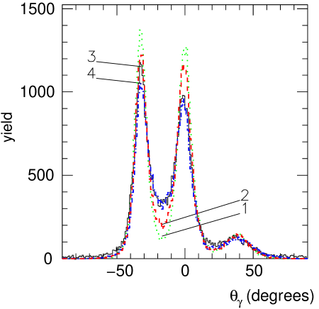
Figure 4: Angular distribution of bremsstrahlung photons. The dotted line (1) (green) and the dashed line (2) (red) represent the simulations using the PA (the difference between the two curves is explained in the caption to fig. 3), and the solid line (3) (black) shows the measured (reconstructed) experimental angular distribution, as in fig. 3. The dot-dashed curve (4) (blue) represents our FAMC simulation (not using the PA; employing method 3 described in the text; see fig. 6). The peaks in $e$ and in $e^{\prime}$ direction generated by the FAMC simulation (4) are broader than the ones from the PA, (1) and (2), and reproduce the data more accurately, especially between the peaks in $e$ and $e^{\prime}$ direction. The height of the $e^{\prime}$ peak is slightly underestimated by the FAMC simulation (4), as well as the large-angle tail beyond the $e^{\prime}$-peak. For details concerning the proton direction see fig. 5. As in fig. 3 both data and simlations are corrected for luminosities and detector efficiencies, and no arbitrary normalization was introduced.

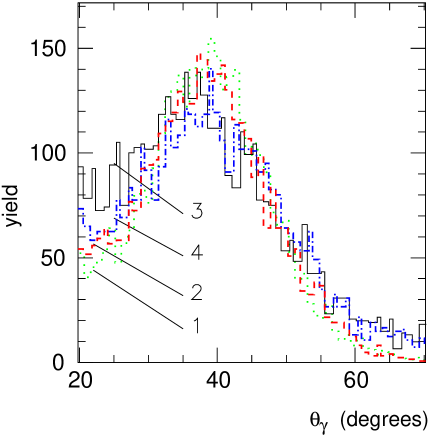
Figure 5: Angular distributions of bremsstrahlung photons. This figure is a cutout of fig. 4, focussing on the region around the proton direction. On the small-angle tail of the proton peak the FAMC simulation (4) does not entirely overcome the gap between simulation and data. However, the region around the proton direction is obscured by punch-throughs.

It is an angle-independent distribution at first but shaped by the rejection algorithm into a contribution which is given by $ee$ interference. There are several ’coin toss’ methods to choose whether an event created from the interference term is assigned to the incoming or the outgoing electron or to both. We employed three different ways of dealing with the interference term, leading to slightly different results. Together with the Monte Carlo photon energy generation (14) and with the photon multiplicity generation (16) each of these three ways of dealing with the interference term constitutes a Monte Carlo event generation method for the interference term.

1. The interference term (being essentially a function of the photon angle $\theta_{\gamma}$) is split into two parts, the ’left part’ consisting of events with angles closer to $\theta_{\rm e}$ and the ’right’ part with angles closer to zero. Events closer to the incoming electron direction (’right’) were counted for the incoming electron whereas events closer to the outgoing electron (’left’) direction were counted for the latter one.

2. In addition to method (1) the energy loss generated using (14) is randomly split between incident and scattered electron.

3. The emitted photon is randomly assigned to either the incoming or the outgoing electron.

For the final comparison between the standard bremsstrahlung treatment (using PA) and our FAMC simulation we used the third method as it fitted the reconstructed photon distribution most accurately, as we will see in the next section.

Once a bremsstrahlung event has been assigned either to the incident electron, the scattered electron or to the struck proton, in mSPA the four-momenta, $k$, $k^{\prime}$, and $p^{\prime}$ are replaced by $k\rightarrow k-\omega$, $k^{\prime}\rightarrow k^{\prime}-\omega$, or by $p^{\prime}\rightarrow p^{\prime}-\omega$, respectively, and the momentum transfer $q^{2}$ is adjusted and inserted into the form factors. $\omega$ is the four-vector of the bremsstrahlung photon.

To check the results produced with our Monte Carlo routine against experimental data we implemented it into the simc code simc developed for Hall C at TJNAF. We used a modified version which was used for the E97-006 $(e,e^{\prime}p)$ experiment daniela . Computation times with and without the new FAMC simulation were similar.

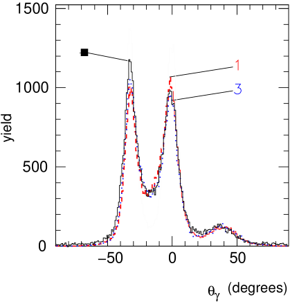
Figure 6: Photon angular distribution for the three different treatments of the interference term (see sec. 3). Method (1) is represented by the dashed line line (red) and it coincides with method (2) (not shown). The dotted line (blue) represents method (3), the solid line (black, marked with the black square) shows the data. Method (3) is found to reproduce the data most accurately and is hence used for the FAMC simulation (4) in fig. 4.

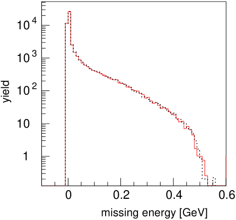
Figure 7: Logarithmic plot of missing-energy distribution. The dotted line (black) was obtained using the PA, the solid line (red) shows the results obtained with the FAMC simulation. The total radiated energy simulated for the latter case is only about 0.3% smaller than the one from the PA. Reasons for this deviation are given at the end of sec. 4.

4 Results

To test our approach we chose H$(e,e^{\prime}p)$ kinematics with a beam energy of $3.12\,{\rm GeV}$. We usually generated 600,000 successful Monte Carlo events per run to compare PA and FAMC simulation. Figs. 4 – 10 show results for the kinematic setting given in table 2.

The photon angles shown in figs. 3 and 4 are obtained according to the prescription

$$\theta_{\gamma}=\arctan\left(\frac{p_{{\rm m}_{y}}}{p_{{\rm m}_{z}}}\right)\,,$$ (22)

where $p_{{\rm m}_{y}}$ and $p_{{\rm m}_{z}}$ are the missing momenta in $y$ and in $z$ direction, respectively. Our co-ordinate system is the one used by SIMC, described in manual .

As pointed out in the introduction, the PA underestimates non-peaked radiation especially between the radiation peaks in the directions of the incident and the scattered electron maximonisabelle0 ; maximonisabelle1 . One can see in fig. 4 that the photon angular distribution broadens when employing the FAMC simulation. The gap between the experimentally determined bremsstrahlung distribution and PA (see fig. 3) between the two radiation peaks in $e$ and $e^{\prime}$ direction is filled.

When calculated with our FAMC method, also the peak in the proton direction fits the reconstructed bremsstrahlung data (see fig. 5). However, this has to be put into perspective as the proton bremsstrahlung is obscured by a detector related artefact (punch-through effects) such that one cannot make a clear statement on the accuracy here.

For the kinematic setting shown in table 2 the $ee$ interference term discussed in the previous section was treated with method (3). This led to the best agreement with data as can be seen in fig. 6. The other two methods also improved the angular distribution of the bremsstrahlung but exhibited a slightly larger deviation from the data concerning the amplitudes of the $e$ and $e^{\prime}$ peaks. At the kinematic setting shown in table 2 the $ee$ interference term accounted for roughly 20% of all events.

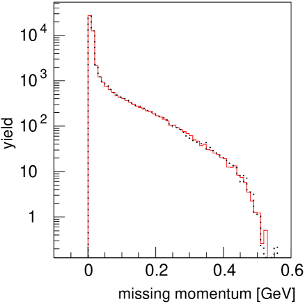
Figure 8: Logarithmic plot of the reconstructed missing-momentum distribution. The missing momentum is almost unaltered. The FAMC simulation is represented by the solid line (red), the PA by the dotted line (black).

Looking at the missing-energy distribution in fig. 7 which includes detector resolution and acceptances, we see that the total FAMC yield is 0.3% smaller than predicted by the PA, while a calculation not taking into account detector resolution and acceptances would yield identical results for FAMC and PA. The 0.3% difference is well within the systematic uncertainty usually attributed to the radiation correction. The missing momenta (see fig. 8) generated by the PA and by our FAMC code do hardly differ either, as the missing energy distribution. The momentum distributions of electron and proton for the kinematics shown in table 2 are also not changed significantly by the FAMC calculations, as can be seen in figs. 9 and 10.

As a further check we also looked at kinematic settings with both larger and smaller values of $Q^{2}$, while we let the beam energy unaltered. We compared again the FAMC simulation with the standard radiation code.

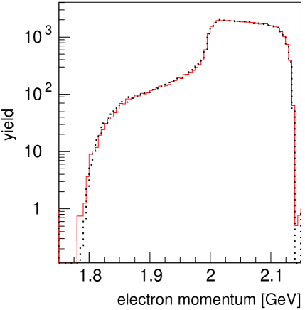
Figure 9: Electron momentum distribution. The dotted line (black) was obtained using the PA, the solid line (red) shows the results using the FAMC simulation.

Looking at the total yield in the acceptance we found differences of up to 3.0%, the yield of the FAMC simulation usually being smaller than the standard analysis yield when going to higher momentum transfers and larger for small values of $Q^{2}$, as can be seen in table 3 and in fig. 11.

The differences in the total yield shown in table 3, in figs. 7 and 11 are related to the inappropriate application of the SPA. It only shows up when including detector simulations into the data analysis.

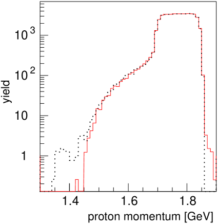
Figure 10: Proton momentum distribution. FAMC simulation (solid line) (red) and peaking calculation (dotted line) (black) almost coincide.

$Q^{2}/$GeV2	0.61⋆	1.00⋆	2.00	3.00⋆	4.00⋆
$|{\bf p^{\prime}}|/$GeV	0.852	1.13	1.70	2.36	2.92
$|{\bf k^{\prime}}|/$GeV	2.74	2.59	2.05	1.52	0.99
$\Delta$ yield	+2.5%	+0.4%	–0.3%	–1.5%	–3.0%

Table 3: The differences in the yield between the standard analysis code and the FAMC simulation, integrated up to $0.7\,{\rm GeV}$. The incident electron’s energy is $k^{0}=3.120\,{\rm GeV}$ for all kinematic settings. Reasons for the differences are given at the end of sec. 4. Missing energy plots for the kinematics settings marked with a star are shown in fig. 11.

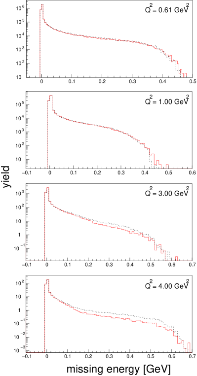
Figure 11: Logarithmic plots of missing-energy distributions for the remaining kinematic settings shown in table 3. The distribution for $Q^{2}=2.00\,{\rm GeV}^{2}$ has already been shown in fig. 7. The solid curves (red) represent the FAMC calculation, the dotted curves (black) show the PA calculation.

Our FAMC approach is more sensitive to problems caused by the SPA than the PA at certain kinematic settings. It uncovers a problem of the SPA which is suppressed by the PA. Including the full angular dependence of bremsstrahlung photons (other than the trivial angular dependence of the PA) can sometimes lead to energy gains for both electron and proton as the particles are assumed to be on-shell. Such un-physical events are rejected by our code, because they are artefacts of the mSPA which corrects for the energy losses due to photon emission and assumes on-shell vertices. At some kinematic settings the un-physical events described above account for a significant fraction of all events, changing the total yield.

The PA does not have this particular problem since it can fulfil both energy and momentum conservation at the same time when assuming massless on-shell electrons. Energy gains through emission of radiation are not possible. The recoiling protons cannot be assumed to be massless, of course. But as they only account for a small fraction of high energy bremsstrahlung events, they do not change the total yield much, neither in the case of the PA nor for the FAMC simulation.

5 The applicability of the SPA

As we have shown in sect. 2 the SPA simplifies the multi-photon bremsstrahlung treatment considerably. In order to evaluate its applicability for the kinematic

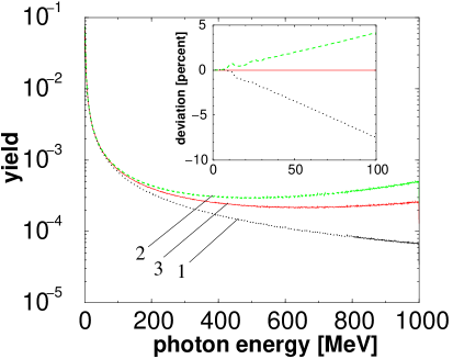
Figure 12: Photon energy distribution for the kinematic setting shown in table 2. The dotted curve (1) (black) represents pSPA where the kinematics used are purely elastic. The dashed curve (2) (green) shows the mSPA calculation which has been corrected for the kinematic changes due to bremsstrahlung. This mSPA has been used in the present paper and also in refs. makins ; simc . The solid curve (3) (red) depicts the exact $1\gamma$ calculation for the photon energy. The inset graph shows the difference between the calculations in percent.

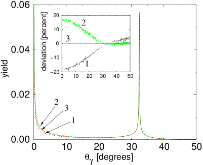
Figure 13: Bremsstrahlung angular distribution for single-photon emission at the kinematic setting shown in table 2. The dotted curve (1) (black) represents pSPA, the dashed curve (2) (green) shows the mSPA calculation, the solid curve (3) (red) depicts the exact $1\gamma$ calculation for the photon angles. The inset graph shows the deviation between the different calculations in percent.

settings considered in this paper we now test the SPA by comparing it to the exact $1\gamma$ calculation (omitting proton bremsstrahlung). The integration over the bremsstrahlung photons is carried out with our FAMC generator. This renders an analytic evaluation of phase space integrals unnecessary.

Let us first describe how we construct a Monte Carlo generator for the exact $1\gamma$ bremsstrahlung calculation from the mSPA Monte Carlo generator described before. Consider the SPA bremsstrahlung cross section

$$\sigma_{\rm SPA} \sim \int\frac{d^{3}\omega}{2\omega^{0}}|{\cal M}_{\rm ep}^{(1)}|^{2}A({\omega})$$ (23)

$$= \int\frac{\omega^{0}d\omega^{0}d\Omega_{\gamma}}{2}|{\cal M}_{\rm ep}^{(1)}|^{2}A({\omega})\,,$$

where we have absorbed the photon energy $\omega^{0}$ into the SPA angular distribution,

$$A(\omega)\equiv\frac{A(\Omega_{\gamma})}{\omega^{0}}\,.$$ (24)

Our FAMC code generates bremsstrahlung events according to the distribution

$$\frac{d^{3}\omega}{2\omega^{0}}A({\omega})=\frac{\omega^{0}d\omega^{0}d\Omega_{\gamma}}{2}A({\omega})\,.$$ (25)

Evaluating the phase space integral in Eq. (23) using our FAMC generator we obtain

$$\sigma_{\rm SPA} \sim \frac{1}{N}\sum_{\rm events}|{\cal M}_{\rm ep}^{(1)}|^{2}A({\omega})\frac{\omega^{0}}{2}\frac{1}{A({\omega})\frac{\omega^{0}}{2}}$$ (26)

$$= \frac{1}{N}\sum_{\rm events}|{\cal M}_{\rm ep}^{(1)}|^{2}\,,$$

where $N$ is the number of events, and ${\cal M}_{\rm ep}^{(1)}$ is the elastic first-order Born matrix element. The exact $1\gamma$ calculation (not using the SPA) yields

$$\sigma_{1\gamma}\sim\int\frac{\omega^{0}d\omega^{0}d\Omega_{\gamma}}{2}|{\cal M}_{1\gamma}|^{2}\,,$$ (27)

where

$${\cal M}_{1\gamma}={\cal M}_{\rm ei}+{\cal M}_{\rm ef}$$ (28)

is the exact QED single-photon electron bremsstrahlung amplitude. The cross section (27) becomes

$$\sigma_{1\gamma} \approx \frac{1}{N}\sum_{\rm events}\frac{|{\cal M}_{1\gamma}|^{2}}{2}\frac{1}{\frac{A({\omega})}{2}}$$ (29)

$$= \frac{1}{N}\sum_{\rm events}\frac{|{\cal M}_{1\gamma}|^{2}}{A({\omega})}$$

in the Monte Carlo formalism. In order to measure the applicability of the SPA we assign a weight $w_{\rm ex}$ to each event, defined by the ratio of the squared matrix elements from eqs. (26) and (29), re-weighting our FAMC generator (SPA),

$$w_{\rm ex}\equiv\frac{|{\cal M}_{1\gamma}|^{2}}{|{\cal M}_{\rm ep}^{(1)}|^{2}A(\omega)}\,.$$ (30)

We compare that weight with the mSPA weight

$$w_{\rm mod}\equiv\frac{|{\cal M}_{\rm ep}^{\rm(1),\,mod}|^{2}A^{\rm mod}({\omega})}{|{\cal M}_{\rm ep}^{(1)}|^{2}A(\omega)}\,,$$ (31)

where ’mod’ indicates that these matrix elements in the numerator have been calculated for modified kinematics, i.e. in mSPA. Finally we define the trivial weight

$$w_{\rm triv}\equiv\frac{|{\cal M}_{\rm ep}^{(1)}|^{2}A({\omega})}{|{\cal M}_{\rm ep}^{(1)}|^{2}A(\omega)}=1\,,$$ (32)

which represents the pSPA, i.e. the pure SPA calculation not taking into account any kinematic changes imposed by emission of bremsstrahlung. This last option is the roughest approximation. A version of the mSPA represented by weight (31) is also used in ref. makins , combined with the PA.

Plotting the photon energy distribution (see fig. 12) using the three weights (30), (31), and (32) for each Monte Carlo event, we see that the deviation between the mSPA calculation and the $1\gamma$ calculation for the photon energy is 4.1% for $\omega^{0}=100\,{\rm MeV}$. The deviation becomes much larger for higher energies, going up to 90% for photon energies of $\omega^{0}=1000\,{\rm MeV}$, the mSPA calculation makins ; simc overestimating the radiative tail; and one can find even larger deviations for different kinematic settings. However, bremsstrahlung events with photon energies of several hundred MeV are unimportant for the data analyses since the particle detectors do not see them. Their momentum acceptances usually are limited to $\pm 10\%$ of the central (elastic) momenta, depending on what one is looking for.

The dotted curve (1) in fig. 12 shows the pSPA which was obtained using weight (32). Most data analysis codes make use of some version of the mSPA. The mSPA is closer to the exact calculation than pSPA, so it constitutes an improvement over pSPA. This finding is in agreement with ref. makins .

For our purposes the influence of the SPA on the photon angular distribution is more important than the deviation in the missing energy calculation. Fig. 13 shows the photon angular distribution. The largest deviations occur in the vicinity of the peak due to radiation from the incident electron, at small values of the angle $\theta_{\gamma}$. While the $1\gamma$ calculation of the bremsstrahlung cross section is symmetric in $e$ and $e^{\prime}$, the mSPA data analysis procedures are not, resulting in asymmetric deviations from the $1\gamma$ result. This can be understood from the energy loss of the incident electron, leading to smaller bremsstrahlung energies coming from the scattered electron. From fig. 3 we know that one critical domain of large discrepancies between data and standard simulations using the PA is the region in the middle between the two radiation peaks where the PA angular distribution falls below the measured distribution by a factor 2. Fig. 13 shows that the FAMC calculation (using mSPA) overestimates the photon angular distribution in this region by 13%. Fig. 4 however suggests, that the FAMC (using mSPA) reproduces the data well, especially in the region in the middle between the two radiation peaks. Comparing fig. 4 (which includes internal and external bremsstrahlung, multi-photon emission, finite detector resolution and acceptances, multiple scattering and other energy losses) and fig. 13 (internal single-photon bremsstrahlung only) in the critical region between the two electron radiation peaks, we can conclude that the SPA impact on the angular distribution is smeared out by other sources of inaccuracies like finite detector resolution, finite momentum acceptances, and multiple scattering.

In fig. 4 we saw that the height of the $e^{\prime}$ peak is slightly underestimated by our FAMC simulation, as well as the large-angle tail beyond the $e^{\prime}$ peak. The results shown in fig. 13 indicate small differences between the mSPA and the exact $1\gamma$ calculation in the vicinity of the $e^{\prime}$ peak only. And also the difference in fig. 13 at the large-angle tail beyond the $e^{\prime}$ peak is small. At this stage it is not entirely clear whether removal of the SPA would affect the photon angular distribution in these regions.

6 Conclusion and Outlook

Using a FAMC bremsstrahlung calculation at almost no extra computational expense improves the treatment of internal bremsstrahlung in $(e,e^{\prime}p)$ experiments. One shortcoming of the PA, the underestimation of bremsstrahlung between the radiation peaks, is solved by our approach. We have also shown how the PA can be removed.

Figs. 7 and 11 and table 3 indicated that the FAMC simulation exposes problems due to the SPA which are hidden when using the PA. And while for the photon angular distribution the PA may be the dominant source of error, we have shown in the previous section that the SPA seems to have a sizeable influence on the missing energy distribution.

These two problems with the SPA indicate that it would be desirable to also remove the SPA from data analysis codes. But there are several problems which have to be tackled in order to achieve such an improved calculation. An exact multi-photon calculation would be impracticable since one would have to insert the QED cross sections into the analysis codes for multi-photon bremsstrahlung up to arbitrarily high orders. One could instead try to combine exact single-photon bremsstrahlung for the hardest bremsstrahlung photon with SPA multi-photon emission for the softer photons in order to improve the present bremsstrahlung treatment. Yet, inclusion of proton bremsstrahlung, as in the present paper, seems not to be feasible for such calculations.

- (1) J. Schwinger, Phys. Rev. 75, 898 (1949); J. Schwinger, Phys. Rev. 76, 790 (1949)
- (2) Y. S. Tsai, Phys. Rev. 122, 1898 (1961)
- (3) L. I. Schiff, Phys. Rev. 87, 750 (1952)
- (4) D. R. Yennie, S. C. Frautschi, H. Tsuura, Ann. Phys. 13, 379 (1961)
- (5) L. C. Maximon, D. B. Isabelle, Phys. Rev. 133 B, 1344 (1964)
- (6) L. C. Maximon, D. B. Isabelle, Phys. Rev. 136 B, 764 (1964)
- (7) L. C. Maximon, Rev. Mod. Phys. 41, 193 (1969)
- (8) L. W. Mo, Y. S. Tsai, Rev. Mod. Phys. 41, 205 (1969)
- (9) E. Borie, D. Drechsel, Nucl. Phys. A 167, 369 (1971)
- (10) E. Borie, Z. f. Naturforschung, 30a, 1543 (1975)
- (11) J. Friedrich, Nuclear Instruments and Methods 129, 505 (1975)
- (12) C. de Calan, H. Navelet, J. Picard, Nucl. Phys. B 348, 47 (1991)
- (13) A. Akhundov, D. Bardin, L. Kalinskaya, T. Riemann, Phys. Lett. B 301, 447 (1993), hep-ph/9507278; A. Akhundov, D. Bardin, L. Kalinskaya, T. Riemann, Fortschr. Phys. 44, 373 (1996), hep-ph/9407266
- (14) J. A. Templon, C. E. Vellidis, R. E. J. Florizone, A. J. Sarty, Phys. Rev. C 61, 014607 (2000)
- (15) L. C. Maximon, J. A. Tjon, Phys. Rev. C 62, 054320 (2000)
- (16) A. Afanasev, I. Akushevich, N. Merenkov, Phys. Rev. D 64, 113009 (2001), hep-ph/0102086
- (17) A. Afanasev, I. Akushevich, A. Ilyichev, N. P. Merenkov, Phys. Lett. B 514, 269 (2001), hep-ph/0105328
- (18) R. Ent et al., Phys. Rev. C 64, 054610 (2001)
- (19) A. Afanasev, I. Akushevich, A. Ilyichev, B. Niczyporuk Czech. J. Phys. 53, B449 (2003), hep-ph/0308106
- (20) J. Arrington, private communication on simc 2001 release, TJNAF; P. E. Ulmer, private communication on mceep, release 3.8, TJNAF; simc and mceep manuals, available from TJNAF website
- (21) S. N. Gupta, Phys. Rev. 99, 1015 (1955)
- (22) M. Vanderhaeghen et al., Phys. Rev. C 62, 025501 (2000)
- (23) D. Rohe et al., Eur. Phys. J. A 17, 439 (2003)
- (24) R. R. Lewis, Phys. Rev. 102, 537 (1956)
- (25) S. D. Drell, M. A. Ruderman, Phys. Rev. 106, 561 (1957)
- (26) S. D. Drell, S. Fubini, Phys. Rev. 113, 741 (1959)
- (27) J. A. Campbell, Phys. Rev. 180, 1541 (1969)
- (28) P. G. Blunden, W. Melnitchouk, and J. A. Tjon, Phys. Rev. Lett. 91, 142304 (2003)
- (29) P. A. M. Guichon and M. Vanderhaeghen, Phys. Rev. Lett. 91, 142303 (2003)
- (30) G. ’t Hooft, Nucl. Phys. B 61, 455 (1973)
- (31) Hall C Physics Vade Mecum; J. Arrington, A-B-SIMC, TJNAF (2001)