Recent Developments in the Lorentz Integral Transform (LIT) Method

Abstract

Recent results on electromagnetic (e.m.) reactions into the continuum of systems with A from 3 to 7 are presented. They have been obtained using the LIT method (ELO94, ). The method is shortly reviewed, emphasizing how all the results, though obtained with the sole ingredient of the N-N potential, contain the full complicated dynamics of the A-body system, both in the initial and in the final states.

1 The LIT method

The LIT method is suited for ab initio studies of few (many) body dynamics in the framework of non relativistic quantum mechanics. The inputs are the nuclear potential and the excitation operator relevant to the reaction. Even if the reaction brings the system to a continuum state one does not need to calculate continuum wave functions. What the method allows to calculate are matrix elements (or combinations of them) to continuum states, which is what one needs in order to evaluate cross sections.

Essential to the method are solutions of the Schrödinger equation for the ground state and of a Schrödinger-like equation with a source. In both cases the solutions have bound-state asyntotic conditions. So in order to apply the LIT method one only needs a ”good” technique for bound state calculations.

The LIT method applies both to inclusive reactions and to exclusive ones. In a traditional approach the former case is considered more complicated, because of the necessity to know solutions for all the disintegration channels. However, it turns out that the application of the LIT method is more straightforward in this case than in an exclusive reaction. The LIT method has been benchmarked in 2- and 3-body systems where continuum states can be calculated directly ELO94 ; Lapiana ; Martinelli ; Golak

The procedure of the LIT method, though similar in spirit, is different for inclusive and exclusive reactions. In the following I will list the main steps one has to take in the two cases.

1.1 Inclusive Reactions

For inclusive e.m. reactions one needs to know the so called response function

$$R(\omega)=\sum\!\!\!\!~{}\!\!\!\!\!\!\!\!\int_{n}|\langle 0|\Theta|n\rangle|^{2}\delta(\omega-E_{n}+E_{0})$$ (1)

where $\omega$ represents the energy transferred by the elctromagnetic probe, $|0>$ and $E_{0}$ are ground state wave function and energy of the system undergoing the reaction, $|n>$ and $E_{n}$ are all the eigenstates and eigenvalues of the Hamiltonian $H$ and $\Theta$ is the operator relevant to the reaction. In order to calculate $R(\omega)$ one proceeds in three steps.

Step 1. The first step consists in solving for many $\omega_{0}$ and fixed $\Gamma$ the following equation

$$(H-E_{0}-\omega_{0}+i\Gamma)\tilde{\Psi}=\Theta|0>$$ (2)

The values of the parameters $\omega_{0}$ and $\Gamma$ are chosen in relation to the physical problem. For example, if one wants to calculate the cross section in a range of energies from 0 to 100 MeV one solves that equation with $\Gamma\simeq$10 MeV for about 100 $\omega_{0}$ values chosen in a range slightly larger than 100 MeV, e.g. $100+2\Gamma$ MeV. As it will be clear below the value of $\Gamma$ is related to the kind of resolution one wishes to have in order to to resolve the expected structures of the response function and the values of $\omega_{0}$ scan the region of interest.

Step 2. The second step consists in calculating the overlaps $<\tilde{\Psi}|\tilde{\Psi}>$ of the solutions. Of course these overlaps depend on $\omega_{0}$ and $\Gamma$. A theorem based on the closure property of the Hamiltonian eigenstates ensures that this dependence can be expressed as ELO94

$$<\tilde{\Psi}|\tilde{\Psi}>=\int R(\omega)\,L(\omega,\omega_{0},\Gamma)\,d\omega$$ (3)

where $L(\omega,\omega_{0},\Gamma)$ is the Lorentzian function centered at $\omega_{0}$ and with $\Gamma$ as width. Therefore if one solves Eq. (1) one can easily obtain the Lorentz integral transform of the response function.

Step 3. The third step consists in the inversion of this transform in order to obtain the response function.

1.2 Exclusive Reactions

For exclusive reactions the LIT method is applied Lapiana ; Quaglioni to calculate the relevant transition matrix element $<\Psi(E)|\Theta|0>$, where $\Psi(E)$ is the wave function in the continuum at energy E. As already said, in this case, the procedure requires more steps.

Step 1. The first step is identical to the case of inclusive reactions i.e. one has to solve Eq.(1). Now the choice of the parameters is dictated by different criteria. I will comment on this after describing the last step.

Step 2. There is a second Schrödinger like equation with source to be solved for exclusive reactions. For example, in the case of a 2-body break-up reaction this is

$$(H-E_{0}-\omega_{0}+i\Gamma)\tilde{\Psi}_{2}=V|0>$$ (4)

where V is the potential acting between the particles belonging to the two different fragments.

Step 3. The third step consists in calculating the overlap $<\tilde{\Psi}|\tilde{\Psi}_{2}>$. Again, for a theorem based on the closure property of the Hamiltonian eigenstates, this overlap is connected via a LIT to the important function $F(E)$ Lapiana ; efros85

$$<\tilde{\Psi}|\tilde{\Psi}_{2}>=\int F(E)\,L(E,\omega_{0},\Gamma)\,dE$$ (5)

As it will be clear in step 5 this function is what one needs to calculate the matrix element of interest.

Step 4. In order to obtain F(E) one has to invert the previous Lorentz transform and proceed to the final step.

Step 5. It is easy to show Lapiana ; efros85 that the matrix element of interest is connected to the function $F(E)$ via the following integral

$$<\Psi(E)|\Theta|0>=\int dE^{\prime}\,{F(E^{\prime})\over(E-E^{\prime}+i\epsilon)}$$ (6)

This equation suggests the physical criteria one has to follow in the choice of the parameters $\omega_{0}$ and $\Gamma$ entering Eqs.(1) and (4). Since the reaction matrix element is taking its major contribution from $F(E^{\prime})$ at $E^{\prime}=E$ a good knowledge of $F(E^{\prime})$ is needed around the $E$ value. This means that its Lorentz transform needs to be known in a large enough range around that value and for small enough width in order to obtain an accurate function when inverting it.

Important remarks regarding the solutions of Eqs.(1) and (4) and about the inversion of the LIT will be done in the next section.

1.3 Important Remarks

At this point it should be clear that the main points of the LIT method lay in Eqs. (1) and (4). One can easily show that the solution of these equations is unique. Moreover a very important point is that, due to the presence of a complex energy and sources which asyntotically vanish the solutions are limited i.e. of bound state type (this is certainly the case for all physical e.m. operators and for the nuclear potential V in Eq.(4); for long range potentials a different procedure is requred Lapiana ). This has the very important consequence that one only needs bound state techniques (notice that also the ground state is an input of Eqs. (1) and (4)) in order to solve the problem of calculating a reaction in the continuum, even when many complicated channels are opened, like for inclusive cases above the thresholds.

An other remark concerns the inversion of the transforms. Due to the bell shaped form of the kernel, the inversions turn out to be rather stable. Of course for any inversion technique one can use (we use the regularization method book ) one has to check that the same result for different choices of $\omega_{0}$ sets and values of $\Gamma$ is obtained.

In the following I will present results which have been obtained using the Correlated Hyperspherical Harmonics (CHH CHH ) and the Effective Interaction in the Hyperspherical Harmonics expansions (EIHH EIHH ) techniques to solve the bound sate problems and both semirealistic (MTI-III MT and AV4’ AV4' ) and realistic (AV18+UIX AV18UIX ) potentials.

2 results

I start showing results for the 3-body systems 3body . In Fig. 1a the longitudinal responses of ³H and ³He are shown. The effect of the 3-body force is visible in the quasi elastic (q.e.) peak. While the 3-body potential seems to be necessary for a better agreement with data in the case of ³He, it brings the curves farer from them in the tritium case. The comparison with data at higher momentum transfers $q$ is of the same quality 3body .

Figure 1: Longitudinal electron scattering responses of 3-body systems. LIT results in unretarded E1 approximation with AV18 only (dashed curves) and with AV18+UIX (full curve).(a): q.e. region, data from saclay ; bates . (b): low energy region, data from retzlaff , dotted curve: result from Viviani

Fig. 1b shows the situation at lower energies. The discrepancy at the highest $q$ is worsened by considering the 3-body interaction. More precise data would be needed to study 3-body force effects.

An interesting effect is shown in Fig. 2 where the frame dependence of the results is shown. Performing the calculation in the laboratory system, (where the total momentum of the initial state is at rest) or in the anti-laboratory one (where the total momentum of the final state is at rest) or in the Breit frame (where the total momenta of the initial and final states are equal to $q/2$) brings to a visible shift of the q.e. peak at higher momenta. This shows the limits of the non realtivistic calculation. Data seem to agree better with the results obtained in the Breit frame.

In Table 1 results for the longitudinal 2-body electrodisintegration of ⁴He are shown Quaglioni for the kinematics of Ref.ducret represented in the ($q-\omega$) plane and labelled by arabic numbers in Fig 3. The different effects of proper antisymmetization (AS) and of the interaction in the final state (FSI), neglected in the direct knock-out plane wave approximation (PWIA), are shown. In general one notices small effects of the antisymmetrization for almost all cases, as one would expect in parallel kinematics. Nevertheless for the kinematics at lower energies these effects can increase up to about 10%. The role of FSI is much more important, especially at low $q$. It seems to decrease considerably at $q$ beyond 500 MeV/c. All these results have been obtained with the semirealistic MTI-III potential (more details can be found in the poster contribution to this conference sofia ). Results for the 4-body system with AV18+UIX potential have been obtained in the inclusive case (total photodisintegration) and are also shown as poster contribution to this conference doron

Figure 2: Frame dependence of the longitudinal electron scattering responses of triton calculated in the laboratory system (LAB), or in the anti-laboratory one (AL) or in the Breit frame.

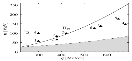
Figure 3: Values of momentum $q$ and energy transfer $\omega$ for the kinematics of Ref. ducret . See Table 1.

Table 1: Results for the longitudinal 2-body electrodisintegration response function $R_{L}$ of ⁴He. In the first 3 columns the kinematical values of momentum $q$, energy transfer $\omega$ and missing momentum $p_{m}$ from Ref. ducret . The AS and FSI effects are shown as percentages of the PWIA values

Kin.	$q$	$\omega$	$p_{m}$	$R_{L}(PWIA)$	AS	AS+FSI
No.	[MeV/c]	[MeV]	[MeV/c]	[(GeV/c)-3 sr-1]	$\%$	$\%$
1	299	57.78	+30	110.1	+10.9	-45
2	380	83.13	+30	83.7	+2.0	-25
3	421	98.19	+30	72.0	+0.7	-18
4	299	98.70	-90	61.6	+1.9	-35
5	380	65.06	+90	44.6	+7.5	-37
6	544	126.6	+90	23.2	-0.1	+0.6
7	572	137.82	+90	20.6	-0.2	+3.4
8	650	175.67	+90	14.7	-0.2	+7.3
9	680	146.68	+190	1.79	-0.4	+28.8

In Fig. 4a results for the total photodisintegration of the 6-body systems are shown 6body . The unretarded electric dipole operator is used. A very interesting feature i.e. the appearance of two resonances in the case of ⁶He is worth to be noticed. They likely correspond to the soft mode due to theoscillation of the two halo neutrons against the alpha-core and to the classical giant resonance mode of protons against neutrons, respectively. Since the latter requires the break-up of the alpha core the resonance appears at higher energy. One finds a unique resonance in ⁶Li, though also in this case one would expect two, due to the probable clusterized form of this nucleus. An explanation for the disappearence of the dip between the two resonances might be that in this case an additional mode i.e. the ³H-³He oscillation is filling the gap. An analogous ³H-³He mode in ⁶He would not be excited by the dipole operator. New accurate 2-body break up data of ⁶Li would be needed to confirm this hypothesis.

(a)

Figure 4: Faddeev (dots) and LIT result (upper and lower bounds, full curves) in unretarded E1 approximation and for AV18 potential. From bench02.

(b)

Figure 5: (a): total photoabsorption cross sections of ⁶Li and ⁶He for different potential models MT ; AV4' ; MN . (b): total photoabsorption cross section of ⁷Li compared to data of Ref. ahrens .

Finally in Fig. 4b it is shown how the LIT method presently allows to calculate an inclusive reaction involving 7 particles fully ab initio. This result for the total photoabsorption of ⁷Li is commented in more detail in another contribution to this conference 7body

References

- (1) Efros V.D., Leidemann W., and Orlandini G., Phys. Lett. B 338, 130-133 (1994).
- (2) Efros V.D., Leidemann W., and Orlandini G., Few-Body Syst. 26, 251-269 (1999).
- (3) La Piana A. and Leidemann W., Nucl. Phys. A677, 423-441 (2000).
- (4) Martinelli S., Kamada H., Orlandini G. and Glöckle W., Phys. Rev. C 52, 1778-1782 (1995).
- (5) J. Golak et al., Nucl. Phys. A707, 365-378 (2002).
- (6) Quaglioni S., Leidemann W., Orlandini G., Barnea N. and Efros V.D., Phys. Rev. C 69, 044002-1-8 (2004).
- (7) Efros V.D., Yad. Fiz. 41, 1498 (1985) [Sov. J. Nucl. Phys. 41, 949 (1985)]; Yad. Fiz. 62, 1975 (1999) [Phys. Atom. Nucl. 62, 1833 (1999)].
- (8) Tikonov A.N. and Arsenin V.Ya., Solution of Ill Posed Problems, New York: Halsted 1973.
- (9) Fenin Yu. I. and Efros V.D., Yad. Fiz. 15, 887 (1985) [Sov. J. Nucl. Phys. 15, 497 (1972)]Yad.; Rosati S., Kievsky A. and Viviani M., Few-Body Systems Suppl., 7 278 (1994).
- (10) Barnea N., Leidemann W. and Orlandini G., Phys. Rev. C 61, 054001-1-10 (2000); Barnea N., Leidemann W. and Orlandini G., Nucl. Phys. A693, 565-578 (2001).
- (11) Malfliet R.A., Tjon J., Nucl. Phys. A127, 161-168 (1969).
- (12) Wiringa R.B. and Pieper S.C., Phys. Rev. Lett. 89, 182501-4 (2002).
- (13) Wiringa R.B., Stoks V.G.J. and Schiavilla R., Phys. Rev. C 51, 38-51(1995); Pudliner B.S., Pandharipande V.R., Carlson J., Pieper S.C. and Wiringa R.B., Phys. Rev. C 56, 1720-1750 (1997).
- (14) Efros V.D., Leidemann W., Orlandini G. and Tomusiak E.L., Phys. Rev. C 69, 044001-1-10 (2004).
- (15) Marchand C. et al., Phys. Lett. B 153, 29 (1985); Morgenstern J., private communications.
- (16) Dow K. et al., Phys. Rev. Lett. 61, 1706-1709 (1988).
- (17) Retzlaff G.A., et al., Phys. Rev. C 49, 1263-1271 (1994).
- (18) Viviani M., Kievsky A., Marcucci L.E., Rosati S. and Schiavilla R., Phys. Rev. C 61, 064001-1-18 (2000).
- (19) Ducret J.E. et al., Nucl. Phys. A556, 373-395 (1993).
- (20) Quaglioni S., Efros V.D., Leidemann W. and Orlandini G., poster contribution to this conference.
- (21) Barnea N., Gazit D., Leidemann W. and Orlandini G., poster contribution to this conference.
- (22) Bacca. S., Marchisio M.A., Barnea N., Leidemann W. and Orlandini G., Phys. Rev. Lett 89, 052502-1-4 (2002); Bacca. S., Barnea N., Leidemann W. and Orlandini G., Phys. Rev. C 69, 057001-1-4 (2004).
- (23) Thomson D.R., LeMere M. and Tang Y.C., Nucl. Phys. A286, 53-66 (1977); Reichstein I. and Tang Y.C., ibid., A158, 529 (1970).
- (24) Bacca. S., Arenhövel H., Barnea N., Leidemann W. and Orlandini G., nucl-th/0406080.
- (25) Ahrens J. et al., Nucl. Phys. A251, 479-492 (1975).