FZJ–IKP(TH)–2004–19, HISKP-TH-04-22

Flatté-like distributions and the $a_{0}(980)/f_{0}(980)$ mesons

Abstract

We explore the features of Flatté-like parametrizations. In particular, we demonstrate that the large variation in the absolute values of the coupling constants to the $\pi\eta$ (or $\pi\pi$) and $K\bar{K}$ channels for the $a_{0}$(980) and $f_{0}$(980) mesons that one can find in the literature can be explained by a specific scaling behaviour of the Flatté amplitude for energies near the $K\bar{K}$ threshold. We argue that the ratio of the coupling constants can be much better determined from a fit to experimental data.

1 Introduction

In spite of a long history of investigations since their discovery the nature of the light scalar mesons $f_{0}(980)$ and $a_{0}(980)$ is far from being understood Buggrep ; Klempt ; Torn ; Oller ; Bev ; Ani . Usually to get information about the properties of these resonances the so-called Flatté parametrization Flatte for the differential mass distributions is used. This parametrization was first introduced by Flatté for the description of the $\pi\eta$ invariant mass distribution near the $K\bar{K}$ threshold where the $a_{0}(980)$ scalar-isovector resonance is located.

The Flatté differential mass distribution is a slightly modified relativistic version of the Breit-Wigner distribution. It reads, e.g., for the $a_{0}$ channel

$$\frac{d\sigma_{i}}{dm}\propto\left|\frac{m_{R}\sqrt{\Gamma_{\pi\eta}\Gamma_{i}}}{m_{R}^{2}-m^{2}-im_{R}(\Gamma_{\pi\eta}+\Gamma_{K\bar{K}})}\right|^{2},$$ (1)

with the partial widths $\Gamma_{\pi\eta}=\bar{g}_{\eta}q_{\eta}$ and

$$\Gamma_{K\bar{K}}=\bar{g}_{K}\sqrt{m^{2}/4-m^{2}_{K}}$$

above threshold and

$$\Gamma_{K\bar{K}}=i\bar{g}_{K}\sqrt{m_{K}^{2}-m^{2}/4}$$

below threshold, respectively. The subscript $i$ in Eq. (1) labels the $\pi\eta$ and/or $K\bar{K}$ channels. Furthermore, $m_{R}$ is the nominal mass of the resonance, $m$ is the invariant mass ($m^{2}=s$) and $q_{\eta}$ is the corresponding center-of-mass momentum in the ${\pi\eta}$ system. $\bar{g}_{\eta}$ and $\bar{g}_{K}$ are dimensionless coupling constants that are related to the dimensional coupling constants $g_{\pi\eta}$ and $g_{K\bar{K}}$ commonly used in the literature by $\bar{g}_{\eta}=g^{2}_{\pi\eta}/(8\pi m^{2}_{R})$ and $\bar{g}_{K}=g^{2}_{K\bar{K}}/(8\pi m^{2}_{R})$, respectively.

Since the position of the $a_{0}$ peak is located far from the $\pi\eta$ threshold and the peak is relatively narrow, we may consider the inelastic width $\Gamma_{\pi\eta}$ to be approximately constant for energies near the $K\bar{K}$ threshold. The width $\Gamma_{K\bar{K}}$, on the other hand, varies rapidly near this threshold. The shape of the Flatté distribution (1) is determined by three free parameters $m_{R}$, $\Gamma_{\pi\eta}$ (or $\bar{g}_{\eta}$) and $\bar{g}_{K}$, which should be fixed from a fit of Eq. (1) to the experimental differential mass distribution. As was stressed already in Ref. Flatte , if the value of $\bar{g}_{K}$ is reasonably large, then the $\Gamma_{K\bar{K}}$ term in the denominator of Eq. (1) will suppress the cross section for masses below the $K\bar{K}$ threshold, thus narrowing the $\pi\eta$ mass distribution. It was also mentioned in Ref. Flatte that “the differences between the shapes with $\Gamma_{\pi\eta}$ = 80 MeV and $\Gamma_{\pi\eta}$ = 300 MeV are relatively slight”.

More than two decades have passed since the paper by Flatté and a wealth of different experimental data concerning the $f_{0}(980)$ and $a_{0}(980)$ resonances has been obtained in the meantime. Nevertheless the uncertainties in the parameters extracted for both resonances remain large! To demonstrate this we compile in Tables 1 and 2 some results of analyses for the $a_{0}$ Teige ; Bugg ; Amsler ; SNDa ; KLOEa ; AchKi and $f_{0}$ SND ; CMD2 ; KLOE ; E791 ; WA102 ; OPAL mesons where Flatté or Flatté-like parametrizations like the one by Achasov (see, e.g. Refs. AchKi ; AchGu and references therein) are utilized. Note that these different parameterizations are equivalent in the nonrelativistic limit, i.e. near the $K\bar{K}$ threshold, which means that they all lead to the same analytical form and the parameters of a particular distribution can be re-expressed by those of the other distribution. We show this explicitly for Achasov’s distribution in Appendix.

Table 1 clearly demonstrates, for the $a_{0}$ meson, that the resulting absolute values of $\bar{g}_{\eta}$ ($\Gamma_{\pi\eta}$) and $\bar{g}_{K}$ differ significantly for different analyses. At the same time it also reveals that the ratios of the coupling constants, $R=\bar{g}_{K}/\bar{g}_{\eta}=g_{K\bar{K}}^{2}/g_{\pi\eta}^{2}$, are more or less consistent with each other for practically all the parameter sets extracted from the experimental data. For the $f_{0}(980)$ meson the situation is very similar for most of the results shown in Table 2. We should mention that in case of the results of Refs. E791 ; OPAL for the $f_{0}$ and of Ref.SNDa for the $a_{0}$, which deviate so strongly from the general trend, the value of $\bar{g}_{K}$ is afflicted with large errors, cf. Ref. SNDa ; E791 ; OPAL .

In the present paper we investigate the features of Flatté or Flatté-like parametrizations. In the course of this we demonstrate that the relative stability for the ratio $R$ and the large variations in the absolute values of the coupling constants and masses, evidenced by the different fits as mentioned above, can be understood. It is simply a consequence of a specific scaling behaviour of the Flatté amplitude for energies near the $K\bar{K}$ threshold. The corresponding scale transformation is introduced in Sect. 2 and we discuss its implications for the elastic (i. e. $\pi\pi$ or $\eta\pi$) scattering amplitude near the $K\bar{K}$ threshold and for the effective range parameters of the $K\bar{K}$ channel.

In Sect. 3 we focus on the interplay between resonance structure and threshold. In particular, we investigate the movement of the poles as a function of the coupling strength to the $K\bar{K}$ channel and we examine the corresponding results for the ($\pi\pi$ or $\eta\pi$) scattering amplitude and phase shifts.

Sect. 4 deals with the concrete cases of the $a_{0}$(980) and $f_{0}$(980) mesons. Employing various Flatté parametrizations for those mesons from the literature we exemplify that the resulting phase shifts are indeed very similar for most parameter sets, despite of the fact that the resonance parameters themselves differ drastically. Thus, the actual results for the $a_{0}$(980) and $f_{0}$(980) clearly reflect the typical scaling behaviour that we derived for such Flatté-type parametrizations. The paper ends with some concluding remarks.

Ref.	$m_{R}$	$\Gamma_{\pi\eta}$	$\bar{g}_{\eta}$	$\bar{g}_{K}$	$R$	$E_{R}$	$\alpha$
Teige	1001	70	0.218	0.224	1.03	9.6	0.276
Bugg	999	143	0.445	0.516	1.16	7.6	0.106
Amsler	999	69	0.215	0.222	1.03	7.6	0.221
SNDa a	995	125	0.389	1.414	3.63	3.7	0.027
KLOEa a	984.8	121	0.376	0.412	1.1	-6.5	-0.28
AchKi a	1003	153	0.476	0.834	1.75	11.6	0.096
AchKi a	992	145.3	0.453	0.56	1.24	0.6	0.006

Table 1: Flatté parameters for the $a_{0}$(980) meson taken from the literature. The values of $m_{R}$, $\Gamma_{\pi\eta}$ and $E_{BW}$ are given in MeV. Values for Refs. labeled with the superscript ^a are based on Achasov’s parametrization AchKi , cf. also the Appendix.

Ref.	$m_{R}$	$\Gamma_{\pi\pi}$	$\bar{g}_{\pi}$	$\bar{g}_{K}$	$R$	$E_{R}$	$\alpha$
SND a	969.8	196	0.417	2.51	6.02	-21.5	-1.35
CMD2 a	975	149	0.317	1.51	4.76	-16.3	-1.00
KLOE a	973	256	0.538	2.84	5.28	-18.3	-1.07
E791	977	42.3	0.09	0.02	0.22	-14.3	-0.66
WA102	–	90	0.19	0.40	2.11	–	–
OPAL	957	42.3	0.09	0.97	10.78	-34.3	-1.60

Table 2: Flatté parameters for the $f_{0}$(980) meson taken from the literature. The values of $m_{R}$, $\Gamma_{\pi\eta}$ and $E_{BW}$ are given in MeV. Values for Refs. labeled with the superscript ^a are based on Achasov’s parametrization AchKi , cf. also the Appendix.

2 The Flatté distribution and scaling behaviour

Let us concentrate here on energies near the $K\bar{K}$ threshold. In this region the resonance part of the elastic scattering amplitude for the channel with the light particles ($\pi\eta$ for the $a_{0}$(980) case or $\pi\pi$ for the $f_{0}$(980) meson) can be written in a nonrelativistic form by

$$f_{el}=-\frac{1}{2q}\frac{\Gamma_{P}}{E-E_{BW}+i\frac{\Gamma_{P}}{2}+i\bar{g}_{K}\frac{k}{2}}\ .$$ (2)

This nonrelativistic expression can be derived starting out both from the relativistic Flatté formula (see Eq.(1)) and from the Flatté-like distributions like the one introduced by Achasov AchKi which takes into account the so called finite width corrections due to $\pi\eta$ (or $\pi\pi$) and $K\bar{K}$ loops (see Appendix for more details). Here we use the notation $\Gamma_{P}=q\bar{g}_{P}$ for the inelastic width, where $P$ stands for the ${\pi\eta}$ or ${\pi\pi}$ channels and $q$ is the corresponding center-of-mass momentum. The energies are defined with respect to the $K\bar{K}$ threshold, i.e.

$$E =\sqrt{s}-2m_{K},\ \ m_{R}=2m_{K}+E_{R},$$ (3)

where $\displaystyle m_{K}=({m_{K^{+}}+m_{K_{0}}})/{2}$ and $m_{R}$ is the nominal mass of the resonance. The parameter $E_{BW}$, which would correspond to the peak position of the standard nonrelativistic Breit-Wigner (BW) resonance, i.e. in the limit $\bar{g}_{K}\to 0$, is defined as

$$E_{BW}=E_{R}$$

for the Flatté distribution ($E_{BW}$ for the Achasov distribution is defined by Eq. (26) in the Appendix). In addition the relative $K\bar{K}$ momentum, $k$, that also appears in Eq. (2), is given by $k=\sqrt{m_{K}E}$. Note that $k$ is imaginary for $E<0$, i.e. for $\sqrt{s}<2m_{K}$.

We consider here the case of elastic scattering in the resonance approximation corresponding to Eq. (2), i.e. without any background contributions. Then, for $E>0$ the elastic cross section is given by

$$\sigma_{el}=4\pi|f_{el}|^{2}=\frac{\pi\bar{g}_{P}^{2}}{(E-E_{BW})^{2}+(\Gamma_{P}+\bar{g}_{K}k)^{2}/4}\ .$$ (4)

For $E<0$ we get

$$\sigma_{el}=\frac{\pi\bar{g}_{P}^{2}}{(E-E_{BW}-\kappa\bar{g}_{K}/2)^{2}+\Gamma_{P}^{2}/4}\ ,$$ (5)

where $\kappa=\sqrt{m_{K}|E|}$ is the modulus of the imaginary $K\bar{K}$ momentum $k$. In the vicinity of the $K\bar{K}$ threshold we may omit $E$ in Eqs. (4) and (5) which leads us to the following approximate expressions for the cross section valid near the $K\bar{K}$ threshold

$$\sigma_{el} =\frac{4\pi}{q^{2}}\frac{1}{\alpha^{2}+(1+Rk/q)^{2}},\ E>0\ ,$$ (6)

$$\sigma_{el} =\frac{4\pi}{q^{2}}\frac{1}{(\alpha+R\kappa/q)^{2}+1},\ \ E<0\ ,$$

where $\alpha=2E_{BW}/\Gamma_{P}$ and $R=\bar{g}_{K}/\bar{g}_{P}$.

We see that in the approximation (6) the cross section does not depend on all three Flatté parameters, $E_{BW}$ and the coupling constants $\bar{g}_{P}$ and $\bar{g}_{K}$, but only on the ratios $R$ and $\alpha$. Neglecting terms which are of higher order than $k$ ($\kappa$) we get from Eqs. (6)

$$\sigma_{el}=\frac{4\pi}{q^{2}}\frac{1}{1+\alpha^{2}}X,$$ (7)

where

$$X=1-\frac{2R}{1+\alpha^{2}}\frac{k}{q}~{}~{}\rm{for}~{}~{}E>0,$$

and

$$X=1-\frac{2R\alpha}{1+\alpha^{2}}\frac{\kappa}{q}~{}~{}\rm{for}~{}~{}E<0.$$

Obviously the right and the left slopes (with respect to $k$ ($\kappa$)) of the elastic cross section at the $K\bar{K}$ threshold are given only in terms of the ratios $R$ and $\alpha$. Note that the sign of the slope $d\sigma/d\kappa$ for $E<0$ depends on the sign of $E_{BW}$ ($\alpha$), whereas the slope $d\sigma/dk$ for $E>0$ is always negative. Thus, the near-threshold momentum dependence of the invariant mass spectrum allows to determine both parameters $R$ and $\alpha$ unambiguously from data.

The fact that the result in Eqs. (6) depends only on the ratios $R$ and $\alpha$ means that it is invariant with respect to the scale transformation

$$E_{BW}\to\lambda E_{BW},~{}~{}\Gamma_{P}\to\lambda\Gamma_{P},~{}~{}\bar{g}_{K}\to\lambda\bar{g}_{K}\ .$$ (8)

On the other hand, $\sigma_{el}$ as calculated from the original Flatté distribution (2) is not scale-invariant, cf. Eqs. (4) and (5). Here the corresponding transformed elastic scattering amplitude has the form

$$f_{el}=-\frac{1}{2q}\frac{\Gamma_{P}}{(\frac{E}{\lambda})-E_{BW}+i\frac{\Gamma_{P}}{2}+i\bar{g}_{K}\frac{k}{2}}.$$ (9)

Obviously, this expression reduces to the scale-invariant form in the limit $|E|\to 0$.

We should emphasize at this stage that the above considerations hold only if the resonance is located close to the $K\bar{K}$ threshold, i.e. within an energy range where also the above expansion is valid. That seems to be the case for basically all the parametrizations as one can see from the values of $E_{R}$ in Tables 1 and 2. If the resonance is located away from the threshold region then there will be no scale invariance. But then, of course, one would not use a Flatté distribution either.

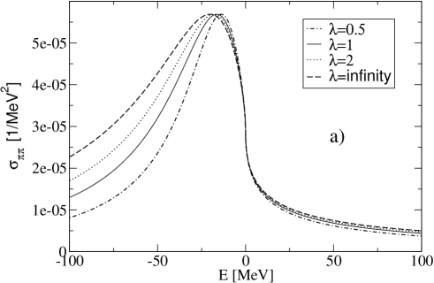
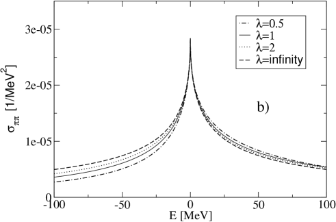
Figure 1: $\pi\pi$ cross section for different scaling parameters $\lambda$. The results are based on the Flatté parameters $R=4.76$, $\bar{g}_{\pi}$ = 0.317, $\bar{g}_{K}$ = 1.51, and $|E_{BW}|$ = 163.7 MeV of Ref. CMD2 . a) $E_{BW}<0$ , b) $E_{BW}>0$.

In order to illustrate the effect of the scale transformation we give, in Figs. 1, some examples of differential mass distributions in the scaling limit (6) and for different values of the parameter $\lambda$. The starting parameters $\Gamma_{P}$, $\bar{g}_{K}$ and $E_{BW}$ are those of Ref. CMD2 , given in Table 2.Fig. 1a shows the results for negative $E_{BW}$ and Fig. 1b those for positive $E_{BW}$. One can see that scaling is practically fulfilled for the energy interval of roughly $\pm$ 25 MeV around the $K\bar{K}$ threshold. Indeed, the cross sections above the threshold are basically the same for all $\lambda$ up to the highest considered excess energy of 100 MeV. For energies below the threshold and $E_{BW}<$ 0 scaling breaks down soon and there are already significant differences in the cross sections for energies around $E\approx-50$ MeV, whereas for the case of $E_{BW}>$ 0 those differences remain small down to even -100 MeV.

Of course, the range of scaling depends to some extent on the parameters $R$ and $\alpha$. In order to demonstrate this we show, in Fig. 2, results obtained with the parameters of Ref. Bugg . Here the ratio $R$ is more than three times smaller than for the case considered above. It is clear from Fig. 2 that the scaling behaviour is practically limited to the region very near to the $K\bar{K}$ threshold when the ratio $R$ is relatively small.

Since the shape of the mass distribution near the $K\bar{K}$-threshold is scale-invariant, as we just found, it is interesting to discuss what happens with the position of the singularities of the amplitude (2) as a function of the scaling parameter $\lambda$. The position of the poles in the complex $k$-plane can be given in terms of the $K\bar{K}$ scattering length $a$ and effective range $r_{e}$:

$$k_{1,2}=\frac{i}{r_{e}}\pm\sqrt{-\frac{1}{r_{e}^{2}}+\frac{2}{ar_{e}}}\ .$$ (10)

Those effective range parameters can then be related to the Flatté parameters $E_{BW}$, $\Gamma_{P}$ and $\bar{g}_{K}$:

$$a=-\frac{\bar{g}_{K}}{2(E_{BW}-i\Gamma_{P}/2)},~{}~{}r_{e}=-\frac{4}{m\bar{g}_{K}}.$$ (11)

Note that in the Flatté parametrization of the scattering amplitude the effective range is always negative. This is in contradiction to the usual interpretation of the effective range as interaction range xxx , which should be positive of course. We should mention, however, that in the case of potential models the effective range can be positive as well as negative (see, e.g., Ref. yyy ). A positive effective range can be also obtained if one takes into account the so-called finite width corrections as it is done in the Flatté-like distribution of Achasov, cf. the Appendix and also the work of Kerbikov Kerbikov .

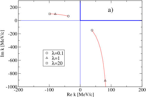
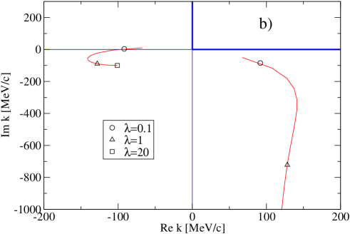
Figure 3: Trajectories of the poles in the complex $k$-plane, where $k$ is the cms momentum in the $K\bar{K}$ system. The same Flatté parameters as in Fig. 1 are used. The scaling parameters $\lambda$ is varied. a) $E_{BW}<0$ , b) $E_{BW}>0$. The physical region of the variable $k$ is indicated by the thick solid lines.

As is seen from Eqs. (11) the scattering length $a$ remains unchanged by the scale transformation (8) whereas the effective range $r_{e}$ rescales according to $r_{e}\to r_{e}/\lambda$. From Eq. (10) we conclude that in the limit of small $\lambda$ both roots are located near the points $k=\pm\sqrt{2/ar_{e}}$, i.e. practically symmetric around the point $k=0$. This corresponds to the case where the pure BW resonance dominates the cross section. In the limit of large $\lambda$ the effective range is getting small and the nearest pole to the point $k=0$ is located at $k_{1}\approx 1/a$. The second pole is at $k_{2}=2i\lambda/r_{e}$ and plays practically no role anymore for the physics around the $K\bar{K}$ threshold. In Figs. 3 we show the trajectories of the poles of the scattering amplitudes (9) as a function of the parameter $\lambda~{}~{}(0.1\leq\lambda<\infty)$ for the same sets of parameters ($\bar{g}_{P},\bar{g}_{K},E_{BW}$) used for the results in Figs. 1.

The limiting, scale-invariant form of the cross section as given by the Eqs. (6) corresponds to the scattering amplitude in the zero range approximation, i.e. to

$$f_{el}=\frac{1}{R}~{}\frac{1}{-a^{-1}-ik}\ .$$ (12)

The scattering length $a$ can be expressed in terms of the ratios $R$ and $\alpha$ and the relative momentum of the light particles at the $K\bar{K}$ threshold, $q_{th}$:

$$a=-\frac{1}{q_{th}}\frac{R}{\alpha-i}\ .$$ (13)

Thus, since the ratios $R$ and $\alpha$ can be extracted from a study of the near-threshold momentum dependence of the invariant mass spectrum, a determination of the (complex) $K\bar{K}$ scattering length is also feasible.

3 Resonance - threshold interplay: poles, cross sections and phase shifts

In a previous paper evidence we discussed the concept of “pole counting” suggested by Morgan morgan as a tool for near-threshold resonance classification. It was demonstrated that the existence of a pair of poles in the complex $k$-plane in the vicinity of the threshold of the heavy particles corresponds to the situation where a resonance has a large admixture of an elementary (bare) state made up of a quark-antiquark pair, say. In contrary the situation when there is only one pole near the threshold point $k=0$ corresponds to the molecule-like picture of a resonance.

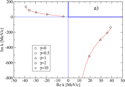
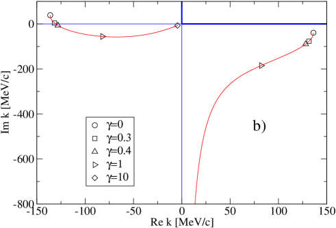
Figure 4: Trajectories of the poles in the complex $k$-plane, where $k$ is the cms momentum in the $K\bar{K}$ system. The results are based on the Flatté parameters $\bar{g}_{\pi}$ = 0.09, $\bar{g}_{K}$ = 0.97, and $|E_{BW}|$ = 34.3 MeV of Ref. OPAL . The coupling strength to the $K\bar{K}$ channel is varied by $\gamma\times\bar{g}_{K}$. a) $E_{BW}<0$ , b) $E_{BW}>0$. The physical region of the variable $k$ is indicated by the thick solid lines.

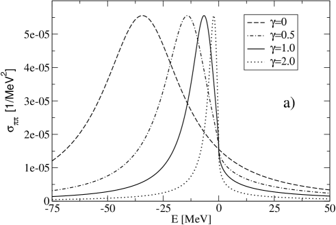
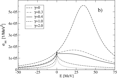
Figure 5: Results for the $\pi\pi$ cross section. The same Flatté parameters as in Fig. 4 are used. The coupling strength to the $K\bar{K}$ channel is varied by $\gamma\times\bar{g}_{K}$. a) $E_{BW}<0$, b) $E_{BW}>0$.

The role of the $K\bar{K}$ threshold for the shape of the differential mass spectra becomes more transparent if one studies the pole positions in the $k$-plane as a function of the strength of the coupling to the $K\bar{K}$ channel, $\bar{g}_{K}$, while keeping the other two parameters, $E_{BW}$ and $\Gamma_{P}$, fixed. Corresponding results are presented in Fig. 4. In parallel we also look at the behaviour of the elastic cross section in the channel of the light particles. Those results are shown in Figs. 5. As an example we take the Flatté parameters of Ref. OPAL , given in Table 2, as starting point. The coupling strength $\bar{g}_{K}$ is varied by multiplying it with a factor $\gamma$ and we label the corresponding curves in the figures with the values chosen for $\gamma$.

In the $k$-plane the position of the poles is given by Eq. (10). Note, that in the limit $\bar{g}_{K}\to 0$ we get $a\to 0$ and $r_{e}\to-\infty$, see Eq. (11). However, combining Eqs. (10) and (11) we see that in the limit $\bar{g}_{K}\to 0$ the poles of the amplitude (2) are at $k_{1,2}=\pm\sqrt{2/ar_{e}}=\pm\sqrt{m_{K}(E_{BW}-i\Gamma_{P}/2)}$. These are simply the poles of the pure BW amplitude. They are located in the 2nd and 4th quadrants of the $k$-plane and they are symmetric with respect to the point $k=0$, cf. Fig. 4. Note that in the limit $\bar{g}_{K}\to 0$ the resonance is completely decoupled from the $K\bar{K}$ system. The proximity of the resonance state to the $K\bar{K}$ threshold is then just accidental.

The elastic cross sections corresponding to the uncoupled case are shown as dashed lines in Fig. 5. For $E_{BW}<0$ (Fig. 5a) the resonance is located below the $K\bar{K}$ threshold. Note that in this case the pole from the 2nd quadrant is closer to the physical region of the variable $k$ (the physical region of the variable $k$ is indicated by the thick solid lines in Figs. 4a,b) and causes the structure in the cross section. For $E_{BW}>0$ (Fig. 5b) the resonance manifests itself as a bump in the cross section at energies above the $K\bar{K}$ threshold. In this case the pole in the 4th quadrant is located closer to the physical region and is responsible for the structure in the cross section.

When the coupling to the $K\bar{K}$ channel is switched on and $\bar{g}_{K}$ increases, the position of both poles begins moving downwards in the (complex) $k$-plane for $E_{BW}>0$ and also for $E_{BW}<0$, cf. Fig. 4. For very large values of $\bar{g}_{K}$ the pole, located initially in the 2nd quadrant, moves to the limiting point $k=0$ and the second pole moves to $-i\infty$. In this case, according to Eq. (11), the scattering length $a$ goes to infinity and the effective range $r_{e}$ goes to zero. In the regime of large coupling, $\bar{g}_{K}\gg\bar{g}_{\pi}$, we have only one pole near the point $k=0$ and the approximate expression for elastic scattering amplitude is given again by Eq. (12). This situation corresponds to a molecule-like structure of the near threshold resonance evidence . Note that most of the available Flatté parametrizations indicate that the scenario of $\bar{g}_{K}\gg\bar{g}_{\pi}$ is roughly fulfilled for the $f_{0}(980)$ case, cf. Table 2. In this context let us emphasize that $\bar{g}_{K}\gg\bar{g}_{\pi}$ corresponds to a large ratio $R$. The latter quantity can be extracted fairly reliably from Flatté parametrizations of the experimental invariant mass distribution as we showed in the last section.

The corresponding evolution of the cross section with increasing of the coupling strength can be seen from Figs. 5. For $E_{BW}<0$ the initial pure BW resonance evolves into a distinct structure that approaches the $K\bar{K}$ threshold when the channel coupling is switched on and gradually increased. The maximum of the cross section remains always below the threshold. Clearly, the pole, which is responsible for the structure in the cross section for small values of $\bar{g}_{K}$ and which was located in the 2nd quadrant, retains its influence on the resonance shape for all values of $\bar{g}_{K}$ whereas the second pole (in the 4th quadrant) is not significant. For the case $E_{BW}>0$ (Fig. 5b) we see again the developement of a distinct structure in the cross section which, however, is now a cusp located exactly at the $K\bar{K}$ threshold. Also the general situation is different. As already said, for small values of $\bar{g}_{K}$ the pole located in the 4th quadrant is closer to the physical region and is responsible for the structure in the cross section. With increasing $\bar{g}_{K}$ this pole moves away from the physical region. Simultaneously the pole from the 2nd quadrant moves closer to the physical region and takes over the dominant role. Thus we observe here that, with increasing $\bar{g}_{K}$, one leading pole is substituted by another!

In this context it is interesting to look also at the behaviour of the corresponding phase shifts. The $S$-matrix corresponding to the Flatté amplitude (2) is given by

$$S=\eta\exp{(2i\delta(k))}=\frac{E-E_{BW}-i\Gamma_{P}/2+i\bar{g}_{K}k/2}{E-E_{BW}+i\Gamma_{P}/2+i\bar{g}_{K}k/2}\ .$$ (14)

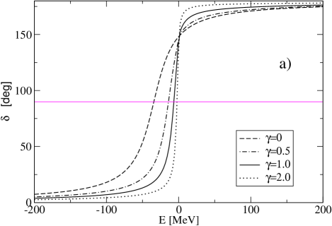
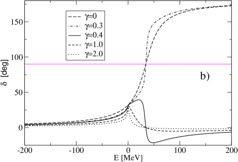
Figure 6: $\pi\pi$ phase shift $\delta$ in the $J=0$, $I=0$ partial wave. The same Flatté parameters as in Fig. 4 are used. The coupling strength to the $K\bar{K}$ channel is varied by $\gamma\times\bar{g}_{K}$. a) $E_{BW}<0$, b) $E_{BW}>0$

Phase shifts $\delta(k)$ for fixed $|E_{BW}|$ and $\Gamma_{P}$ and several values of the coupling constant $\bar{g}_{K}$ are presented in Figs. 6. The long dashed lines are the results for the uncoupled situation, i.e. for $\bar{g}_{K}$ = 0. In this case the phase shifts go through $90^{\circ}$ at the nominal BW resonance energy $E_{BW}$. When the coupling to the $K\bar{K}$ channel is switched on and increased there is a significant difference in the developement of the phases for $E_{BW}<0$ and $E_{BW}>0$. For $E_{BW}<0$ (Fig. 6a) the energy where the phase passes through $90^{\circ}$ moves closer and closer to the threshold and at the same time the rise of the phase is getting steeper and steeper. Thus, for a strong coupling to the $K\bar{K}$ channel (i.e. a large $\bar{g}_{K}$) the behaviour of the phase shift is completely dominated by the occurence of the threshold. The parameter values of the initial BW resonance ($E_{BW}$ and $\Gamma_{P}$) play practically no role anymore.

The results for $E_{BW}>0$ are shown in Fig. 6b. As can be seen, for small coupling ($\bar{g}_{K}\leq 0.3$) the phase shifts increase from $0^{\circ}$ to $180^{\circ}$ with increasing energy – whereby a more and more pronounced kink develops at the $K\bar{K}$ threshold. At a certain value of $\bar{g}_{K}$ there is suddenly a jump in the phase and from there onwards the phase always approaches zero for increasing energy! This specific behaviour of the phase for $E_{BW}>0$ may be understood by looking at the trajectories of the poles, shown in Fig. 4b. For $\bar{g}_{K}=0$ we have a pair of poles located symmetric with respect to the point $k=0$ and the pole in the 4th quadrant is nearest to the physical region of the variable $k$. When $\bar{g}_{K}$ increases both poles move down in the complex plane. Then, at some stage, the pole located initially in the 2nd quadrant, crosses the real axis of the $k$-plane and reaches the 3rd quadrant. (In the specific case shown this occurs for $\bar{g}_{K}\approx 0.33$.) In the absence of absorption (i.e. for $\Gamma_{P}=0$) this transition corresponds to the mutation of a real bound state (in the $K\bar{K}$ system) to a virtual state. This change is reflected also in the $\pi\pi$ system, namely by the mentioned jump in the phase shift. In case of $E_{BW}<0$, the second pole remains in the upper half-plane for all values of $\bar{g}_{K}$, see Fig. 4a. In this case a bound state exists for all values of $\bar{g}_{K}$ and the global features of the phase do not change.

4 The $f_{0}$ and $a_{0}$ mesons

Let us first discuss the $f_{0}(980)$ resonance. Here the relevant $S$-wave $\pi\pi$ phase shift in the isospin $I=0$ channel is known experimentally over a wide energy range, see, e.g. Refs. Hyams ; Protopopescu ; Hyams1 ; bnl and also the more recent analyses in Refs. KLR02 ; Achasov03 . The situation for the $f_{0}(980)$ resonance differs significantly from the ideal situation where there is no background, which was discussed in Sections 2 and 3, because the phase shift exhibits already a nontrivial behaviour below the $f_{0}(980)$ region. It rises monotonously from the $\pi\pi$ threshold onwards and reaches $90^{o}$ already at an energy around $700$ MeV. Usually this behaviour is explained via the presence of a broad scalar resonance called $\sigma$ or $f_{0}(400-1200)$ PDG which is believed to be a pure rescattering effect, see, e.g., Ulf . This broad resonance provides the background for the $f_{0}(980)$ meson. Because of this large background the $f_{0}(980)$ meson manifests itself as a narrow dip located near the $K\bar{K}$-threshold in some production reactions rather than as a bump Sassen .

Still, because the $\pi\pi$ $S$-wave phase shift is known experimentally, at least at a first glance the chances for a determination of the resonance parameters appear to be much more promising for the channel with isospin $I=0$ than for the one with $I=1$ (i.e. for the case of the $a_{0}$ meson). Specifically, one would hope that the knowledge of the $S$-wave phase shift allows to fix the scale of the coupling constants $\bar{g}_{\pi}$ and $\bar{g}_{K}$ for the $f_{0}$ case. Unfortunately, in practice the situation is much more complicated. The main problem is, of course, that experimentally only the total phase shift can be extracted, and the phase of the background can not be disentangled unambiguously from the contribution of the $f_{0}$ resonance. Thus, by making different assumptions about the behaviour of the background one will always get different solutions for parameters of the $f_{0}$ resonance. The second difficulty is that each of the phase shift analyses is afflicted by fairly large error bars. In addition, there are also drastic differences between the results of some of those phase shift analyses (compare, e.g., Refs. Hyams ; Protopopescu ; Hyams1 ; bnl ; KLR02 ; Achasov03 ) for $\pi\pi$ scattering. These differences preclude the possibility to extract a uniqiue set of parameters for the $f_{0}(980)$ resonance.

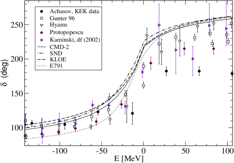
Figure 7: $\pi\pi$ phase shift $\delta$ in the $J=0$, $I=0$ partial wave. The curves are results based on Flatté distributions taken from Refs. SND ; CMD2 ; KLOE ; E791 . The symbols show results from various phase shift analyses taken from Refs. Hyams ; Protopopescu ; bnl ; KLR02 ; Achasov03 .

To illustrate the two above remarks, we show in Fig. 7 the experimental phases taken from Refs. Hyams ; Protopopescu ; bnl ; KLR02 ; Achasov03 . We also present the $\pi\pi$ phases reconstructed from the parameters for the $f_{0}$ meson obtained from different analyses SND ; CMD2 ; KLOE ; E791 . The latter results exemplify that all parameter sets, and in particular those from radiative $\phi$-decays, yield very similar phase shifts, despite of the fact that the parameters of the $f_{0}(980)$ resonance differ drastically (see Table 2). Thus, they exhibit the typical scaling behaviour that we discussed above. Note that for those curves we have added a background phase which grows smoothly from 70^o to 90^o in the energy region 150 MeV around threshold. We did this in order to enable a direct comparison of the calculated results with the energy dependence of the experimental phase shifts. In all shown cases the same background phase is used.

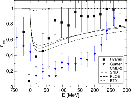
Figure 8: Inelasticity in the $\pi\pi$ $J=0$, $I=0$ partial wave. The curves are results based on Flatté parameters taken from Refs. SND ; CMD2 ; KLOE ; E791 . The symbols show results from phase shift analyses taken from Refs. Hyams ; bnl .

The sensitivity of the inelasticity $\eta$ (the definition of $\eta$ is given by Eq. (14)) to the Flatté parameters is demonstrated in Fig. 8 for the case of the $f_{0}(980)$ meson. Experimental data for the $S$-wave $I=0$ $\pi\pi$ inelasticities are taken from Refs. Hyams ; bnl . Though there are some variations in the results of different parametrizations it is obvious that todays experimental knowledge of the inelasticity in $\pi\pi$ scattering near threshold is not sufficient for determining the parameters for the $f_{0}$ resonance.

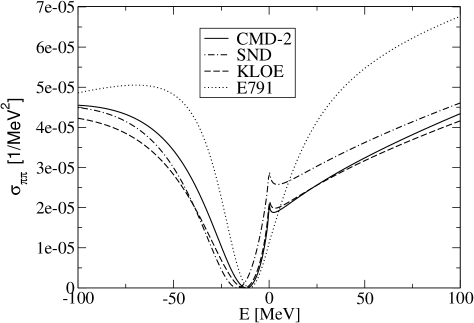
Figure 9: Results for the $\pi\pi$ cross section. The curves are results based on Flatté distributions taken from the Refs. SND ; CMD2 ; KLOE ; E791 .

Results for the $\pi\pi$ elastic cross section based on those Flatté parametrizations are shown in Fig. 9. We can see again that most of those parametrizations yield rather similar predictions.

Now let us discuss shortly the $a_{0}$ meson. As is seen from Tables 1 and 2 the strength of the coupling to the $K\bar{K}$-channel, $\bar{g}_{K}$, is much weaker for the $a_{0}$ meson, than for the $f_{0}$ meson whereas the coupling to the $\pi\pi$ or $\pi\eta$ channels is comparable. Accordingly, the ratio $R$ is, in general, significantly smaller for the $a_{0}$ case. As a consequence, for the $a_{0}$ meson the magnitude of the effective range is much larger and both singularities of the scattering amplitude influence the differential cross section near the $K\bar{K}$ threshold. These aspects were already discussed in our previous paper evidence .

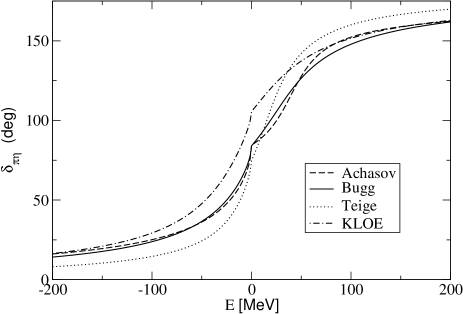
Figure 10: $\pi\eta$ phase shift $\delta$ in the $J=0$, $I=1$ partial wave. The curves are results based on Flatté distributions taken from Refs. Teige ; Bugg ; KLOEa ; AchKi .

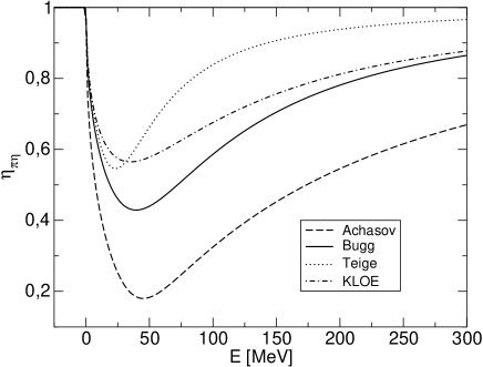
Figure 11: Inelasticity in the $\pi\eta$ $J=0$, $I=1$ partial wave. The curves are results based on Flatté parameters taken from Refs. Teige ; Bugg ; KLOEa ; AchKi .

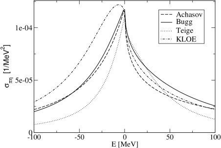
Figure 12: Total cross section in the $\pi\eta$ $J=0$, $I=1$ partial wave. The curves are results based on Flatté parameters taken from Refs. Teige ; Bugg ; KLOEa ; AchKi .

The behaviour of the $\pi\eta$ $S$-wave phase shift is presented in Fig. 10 for the Flatté parametrizations given in Refs. Teige ; Bugg ; KLOEa ; AchKi . Also here one sees that there is basically no difference in the prediction for the phase shifts despite the fact that all sets of parameters are quite different. However, the situation is somewhat different for the $\pi\eta$ inelasticity $\eta$ which is shown in Fig. 11 and also for the $\pi\eta$ total cross section (cf. Fig. 12). Here there are stronger variations between the results produced by the different parametrizations. Thus, the scaling behavior is not so pronounced for the case of the $a_{0}$ meson, which could be already guessed from the smaller ratio $R$ (cf. discussion in section 2). Consequently, for the $a_{0}$ resonance there could be a better chance to determine all three Flatté parameters as compared to the $f_{0}$ meson.

These examples show that the determination of the “true” values for the parameters of the $a_{0}$ as well as the $f_{0}$ meson is a rather challenging problem. It requires, first of all, a very significant improvement in the accuracy of the experimental data.

5 Conclusions

In the present paper we studied properties of the Flatté amplitude (2), which is usually employed to describe differential mass distributions resulting from $S$-wave resonance like structures, located near a threshold. Specifically, such Flatté and Flatté-like distributions are often used to describe and derive properties of the scalar mesons $a_{0}(980)$ and $f_{0}(980)$. But there are also some other examples of hadronic resonances, located near thresholds, where it is reasonable to represent them in terms of the Flatté distribution.

The Flatté parametrization of the amplitude includes three free parameters which should be determined from the experimental mass spectrum. These are the nominal mass of the resonance, $m_{R}$, the inelastic width at threshold, $\Gamma_{P}$, (or the coupling constant for the channel of the light particles, $\bar{g}_{P}$), where $P$ stands for $\pi\pi$ or $\pi\eta$, and the coupling constant $\bar{g}_{K}$ for the channel of the heavy particles.

We showed that the mass spectrum near threshold is not sensitive to all the parameters ($E_{BW}$, $\bar{g}_{P}$, $\bar{g}_{K}$) but rather only to the two dimensionless ratios $R=\bar{g}_{K}/\bar{g}_{P}$ and $\alpha=2E_{BW}/\Gamma_{P}$. Those are the two parameters that determine also the scattering length in the channel with the heavy particles. This difficulty of fixing all three Flatté parameters concerns the standard Flatté distribution but also relativistic extensions like the one proposed by Achasov and is clearly reflected in the parameter values for the $a_{0}$(980) and $f_{0}$(980) mesons that can be found in the literature (cf. Tables 1 and 2). The results of those fits to the data exemplify that there is a large uncertainty in the absolute values of the coupling constants, whereas the ratios $R$ and $\alpha$ can be extracted from experiments with much better accuracy.

In principle, only the information about the absolute values of the coupling constants and the nominal resonance mass opens the possibility to calculate the $K\bar{K}$ effective range parameters and to reconstruct the position of the poles of the scattering amplitude in the complex $k$-plane. As was stressed in Ref. evidence and in line with the suggestion made by Morgan morgan , the knowledge of the position of the poles of the scattering amplitude allows to draw conclusions on the nature of the resonance, i.e. to clarify, whether it corresponds to an elementary object made from quarks or whether it is a compound state like a $K\bar{K}$ molecule. However, the ratio $R$ of the coupling constants is an interesting quantity too. For example, a large $R$, i.e. a large coupling to the $K\bar{K}$ channel is a strong indication for a molecular-like structure of the near-threshold resonance. Fortunately, as we have shown, this ratio can be determined from a Flatté parametrization of the mass distributions with significantly better reliability than the absolute values of the coupling constants.

6 Appendix

The elastic scattering amplitude for the channel with the light particles for the relativistic Flatté distribution has the form

$$f_{el}=-\frac{1}{q}\,\frac{\Gamma_{P}m_{R}}{m^{2}-m_{R}^{2}+im_{R}(\Gamma_{P}+\bar{g}_{k}\frac{k}{2})}\ .$$ (15)

In the nonrelativistic limit it can be rewritten as

$$f_{el}=-\frac{1}{2q}\frac{\Gamma_{P}}{E-E_{BW}+i\frac{\Gamma_{P}}{2}+i\bar{g}_{K}\frac{k}{2}}\ .$$ (16)

where we used the notation introduced in Section 2.

Let us demonstrate in this Appendix that the relativistic Flatté-like distribution introduced by Achasov AchKi , i.e. the expression

$$f_{el}=-\frac{1}{q}\,\frac{\Gamma_{P}m_{R}}{m^{2}-m_{R}^{2}+\sum_{ab}[\rm\Pi^{ab}(m^{2})-Re\Pi^{ab}(m_{R}^{2})]},$$ (17)

where $\rm\Pi$ takes into account the so called finite width corrections to the self-energy loop of the resonance with nominal mass $m_{R}$ from the two-particle intermediate states $ab$ ($\pi\pi$ or $\pi\eta$ and $K\bar{K}$), reduces to the form given in Eq. (16) in the nonrelativistic limit. In the region $m\geq m_{a}+m_{b}$ the expression for $\rm\Pi^{ab}$ is

$$\Pi^{ab}(m^{2})=\frac{g^{2}_{ab}}{16\pi}\left[\frac{m_{+}m_{-}}{\pi m^{2}}\ln\frac{m_{b}}{m_{a}}+\right.$$

$$\left.+\rho_{ab}\left(i+\frac{1}{\pi}\ln\frac{\sqrt{m^{2}-m_{-}^{2}}-\sqrt{m^{2}-m_{+}^{2}}}{\sqrt{m^{2}-m_{-}^{2}}+\sqrt{m^{2}-m_{+}^{2}}}\right)\right],$$ (18)

where $m_{\pm}=m_{a}\pm m_{b}$ with $m_{a}\geq m_{b}$ and
$\rho_{ab}(m)=\sqrt{(1-\frac{m_{+}^{2}}{m^{2}})(1-\frac{m_{-}^{2}}{m^{2}})}\,$. In the nonrelativistic limit the expressions for $\Delta{\rm\Pi}^{ab}/4m_{K}=\left[{\rm Re\>\Pi}^{ab}(m^{2})-{\rm Re\>\Pi}^{ab}(m_{R}^{2})\right]/4m_{K}$ take the form

$$\frac{\Delta\>{\rm\Pi}^{K\bar{K}}}{4m_{K}}\approx\frac{\bar{g}_{K}}{\pi}(E-E_{R})$$

$$\frac{\Delta\>{\rm\Pi}^{P}}{4m_{K}}=\frac{\bar{g}_{P}}{4\pi}(E-E_{R})\>C_{P}$$ (19)

where $P$ denotes $\pi\pi$ or $\pi\eta$ loops and

$$C_{P}=\left\{\frac{m_{+}m_{-}}{2m_{k}^{2}}\ln\frac{m_{b}}{m_{a}}\right.$$

$$\left.-A_{-}A_{+}\left[(B_{-}+B_{+})\ln\frac{A_{-}-A_{+}}{A_{-}+A_{+}}+\frac{A_{-}A_{+}(B_{-}-B_{+})}{A_{-}^{2}-A_{+}^{2}}\right]\right\},$$ (20)

$$A_{\pm}=\sqrt{1-\frac{(m_{a}\pm m_{b})^{2}}{4m_{K}^{2}}},\>B_{\pm}=\frac{(m_{a}\pm m_{b})^{2}}{4m_{K}^{2}-(m_{a}\pm m_{b})^{2}}.$$ (21)

Note that the expression for $C_{\pi\pi}$ can be easily simplified to

$$C_{\pi\pi}=2\left(1-\frac{m_{\pi}^{2}}{m_{K}^{2}}\ln\frac{m_{\pi}}{2m_{K}}\right)+O\left(\frac{m_{\pi}^{2}}{m_{K}^{2}}\right)\approx 2.32,$$ (22)

whereas the evalution of $C_{\pi\eta}$ gives the value 2.81.

Thus, using the nonrelativistic expansion of the loop corrections (Eqs.19) Eq.(17) can be reduced to the standard Flatté form. For example, for the $f_{0}$ meson, one gets

$$f_{\pi\pi}=-\!\frac{1}{2q}\times$$ (23)

$$\frac{\Gamma_{P}}{(E\!-\!E_{R})(1\!-\!\frac{\bar{g}_{K}}{\pi}\!-\!\frac{\bar{g}_{\pi}}{4\pi}C_{\pi\pi})\!+\!\frac{\bar{g}_{K}}{2}\sqrt{m|E_{R}|}\Theta(\!-E_{R})+i\frac{\Gamma_{P}}{2}+i\bar{g}_{K}\frac{k}{2}}$$

$$= -\frac{1}{2q}\,\frac{\tilde{\Gamma}_{P}}{E\!-E_{BW}\!+\!i\frac{\tilde{\Gamma}_{P}}{2}\!+\!i\tilde{g}_{K}\frac{k}{2}},$$

where

$$\tilde{g}_{\pi}=\frac{\bar{g}_{\pi}}{1-\displaystyle\frac{\bar{g}_{K}}{\pi}-\frac{\bar{g}_{\pi}}{4\pi}C_{\pi\pi}},\ \tilde{g}_{K}=\frac{\bar{g}_{K}}{1-\displaystyle\frac{\bar{g}_{K}}{\pi}-\displaystyle\frac{\bar{g}_{\pi}}{4\pi}C_{\pi\pi}},$$

$$\tilde{\Gamma}_{P}=\tilde{g}_{\pi}q,$$ (24)

$$E_{BW}=\!E_{R}\!-\!\displaystyle\frac{\tilde{g}_{K}}{2}\sqrt{m|E_{R}|}\Theta(-E_{R}),$$ (25)

$$\alpha=\frac{2E_{BW}}{\tilde{\Gamma}_{P}}\ .$$ (26)

Note that the term $\displaystyle\frac{\bar{g}_{K}}{2}\sqrt{m|E_{R}|}\Theta(-E_{R})$ in the denominator results from the piece $\rm Re\Pi(m_{R}^{2})$ in the case of a negative $E_{R}$. We want to mention also that for some values of the parameters $\bar{g}_{K}$ and $\bar{g}_{\pi}$ the expression ${1-\displaystyle\frac{\bar{g}_{K}}{\pi}-\frac{\bar{g}_{\pi}}{4\pi}C_{\pi\pi}}$ can change the sign. In this case the effective range in Eq. (11) also changes its sign and becomes positive. Then the relativistic distribution introduced by Achasov (Eq. (17)) no longer can be reduced to the standard nonrelativistc form (16) but it will go over into what one might call an Anti-Flatté distribution, i.e. into a form that is identical to Eq. (16) but where the sign of the real part in the denominator is reversed.

Figure 2: $\pi\eta$ cross section for different scaling parameters $\lambda$. The results are based on the Flatté parameters $R=1.14$, $\bar{g}_{\pi}$ = 0.454, $\bar{g}_{K}$ = 0.506, and $E_{BW}$ = 7.6 MeV of Ref. Bugg .

References

- (1) D. V. Bugg, Phys. Rept. 397, 257 (2004).
- (2) E. Klempt, hep-ph/0404270.
- (3) F.E. Close and N.A. Tornqvist, J. Phys. G 28, R249 (2002); C. Amsler and N.A. Tornqvist, Phys. Rept. 389, 61 (2004).
- (4) J.A. Oller, E. Oset , and A. Ramos, Prog. Part. Nucl. Phys. 45, 157 (2000).
- (5) E. van Beveren and G. Rupp, hep-ph/0406242.
- (6) V.V. Anisovich, Phys. Usp. 47, 45 (2004) [Usp. Fiz. Nauk 47, 49 (2004)]; arXiv:hep-ph/0208123.
- (7) S. Flatté, Phys. Lett. 63B, 224 (1976).
- (8) S. Teige et al., Phys. Rev. D 59, 012001 (1999).
- (9) D.V. Bugg, V.V. Anisovich, A. Sarantsev, and B.S. Zou, Phys. Rev. D 50, 4412 (1994).
- (10) A. Abele et al., Phys. Rev. D 57, 3860 (1998).
- (11) M.N. Achasov et al., Phys. Lett. B479, 53 (2000).
- (12) A. Aloisio et al., Phys. Lett. B536, 209 (2002).
- (13) N.N. Achasov and A.N. Kisilev, Phys. Rev. D 68, 014006 (2003).
- (14) M.N. Achasov et al., Phys. Lett. B485, 349 (2002).
- (15) R.R. Akhmetshin et al., Phys. Lett. B462, 380 (1999).
- (16) A. Aloisio et al., Phys. Lett. B537, 21 (2002); A. Antonelli, hep-ex/0209069 (2002).
- (17) E. M. Aitala et al. [E791 Collaboration], Phys. Rev. Lett. 86, 765 (2001).
- (18) D. Barberis et al. [WA102 Collaboration], Phys. Lett. B 462, 462 (1999).
- (19) K. Ackerstaff et al. [OPAL Collaboration], Eur. Phys. J. C 4, 19 (1998).
- (20) N.N. Achasov and V.V. Gubin, Phys. Rev. D 63, 094001 (2001).
- (21) see, e.g., R.G. Newton, Scattering Theory of Waves and Particles, (Springer-Verlag, New York, 1982).
- (22) M.M. Nagels, T.A. Rijken, and J.J. de Swart, Phys. Rev. D 20, 1633 (1979); B. Holzenkamp, K. Holinde, and J. Speth, Nucl. Phys. A500, 485 (1989).
- (23) B. Kerbikov, hep-ph/0402022.
- (24) V. Baru, J. Haidenbauer, C. Hanhart, Yu.S. Kalashnikova, and A. Kudryavtsev, Phys. Lett. B 586, 53 (2004); Yu.S. Kalashnikova, arXiv:hep-ph/0311302.
- (25) D. Morgan, Nucl. Phys. A543, 632 (1992).
- (26) B. Hyams et al., Nucl. Phys. B 64, 134 (1973) [AIP Conf. Proc. 13, 206 (1973)].
- (27) S. D. Protopopescu et al., Phys. Rev. D 7, 1279 (1973).
- (28) B. Hyams et al., Nucl. Phys. B100, 205 (1975).
- (29) J. Gunter et al. [E852 Collaboration], arXiv:hep-ex/9609010.
- (30) R. Kaminski, L. Lesniak and K. Rybicki, Eur. Phys. J. directC 4, 4 (2002) [arXiv:hep-ph/0109268].
- (31) N. N. Achasov and G. N. Shestakov, Phys. Rev. D 67, 114018 (2003).
- (32) K. Hagiwara et al., Phys. Rev. D 66, 010001 (2002).
- (33) U.-G. Meißner, Comm. Nucl. Part. Phys. 20, 119 (1991).
- (34) F.P. Sassen, S. Krewald, and J. Speth, Eur. Phys. J. A 18, 197 (2003).