Some aspects of $\Theta^{+}$ parity determination in the reaction $\gamma\,N\to\Theta^{+}\,\bar{K}\to N\,K\bar{K}$

Abstract

We analyze the problem of how to determine the parity of the $\Theta^{+}$ pentaquark in the reaction $\gamma N\to K\Theta\to NK\bar{K}$, where $N=n,p$. Our model calculations indicate that the contribution of the non-resonant background of the reaction $\gamma N\to NK\bar{K}$ cannot be neglected, and that suggestions to determine the parity based solely on the initial-stage process $\gamma N\to K\Theta$ cannot be implemented cleanly. We discuss the various mechanisms that contribute to the background, and we identify some spin observables which are sensitive mostly to the $\Theta^{+}$ parity rather than to the details of the production mechanism.

I Introduction

The first evidence for the $\Theta^{+}$ pentaquark discovered by the LEPS collaboration at SPring-8 Nakano03 was subsequently confirmed in other experiments DIANA ; CLAS1 ; CLAS2 ; SAPHIR03 ; Asratyan ; NOMAD . None of these experiments could determine the spin and the parity of the $\Theta^{+}$. Some proposals to do this in photoproduction processes using single and double polarization observables were discussed in Refs. NT03 ; Zhao03 ; ZhaoKhal04 . The difficulty in determining the spin and parity of $\Theta^{+}$ in the reaction $\gamma N\to\Theta^{+}K^{-}$ is due to the way the pentaquark state is produced. The models of the $\Theta^{+}$ photoproduction from the nucleon based on the effective Lagrangian approach have been developed in Refs. Hosaka03 ; OKL031 ; NT03 ; LiuKo031 ; LiuKo032 ; LiuKo033 ; Zhao03 ; ZhaoKhal04 ; Oh-2 ; CloseZhao . As has been pointed out, there are great ambiguities in calculating the (spin) unpolarized and polarized observables. In the effective Lagrangian formalism the problems are summarized as follows:

(1) Dependence on the coupling operator for the $\Theta^{+}NK$ interaction, i.e., whether one chooses pseudoscalar (PS) or pseudovector (PV) couplings. In the case of PV coupling, gauge invariance requires a Kroll-Ruderman-type contact term even for undressed particles which affects both unpolarized and polarized observables. For dressed particles, in a tree-level description, contact currents also are required for PS coupling.

(2) Ambiguity due to the choice of the coupling constants. At the simplest level, five unknown coupling constants and their phases enter the formalism: $g_{\Theta NK}$ in the $\Theta^{+}NK$ interaction; the vector and tensor couplings $g_{\Theta NK^{*}}$ and $\kappa^{*}$, respectively, in the $\Theta^{+}NK^{*}$ interaction, and the tensor coupling $\kappa_{\Theta}$ in the electromagnetic $\gamma\Theta^{+}$ interaction. To fix the absolute value of $g_{\Theta NK}$, one can use the relation between $g_{\Theta NK}$ and the $\Theta$ decay width $\Gamma_{\Theta}$. This provides, however, only an upper limit for $|g_{\Theta NK}|$ because all the experiments give only upper limits of the decay width (about 25 MeV) which are comparable with the experimental resolution.

(3) Dependence on the choice of the phenomenological form factors: (i) form factors suppress the individual channels in different ways, and (ii) form factors generate (modify) the contact terms for the PS (PV) coupling schemes which affect the theoretical predictions.

A possible solution to these problems is to use more complicated “model-independent” (triple) spin observables, discussed by Ejiri Ejiri , Rekalo and Tomassi-Gustafsson RT-G04 , and Nakayama and Love NL04 . These spin observables involve the linear polarization of the incoming photon, and the polarizations of the target nucleon and the outgoing $\Theta^{+}$. Using basic principles, such as the invariance of the transition amplitude under rotation, parity inversion and, in particular, the reflection symmetry with respect to the scattering plane, one can arrive at unambiguous predictions which depend only on the $\Theta^{+}$ parity in the reaction $\gamma N\to\Theta^{+}\bar{K}$. The key aspect of the model-independent predictions is that in the final state the total internal parity of outgoing particles are different for positive and negative $\Theta^{+}$ parity. We skip the discussions of the practical implementation of using the triple spin observables since experimental observations of the spin orientation of the strongly decaying $\Theta^{+}$ is extremely difficult. Instead, we focus on the basic aspects of this idea. For simplicity, in the following we limit our discussion for determining the $\Theta^{+}$ parity to isoscalar spin-1/2 $\Theta^{+}$. In fact, most theories predict the $J^{P}$ of $\Theta^{+}$ to be $1/2^{+}$ or $1/2^{-}$.

There are two difficulties in applying the “model-independent” formalism for the parity determination. First, the final state in the photoproduction experiment is the three-body state $NK\bar{K}$ (and not the two body $\Theta^{+}\bar{K}$)-state. The spin observables in the initial and final channels are deduced by their parities irrespective of the intermediate $\Theta^{+}$ parity. It is difficult, therefore, to find the pertinent “model-independent” observables for this case. Second, the contribution of the non-resonant background of the reaction $\gamma N\to NK\bar{K}$ cannot be neglected. The observed ratio of the resonance peak to the non-resonant continuum reported in the photoproduction experiments is about $1.5-2$. This means that the difference between the resonant and non-resonant amplitudes is a factor of two and therefore the non-resonant background may modify the spin-observables considerably.

The aim of the present paper is to discuss these important aspects. We show that strict predictions for the $\gamma N\to\Theta^{+}\bar{K}$ reactions lose their definiteness in the case of the $\gamma N\to NK\bar{K}$ processes, where $\Theta^{+}$ decays strongly into $NK$; they become model-dependent. Nevertheless, we try to identify the kinematic regions where this dependence is weak and a clear difference is expected for different $\Theta^{+}$ parities. In the following discussion, the term “resonant” is applied to processes which proceed through the virtual $\Theta^{+}$-state, whereas the term “non-resonant” is used for all other processes. The latter may have intermediate non-exotic resonant states as well. The resonant amplitude consists of $s$-, $u$-, $t$-channel terms and the contact ($c$) term defined by the $\Theta^{+}NK$ interaction, as depicted in Fig. 2a-d. We also have a $t$-channel $K^{*}$ exchange as shown in Fig. 2e. We found that the main contribution to the “non-resonant” background comes from the virtual vector-meson photoproduction $\gamma N\to VN\to NK\bar{K}$, depicted in Fig. 2a-c. We also have the excitation of the virtual scalar ($\sigma$) and tensor ($f_{2},a_{2}$) mesons shown in Fig. 2d-f, respectively, and found that their contribution in the near-threshold region with $E_{\gamma}\approx 2$ GeV is negligible.

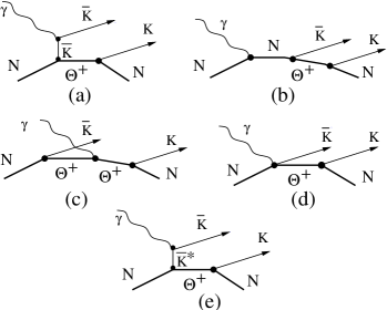
Figure 1: Tree-level diagrams for the reaction $\gamma N\to\Theta^{+}\bar{K}\to NK\bar{K}$.

Figure 2: Diagrams for the background process for the $\gamma N\to MN\to NK\bar{K}$ reaction, where $M$ denotes the mesons $\rho$, $\omega$, $\phi$, $\sigma$, $f_{2}$, and $a_{2}$.

We write $g_{\Theta NK^{*}}=\alpha g_{\Theta NK}$ in order to be able to pull out an overall factor of $g^{2}_{\Theta NK}$ from all contributions shown in Fig. 2. In view of the proportionality $g_{\Theta NK}^{2}\propto\Gamma_{\Theta}$, the dependence of the amplitudes on $\Gamma_{\Theta}$ then disappears if we consider the observables at the resonance position. The total amplitude depends on the relative-strength parameter $\alpha$ which will be fixed by experimental data. The dominance of the $K^{*}$ exchange channel Oh-2 ; CloseZhao allows us to reduce the number of relevant input parameters at a given coupling scheme to four: the sign and absolute value of $\alpha=g_{\Theta NK^{*}}/g_{\Theta NK}$ and the sign and absolute value of $\kappa^{*}$.

We will analyze two reactions, $\gamma p\to pK^{0}\bar{K}^{0}$ and $\gamma n\to nK^{+}K^{-}$, and we shall refer to them as the $\gamma p$ and the $\gamma n$ reactions, respectively.

In Sec. II, we describe our formalism. In Sec. III, we discuss the non-resonant background. The procedure to fix the parameters for the resonant amplitude is discussed in Sec. IV. The results of our numerical calculations for unpolarized and spin observables are presented in Sec. V. Our summary is given in Sec. VI. In Appendix A, we show an explicit form of the transition operators for the resonance amplitude. In Appendix B, we discuss the Pomeron exchange amplitude, and in Appendix C, we provide the parameters of the background amplitude.

II Formalism

II.1 Kinematics and cross sections

Figure 3: Schematic description of the $\Theta^{+}$ production in (a) the $\gamma N\to\bar{K}\Theta^{+}$ reaction in the center of mass system and in (b) the reaction $\gamma N\to NK\bar{K}$ in the $\Theta^{+}$ rest frame. The notations “P” and “D” correspond to the production and decay planes, respectively.

The scattering amplitude $T$ of the $\gamma N\rightarrow NK\bar{K}$ reaction is related to the $S$-matrix by

$$S_{fi}=\delta_{fi}-i(2\pi)^{4}\delta^{(4)}(k+p-q-\bar{q}-p^{\prime}){\cal T}_{fi}~{},$$ (1)

where $k$, $p$, $q$, $\bar{q}$, and $p^{\prime}$ denote the four-momenta of the incoming photon, the initial nucleon, the outgoing $K$ and $\bar{K}$ mesons, and the recoil nucleon, respectively. The standard Mandelstam variables for the virtual $\Theta^{+}$ photoproduction are defined by $t=(\bar{q}-k)^{2}$, $s\equiv W^{2}=(p+k)^{2}$. The $\bar{K}$ meson production angle $\theta$ in the center-of-mass system (cms) is given by $\cos\theta=\mathbf{k}\cdot\mathbf{\bar{q}}/|\mathbf{k}||\mathbf{\bar{q}}|$. The $\Theta^{+}$ decay distribution is described by the polar ($\Theta$) and azimuthal ($\Phi$) angles of the outgoing kaon, with solid-angle element $d\Omega_{Z}=d\cos\Theta\,d\Phi$. In the center-of-mass system, the quantization axis ($\bf z$) is chosen along the photon beam momentum, and the $\bf y$-axis is perpendicular to the production plane, i.e., $\bf y=k\times\bar{q}/|k\times\bar{q}|$. The $\Theta^{+}$ decay distribution is analyzed in the $\Theta^{+}$ rest frame, where the quantization axis $\bf Z$ is chosen along the incoming (target) nucleon and $\bf{Y}=\bf{y}$. For completeness, the production and decay planes with the corresponding coordinate systems are depicted in Fig. 3. We use the convention of Bjorken and Drell BD to define the $\gamma$ matrices; the Dirac spinors are normalized as $\bar{u}(p)\gamma_{\alpha}u(p)=2p_{\alpha}$. The invariant amplitude $T_{fi}$ is related to ${\cal T}_{fi}$ by

$${\cal T}_{fi}=\frac{T_{fi}}{\sqrt{(2\pi)^{15}\,2|\mathbf{k}|\,2E_{K}(\mathbf{q})\,2E_{\bar{K}}(\mathbf{\bar{q}}^{\prime})\,2E_{N}(\mathbf{p})\,2E_{N}(\mathbf{p}^{\prime})}}~{},$$ (2)

where $E_{i}(\mathbf{p})=\sqrt{M^{2}_{i}+\mathbf{p}^{2}}$, with $M_{i}$ denoting the mass of particle $i$. The differential cross section is related to the invariant amplitude by

$$\frac{d\sigma_{fi}}{d\Omega d\Omega_{Z}dM_{\Theta}}=\frac{p_{F}\sqrt{\lambda(s,M_{\Theta}^{2},M_{\bar{K}}^{2})}}{32(2\pi)^{5}W(W^{2}-M_{N}^{2})}\,\frac{1}{4}\sum_{m_{i},m_{f},\lambda_{\gamma}}|T_{fi}|^{2}~{},$$ (3)

where $\lambda(x,y,z)$ is the standard triangle kinematics function, $p_{F}=\sqrt{\lambda(M_{\Theta}^{2},M_{N}^{2},M_{K}^{2})}/2M_{\Theta}$ is the $\Theta^{+}$ decay momentum, $M_{\Theta}$ is the invariant mass of the outgoing nucleon and $K$-meson, $m_{i}$ and $m_{f}$ are the nucleon spin projections in the initial and the final states, respectively, and $\lambda_{\gamma}$ is the incoming photon helicity.

In the following, we consider the observables at the resonance position where the invariant mass of the outgoing nucleon and $K$ meson is equal to the $\Theta^{+}$ mass, $M_{\Theta}=M_{0}=1540$ MeV. In this case, the invariant amplitude of the resonant part is expressed through the $\Theta^{+}$ photoproduction (${A}$) and the $\Theta^{+}$ decay ($D$) amplitudes according to

$$T^{\pm}_{m_{f};m_{i},\lambda_{\gamma}}=\sum_{m_{\Theta}}\,{A}^{\pm}_{m_{\Theta};m_{i},\lambda_{\gamma}}\frac{1}{M_{\Theta}\Gamma_{\Theta}}D^{\pm}_{m_{\Theta};m_{f}}~{},$$ (4)

where plus (minus) corresponds to the positive (negative) $\Theta^{+}$ parity ($J^{P}=\frac{1}{2}^{\pm}$), $m_{\Theta}$ is the $\Theta^{+}$ spin projection. In the $\Theta^{+}$ rest frame, the decay amplitudes (p- and s-waves for the positive and negative $\Theta^{+}$ parity) read

$$\begin{split}\frac{1}{M_{\Theta}\Gamma_{\Theta}}D^{+}_{m;m_{f}}&=D^{0}\left(2m\,\delta_{m,m_{f}}\cos\Theta+\delta_{-m,m_{f}}\,\text{e}^{2im\Phi}\,\sin\Theta\right)~{},\\ \frac{1}{M_{\Theta}\Gamma_{\Theta}}D^{-}_{m;m_{f}}&=-D^{0}\,\delta_{m,m_{f}}~{},\qquad\qquad D^{0}=\sqrt{\frac{4\pi}{p_{F}\Gamma_{\Theta}}}~{},\end{split}$$ (5)

where $\Gamma_{\Theta}$ is the total width of the $\Theta^{+}$ decay. After integrating over the decay angles ($d\Omega_{Z}$) in Eq. (3), one obtains

$$\frac{d\sigma^{R}_{fi}}{d\Omega\,dM_{\Theta}}\Bigg{|}_{M_{\Theta}=M_{0}}=\frac{1}{\pi\Gamma_{\Theta}}\frac{d\sigma^{\Theta^{+}}_{fi}}{d\Omega}~{},$$ (6)

where

$$\frac{d\sigma^{\Theta^{+}}_{fi}}{d\Omega}=\frac{\sqrt{\lambda(s,M_{\Theta}^{2},M_{\bar{K}}^{2})}}{64\pi^{2}W^{2}(W^{2}-M_{N}^{2})}\,\frac{1}{4}\sum_{m_{i},m_{f},\lambda_{\gamma}}|{A}_{m_{f};m_{i},\lambda_{\gamma}}|^{2}$$ (7)

is the cross section of the $\Theta^{+}$ photoproduction in the $\gamma N\to\Theta^{+}\bar{K}$ reaction, with $m_{f}=m_{\Theta}$. By using the linear relation $g_{\Theta NK^{*}}=\alpha g_{\Theta NK}$, one finds that ${d\sigma^{R}}/{d\Omega\,dM_{\Theta}}$ does not depend on the $\Theta^{+}$ decay width at the resonance position, whereas ${d\sigma^{\Theta^{+}}}/{d\Omega}$ does.

II.2 Effective Lagrangians for the Resonant Amplitudes

As mentioned before, we describe the basic resonance process by considering the photoproduction of $\Theta^{+}$, with a subsequent decay of $\Theta^{+}$ into a nucleon and a kaon, as shown in Figs. 2a-d. We neglect, therefore, the contributions resulting from the photon interacting with the final decay vertex (see Ref. NT03 for the corresponding three additional graphs). In view of the chosen kinematics, where the invariant mass of the final $KN$ pair is at the resonance position, this is a good approximation since in the neglected graphs the $\Theta^{+}$ is far off-shell and the graphs of Figs. 2a-d dominate the resonance contribution. From a formal point of view, then, we lose gauge invariance of the process since this necessarily requires also the contributions arising from the electromagnetic interaction with the decay vertex. However, following Ref. hhgauge for the initial photoproduction process, we will construct an overall conserved current by an appropriate choice of the contact term of Fig. 2d. In view of the dominance of the resonance graphs we do take into account, numerically we expect very little difference between our present current-conserving results and those of a full gauge-invariant calculation.

The effective Lagrangians which define the amplitudes shown in Figs. 2a-d are discussed in Refs. Hosaka03 ; OKL031 ; NT03 ; LiuKo031 ; LiuKo032 ; LiuKo033 ; Zhao03 ; ZhaoKhal04 ; Oh-2 . Note, different papers employ different phase conventions. Therefore, for easy reference, we list here the explicit forms of the effective Lagrangians used in the present work. We have

$${\cal L}_{\gamma KK} = ie\,(K^{-}\partial^{\mu}K^{+}-K^{+}\partial^{\mu}K^{-})A_{\mu}~{},$$ (8a)

$${\cal L}_{\gamma\Theta\Theta} = -e\,\bar{\Theta}\left(\gamma_{\mu}-\frac{\kappa_{\Theta}}{2M_{\Theta}}\sigma_{\mu\nu}\partial^{\nu}\right)A^{\mu}\Theta~{},$$ (8b)

$${\cal L}_{\gamma NN} = -e\,\bar{N}\left(e_{N}\gamma_{\mu}-\frac{\kappa_{N}}{2M_{N}}\sigma_{\mu\nu}\partial^{\nu}\right)A^{\mu}N~{},$$ (8c)

$${\cal L}^{\pm[\text{pv}]}_{\Theta NK} = \mp\frac{g_{\Theta NK}}{M_{\Theta}\pm M_{N}}\bar{\Theta}\Gamma^{\pm}_{\mu}(\partial^{\mu}K)N+\text{h.c.}~{},$$ (8d)

$${\cal L}^{[\rm pv]}_{\gamma\Theta NK} = -i\frac{eg_{\Theta NK}}{M_{\Theta}\pm M_{N}}\bar{\Theta}\Gamma^{\pm}_{\mu}A^{\mu}KN+\text{h.c.}~{},$$ (8e)

$${\cal L}^{\pm[\text{ps}]}_{\Theta NK} = -i{g_{\Theta NK}}\bar{\Theta}\Gamma^{\pm}N+\text{h.c.}~{},$$ (8f)

where $A,\,\Theta$, $K$, and $N$ are the photon, $\Theta^{+}$, kaon, and the nucleon fields, respectively, $\Gamma^{\pm}_{\mu}\equiv\Gamma^{\pm}\gamma_{\mu}$ (with $\Gamma^{+}=\gamma_{5}$ and $\Gamma^{-}=1$ for positive and negative parity, respectively), $e_{p}=1$, $e_{n}=0$, and $\kappa_{N}$ is the nucleon anomalous magnetic moment ($\kappa_{p}=1.79$ and $\kappa_{n}=-1.91$). Equation (8e) describes the contact (Kroll-Ruderman) interaction in the pseudo-vector coupling scheme (see Fig. 2d), which is absent in case of the pseudo-scalar coupling [Eq. (8f)]. In addition, we consider the $K^{*}$ exchange process shown in Fig. 2e which is described by the two effective Lagrangians

$${\cal L}_{\gamma KK^{*}} = \frac{eg_{\gamma KK^{*}}}{M_{K^{*}}}\epsilon^{\alpha\beta\mu\nu}\partial_{\alpha}A_{\beta}\partial_{\mu}\bar{K}^{*}_{\nu}K+\text{h.c.}~{},$$ (9a)

$${\cal L}_{\Theta NK^{*}}^{\pm} = -g_{\Theta NK^{*}}\,\bar{\Theta}\,\Gamma^{\mp}\left(\gamma_{\mu}-\frac{\kappa^{*}}{M_{\Theta}+M_{N}}\sigma_{\mu\nu}\partial^{\nu}\right)\bar{K}^{*\mu}N+\text{h.c.}$$ (9b)

In calculating the invariant amplitudes we dress the vertices by form factors. In the present tree-level approach, with our chosen kinematics, only the lines connecting the electromagnetic vertex to the initial $\Theta^{+}KN$ vertex correspond to off-shell hadrons. We describe the product of both the electromagnetic and the hadronic form-factor contributions along these off-shell lines by the covariant phenomenological function

$$F(M,p^{2})=\frac{\Lambda^{4}}{\Lambda^{4}+(p^{2}-M^{2})^{2}}~{},$$ (10)

where $p$ is the corresponding off-shell four-momentum, $M$ is the mass, and $\Lambda$ is the cutoff parameter. We conserve the electromagnetic current of the entire amplitude by making the initial photoproduction process gauge invariant. To this end, we apply the gauge-invariance prescription by Haberzettl hhgauge , in the modification by Davidson and Workman DavWork (which renders the required additional contact terms free of kinematical singularities), to construct a contact term for the initial process $\gamma N\to\Theta^{+}\bar{K}$. For pseudovector coupling, the inclusion of form factors not only modifies the usual Kroll-Ruderman term, but also requires additional contact terms contributing to the amplitudes. We emphasize that contributions of the latter type are necessary even for pure pseudoscalar coupling.

The resonance amplitudes obtained for the $\gamma n$ and $\gamma p$ reactions read

$${A}^{\pm}_{fi}(\gamma n)=\bar{u}_{\Theta}(p_{\Theta})\left[{{{\cal M}^{s}}}^{\pm}_{\mu}+{{{\cal M}^{t}}}^{\pm}_{\mu}+{{{\cal M}^{u}}}^{\pm}_{\mu}+{{{\cal M}^{c}}}^{\pm}_{\mu}+{{{\cal M}^{t}}}^{\pm}_{\mu}(K^{*})\right]u_{p}(p)\varepsilon^{\mu},$$ (11a)

$${\cal A}^{\pm}_{fi}(\gamma p)=\bar{u}_{\Theta}(p_{\Theta})\left[{{{\cal M}^{s}}}^{\pm}_{\mu}+{{{\cal M}^{u}}}^{\pm}_{\mu}+{{{\cal M}^{c}}}^{\pm}_{\mu}+{{{\cal M}^{t}}}^{\pm}_{\mu}(K^{*})\right]u_{p}(p)\varepsilon^{\mu}~{}.$$ (11b)

The explicit forms of the transition operators ${\cal M}^{i}_{\mu}$ for the $\gamma n\to\Theta^{+}K^{-}\to nK^{-}K^{+}$ and $\gamma p\to\Theta^{+}\bar{K}^{0}\to pK^{0}\bar{K}^{0}$ reactions are shown in Appendix A. The choice of the strength parameters $g_{i}$ in the effective Lagrangians and the cutoff parameters $\Lambda=\Lambda_{B}$ will be discussed in Sec. IV.

III Non-resonant background

The non-resonant background for the reaction $\gamma n\to nK^{+}K^{-}$ has been discussed qualitatively by Nakayama and Tsushima NT03 . Together with the virtual vector-meson contribution $V\to K^{+}K^{-}$ ($V=\omega,\rho$, and $\phi$ mesons), they have included the excitation of the virtual $\Sigma$ hyperons. The coupling constants in the corresponding effective Lagrangians were fixed using the known decay widths and SU(3) symmetry, and the particles were taken as undressed but with physical masses. The present analysis with dressing form factors shows that at $E_{\gamma}\approx 2$ GeV, the main contribution comes from the virtual vector-meson photoproduction. For completeness, we also explore the contribution from the scalar ($\sigma$) and tensor ($a_{2},f_{2}$) mesons. As we shall show in Sec. III.E, the latter is found to be negligibly small in the $E_{\gamma}\approx 2$ GeV region.

III.1 Vector meson contributions: $\rho,\omega,\phi$

Figure 4: The phase-space diagram for the $\Theta^{+}$ photoproduction at $E_{\gamma}=2$ GeV: the invariant mass $M_{K\bar{K}}$ versus $\cos\Theta$ at a fixed $\bar{K}$ production angle ($\theta=55^{\circ}$). The cutoff area of the phase phase is placed between the two solid lines.

Naively, one can expect the dominance of the intermediate $\rho$-meson channel in the background contribution because the cross section for the real $\rho$-meson photoproduction is about an order of magnitude larger than that for the $\omega$ meson, and it is about two orders of magnitude larger than that for the $\phi$-meson photoproduction. However, at $E_{\gamma}\approx 2$ GeV, the $K\bar{K}$ invariant mass is distributed in the region $1\,\text{GeV}\lesssim M_{K\bar{K}}\lesssim 1.2$ GeV which straddles the $\phi$ mass. Fig. 4 shows an example of the phase-space diagram of the $K\bar{K}$ invariant mass versus the cosine of the $K$ decay angle at a fixed $\bar{K}$production angle of $\theta(\text{cm})=55^{\circ}$. One can see that the narrow mass distribution of the $\phi$ is within the sampled kinematic region which therefore makes the $\phi$-meson contribution significant.

In this study we consider the contribution from $\rho,\,\omega$, and $\phi$ mesons. The low-energy $\rho$- and $\omega$-meson photoproductions are described within an effective meson-exchange model TLTS99 ; TitovLee02 ; FS96 . Thus, the $\rho$-meson photoproduction is dominated by the $t$-channel scalar ($\sigma$) and pseudoscalar ($\pi$) meson exchanges. The $\omega$-meson photoproduction is mostly defined by the $\pi$ exchange. In Ref. Oh04 the $\sigma$ exchange in the $\rho$ photoproduction is reexamined on the basis of un-correlated two-pion and tensor $f_{2}$-meson exchanges. The main problem of this approach is the requirement of a large coupling constant for the $f_{2}\rho\gamma$ interaction. This results in a branching ratio of $f_{2}\to\rho\gamma$ decay which seems to be unreasonably large. Another ambiguity is related to the unknown $f_{2}NN$ coupling and the form factors for the off-shell $f_{2}$ meson. Since the quality of the description of the experimental data using either the $\sigma$ exchange or the $f_{2}$ exchange is comparable to each other Oh04 , and to avoid introducing too many unknown parameters, we employ the $\sigma$-exchange model in this work; this is quite reasonable for the present purposes. When the photon energy increases, we have to add the Pomeron exchange as well. But at $E_{\gamma}\approx 2$ GeV, it is important only for the $\rho$ channel where the Pomeron exchange gives about 30% of its contribution. In the $\omega$ channel, the Pomeron contribution is suppressed by the factor $(\gamma_{\rho}/\gamma_{\omega})^{2}\approx 6.33/72.71\approx 1/11.5$, where $\gamma_{\rho}$ and $\gamma_{\omega}$ are the $\rho$ and $\omega$ decay couplings, respectively. Therefore, in the $\omega$ photoproduction, we limit ourselves to the $\pi$ exchange process only. The effective Lagrangians responsible for the meson-exchange channels read

$${\cal L}_{\pi NN} = \frac{g_{\pi NN}}{M_{N}}\bar{N}\gamma_{5}\gamma_{\mu}\partial^{\mu}\pi N~{},$$ (12a)

$${\cal L}_{\sigma NN} = g_{\sigma NN}\bar{N}N\sigma~{},$$ (12b)

$${\cal L}_{\rho\sigma\gamma} = \frac{eg_{\rho\sigma\gamma}}{2M_{\rho}}(\partial^{\nu}\rho^{\mu}-\partial^{\mu}\rho^{\nu})(\partial_{\nu}A_{\mu}-\partial_{\mu}A_{\nu})\sigma~{},$$ (12c)

$${\cal L}_{V\pi\gamma} = \frac{eg_{V\pi\gamma}}{M_{V}}\epsilon^{\alpha\beta\mu\nu}\partial_{\alpha}A_{\beta}\partial_{\mu}V_{\nu}\pi~{},$$ (12d)

$${\cal L}_{VKK} = ig_{VKK}(\bar{K}\partial^{\mu}K-K\partial^{\mu}\bar{K})V_{\mu}~{},$$ (12e)

where $V$ stands for the vector meson. The amplitudes for the $\gamma N\to NV\to NK\bar{K}$ reaction may be expressed as

$$T_{fi}=\sum\limits_{\lambda_{V}}A^{V}_{m_{f}\lambda_{V};m_{i}\lambda_{\gamma}}\frac{1}{M^{2}_{V}-M_{K\bar{K}}^{2}+i\Gamma_{V}M_{V}}D^{V}_{\lambda_{V}}\,F_{V}(M^{2}_{K\bar{K}})~{},$$ (13)

where $A^{V}$ and $D^{V}$ are the vector meson photoproduction ($\gamma N\to VN$) and decay ($V\to K\bar{K}$) amplitudes, respectively, $M_{K\bar{K}}$ is the $K\bar{K}$ invariant mass, $\Gamma_{V}$ is the total decay width of the vector meson, $\lambda_{\gamma}$ and $\lambda_{V}$ are the helicities of the photon and vector meson, respectively, and $F_{V}$ is the form factor of the virtual vector meson.

The photoproduction amplitudes may be expressed in a standard form

$$A^{V}_{m_{f}\lambda_{V};m_{i}\lambda_{\gamma}}=\bar{u}_{f}{\cal M}_{\mu\nu}u_{i}\,\varepsilon^{\mu}_{\lambda_{\gamma}}{\varepsilon^{*}}^{\nu}_{\lambda_{V}}~{}.$$ (14)

In the case of the scalar (S: $\sigma$) and pseudoscalar (PS: $\pi$) meson exchange, the transition operators ${\cal M}_{\mu\nu}$ read

$${\cal M}_{\mu\nu}^{\text{S}} = \frac{eg_{\rho\sigma\gamma}g_{\sigma NN}}{M_{\rho}}\frac{g_{\mu\nu}(k\cdot Q_{V})-{Q_{V}}_{\mu}k_{\nu}}{\bar{t}-M^{2}_{\sigma}}F_{\sigma}(\bar{t})~{},$$ (15)

$${\cal M}_{\mu\nu}^{\text{PS}} = i\frac{eg_{\rho\pi\gamma}g_{\pi NN}}{M_{\rho}}\gamma_{5}\frac{\varepsilon^{\mu\nu\alpha\beta}k_{\alpha}{Q_{V}}_{\beta}}{\bar{t}-M^{2}_{\pi}}F_{\pi}(\bar{t})~{},$$ (16)

respectively, where $Q_{V}=q+\bar{q}$, and $F_{M}$ is the product of the two form factors of the virtual exchanged mesons in the $MNN$ and $\gamma VM$ vertices. The explicit forms of $F_{M}(\bar{t})$ are given in Appendix C. Note that the four-momentum transfers to the $K\bar{K}$ pair, $\bar{t}$ is different from $t$ in $\Theta^{+}$ photoproduction.

The decay amplitude,

$$D^{V}_{\lambda_{V}}=g_{VKK}(q-\bar{q})_{\mu}\varepsilon^{\mu}_{\lambda_{V}}~{},$$ (17)

has a simple form in the $V$ rest frame, with the quantization axis $\mathbf{z}$ parallel to the beam momentum (Gottfried-Jackson system), i.e.,

$$D^{V}_{\lambda_{V}}=2k_{f}g_{VKK}\sqrt{\frac{4\pi}{3}}Y_{1\lambda_{V}}(\widehat{\mathbf{q}})~{},\qquad k_{f}=\frac{M_{K\bar{K}}}{2}\sqrt{1-4\frac{M_{K}^{2}}{M^{2}_{K\bar{K}}}}~{},$$ (18)

where $\widehat{\mathbf{q}}$ is the solid angle of the direction of flight of the $K$ meson in the $K\bar{K}$ rest frame, i.e., $\widehat{\mathbf{q}}\equiv\Omega_{K}$. The $\phi$-meson photoproduction is defined by the Pomeron and pseudoscalar ($\pi,\eta$) meson exchanges, as described in Ref. Titov03 . For an easy reference, we provide the transition operator ${\cal M}^{P}_{\mu\nu}$ for the Pomeron exchange amplitude and the parameters which define the $\phi$-, $\rho$-, and $\omega$-meson photoproduction in Appendices B and C, respectively.

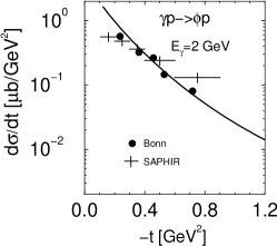
Figure 5: Cross sections for the $\rho$-, $\omega$-, and $\phi$-meson photoproduction. The experimental points are taken from Refs. SAPHIR ; BONN ; SAPHIR2 .

Figures 5a-c show the cross sections of the vector-meson photoproduction in the reactions $\gamma p\to Vp$ ($V=\rho,\omega,\phi$) at $E_{\gamma}\approx 2$ GeV together with the available data. One can see a quite reasonable agreement between the experimental data and the calculation. This encourages us to use the same model for the description of the non-resonant background in the $\Theta^{+}$ photoproduction.

III.2 Scalar meson contribution: $\sigma$

The $\gamma\rho\sigma$ interaction responsible for the $\rho$-meson contribution naturally leads to the virtual $\sigma$-meson photoproduction and its subsequent decay into the $K\bar{K}$ pair as shown in Fig. 2d. The corresponding effective Lagrangians for this transition read

$${\cal L}_{\sigma KK} =M_{\sigma}g_{\sigma KK}\sigma K\bar{K}~{},$$ (19a)

$${\cal L}_{\rho NN} =-g_{\rho NN}\left(\bar{N}\gamma_{\mu}\rho^{\mu}N-\frac{\kappa_{\rho}}{2M_{N}}\bar{N}\sigma_{\mu\nu}\partial^{\nu}\rho^{\mu}N\right)~{}.$$ (19b)

The $\sigma K\bar{K}$ coupling may be estimated from SU(3) symmetry as $g_{\sigma KK}=-g_{\sigma\pi\pi}/2$.

The amplitude for the $\gamma N\to\sigma N\to NK\bar{K}$ process has the form

$$A_{m_{f};m_{i}\lambda_{\gamma}}=\bar{u}_{f}{\cal M}^{\rho}_{\mu}u_{i}\varepsilon^{\mu}_{\lambda_{\gamma}}~{},$$ (20)

where

$${\cal M}_{\mu}^{\rho}=\frac{eg_{\rho\sigma\gamma}g_{\rho NN}}{M_{\rho}(\bar{t}-M_{\rho}^{2})}\left[{(1+\kappa_{\rho})\hat{R}_{\mu}-{\kappa_{\rho}}\frac{R^{\prime}_{\mu}}{M_{N}}}\right]F_{\rho}(\bar{t})~{},$$ (21)

with

$$\hat{R}_{\mu} =(k\cdot Q)\gamma_{\mu}-k\!\!\!/Q_{\mu}~{},$$ (22a)

$$R^{\prime}_{\mu} =(k\cdot Q)p^{\prime}_{\mu}-(k\cdot p^{\prime})Q_{\mu}~{},$$ (22b)

$$Q =p^{\prime}-p~{}.$$ (22c)

The $\sigma\to K\bar{K}$ decay amplitude is a constant

$$D_{\sigma}=-M_{\sigma}g_{\sigma KK}\sqrt{4\pi}Y_{00}(\widehat{\mathbf{q}})~{}.$$ (23)

For the vector and tensor coupling constants and the cutoff parameter in $F_{\rho}$, we take the corresponding values from the Bonn model BonnMod (see Appendix C).

III.3 Tensor meson contributions: $a_{2}$, $f_{2}$

The tensor $a_{2}(1320)$ and $f_{2}(1270)$ mesons have finite branching ratios into the $K\bar{K}$ decay channel and, therefore, one can expect their non-negligible contributions to the non-resonant background in the $\Theta^{+}$ photoproduction Dzierba04 . The corresponding branching ratios are $(4.9\pm 0.8)\times 10^{-2}$ and $(4.6\pm 0.5)\times 10^{-2}$ for the $a_{2}(1320)$ and $f_{2}(1270)$ mesons, respectively PDG .

Similarly to the scalar meson, the tensor mesons ($a_{2}$ and $f_{2}$) appear in the “non-resonant” background in two ways. Firstly, $a_{2}$ and $f_{2}$ give a contribution to the photoproduction of the $\omega$ and $\rho$ mesons , respectively. Secondly, they can be produced directly by the incoming photon with subsequent exchange by $\omega$ and $\rho$ mesons, as it is depicted in Fig. 2e,f. The first case results only in some renormalization of the coupling constants in the $\omega$ and $\rho$ photoproduction amplitudes, and it does not modify the shape of the $K\bar{K}$ invariant mass distribution. But since the coupling constants in the $\rho$ and $\omega$ photoproduction processes are fixed by the corresponding experimental data anyway, we may assume that such a renormalization effect is taken into account in those effective strength parameters. The second contribution may change the $K\bar{K}$ invariant distribution qualitatively when $M_{K\bar{K}}\approx M_{f_{2}(a_{2})}$. This is realized at higher energies with $E_{\gamma}\geq 2.3$ GeV. At $E_{\gamma}\approx 2$ GeV, their contribution is not very strong; nevertheless, for completeness, we include these processes in our consideration. We assume that production of the $a_{2}$ and $f_{2}$ mesons is generated by the $a_{2}\gamma\omega$ and $f_{2}\gamma\rho$ interactions, respectively.

The interaction of the tensor and the two vector fields is described by the gauge-invariant interaction

$$\begin{split}{\cal L}_{t_{2}V_{1}V_{2}}&=\frac{g_{t_{2}V_{1}V_{2}}}{M_{t_{2}}}(L^{\alpha\beta}+L^{\beta\alpha})\xi_{\alpha\beta}~{},\\ L^{\alpha\beta}&=(\partial^{\alpha}V_{1}^{\mu}-\partial^{\mu}V_{1}^{\alpha})(\partial^{\beta}{V_{2}}_{\mu}-\partial_{\mu}V_{2}^{\beta})~{},\end{split}$$ (24)

where $V_{1,2}$ and $\xi$ are the vector and tensor meson fields, respectively, and $t_{2}=a_{2},f_{2}$.

The $t_{2}K\bar{K}$ interaction is described by the effective Lagrangian

$${\cal L}_{t_{2}KK}=\frac{g_{t_{2}KK}}{M_{t_{2}}}\left(\partial^{\beta}\bar{K}\partial^{\alpha}K+\partial^{\beta}K\partial^{\alpha}\bar{K}\right)\xi_{\alpha\beta}~{}.$$ (25)

The coupling constant $g_{t_{2}KK}$ is related to the decay width $\Gamma_{t_{2}\to K\bar{K}}$ width that subsumes transitions into both $K^{0}\bar{K}^{0}$ and $K^{+}K^{-}$ channels according to

$${g^{2}_{t_{2}KK}}=\frac{15\pi\Gamma_{t_{2}\to K\bar{K}}M_{t_{2}}^{4}}{2p_{t_{2}}^{5}}~{},$$ (26)

where $p_{t_{2}}=M_{t_{2}}\sqrt{1/4-M_{K}^{2}/M^{2}_{t_{2}}}$ is the $t_{2}$ decay momentum. Here we assume that $\Gamma_{t_{2}\to K^{+}K^{-}}\approx\Gamma_{t_{2}\to K^{0}\bar{K}^{0}}\approx 0.5\Gamma_{t_{2}\to K\bar{K}}$. Using the known widths $\Gamma_{a_{2}\to K\bar{K}}$ and $\Gamma_{f_{2}\to K\bar{K}}$ from PDG we get

$${g_{a_{2}KK}}=4.9~{},\qquad{g_{f_{2}KK}}=7.4~{}.$$ (27)

The amplitude of the $\gamma N\to Nt_{2}\to NK\bar{K}$ transition is expressed as

$$T_{fi}=\sum\limits_{\lambda_{\gamma}\sigma}A^{t_{2}}_{m_{f}\sigma;m_{i}\lambda_{\gamma}}\frac{1}{M^{2}_{t_{2}}-M_{K\bar{K}}^{2}+i\Gamma_{t_{2}}M_{t_{2}}}D^{t_{2}}_{\sigma}\,F_{t_{2}}(M^{2}_{K\bar{K}})~{},$$ (28)

where $A^{t_{2}}$ is the tensor meson photoproduction ($\gamma N\to t_{2}N$) amplitude, $\Gamma_{t_{2}}$ is the total decay width of the tensor meson, $\sigma$ is the spin projection of the tensor meson, and $F_{t_{2}}$ is the form factor of the virtual tensor meson. The $t_{2}\to K\bar{K}$ decay amplitude reads

$$D^{t_{2}}_{\sigma}=-\frac{2g_{t_{2}KK}k_{f}^{2}}{M_{t_{2}}}\sqrt{\frac{8\pi}{15}}Y_{2\sigma}(\widehat{\mathbf{q}})~{},$$ (29)

The $a_{2}$-meson photoproduction amplitude is given by

$$A^{a_{2}}_{m_{f}\sigma;m_{i}\lambda_{\gamma}}=\frac{g_{a_{2}\gamma\omega}g_{\omega NN}}{M_{a_{2}}}\bar{u}_{f}H^{a_{2}}_{\alpha\beta\mu}\,u_{i}\,\varepsilon^{*\alpha\beta}\,\varepsilon^{\mu}_{\lambda_{\gamma}}\,F_{\omega}(\bar{t})~{},$$ (30)

where $\varepsilon^{\alpha\beta}$ is the Rarita-Schwinger spinor of the tensor meson

$$\varepsilon_{\alpha\beta}(\sigma)=\sum\limits_{l_{1}l_{2}}\langle 1l_{1}\,1l_{2}|2\sigma\rangle\,\varepsilon_{\alpha}(l_{1})\varepsilon_{\beta}(l_{2})~{},$$ (31)

and

$$H^{a_{2}}_{\alpha\beta\mu}=(Q_{\alpha}\gamma^{\nu}-Q^{\nu}\gamma_{\alpha})(k_{\beta}g_{\mu\nu}-k_{\nu}g_{\mu\beta})+(Q_{\beta}\gamma^{\nu}-Q^{\nu}\gamma_{\beta})(k_{\alpha}g_{\mu\nu}-k_{\nu}g_{\mu\alpha})~{}.$$ (32)

Similarly, the amplitude of the $f_{2}$-meson photoproduction reads

$$A^{f_{2}}_{m_{f}\sigma;m_{i}\lambda_{\gamma}}=\frac{g_{f_{2}\gamma\rho}g_{\rho NN}}{M_{f_{2}}}\bar{u}_{f}H^{f_{2}}_{\alpha\beta\mu}\,u_{i}\,\varepsilon^{*\alpha\beta}\,\varepsilon^{\mu}_{\lambda_{\gamma}}\,F_{\rho}(\bar{t})~{},$$ (33)

with

$$\begin{split}H^{f_{2}}_{\alpha\beta\mu}&=(Q_{\alpha}G^{\nu}-Q^{\nu}G_{\alpha})(k_{\beta}g_{\mu\nu}-k_{\nu}g_{\mu\beta})+(Q_{\beta}G^{\nu}-Q^{\nu}G_{\beta})(k_{\alpha}g_{\mu\nu}-k_{\nu}g_{\mu\alpha})~{},\\ G_{\mu}&=(1+\kappa_{\rho})\gamma_{\mu}-\frac{\kappa_{\rho}}{M_{N}}p^{\prime}_{\mu}~{}.\end{split}$$ (34)

In the absence of experimental information necessary to extract the coupling constants $g_{a_{2}\gamma\omega}$ and $g_{f_{2}\gamma\rho}$, we assume that

$$eg_{a_{2}\omega\gamma}=0.29~{},\qquad eg_{f_{2}\rho\gamma}=0.14~{}.$$ (35)

These are rough estimates obtained by making use of the available data for the decay widths for $a_{2}\to\omega\pi^{+}\pi^{-}$, $a_{2}\to\gamma\gamma$, and $f_{2}\to\gamma\gamma$ in conjunction with the vector dominance model, in addition to the Gell-Mann–Sharp–Wagner contact term GSW .

III.4 $K\bar{K}$ invariant mass distribution

If there is no limitation on the phase space of the outgoing kaons, then the integration over the decay angle of the $K$ meson eliminates the interference terms among the scalar, vector, and tensor meson exchange contributions, and the $K\bar{K}$ invariant mass distribution may be expressed in a compact form as

$$\frac{64\pi^{3}(s-M_{N}^{2})^{2}}{k_{f}}\,\frac{d\sigma}{d\bar{t}\,dM_{K\bar{K}}} =M_{\sigma}^{2}g^{2}_{\sigma KK}\frac{|A_{\sigma}|^{2}}{(M_{K\bar{K}}^{2}-M_{\sigma}^{2})^{2}+M_{\sigma}^{2}\Gamma_{\sigma}^{2}}$$

$$\quad\mbox{}+\frac{4k_{f}^{2}}{3}\left|\sum\limits_{V}\frac{g_{VKK}A^{V}_{fi}}{M_{K\bar{K}}^{2}-M_{V}^{2}+iM_{V}\Gamma_{V}}\right|^{2}$$

$$\quad\mbox{}+\frac{8k_{f}^{2}}{5}\left|\sum\limits_{t_{2}}\frac{k_{f}}{M_{t_{2}}}\frac{g_{t_{2}KK}A^{t_{2}}_{fi}}{M_{K\bar{K}}^{2}-M_{t_{2}}^{2}+iM_{t_{2}}\Gamma_{t_{2}}}\right|^{2}~{},$$ (36)

where the average over the spins/helicity in the initial state and the summation over spin variable in the final states are implied. One can see that, near threshold, the tensor meson contribution is suppressed by the factor $k_{f}^{2}/M_{t_{2}}^{2}\ll 1$ compared to the vector meson contribution.

Figure 6: (a) Dependence of the shape of the invariant mass distribution on the cutoff parameter $\Lambda_{0}$ in the $\gamma n\to K^{+}K^{-}$ reaction. (b) $K\bar{K}$ invariant-mass distribution in $\gamma n\to K^{+}K^{-}$ taken from Ref. Nakano03 ; arrows indicate the $\phi$-meson cut window.

  

Figure 7: $K\bar{K}$ invariant-mass distribution in (a) $\gamma n\to K^{+}K^{-}$ and in (b) $\gamma p\to pK^{0}\bar{K}^{0}$. The arrows indicate the $\phi$-meson cut window.

The $K\bar{K}$ invariant mass distribution at a forward angle of $K\bar{K}$ photoproduction [$\theta_{K\bar{K}}\,(\rm cm)=10^{\circ}$] is shown in Figs. 7 and 7. The photon energy was taken from the threshold to 2.35 GeV, in accordance with the measurement of Ref. Nakano03 . The distribution has one unknown parameter compared to the real vector meson photoproduction. It is the cutoff parameter $\Lambda_{0}$ in the form factor $F_{(V,\sigma,a_{2},f_{2})}=F(M_{(V,\sigma,a_{2},f_{2})},M^{2}_{K\bar{K}})$, where $F(M,x^{2})$ is defined in Eq. (10). The dependence of the $K\bar{K}$ invariant mass on this parameter is shown in Fig. 7a. A comparison with the measured distribution Nakano03 shown in Fig. 7b favors $\Lambda_{0}\approx 0.9$ GeV. We use this value in our further analysis. Figures 7a,b show the structure of these distributions. One can see a strong $\phi$-meson photoproduction peak at $M_{K\bar{K}}\approx M_{\phi}$ and a long tail dominated by the $\rho$-meson channel. The contribution from the other mesons is much smaller. The contribution from the $a_{2}$ and $f_{2}$ mesons becomes comparable to that from the vector mesons near the threshold, $M_{K\bar{K}}\approx 1.3$ GeV (at $E_{\gamma}=2.2$ GeV). In this region of the $K\bar{K}$ invariant masses, the cross section is rather small compared to that around $M_{K\bar{K}}\approx M_{\phi}$, which gives the main contribution to the background of the $\Theta^{+}$ photoproduction at $E_{\gamma}\approx 2$ GeV.

Finally, we note that the cross section for $\gamma n\to nK^{+}K^{-}$ exceeds that for $\gamma p\to pK^{0}\bar{K}^{0}$ by approximately a factor of two. This is due to the distinct $\phi-\rho$ interference effect in these two reactions caused by the different signs in the $\rho K^{+}K^{-}$ and $\rho K^{0}\bar{K}^{0}$ coupling constants. In the case of the $\phi$-meson, the signs of the $\phi K^{+}K^{-}$ and $\phi K^{0}\bar{K}^{0}$ coupling constants are the same.

III.5 Non-resonant background in $\Theta^{+}$ photoproduction

Let us now examine the background contribution to the angular distribution of the $K\bar{K}$ pair in the final state. The $K\bar{K}$ invariant mass is taken at the $\Theta^{+}$ resonance position at $M_{\Theta}=M_{0}=1.54$ GeV. The corresponding differential cross section, $d\sigma/d\Omega\,dM_{\Theta}$, where $\Omega$ is the solid angle of the $K\bar{K}$ pair, is calculated using the general expression for the differential cross section given by Eq. (3). Here, all the background channels contribute coherently and the integration over the $\Theta^{+}$ decay angle $\Omega_{Z}$ is performed numerically.

Figure 8: Contribution of the background processes to the differential cross section of the $\Theta^{+}$ photoproduction for the (a,b) $\gamma n$ and (c) $\gamma p$ reactions without (a) and with (b,c) the cut in the $K\bar{K}$ invariant-mass distribution, respectively.

Our result for the $\gamma n\to nK^{+}K^{-}$ reaction is shown in Fig. 8a. One can see a rather strong contribution from the $\phi$ photoproduction. We will eliminate the phase space with the $K\bar{K}$ invariant mass from 1.00 to 1.04 GeV following Ref. Nakano03 in order to reduce its contribution. The corresponding phase space, shown schematically in Fig. 4, is about 15% of the total phase space but it gives about 100% of the $\phi$-channel contribution to the background. The differential cross section, with an $M_{K\bar{K}}$ cut for the $\gamma n$ and $\gamma p$ reactions, are shown in Figs. 8b and 8c, respectively. Now the $\phi$ and $\rho$ contributions are comparable to each other. Another interesting aspect is the enhancement of the $\sigma$ contribution compared to the corresponding contribution in the case of the $K\bar{K}$ invariant-mass distributions shown in Fig. 7a,b. This enhancement is explained by the term ${\kappa_{\rho}}(R^{\prime}\cdot\varepsilon_{\gamma})/M_{N}$ in Eq. (20) caused by the $\rho NN$ tensor coupling. The contribution from this term increases strongly with increasing $|\mathbf{p}^{\prime}|\sin\theta_{K}$. When the momentum transfer to the $K\bar{K}$ pair is small (see Fig. 7a,b), this contribution is rather small, whereas in the kinematic condition of Fig. 8 it is large.

As can be seen from Fig. 8 and from the discussion in connection to Fig. 7a,b in Sec. III.D, the contributions from the tensor mesons, $a_{2}$ and $f_{2}$, at $E_{\gamma}\approx 2$ GeV are found to be very small (even for large coupling constants Oh04 and different choices of their signs). Therefore, hereafter, the tensor mesons will be omitted in our calculations.

IV Fixing the parameters of the resonant amplitude

(1) The magnitude of the coupling constant, $g_{\gamma KK^{*}}$, is extracted from the width of the $K^{*}\to\gamma K$ decay PDG . Its sign is fixed by SU(3) symmetry. We have $eg_{\gamma K^{0}K^{*0}}=-0.35$ and $eg_{\gamma K^{\pm}K^{*\pm}}=0.23$.

(2) The contribution of the $s$-channel (Fig. 2b) is small which leads to a rather weak dependence of the total amplitude on the tensor coupling $\kappa_{\Theta}$ in the $\gamma\Theta\Theta$ interaction within a “reasonable” range of $0\lesssim|\kappa_{\Theta}|\lesssim 0.5$ MagMom . Therefore, we choose $\kappa_{\Theta}=0$ for both parities.

(3) The coupling constant $g_{\Theta NK}$ for the positive and negative $\Theta^{+}$ parity is found from the $\Theta^{+}$ decay width,

$$\Gamma_{\Theta}=\frac{[g^{\pm}_{\Theta NK}]^{2}p_{F}}{2\pi M_{\Theta}}(\sqrt{M_{N}^{2}+p_{F}^{2}}\mp M_{N})~{}.$$ (37)

There are several indications that the $\Theta^{+}$ decay width is most likely to be of the order of one MeV SmallWidth and that the observed width $\Gamma_{\text{exp}}$ in the $\Theta$ photoproduction is rather to be regarded as the experimental resolution ($\Delta$). By construction (see Introduction), the differential cross section for the $\Theta^{+}$ photoproduction defined by Eq. (3) at the resonance position does not depend on the $\Theta$ decay width. Instead, it depends on the ratio of the coupling constants $g_{\Theta NK^{*}}$ and $g_{\Theta NK}$ (as well as, in general, also on other parameters). In principle, this ratio may be extracted from the experimental data by comparing the resonant and the background contributions because the cross section due to the background is known in the present case. However, a proper comparison requires to account for the “experimental resolution” in our calculation. The smearing of the $\Theta^{+}$ invariant mass distribution results in a suppression of the resonant cross section at the resonance position by a factor of

$$d^{2}\approx\frac{\Gamma_{\Theta}}{\Delta}\approx\frac{1}{10}~{},$$ (38)

where we use an averaged value of $\Delta\approx 20$ MeV and $\Gamma_{\Theta}\approx 2$ MeV. We include the effect of this smearing by multiplying all the resonance amplitudes by this factor $d$. In our calculation we will use the ratio of the resonance plus background to background processes from the experiment to fix the model parameters. This ratio is different in different experiments and varies from 2 CLAS1 to 7 SAPHIR03 . We will use a value of 3.4 which corresponds to that found in the LEPS experiment.

(4) The next important point is to fix the cutoff parameters. In our model, we have two different cutoff parameters. One ($\Lambda_{K^{*}}$) is in the $t$-channel $K^{*}$ exchange amplitude. Another one ($\Lambda_{B}$) defines the Born terms of the $s$-, $u$-, and $t$-channels and the current-conserving contact terms $c$. Generally speaking, $\Lambda_{K^{*}}$ together with $g_{\Theta NK*}$ (or the ratio $\alpha=g_{\Theta NK^{*}}/g_{\Theta NK}$) defines the strength of the $K^{*}$ exchange amplitude. Increasing $\Lambda_{K^{*}}$ leads to a decreasing $\alpha$. If we assume for the moment that the Born terms are negligible compared to the $K^{*}$ exchange, then taking as a guide the quark model prediction for $\alpha$ for the positive $\Theta^{+}$ parity QMKK* ,

$$\alpha\approx\sqrt{3}~{},$$ (39)

we can fix $\Lambda_{K^{*}}$ using the calculated background cross section and measured ratio of the resonance contribution to the background [signal-to-noise ($S/N$)]. The $\gamma p\to pK^{0}\bar{K}^{0}$ reaction is close to this ideal case, where the $K^{*}$-exchange contribution is much larger than the Born terms. But in the case of the $\gamma n\to nK^{+}\bar{K}^{-}$ reaction, the situation is more complicated. The $t$-channels and the contact terms are strong and comparable to the $K^{*}$ exchange. These situations for the $\gamma p$ and $\gamma n$ reactions may be understood from Fig. 9. We show here the differential cross sections for the $\gamma N\to NK\bar{K}$ reactions as a function of $\bar{K}$-production angle in the center-of-mass system at the resonance position and for positive and negative $\Theta^{+}$ parities. We display the individual contributions from the Born terms, the $K^{*}$ exchange channel and the background processes for both the pseudoscalar and pseudovector couplings with $\Lambda_{B}=1$ GeV. The parameters for the $K^{*}$ exchange amplitude read $\Lambda_{K}^{*}=1.5$, $\alpha=1$ and $\kappa^{*}=0$. One can see that for the $\gamma p$ reactions the $K^{*}$-exchange channel is dominant, whereas for the $\gamma n$ reactions all the individual contributions become comparable to each other and the problem of fixing the cut off parameter $\Lambda_{B}$ must be solved consistently. Note that the inclusion of the $\Sigma$ and $\Lambda$ photoproduction LambdaSigma processes results in a larger ambiguity in the choice of $\Lambda_{B}$ which varies from 0.5 to 2 (GeV) depending on the coupling scheme, method of conserving the electromagnetic current, etc.

Figure 9: Contributions of the Born $s$, $t$, $u$ and the contact $c$ terms in the (a,b) $\gamma p$ and (c,d) $\gamma n$ reactions, together with the $t$-channel $K^{*}$ exchange and the background processes. The respective cases for positive and negative $\pi_{\Theta}$ are depicted in (a,c) and (b,d).

To choose $\Lambda_{B}$, we use the following strategy. We assume that the ratio $\alpha$, as well as the cutoff $\Lambda_{K^{*}}$, must be the same in the $\gamma p$ and $\gamma n$ reaction. Then, fixing $\alpha$ and $\Lambda_{K^{*}}$ from the $\gamma p$ reaction and using the signal-to-noise ratio $S/N$, we determine $\Lambda_{B}$ unambiguously for the $\gamma n$ reaction and its value will depend on the type of the coupling (PV or PS), the value and the sign of tensor coupling ($\kappa^{*}$), and sign of $\alpha$.

Figure 10: The scale parameter $\alpha$ as a function of the cutoff parameters $\Lambda_{K^{*}}$ and $\Lambda_{B}$.

Figure 11: The cross section of the resonance $\Theta^{+}$ photoproduction and the background processes as a function of the $\bar{K}$-production angle for the (a,b) $\gamma p$ and (c,d) $\gamma n$ reactions and for the (a,c) positive and (b,d) negative parities of $\Theta^{+}$.

Figure 10 shows the dependence of $\alpha$ on $\Lambda_{B}$ at fixed $\Lambda_{K^{*}}$ and $\kappa^{*}=0$. For the $\gamma p$ reaction, this dependence is rather weak but for $\gamma n$, it is strong. For further analysis of the $\gamma p$ reaction, we chose an averaged value of $\Lambda_{B}=1$ GeV. We will analyze observables at three values of the tensor coupling $\kappa^{*}=0,\pm 0.5$. The corresponding values of $\alpha$ depending on $\kappa^{*}$ and the $\Theta^{+}$ parity are shown in Table 1. All the calculations are done at the $\bar{K}$ production angle of $\theta=55^{\circ}$, where the resonance processes are largest. Also, at this condition, the background contribution is dominated by the known $\phi$ and $\rho$ channels and therefore it is better established. Figures 11a-d show the result for the differential cross section for the $\gamma N\to NK\bar{K}$ reactions, calculated by considering a coherent sum of all the resonance processes with the scaled $K^{*}$ exchange amplitude by a factor of $\alpha$ and appropriate $\Lambda_{B}$. One can see that in the vicinity of $\theta\approx 55^{\circ}$, the unpolarized cross sections for the different coupling schemes and different parities are close to each other for both the $\gamma p$ and $\gamma n$ reaction. The difference between these two reactions may appear in the angular distribution of the $\Theta^{+}\to NK$ decay and in the corresponding spin observables.

$1/2^{P}~{}\setminus~{}\kappa^{*}$	$0.5$	$0.0$	$-0.5$
$1/2^{+}$	1.67	1.875	2.01
$1/2^{-}$	9.38	8.625	7.88

Table 1: Ratio $\alpha=g_{\Theta NK^{*}}/g_{\Theta NK}$ for different $\Theta^{+}$ parity and tensor coupling $\kappa^{*}=0,\pm 0.5$.

V Results and discussion

V.1 $\Theta^{+}$ decay distribution

The angular distribution of the $\Theta^{+}\to NK$ decay is described by the decay amplitudes $D^{\pm}$ in Eqs. (4) and ( 5). Later we will discuss the polar angle ($\Theta$) distribution integrated over the azimuthal angle ($\Phi$). The decay amplitudes exhibit a p- or an s-wave distribution depending on the parity of $\Theta^{+}$ ($\pi_{\Theta}$) being positive or negative, respectively. However, if the spin state of the recoil nucleon is not fixed, the difference in the angular distribution, normalized as

$$\int W(\cos\Theta)\,d\cos\Theta=1~{},$$ (40)

disappears (for a spin-$\frac{1}{2}$ $\Theta^{+}$). The pure resonant amplitude results in an isotropic distribution with

$$W^{R}(\cos\Theta)=\frac{1}{2}~{}.$$ (41)

The interference between the resonant and the background amplitudes leads to an anisotropy in the angular distribution. Figures 12a,b show the angular distribution $W(\cos\Theta)$ for the $\gamma n$ and $\gamma p$ reactions. Here we chose the PV-coupling scheme with positive $\alpha$ and $\kappa^{*}=0$. The results for other input parameters are similar to those shown in Fig. 12. The solid and dashed curves correspond to the positive and negative parities for $\Theta^{+}$, respectively. The angular distribution due to the background is shown by the dot-dashed curve, whereas the contribution from the pure resonance channel is shown by the solid thin line. Some non-monotonic behavior of $W(\cos\Theta)$ around $\Theta\approx\pi/3$ is caused by the sharp cut in the $K\bar{K}$ invariant mass with $|M_{K\bar{K}}-M_{\phi}|<20$ MeV as described in Sec. III.E. We do not see any essential difference between the calculations corresponding to different $\pi_{\Theta}$.

Figure 12: The decay distributions of (a) $nK^{+}$ and (b) $pK^{0}$ in the reactions $\gamma\to nK^{+}K^{-}$ and $\gamma\to pK^{0}\bar{K}^{0}$, respectively. The solid and dashed curves correspond to the positive and negative $\Theta^{+}$ parities, respectively. The distribution from the background is shown by the dot-dashed curve, whereas the contribution from the pure resonance channel is shown by the solid thin line. (c) The differential cross section of the background channels.

The differential cross section due to the background channels in $\gamma p\to pK^{0}\bar{K}^{0}$ is shown in Fig. 12c. It is peaked at $\cos\Theta\approx-1$ for the following two reasons. First, the momentum transfers to the $K\bar{K}$ pair ($|\bar{t}|$) reaches its minimum value at $\cos\Theta=-1$ and second, the polar angle of the $K\bar{K}$ decay distribution ($\theta_{K}$) with respect to the photon momentum in the $K\bar{K}$ rest frame is close to $\pi/2$ (when $\theta\approx 55^{\circ}$ and $\Theta\approx\pi$). In this region the dominant background contribution arising from the vector meson channels has a maximum because the cross section due to the $\gamma N\to NV\to NK\bar{K}$ process is proportional to $\sin^{2}\theta_{K}$.

In summarizing this subsection, we conclude that: (i) the decay distribution for unpolarized $\Theta^{+}$ photoproduction is not sensitive to the $\Theta^{+}$ parity and (ii) the vector meson dominance of the background leads to a specific decay distribution which can be checked experimentally.

V.2 Spin observables

V.2.1 Single spin observables

Let us consider the beam asymmetry defined as

$$\Sigma_{B}=\frac{\sigma(\perp)-\sigma(\parallel)}{\sigma(\perp)+\sigma(\parallel)}~{},$$ (42)

where $\sigma(\perp)$ and $\sigma(\parallel)$ are the cross sections for $\Theta^{+}$ photoproduction with the photon beam polarized perpendicular ($\varepsilon_{\gamma}=\widehat{\mathbf{y}}$) or parallel ($\varepsilon_{\gamma}=\widehat{\mathbf{x}}$) to the production plane, respectively. We will analyze the beam asymmetry as a function of the $\Theta^{+}$ polar decay angle $\Theta$. For the resonant channel contribution, $\sigma(\perp)$ and $\sigma(\parallel)$ do not depend on the decay angle $\Theta$ if the nucleon spin states are not fixed. Therefore, in this case, the beam asymmetry is a constant and its value depends on the details of the production mechanism. The interference with the background amplitude results in some structure of the beam asymmetry. The question is whether or not the beam asymmetries for positive and negative $\pi_{\Theta}$ are different from each other at a qualitative level.

Figure 13: The beam asymmetry in $\gamma p\to pK^{0}\bar{K}^{0}$ as a function of the $K$ decay angle for $\kappa^{*}=0$. The results for $\pi_{\Theta}=+$ and $\pi_{\Theta}=-$ are shown in (a,b) and (c,d), respectively. The results for pseudovector (PV) and pseudoscalar (PS) couplings are displayed in (a,c) and (b,d), respectively. The symbol ($\pm$) corresponds to positive and negative $\alpha.$ The asymmetries due to the resonant channel are shown by the long dashed ($\alpha>0$) and dashed ($\alpha<0$) lines, respectively. The asymmetry from the background is shown by the dot-dashed curves.

Figure 14: The beam asymmetry in $\gamma p\to pK^{0}\bar{K}^{0}$ as a function of the $K$ decay angle. The result is for $\bar{\alpha}>0$ and $\kappa^{*}=0,\,\pm 0.5$. Other notations are the same as in Fig. 16.

Figure 15: The beam asymmetry in $\gamma n\to nK^{+}\bar{K}^{-}$ as a function of the $K$ decay angle. Notation is the same as in Fig. 16.

Figure 16: The beam asymmetry $\gamma n\to nK^{+}\bar{K}^{-}$ for different values of $\kappa^{*}$ as a function of the $K$ decay angle. Notation is the same as in Fig. 16.

Figures 16 and 16 and Figs. 16 and 16 show the results of our calculation for $\gamma p\to pK^{0}\bar{K}^{0}$ and $\gamma n\to nK^{+}K^{-}$, respectively, for different parity $\pi_{\Theta}$, different coupling schemes, different signs of $\alpha$, and different $\kappa^{*}$. The results for positive and negative $\pi_{\Theta}$ are shown in Figs. 16-16 (ab) and (cd), respectively. The results for the pseudovector (PV) and pseudoscalar (PS) couplings are displayed in Figs. 16-16 (ac) and (bd), respectively. The asymmetries shown in Figs. 16 and 16 are calculated with $\kappa^{*}=0$; the dependence on $\kappa^{*}$ is shown in Figs. 16 and 16. In Figs. 16 and 16 the asymmetries due to the pure resonant channel are shown by the long dashed ($\alpha>0$) and dashed ($\alpha<0$) lines. The asymmetry from the background is shown by the dot-dashed curves.

One can see that the resonant channel contribution gives rise to a positive and constant beam asymmetry. For the $\gamma p\to pK^{0}\bar{K}^{0}$ reaction its value depends on $\pi_{\Theta}$: $\Sigma_{B}^{+}\approx 2\Sigma_{B}^{-}\approx 0.6-0.8$. For the $\gamma n\to nK^{+}K^{-}$ reaction this dependence is rather weak. The asymmetry due to the background channels is negative with relatively large absolute value. The interplay of the resonant and background processes results in a strong deviation of $\Sigma_{B}$ from the constant (“resonant”) values; in all the cases the asymmetry decreases down to negative values when $\Theta\to\pi$. The variation of $\kappa^{*}$ modifies the asymmetry at $\cos\Theta\approx 1$ leaving, however, its shape almost unchanged. In Refs. NT03 ; Zhao03 the single beam asymmetry for the reaction $\gamma N\to\Theta^{+}\bar{K}$ was suggested for the determination of $\pi_{\Theta}$ by measuring the angular distribution of the $\bar{K}$ mesons. In our analysis of the two-step process $\gamma N\to\Theta^{+}\bar{K}\to NK\bar{K}$, however, we find that the dependence of $\Sigma_{B}$ on the parity $\pi_{\Theta}$ is not pronounced enough to allow the extraction of the parity of the $\Theta^{+}$ state.

To summarize this subsection, we can conclude that the beam asymmetry cannot be used as a tool for determining $\pi_{\Theta}$. The shapes of $\Sigma_{B}$ for positive and negative $\pi_{\Theta}$ are almost the same. The difference in $\Sigma_{B}$ in $\gamma p\to pK^{0}\bar{K}^{0}$ mentioned above gets small if we compare the result for positive $\pi_{\Theta}$ with $\kappa^{*}=0.5$ and the result for negative $\pi_{\Theta}$ with $\kappa^{*}=-0.5$. A similar conclusion is valid for other single spin observables.

V.2.2 Double spin observables

As we have seen, the $\Theta^{+}$ decay amplitudes in Eq. (5) are related directly to $\pi_{\Theta}$. Therefore, observables sensitive to the $\Theta^{+}$ parity must involve the spin dependence of the outgoing nucleon. Let us consider one of them, the target-recoil spin asymmetry, where the spin variables are related to the spin projections of incoming (target) and outgoing (recoil) nucleons ,

$${\cal A}_{tr}=\frac{\sigma(\uparrow\uparrow)-\sigma({\uparrow\downarrow})}{\sigma(\uparrow\uparrow)+\sigma({\uparrow\downarrow})}~{}.$$ (43)

Here, $\sigma(\uparrow\uparrow)$ and $\sigma({\uparrow\downarrow})$ are the cross sections without and with the spin flip transition from the incoming to outgoing nucleon, respectively. Using Eqs. (5) one can get the asymmetries due to the pure resonance channel,

$${\cal A}^{+}_{tr}(\Theta) ={\cal A}^{+}_{0}\cos 2\Theta~{},\qquad{\cal A}^{-}_{tr}(\Theta)={\cal A}^{-}_{0}~{},$$ (44a)

$${\cal A}^{\pm}_{0}=\frac{d\sigma^{\pm}_{R}(\uparrow\uparrow)-d\sigma^{\pm}_{R}({\uparrow\downarrow})}{d\sigma^{\pm}_{R}(\uparrow\uparrow)+d\sigma^{\pm}_{R}({\uparrow\downarrow})}~{},$$ (44b)

where $\sigma^{+}_{R}$ and $\sigma^{-}_{R}$ denote the cross section for $\Theta^{+}$ photoproduction with the positive and negative $\pi_{\Theta}$ values, respectively. One can see that the spin asymmetries for positive and negative parities are qualitatively different to each other. In the case of a negative parity, the asymmetry is a constant, independent of $\Theta$. For positive parity, the corresponding asymmetry exhibits a $\cos 2\Theta$ dependence which leads to a minimum or a maximum value at $\Theta=\pi/2$ and a null value at $\Theta=\pi/4$ and $3\pi/4$.

The next observation is related to the production mechanism. The dominance of the $K^{*}$-exchange channels leads to a relative suppression of the spin-flip transitions for positive $\pi_{\Theta}$. Therefore, we have ${\cal A}^{+}_{0}>0$, which results in a minimum of the asymmetry ${\cal A}^{+}_{tr}={{\cal A}_{tr}}_{\text{min}}$ at $\Theta=\pi/2$. For negative $\pi_{\Theta}$, the dominance of the $K^{*}$-exchange channels results in an enhancement of these transitions, so that ${\cal A}^{-}_{0}<0$.

But this ideal picture is modified when we include the background contribution. The background processes are dominated by the spin-conserving transition which results in a positive asymmetry. Therefore, in the case of a negative $\pi_{\Theta}$, the total asymmetry may be either positive or negative. In the case of a positive $\pi_{\Theta}$, the total asymmetry loses its $\cos 2\Theta$ dependence.

Figure 17: The double target-recoil spin asymmetry ${\cal A}_{tr}$ in $\gamma p\to pK^{0}\bar{K}^{0}$ as a function of the $K$ decay angle. Notation is the same as in Fig. 16.

Figure 18: The double target-recoil spin asymmetry ${\cal A}_{tr}$ in $\gamma p\to pK^{0}\bar{K}^{0}$ as a function of the $K$ decay angle for different values of $\kappa^{*}$. Notation is the same as in Fig. 16.

Figure 19: Same as in Fig. 18, for $\gamma n\to nK^{+}K^{-}$.

Figure 20: Same as Fig. 18, for $\gamma n\to nK^{+}K^{-}$.

Our results for double target-recoil asymmetry are presented in Figs. 18 and 18 for the $\gamma p\to pK^{0}\bar{K}^{0}$ reaction and in Figs. 20 and 20 for the $\gamma n\to nK^{+}K^{-}$ reaction. All the notations are the same as in Figs. 16-16 for the beam asymmetry. For the pure resonance channel contribution one can see the $\cos 2\Theta$ dependence of ${\cal A}_{tr}$ for the positive $\pi_{\Theta}$ and a constant for the negative $\pi_{\Theta}$. The “modulation” ${\cal A}^{+}_{0}$ for positive $\pi_{\Theta}$ depends on the tensor coupling $\kappa^{*}$ and decreases when $\kappa^{*}$ increases. The background contribution modifies the asymmetries. In the case of a negative $\pi_{\Theta}$, the asymmetries increases when $\Theta\to\pi$. In the case of a positive $\pi_{\Theta}$, one can see a strong modification of the $\cos 2\Theta$ dependence. This modification is especially strong for larger values of $\kappa^{*}$. In this case we see almost a monotonic decrease of ${\cal A}^{+}_{tr}$ as $\Theta$ varies from $\pi$ to 0 (see Figs. 18a and 20a), similarly to the case of the negative $\pi_{\Theta}$ for large and negative $\kappa^{*}$ (see Figs. 18d and 20d ). Therefore we can conclude that the background contribution hampers the use of the double spin observables for the determination of $\pi_{\Theta}$ because of a strong interplay of the production mechanism (in our example it is $\kappa^{*}$) and effects of the $\Theta^{+}$ parity in the transition amplitudes.

V.2.3 Triple spin observables

Let us consider the beam asymmetry for the linearly polarized photon beam at a fixed polarization of the target and the recoil nucleons. The nucleon polarizations are chosen along the normal to the production plane Ejiri ; NL04 ,

$$\Sigma_{yy}(\uparrow\uparrow)=\frac{\sigma^{\perp}(\uparrow\uparrow)-\sigma^{\parallel}(\uparrow\uparrow)}{\sigma^{\perp}(\uparrow\uparrow)+\sigma^{\parallel}(\uparrow\uparrow)}~{},\qquad\Sigma_{yy}(\uparrow\downarrow)=\frac{\sigma^{\perp}(\uparrow\downarrow)-\sigma^{\parallel}(\uparrow\downarrow)}{\sigma^{\perp}(\uparrow\downarrow)+\sigma^{\parallel}(\uparrow\downarrow)}~{},$$ (45)

where $\sigma(\uparrow\uparrow)$ and $\sigma(\uparrow\downarrow)$ correspond to the spin-conserving and spin-flip transitions between the initial and the final nucleons, respectively. We choose these asymmetries because for the $2\to 2$ ($\gamma N\to\Theta^{+}\bar{K}$) reaction, Bohr’s theorem Bohr based on reflection symmetry in the scattering plane results in

$$\Sigma^{\gamma N\to\Theta^{+}\bar{K}}_{yy}(\uparrow\uparrow)=+\pi_{\Theta}~{},\qquad\Sigma^{\gamma N\to\Theta^{+}\bar{K}}_{yy}(\uparrow\downarrow)=-\pi_{\Theta}~{}.$$ (46)

This prediction is very strict, it does not depend on the production mechanism (in our case PV or PS coupling schemes, $\alpha$, $\kappa^{*}$ etc.) and therefore it is extremely attractive. But unfortunately, the realistic case is more complicated. As we discussed above, the realistic process is the $2\to 3$ reaction ($\gamma N\to NK\bar{K}$) and we have to take into account the three-body aspects of the final state. Let us consider the coplanar reaction when all three outgoing particles are in the production plane perpendicular to the nucleon polarization. In this case, Bohr’s theorem predicts

$$\Sigma_{yy}(\uparrow\uparrow)=\pi_{K}=-1~{},\qquad\Sigma_{yy}(\uparrow\downarrow)=-\pi_{K}=+1~{},$$ (47)

independently of the intermediate $\Theta^{+}$ parity. It is conceivable that other “model-independent” predictions made for the $2\to 2$ reaction may suffer from a similar problem. The only way to use $\Sigma_{yy}$ as a tool to determine the parity of the $\Theta^{+}$ pentaquark is to find a kinematical region where this asymmetry is sensitive to $\pi_{\Theta}$ and insensitive to the production mechanism.

Figure 21: The triple spin asymmetry $\Sigma_{yy}(\uparrow\uparrow)$ in $\gamma p\to pK^{0}\bar{K}^{0}$ as a function of the $K$ decay angle. Notation is the same as in Fig. 16.

                                                             

Figure 22: The triple spin asymmetry $\Sigma_{yy}(\uparrow\uparrow)$ in $\gamma p\to pK^{0}\bar{K}^{0}$ as a function of the $K$ decay angle for different values of $\kappa^{*}$ and negative $\alpha$. Notation is the same as in Fig. 16.

Figure 23: Same as Fig. 22, for $\gamma n\to nK^{+}K^{-}$.

                                                             

Figure 24: Same as Fig. 22, for $\gamma n\to nK^{+}K^{-}$.

Consider first the spin-conserving transitions. Figures 22 and 22 and Figs. 24 and 24 show results of our calculation of the triple spin asymmetry $\Sigma_{yy}(++)\equiv\Sigma_{yy}(\uparrow\uparrow)$ for $\gamma p\to pK^{0}\bar{K}^{0}$ and $\gamma n\to nK^{+}K^{-}$, respectively, for different $\pi_{\Theta}$, different coupling schemes, different signs of $\alpha$, and different $\kappa^{*}$. The results for the positive and negative $\pi_{\Theta}$ are shown in Figs. 22 and 24 (ab) and (cd), respectively. In Figs. 22 and 24 the results for both parities are displayed simultaneously. The results for pseudovector (PV) coupling are shown in panels (a) and (c) of Figs. 22 and 24, and panels (a) of Figs. 22 and 24; those for pseudoscalar (PS) coupling are given in panels (b) and (d) of Figs. 22 and 24, and panels (b) of Figs. 22 and 24. The asymmetries shown in Figs. 22 and 24 are calculated with $\kappa^{*}=0$; the dependence on $\kappa^{*}$ is shown in Figs. 22 and 24. In Figs. 22 and 24 the asymmetries due to the resonant channel are shown by the long curves ($\alpha>0$) and dashed ($\alpha<0$) curves. The asymmetry due to the background is shown by the dot-dashed curves.

The case of $\Theta=0,\pi$ corresponds to the coplanar geometry [Eq. (47)], where $\Sigma_{yy}(\uparrow\uparrow)=-1$ independently of $\pi_{\Theta}$, reaction mechanism and input parameters. For the negative $\Theta^{+}$ parity the asymmetry due to the resonant channel remains to be $-1$ at all $\cos\Theta$ because of the s-wave $\Theta^{+}$ decay, and therefore predictions for $2\to 2$ and $2\to 3$ for this case are the same.

For positive parity, we have a p-wave decay which leads to a fast increasing asymmetry from $-1$ up to positive and large values and results in a specific bell-shape behavior of $\Sigma_{yy}$. In principle, the shapes of $\Sigma_{yy}$ for different $\pi_{\Theta}$ are quite different from each other in the region of $-0.8\lesssim\cos\Theta\lesssim 0.8$ and practically do not depend on the production mechanism. Therefore one could consider to use this asymmetry for determining $\pi_{\Theta}$. Unfortunately, as in the case of the double target recoil asymmetry, this picture is modified by the interference between the resonance and background channels. For negative $\pi_{\Theta}$ and negative $\alpha$, one can see a sizeable deviation of $\Sigma_{yy}(\uparrow\uparrow)$ from $-1$ at negative $\cos\Theta$. The effect of the resonance-background interference is large in the $\gamma n\to nK^{+}K^{-}$ reaction, leading to a decreasing $\Sigma^{+}_{yy}(\uparrow\uparrow)$ at $\cos\Theta\approx 0$ and an increasing $\Sigma^{-}_{yy}(\uparrow\uparrow)$ at $\cos\Theta\approx 0$–$0.2$ as compared to that in the $\gamma p\to pK^{0}\bar{K}^{0}$ reaction. Nevertheless, from Figs. 22 and 24 one can see that in the region of $0.5\lesssim\cos\Theta\lesssim 0.8$, the asymmetries $\Sigma^{\pm}_{yy}(\uparrow\uparrow)$ for different parities are qualitatively different from each other. This feature suggests to use this observable for the determination of $\pi_{\Theta}$.

                                                             

Figure 25: The triple spin asymmetry $\Sigma_{yy}(\uparrow\downarrow)$ in (a) $\gamma p\to pK^{0}\bar{K}^{0}$ and (b) $\gamma n\to nK^{+}K^{-}$ as a function of the $K^{+}$ decay angle for different values of $\kappa^{*}$ and positive $\bar{\alpha}$ and the PV-coupling scheme.

Consider now the spin-flip transitions. For the vector-meson photoproduction, the spin-flip transitions are suppressed compared to the spin-conserving ones and, therefore, the effect of the background in $\Sigma^{\pm}_{yy}(\uparrow\downarrow)$ is much smaller than in $\Sigma^{\pm}(\uparrow\uparrow)$. Now, $\Sigma^{-}_{yy}(\uparrow\downarrow)$ is close to its “model-independent” limit (+1) [cf. Eq. (47)]. For the positive parity we expect $\mbox{$\Sigma^{+}_{yy}(\uparrow\downarrow)$}=+1$ at $\cos\Theta=\pm 1$ with some decrease at small $|\cos\Theta|$. The results of the calculations of $\Sigma_{yy}(+-)\equiv\Sigma_{yy}(\uparrow\downarrow)$ shown in Figs. 25a and b for $\gamma p\to pK^{0}\bar{K}^{0}$ and $\gamma n\to nK^{+}K^{-}$, respectively, confirm this expectation. They are obtained using the PV-coupling scheme and different $\kappa^{*}$. The results corresponding to other input parameter values are similar to those shown in Figs. 25a and b, and we do not display them here. One can see a clear difference between the predictions for positive and negative $\pi_{\Theta}$. For negative parity, $\Sigma^{-}_{yy}(\uparrow\downarrow)\approx+1$ at all $\cos\Theta$. For positive parity, we have $\Sigma^{+}_{yy}(\uparrow\downarrow)=+1$ at $\cos\Theta=\pm 1$ with a minimum at $\cos\Theta=0$. Unfortunately, the minimum value of $\Sigma^{+}_{yy}(\uparrow\downarrow)$ depends strongly on the tensor coupling $\kappa^{*}$; in particular, at large negative $\kappa^{*}$, the deviation between $\Sigma^{+}_{yy}(\uparrow\downarrow)$ and $\Sigma^{-}_{yy}(\uparrow\downarrow)$ may be rather small. This makes it difficult to use $\Sigma_{yy}(\uparrow\downarrow)$ for the determination of $\pi_{\Theta}$.

VI Summary

We have analyzed in detail for the first time two essential aspects of the problem associated with the determination of the parity of the $\Theta^{+}$ pentaquark from photoproduction processes. The first one is the non-resonant background in the reaction $\gamma N\to NK\bar{K}$. The second one is related to the three-body final states. The interference between the resonance amplitude and the non-resonant background results in a modification of all the spin observables from those corresponding to the pure resonance channels contribution. The effect of the three-body final state means that the predictions made for the spin “observables” of the (directly unobservable) two-body intermediate reaction $\gamma N\to\Theta^{+}\bar{K}$ are not useful from a practical point of view. This applies to all “model-independent” predictions for the $\Theta^{+}$ parity determination in $\Theta^{+}$ photoproduction discussed recently in the literature Ejiri ; RT-G04 ; NL04 .

We have analyzed in detail the non-resonant background. We have found that in the near-threshold energy region ($E_{\gamma}\approx 2$ GeV), the non-resonant background is dominated by the vector ($\phi,\rho$, and $\omega$) meson photoproduction. The contributions from the scalar ($\sigma$) and tensor ($a_{2},f_{2}$) mesons are rather small. However, the later may be important at higher energies. Additional information about the background structure may be found by studying the relative angular distribution of the $K\bar{K}$ pair. In our study, we have shown that, using both the measured ratio of the resonance to background yields and the calculated non-resonant background, we can find the strength of the $K^{*}$ exchange amplitude and reduce the number of unknown parameters.

Finally, we have shown that only in the case of the triple spin asymmetry, one can find a kinematical “window” where the predictions are sensitive to the $\Theta^{+}$ parity and insensitive to the production mechanism. The present analysis is based of the observed ratios of the resonant and non-resonant contributions, including the instrument’s energy resolution. The triple spin asymmetries are quite sensitive to the $\Theta^{+}$ parity, but not to other parameters. If the instrument’s resolution will be improved in future experiments, the ratio will increase accordingly provided that the intrinsic width $\Gamma_{\Theta}$ is smaller than the instrument’s resolution. Then, the difference between the triple spin asymmetries $\Sigma(\uparrow\uparrow)$ for the positive and negative $\pi_{\Theta}$ will get quite conspicuous, and thus will provide the $\Theta^{+}$ parity almost model-independently.

Appendix A Transition operators for resonance channels

We show here the explicit expressions for the transition operators ${\cal M}_{\mu}$ in Eqs. (11) for the positive and negative $\Theta^{+}$ parity ($\pi_{\Theta}$) and for the PV- and PS-coupling schemes.

The specific parameters for the form factor of Eq. (10) required here are defined by

$$F_{s}=F(M_{N},s)~{},\qquad F_{u}=F(M_{\Theta},u)~{},\qquad\text{and}\qquad F_{t}=F(M_{K^{+}},t)~{}.$$ (48)

In addition, we need the form factor combinations

$$\widetilde{F}_{tu}=F_{t}+F_{u}-F_{t}F_{u}\qquad\text{and}\qquad\widetilde{F}_{su}=F_{s}+F_{u}-F_{s}F_{u}$$ (49)

to construct the contact terms $\mathcal{M}_{\mu}^{c}$ given below that make the initial photoproduction amplitude gauge invariant hhgauge ; DavWork . The four-momenta in the following equations are defined according to the arguments given in the reaction equation

$$\gamma(k)+N(p)\to\Theta^{+}(p_{\Theta})+\bar{K}(\bar{q})~{}.$$ (50)

A.1 $\gamma n\to\Theta^{+}K^{-}$

$\pi_{\Theta}=+1$; PV

$${\cal M}^{t}_{\mu} =i\frac{eg_{\Theta NK}(k-2\bar{q})_{\mu}\gamma_{5}}{t-M^{2}_{K^{+}}}\,F_{t}~{},$$ (51a)

$${\cal M}^{s}_{\mu} =i\frac{eg_{\Theta NK}}{M_{\Theta}+M_{N}}\,\gamma_{5}\bar{q}\!\!\!/\frac{p\!\!\!/+k\!\!\!/+M_{N}}{s-M_{N}^{2}}\left(i\frac{\kappa_{n}}{2M_{N}}\sigma_{\mu\nu}k^{\nu}\right)\,F_{s}~{},$$ (51b)

$${\cal M}^{u}_{\mu} =i\frac{eg_{\Theta NK}}{M_{\Theta}+M_{N}}\,\left(\gamma_{\mu}+i\frac{\kappa_{\Theta}}{2M_{\Theta}}\sigma_{\mu\nu}k^{\nu}\right)\frac{p\!\!\!/_{\Theta}-k\!\!\!/+M_{\Theta}}{u-M_{\Theta}^{2}}\gamma_{5}\bar{q}\!\!\!/\,F_{u}~{},$$ (51c)

$${\cal M}^{c}_{\mu} =ieg_{\Theta NK}\gamma_{5}\left[\frac{(k-2\bar{q})_{\mu}}{t-M^{2}_{K^{+}}}\,(\widetilde{F}_{tu}-F_{t})+\frac{(2{p_{\Theta}}-k)_{\mu}}{u-M_{\Theta}^{2}}\,(\widetilde{F}_{tu}-F_{u})+\frac{\gamma_{\mu}}{M_{\Theta}+M_{N}}\,F_{u}\right]~{}.$$ (51d)

$\pi_{\Theta}=+1$; PS

$${\cal M}^{t}_{\mu} =i\frac{eg_{\Theta NK}(k_{\mu}-2\bar{q}_{\mu})\gamma_{5}}{t-M^{2}_{K^{+}}}\,F_{t}~{},$$ (52a)

$${\cal M}^{s}_{\mu} =i{eg_{\Theta NK}}\gamma_{5}\frac{p\!\!\!/+k\!\!\!/+M_{N}}{s-M_{N}^{2}}\left(i\frac{\kappa_{p}}{2M_{N}}\sigma_{\mu\nu}k^{\nu}\right)\,F_{s}~{},$$ (52b)

$${\cal M}^{u}_{\mu} =i{eg_{\Theta NK}}\left(\gamma_{\mu}+i\frac{\kappa_{\Theta}}{2M_{\Theta}}\sigma_{\mu\nu}k^{\nu}\right)\frac{p\!\!\!/_{\Theta}-k\!\!\!/+M_{\Theta}}{u-M_{\Theta}^{2}}\gamma_{5}\,F_{u}~{},$$ (52c)

$${\cal M}^{c}_{\mu} =i{eg_{\Theta NK}\gamma_{5}}\left[\frac{(k-2\bar{q})_{\mu}}{t-M^{2}_{K^{+}}}\,(\widetilde{F}_{tu}-F_{t})+\frac{(2{p_{\Theta}}-k)_{\mu}}{u-M_{\Theta}^{2}}\,(\widetilde{F}_{tu}-F_{u})\right]~{}.$$ (52d)

For both PS and PV couplings, the positive-parity $t$-channel $K^{*}$ exchange is given by

$${\cal M}^{t}_{\mu}(K^{*})=\frac{eg_{\gamma KK^{*}}g_{\Theta NK^{*}}}{M_{K^{*}}}\,\frac{\varepsilon_{\mu\nu\alpha\beta}k^{\alpha}\bar{q}^{\beta}}{t-M^{2}_{K^{*}}}\left[\gamma^{\nu}-i\frac{\sigma^{\nu\lambda}(p-p_{\Theta})_{\lambda}}{M_{\Theta}+M_{N}}\kappa^{*}\right]\,F(M_{K^{*}},t)~{}.$$ (53)

For the negative $\Theta^{+}$ parity, we have the following amplitudes.

$\pi_{\Theta}=-1$; PV

$${\cal M}^{t}_{\mu} =i\frac{eg_{\Theta NK}(k-2\bar{q})_{\mu}}{t-M^{2}_{K^{+}}}\,F_{t}~{},$$ (54a)

$${\cal M}^{s}_{\mu} =-i\frac{eg_{\Theta NK}}{M_{\Theta}-M_{N}}\,\bar{q}\!\!\!/\frac{p\!\!\!/+k\!\!\!/+M_{N}}{s-M_{N}^{2}}\left(i\frac{\kappa_{n}}{2M_{N}}\sigma_{\mu\nu}k^{\nu}\right)F_{s}~{},$$ (54b)

$${\cal M}^{u}_{\mu} =-i\frac{eg_{\Theta NK}}{M_{\Theta}-M_{N}}\,\left(\gamma_{\mu}+i\frac{\kappa_{\Theta}}{2M_{\Theta}}\sigma_{\mu\nu}k^{\nu}\right)\frac{p\!\!\!/_{\Theta}-k\!\!\!/+M_{\Theta}}{u-M_{\Theta}^{2}}\bar{q}\!\!\!/\,F_{u}~{},$$ (54c)

$${\cal M}^{c}_{\mu} =i{eg_{\Theta NK}}\left[\frac{(k-2\bar{q})_{\mu}}{t-M^{2}_{K^{+}}}\,(\widetilde{F}_{tu}-F_{t})+\frac{(2{p_{\Theta}}-k)_{\mu}}{u-M_{\Theta}^{2}}\,(\widetilde{F}_{tu}-F_{u})-\frac{\gamma_{\mu}}{M_{\Theta}-M_{N}}\,{F}_{u}\right]~{}.$$ (54d)

$\pi_{\Theta}=-1$; PS

$${\cal M}^{t}_{\mu} =i\frac{eg_{\Theta NK}(k-2\bar{q})_{\mu}}{t-M^{2}_{K^{+}}}\,F_{t}~{},$$ (55a)

$${\cal M}^{s}_{\mu} =i{eg_{\Theta NK}}\frac{p\!\!\!/+k\!\!\!/+M_{N}}{s-M_{N}^{2}}\left(i\frac{\kappa_{n}}{2M_{N}}\sigma_{\mu\nu}k^{\nu}\right)F_{s}~{},$$ (55b)

$${\cal M}^{u}_{\mu} =i{eg_{\Theta NK}}\left(\gamma_{\mu}+i\frac{\kappa_{\Theta}}{2M_{\Theta}}\sigma_{\mu\nu}k^{\nu}\right)\frac{p\!\!\!/_{\Theta}-k\!\!\!/+M_{\Theta}}{u-M_{\Theta}^{2}}\,F_{u}~{},$$ (55c)

$${\cal M}^{c}_{\mu} =i{eg_{\Theta NK}}\left[\frac{(k-2\bar{q})_{\mu}}{t-M^{2}_{K^{+}}}\,(\widetilde{F}_{tu}-F_{t})+\frac{(2{p_{\Theta}}-k)_{\mu}}{u-M_{\Theta}^{2}}\,(\widetilde{F}_{tu}-F_{u})\right]~{}.$$ (55d)

For negative $\Theta^{+}$ parity, the $K^{*}$ exchange is given by

$${\cal M}^{t}_{\mu}(K^{*})=\frac{eg_{\gamma KK^{*}}g_{\Theta NK^{*}}}{M_{K^{*}}}\,\frac{\varepsilon_{\mu\nu\alpha\beta}k^{\alpha}\bar{q}^{\beta}}{t-M^{2}_{K^{*}}}\gamma_{5}\left[\gamma^{\nu}-i\frac{\sigma^{\nu\lambda}(p-p_{\Theta})_{\lambda}}{M_{\Theta}+M_{N}}\kappa^{*}\right]\,F(M_{K^{*}},t)~{}.$$ (56)

A.2 $\gamma p\to\Theta^{+}\bar{K}^{0}$

$\pi_{\Theta}=+1$; PV

$${\cal M}^{s}_{\mu} =i\frac{eg_{\Theta NK}}{M_{\Theta}+M_{N}}\,\gamma_{5}\bar{q}\!\!\!/\frac{p\!\!\!/+k\!\!\!/+M_{N}}{s-M_{N}^{2}}\left(\gamma_{\mu}+i\frac{\kappa_{p}}{2M_{N}}\sigma_{\mu\nu}k^{\nu}\right)F_{s}~{},$$ (57a)

$${\cal M}^{u}_{\mu} =i\frac{eg_{\Theta NK}}{M_{\Theta}+M_{N}}\,\left(\gamma_{\mu}+i\frac{\kappa_{\Theta}}{2M_{\Theta}}\sigma_{\mu\nu}k^{\nu}\right)\frac{p\!\!\!/_{\Theta}-k\!\!\!/+M_{\Theta}}{u-M_{\Theta}^{2}}\gamma_{5}\bar{q}\!\!\!/\,F_{u}~{},$$ (57b)

$${\cal M}^{c}_{\mu} =i\frac{eg_{\Theta NK}}{M_{\Theta}+M_{N}}\gamma_{5}\bar{q}\!\!\!/\left[\frac{(2{p}+k)_{\mu}}{s-M_{N}}\,(\widetilde{F}_{su}-F_{s})+\frac{(2{p_{\Theta}}-k)_{\mu}}{u-M_{\Theta}^{2}}\,(\widetilde{F}_{su}-F_{u})\right]~{}.$$ (57c)

$\pi_{\Theta}=+1$; PS

$${\cal M}^{s}_{\mu} =i{eg_{\Theta NK}}\gamma_{5}\frac{p\!\!\!/+k\!\!\!/+M_{N}}{s-M_{N}^{2}}\left(\gamma_{\mu}+i\frac{\kappa_{p}}{2M_{N}}\sigma_{\mu\nu}k^{\nu}\right)\,F_{s}~{},$$ (58a)

$${\cal M}^{u}_{\mu} =i{eg_{\Theta NK}}\,\left(\gamma_{\mu}+i\frac{\kappa_{\Theta}}{2M_{\Theta}}\sigma_{\mu\nu}k^{\nu}\right)\frac{p\!\!\!/_{\Theta}-k\!\!\!/+M_{\Theta}}{u-M_{\Theta}^{2}}\gamma_{5}\,F_{u}~{},$$ (58b)

$${\cal M}^{c}_{\mu} =i{eg_{\Theta NK}}\gamma_{5}\left[\frac{(2{p}+k)_{\mu}}{s-M_{N}}\,(\widetilde{F}_{su}-F_{s})+\frac{(2{p_{\Theta}}-k)_{\mu}}{u-M_{\Theta}^{2}}\,(\widetilde{F}_{su}-F_{u})\right]~{}.$$ (58c)

The transition amplitudes for the negative $\Theta^{+}$ parity may be obtained immediately from Eqs. (57) and (58) by the simple substitutions

PV: $$\frac{\gamma_{5}}{M_{\Theta}+M_{N}} \to-\frac{1}{M_{\Theta}-M_{N}}~{},$$ (59a)

PS: $${\gamma_{5}} \to 1~{}.$$ (59b)

Appendix B Pomeron exchange amplitude

The invariant amplitude for the Pomeron-exchange process has the form

$${A}_{fi}^{P}=-M_{P}(s,t)\,\Gamma^{P}_{fi}~{}.$$ (60)

The scalar function $M_{P}(s,t)$ is described by the Regge parameterization,

$$M_{P}(s,t)=C_{P}\,F_{1}(t)\,F_{2}(t)\,\frac{1}{s}\left(\frac{s}{s_{P}}\right)^{\alpha_{P}(t)}\exp\left[-\frac{i\pi}{2}\alpha_{P}(t)\right]~{},$$ (61)

where $F_{1}(t)$ is the isoscalar electromagnetic form factor of the nucleon and $F_{2}(t)$ is the form factor given in Appendix C for the vector-meson–photon–Pomeron coupling. We also follow Ref. DL84-92 to write

$$F_{1}(t)=\frac{4M_{N}^{2}-2.8t}{(4M_{N}^{2}-t)(1-t/t_{0})^{2}}~{},\qquad F_{2}(t)=\frac{2\mu_{0}^{2}}{(1-t/M_{V}^{2})(2\mu_{0}^{2}+M_{V}^{2}-t)}~{},$$ (62)

where $t_{0}=0.7$ GeV². The Pomeron trajectory is known to be $\alpha_{P}(t)=1.08+0.25\,t$. The strength factor $C_{P}$ is given by

$$C_{P}=\frac{6eg^{2}}{\gamma_{V}}~{},$$ (63)

where $\gamma_{V}$ is the vector meson decay constant ($\gamma_{\omega}^{2}=72.71$, $\gamma^{2}_{\phi}=44.22$, and $\gamma_{\rho}^{2}=6.33$). The parameter $g$ has a meaning of the Pomeron-quark coupling and it is taken to be the same for all vector mesons ($g^{2}=16.6$). The remaining parameters read $\mu_{0}^{2}=1.1$ GeV² and $s_{P}=4$ GeV². The amplitude $\Gamma^{P}_{fi}$ reads

$$\Gamma^{P}_{fi}=\bar{u}_{f}k\!\!\!/\,u_{i}(\varepsilon^{*}_{\lambda_{V}}\cdot\varepsilon_{\lambda_{\gamma}})-\bar{u}_{f}\varepsilon\!\!\!/_{\lambda_{\gamma}}u_{i}(\varepsilon^{*}_{\lambda_{V}}\cdot k)-\bar{u}_{f}\varepsilon\!\!\!/^{*}_{\lambda_{V}}u_{i}\left[\varepsilon_{\lambda_{\gamma}}\cdot q-\frac{(\varepsilon_{\lambda_{\gamma}}\cdot\bar{p})(k\cdot q)}{\bar{p}\cdot k}\right],$$ (64)

with $\bar{p}=(p+p^{\prime})/2$. $\varepsilon_{\mu}(V)$ and $\varepsilon_{\nu}(\gamma)$ are the polarization vectors of the vector meson ($\rho,\phi$) and the photon, respectively, and $u_{i}$=$u_{m_{i}}(p)$ [$u_{f}$=$u_{m_{f}}(p^{\prime})$] is the Dirac spinor of the nucleon with momentum $p$ ($p^{\prime}$) and spin projection $m_{i}$ ($m_{f}$).

Appendix C Parameters for the non-resonant background

Table 2: Coupling constants for the non-resonant background.

$g$	value	source	Ref.
$g_{\pi NN}$	13.26	$\phi,\omega$ photoproduction	FS96 ; Titov03
$g_{\eta NN}$	3.54	SU(3)	TLTS99
$g_{\sigma NN}$	10.03	$\rho$ photoproduction	FS96
$g_{\rho NN};~{}\kappa_{\rho}$	3.72; 6.71	Bonn Model	BonnMod
$eg_{\rho\sigma\gamma}$	0.82	$\rho$ photoproduction	FS96
$eg_{\rho\pi\gamma}$	0.16	$\rho$ photoproduction	FS96
$eg_{\omega\pi\gamma}$	0.55	$\omega$ photoproduction	FS96
$eg_{\phi\pi\gamma}$	$-0.043$	$\phi\to\pi\gamma$ decay, SU(3)	PDG
$eg_{\phi\eta\gamma}$	$-0.214$	$\phi\to\eta\gamma$ decay, SU(3)	PDG
$g_{0}\equiv g_{\phi KK}$	4.48	$\phi\to KK$ decay	PDG
$g_{\rho K^{+}K^{-}}$	$g_{0}/\sqrt{2}$	SU(3)	PDG
$g_{\rho K^{0}\bar{K}^{0}}$	$-g_{0}/\sqrt{2}$	SU(3)	PDG
$g_{\sigma KK}=-g_{\sigma\pi\pi}$	1.74	$\sigma\to\pi\pi$ decay, SU(3)	PDG

The parameters of the model that define the amplitude of the vector-meson photoproduction are taken from previous studies  FS96 ; Titov03 . The coupling constants in Eqs. (12a)-(12e) are based on empirical knowledge, comparison with the corresponding decay widths and SU(3)-symmetry considerations. For the $\sigma$-meson photoproduction, we use the Bonn model as listed in Table B.1 (Model II) of Ref. BonnMod . All coupling constants are displayed in Table 2.

All the vertex functions are dressed by monopole form factors. We use the following expressions for their products:

$$F_{\pi}(t) =\left(\frac{0.6^{2}-m_{\pi}^{2}}{0.6^{2}-t}\right)^{2}~{},$$ (65a)

$$F_{\eta}(t) =\left(\frac{1.0^{2}-m_{\eta}^{2}}{1.0^{2}-t}\right)\left(\frac{0.9^{2}-m_{\eta}^{2}}{0.9^{2}-t}\right)~{},$$ (65b)

$$F_{\sigma}(t) =\left(\frac{1.0^{2}-m_{\sigma}^{2}}{1.0^{2}-t}\right)\left(\frac{0.9^{2}-m_{\sigma}^{2}}{0.9^{2}-t}\right)~{},$$ (65c)

$$F_{\rho}(t) =\left(\frac{1.3^{2}-m_{\rho}^{2}}{1.3^{2}-t}\right)^{2}~{},$$ (65d)

where all the masses are in GeV and $t$ is in GeV².

References

(1)
T. Nakano et al. [LEPS Collaboration], Phys. Rev. Lett. 91, 012002 (2003).
(2)
V. V. Barmin et al. [DIANA Collaboration], Phys. Atom. Nucl. 66, 1715 (2003).
(3)
S. Stepanyan et al. [CLAS Collaboration], Phys. Rev. Lett. 91,
252001 (2003).
(4)
V. Kubarovsky, S. Stepanyan et al. [CLAS Collaboration],
Phys. Rev. Lett. 92,
032001 (2004).
(5)
J. Barth et al. [SAPHIR Collaboration], Phys. Lett. B572,
127 (2003).
(6)
A. E. Asratyan, A. G. Dolgolenko, and M. A. Kubantsev,
Phys. Atom. Nucl. 67, 682 (2004), Yad. Fiz. 67, 704
(2004).
(7)
L. Camiller et al. [SAPHIR Collaboration], Phys. Lett. B 572,
127 (2003).
(8)
K. Nakayama and K. Tsushima, Phys. Lett. B583, 269
(2004).
(9)
Q. Zhao, Phys. Rev. D 69, 053009 (2004),
Erratum-ibid. D 70, 039901 (2004).
(10)
Q. Zhao and J. S. Al-Khalili,
Phys. Lett. B585, 91 (2004),
Erratum-ibid.B596, 317, (2004).
(11)
S. I. Nam, A. Hosaka, and H. C. Kim, Phys. Lett. B579, 43 (2004).
(12)
Y. Oh, H. C. Kim, and S. H. Lee, Phys. Rev. D 69, 014009
(2004).
(13)
W. Liu and C. M. Ko, Phys. Rev. C 68, 045203 (2003).
(14)
W. Liu and C. M. Ko, Nucl. Phys. A741, 215 (2004).
(15)
W. Liu, C. M. Ko, and V. Kubanovsky,
Phys. Rev. C 69, 025202 (2004).
(16)
Y. Oh, H. C. Kim, and S. H. Lee,
arXiv:hep-ph/031229.
(17)
F. E. Close and Qiang Zhao,
Phys. Lett. B590, 176 (2004).
(18)
H. Ejiri,
http://www.spring8.or.jp/e/conference/appeal/proceedings/Theta+Spin.pdf.
(19)
M. P. Rekalo and E. Tomasi-Gustafsson, arXiv:hep-ph/0401050.
(20)
K. Nakayama and W. G. Love,
Phys. Rev. C 70, 012201 (2004).
(21)
J. D. Bjorken and S. D. Drell, “Relativistic Quantum Mechanics”
(McGraw-Hill, 1964).
(22)
H. Haberzettl,
Phys. Rev. C 56, 2041 (1997);
H. Haberzettl, C. Bennhold, T. Mart, and T. Feuster,
Phys. Rev. C 58, R40 (1998).
(23)
R. Davidson and R. Workman, Phys. Rev. C 63, 025210 (2001).
(24)
A. I. Titov, T.-S. H. Lee, H. Toki, and O. Streltsova,
Phys. Rev. C 60, 035205 (1999).
(25)
A. I. Titov and T.-S. H. Lee, Phys. Rev. C 66, 015204
(2002).
(26)
B. Friman and M. Soyeur,
Nucl. Phys. A600, 477 (1996).
(27)
Y. Oh and T.-S. H. Lee, Phys. Rev. C 69, 025201 (2004).
(28)
A. I. Titov and T.-S. H. Lee, Phys. Rev. C 67, 065205 (2003).
(29)
F. J. Klein,
Ph.D. Thesis, Bonn Univ. (1996);
SAPHIR Collaboration, F. J. Klein et al.,
Newsletter 14, 141 (1998).
(30)
H. J. Besch, G. Hartmann, R. Kose, F. Krautschneider, W. Paul, and
U. Trinks, Nucl. Phys. B70, 257 (1974).
(31)
J. Barth et al.,
Eur. Phys. J. A 17, 269 (2003).
(32)
R. Machleid, Adv. Nucl. Phys. 19, 189 (1989).
(33)
A. R. Dzierba, D. Kroll, M. Swat, S. Teige, and
A. P. Szczpaniak, Phys. Rev. C 69, 065205 (2004).
(34)
M. Gell-Mann, D. Sharp, and W. G. Wagner,
Phys. Rev. Lett. 8, 261 (1962).
(35)
K. Hagiwara et al. [Particle Data Group
Collaboration],
Phys. Rev. D 66, 010001 (2002).
(36)
Y.-R. Liu, P.-Z. Huang, W.-Z. Deng, X.-L. Chen, and Shi-Lin Zhu,
Phys. Rev. C 69, 035205 (2004).
(37)
R. A. Arndt, I. I. Strakovsky, and R. L. Workman, Phys. Rev. C 68, 042201 (2003), Erratum-ibid.69,
019901(E) (2004);
J. Haidenbauer and G. Krein, Phys. Rev. C 68,
052201 (2003);
A. Sibirtsev, J. Haidenbauer, S. Krewald, Ulf-G. Meissner,
Phys. Lett. B599, 230 (2004);
A. Sibirtsev, J. Haidenbauer, S. Krewald,
Ulf-G. Meissner, arXiv:nucl-th/0407011;
A. Casher and S. Nussinov,
Phys. Lett. B578, 124 (2004).
(38)
B. K. Jennings and K. Maltman,
Phys. Rev. D 69, 094020 (2004);
C. E. Carlson, C. D. Carone, H. J. Kwee, and V. Nazaryan,
Phys. Rev. D 70, 037501 (2004);
F. Bucella and P. Sorba,
Mod. Phys. Lett. A19, 1547 (2004).
(39)
S. Janssen, J. Ryckebusch, D. Debruyne, and T. Van Cauteren,
Phys. Rev. C 65, 015201 (2002);
ibid.66, 035202 (2002).
(40)
A. Bohr, Nucl. Phys. 10, 486 (1959).
(41)
A. I. Titov, Y. Oh, S. N. Yang, and T. Morii, Phys. Rev. C
58, 2429 (1998).
(42)
A. Donnachie and P. V. Landshoff,
Phys. Lett. B185, 403 (1987);
Nucl. Phys. B244, 322 (1984);
ibid.B267, 690 (1986).