Restoration of Heavy-Ion Potentials at Intermediate Energies
 K.M. Hanna¹, K.V Lukyanov², V.K. Lukyanov², B. Słowiński^3,4, E.V. Zemlyanaya^{2
     1}Math. and Theor. Phys. Dept., NRC, Atomic Energy Authority, Cairo, Egypt
²Joint Institute for Nuclear Research, Dubna, Russia                            
³Faculty of Physics, Warsaw University of Technology, Warsaw, Poland    
⁴Institute of Atomic Energy, Otwock-Swierk, Poland                            

Keywords: heavy-ion optical potential, microscopic scattering theory, double-folding model, high-energy approximation

The microscopic nucleus-nucleus optical potential is constructed basing on two patterns for real and imaginary parts, each calculated in the framework of microscopic models and multiplied by two normalizing factors, the free parameters, fitted to experimental data. The first supplementary model yields the real and imaginary templates for our potential, and itself reproduces the scattering amplitude of the microscopic Glauber-Sitenko theory. The other pattern, for real part only, is the standard double-folding model with the exchange term included. As a result, we obtain an acceptable agreement with elastic differential cross-sections.

1 Introduction

In the preceding paper [1] we have developed a method for restoration of nucleus-nucleus potentials basing on the Glauber-Sitenko microscopic theory of scattering at high energies [2, 3], generalized in [4, 5] to the nucleus-nucleus scattering. As a result this theory derives the microscopic eikonal phase of scattering without introducing an optical potential. In the so-called optical limit, this phase is determined by the point nucleon density distributions of the projectile(target) nucleus, $\rho^{\circ}_{p}(r)$($\rho^{\circ}_{t}(r)$), and of the nucleon-nucleon scattering amplitude, and can be expressed as follows

$$\Phi_{N}(b)={\bar{\sigma}_{NN}\over 2}(i+{\bar{\alpha}}_{NN})\int d^{2}s_{p}\,d^{2}s_{t}~{}\rho^{\circ}_{p}(s_{p})~{}\rho^{\circ}_{t}(s_{t})~{}f_{N}(|\bf\xi=\bf b+{\bf s}_{p}-{\bf s}_{t}|),$$ (1)

where $\rho^{\circ}(s)=\int_{-\infty}^{\infty}\rho^{\circ}(\sqrt{s^{2}+z^{2}})dz$ is the profile function of $\rho^{\circ}(r)$ and

$$f_{N}(\xi)=(2\pi)^{-2}\int d^{2}q~{}\exp(-i{\bf q}{\bf\xi}){\tilde{f}}_{N}(q).$$ (2)

Here ${\tilde{f}}_{N}(q)$ is the form factor of the NN scattering amplitude, that is usually taken in the Gaussian shape ${\tilde{f}}_{N}(q)=\exp(-q^{2}r_{N\,rms}^{2}/6)$ with $r_{N\,rms}$, the NN interaction ${rms}$ radius. Here $\bar{\sigma}_{NN}$ is the total cross section of the NN scattering while $\bar{\alpha}_{NN}$ is the ratio of the real-to-imaginary part of the forward NN scattering amplitude, both depended on energy. We denote that the ”bar” means averaging on isotopic spins of colliding nuclei.
The idea of [1] consists in comparison of the microscopic phase (1) with phenomenological one defined through the optical potential $U(r)=V(r)\,+\,iW(r)$ as follows

$$\Phi(b)=-\frac{1}{\hbar v}\,\int_{-\infty}^{\infty}U\left(\sqrt{b^{2}+z^{2}}\right)dz,$$ (3)

where $v$ is the relative motion velocity. When doing so the analytic expression has been used of the phase (3), obtained in [6] for the symmetrized Woods-Saxon potential, which is the mostly realistic phenomenological potential applied in many calculations. In [1] parameters of this potential were adjusted so that to fit the shape of the phenomenological phase to the microscopic one in the outer region of space $b\sim R_{p}\,+\,R_{t}$. As a result of this procedure we obtained a set of the SWS-potentials having the same tails but different interiors, and nevertheless all of them led to an acceptable agreement with the same elastic differential cross-section. Thus, utilizing this method, one turns out in the face of the certain problem of an ambiguity of the restored potentials.

2 The microscopic potentials

In these circumstances, at the present paper we introduce the other approach to restore potential. We believe that the microscopic models of potentials give us a more reliable basis to search realistic potentials of scattering, than fitting phenomenological forms of potentials.

As a first candidate towards the search of the realistic optical potential we take the potential which unambiguously corresponds to the microscopic phase (1) of the in high-energy approximation (HEA). Indeed, it has been shown that this potential can be obtained when applying the inverse Fourier transform to the HEA phase (1) [7] or, independently, in [8], by substituting the standard expression for the direct double folding potential [9] in the definition of phase (3). As a result one gets the so-called HEA optical potential:

$$U^{H}_{opt}(r)\,=\,V^{H}(r)\,+\,iW^{H}(r),$$ (4)

$$V^{H}(r)=-{2E\over k(2\pi)^{2}}\sigma_{NN}\alpha_{NN}\int dq~{}q^{2}j_{0}(qr){\tilde{\rho}^{\circ}}_{p}(q){\tilde{\rho}^{\circ}}_{t}(q){\tilde{f}}_{N}(q),$$ (5)

$$W^{H}(r)=-{2E\over k(2\pi)^{2}}\sigma_{NN}\int dq~{}q^{2}j_{0}(qr){\tilde{\rho}^{\circ}}_{p}(q){\tilde{\rho}^{\circ}}_{t}(q){\tilde{f}}_{N}(q).$$ (6)

Here ${\tilde{\rho}^{\circ}}_{p(t)}(q)$ are form factors of the corresponding point densities $\rho^{\circ}_{p(t)}(r)$ of nuclei, and the latter can be obtained by unfolding the nuclear densities $\rho_{p(t)}(r)$ (see, e.g.,[10]), which are usually reported in tables. Thus, the model does not use free parameters when calculating $V^{H}$ and $W^{H}$ potentials. The important and novel point is that it provides to calculate the imaginary potential microscopically (6). Indeed, in the standard semi-microscopic model one estimates only the real potential with a help of the double folding (DF) procedure, while the imaginary part is usually taken in a phenomenological Woods-Saxon (WS) form with three or more fitted parameters. In our method, we also apply this model for the real part of an optical potential. As a matter of fact the DF-model includes both the direct and exchange terms of the potential (see, e.g., [11], [12])

$$V^{DF}=V^{D}~{}+~{}V^{EX}$$ (7)

$$\qquad V^{D}(r)=\int d^{3}r_{p}d^{3}r_{t}\,\rho_{p}({\bf r}_{p})\,\rho_{t}({\bf r}_{t})\,v_{NN}^{D}({\bf r}_{pt}),\quad{\bf r}_{pt}={\bf r}+{\bf r}_{t}-{\bf r}_{p},$$

$$\qquad V^{EX}(r)=\int d^{3}r_{p}d^{3}r_{t}\,\rho_{p}({\bf r}_{p},{\bf r}_{p}+{\bf r}_{pt})\,\rho_{t}({\bf r}_{t},{\bf r}_{t}-{\bf r}_{pt})\times\hskip 113.81102pt$$

$$\hskip 227.62204ptv^{EX}_{NN}({\bf r}_{pt})\,\exp\left[{i{\bf K}(r){\bf r}_{pt}\over M}\right],$$

Here the main dependence on energy of the potential occurs due to the local momentum of nuclear collision $K(r)=\{2Mm/\hbar^{2}[E-V_{N}(r)-V_{c}(r)]\}^{1/2}$ where $Mm=A_{p}A_{t}m/(A_{p}+A_{t})$ is the reduced mass. The effective $v_{NN}$ potential includes M3Y force and also the factor $F(\rho)=C[1+\alpha\exp(-\beta\rho)-\gamma\rho]$ which depends on densities $\rho=\rho_{p}+\rho_{t}$, and the factor $(1-0.003\,E/A_{p})$ that corrects the dependence upon energy. All the parameters are well established from many applications to the heavy-ion scattering data. (Details one can see, e.g., in [12]). However, one should remind that in such a semi-microscopic model the imaginary potential is introduced in a phenomenological way, while the HEA approach uses the microscopic model for both terms of the potential, where each of them depends on energy as well.

Comparison of (5) with (7) ensures that the HEA potential $V^{H}$ is only compose the direct part of the full potential while the real DF potential $V^{DF}$ consists of two terms, direct and exchange one. Moreover, the latter term takes into account not only the Pauli-blocking effect but also effects of the knock-on reactions on the elastic scattering potential.

These two kinds of potentials $V^{DF}$ and $V^{H}$, $W^{H}$ having slightly different slopes in asymptotics are employed to construct the total microscopic potentials. In addition, one should bear in mind that at high energies only the outer region of colliding nuclei play the essential role, while the exchange effects reveal themselves mainly in the central region. At the same time, we pay attention to the result of [13] that at high energies the nucleons removal reactions contribute mostly to the absorption potential. And this means that one-particle nuclear density distributions take part in formation of respective matrix elements of an imaginary potential in the same way as they participate in constructions of the real part of optical potentials. Thus one can assume that tails of the real and imaginary parts are almost of the same form, and thus we can utilize the pattern $V^{DF}$ to build imaginary potential, too, at least in its outer region. As a result we test the following forms of two-parameter potentials:

$$U^{A}_{\scriptsize{opt}}~{}=~{}N^{A}_{r}\,V^{H}~{}+~{}iN^{A}_{im}\,W^{H}\qquad\,$$ (8)

$$U^{B}_{\scriptsize{opt}}~{}=~{}N^{B}_{r}\,V^{DF}~{}+~{}iN^{B}_{im}\,W^{H}\quad$$ (9)

$$U^{C}_{\scriptsize{opt}}~{}=~{}N^{C}_{r}\,V^{DF}~{}+~{}iN^{C}_{im}\,V^{DF}$$ (10)

It is known that for heavy-ion scattering at comparably high energy only potential tails determine the shape of differential cross-sections of elastic scattering because of the strong absorption at small distances. Therefore, in phenomenological consideration, one can limit himself by only the 4-parameter potentials like $U_{opt}=V_{0}\exp(-r/a_{r})+iW_{0}\exp(-r/a_{im}$. In our case we use the microscopic models for real and imaginary patterns of optical potentials (8)-(10), and by fitting two weight factors $N_{r}$ and $N_{im}$ we can, in fact, change the strength and shift the potential tails in the surface region. In practice the fit of phenomenological potentials at $E\sim 100$ Mev/nucleon shows that the range from $R_{in}$ to $\infty$ determines the main form of the differential cross-sections, and $R_{in}$ is the radius where $V(R_{in})=-50$ Mev. So, one can characterize the adjusted potentials (8)-(10) by volume integrals in the range from $R_{in}$ to $\infty$. (Note, that in [14] integration runs from the rms radius of a potential to $\infty$). So, we define them as follows

$$J^{out}_{r}={4\pi\over A_{p}A_{t}}\,\int\limits_{R_{in}}^{\infty}r^{2}dr\,V(r),\qquad\quad J^{out}_{im}={4\pi\over A_{p}A_{t}}\,\int\limits_{R_{in}}^{\infty}r^{2}dr\,W(r),$$ (11)

and in futher will use them for comparisons of tested potentials.

3 Results of calculations and conclusions

We calculate the ratio of differential cross-sections $d\sigma/d\Omega=|f(q)|^{2}$ to the Rutherford one

$${d\sigma_{R}\over d\Omega}\,=\,\left({Z_{p}Z_{t}e^{2}\over\hbar v}\right)^{2}\,{1\over 4k^{2}}\,{1\over\sin^{4}(\vartheta/2)},$$ (12)

using the scattering amplitude in the framework of the high-energy approximation:

$$f(q)=ik\int_{0}^{\infty}dbb\,J_{0}(qb)\Bigl{[}1-{\displaystyle e}^{\displaystyle i\Phi_{N}(b)+i\Phi_{C}(b)}\Bigr{]}.$$ (13)

This expression is valid for $E\gg|U|$ and at small scattering angles $\vartheta<\sqrt{2/kR}$ with $R$, the nucleus-nucleus interaction radius, say, $R\sim{R_{p}+R_{t}}$. Here $q=2k\sin(\vartheta/2)$ is the transfer momentum. The Coulomb phase $\Phi_{C}(b)$ is taken in analytic form for the potential caused by the uniform charge density distribution. The nuclear phase $\Phi_{N}(b)$ is calculated for the microscopic HEA- and DF-models as discussed in the preceding section. The trajectory distortion is made, in nuclear phase, by exchanging the impact parameter $b$ by $b_{c}=\bar{a}+\sqrt{{\bar{a}}^{2}+b^{2}}$, the distance of closest approach in a Coulomb field, where $\bar{a}=Z_{p}Z_{t}e^{2}/2E$. Details of calculations of (12) one can find in [15]. In addition, we take into account effects of relativization by introducing the respective relativistic velocity $v$ in the phase (3) and in the c.m. momentum $k$ in the amplitude (13), and also in (11) as follows:

$$\hbar v\,=\,197.327\,{\sqrt{E_{l}(E_{l}+2A_{p}m)}\over E_{l}+A_{p}m}\quad(in~{}~{}MeV\,fm),$$ (14)

$$k\,=\,{1\over 197.327}\,\frac{A_{t}\sqrt{E_{l}(E_{l}+2A_{p}m)}}{\sqrt{(A_{p}+A_{t})^{2}\,+\,2A_{p}E_{l}/m}}\quad(in~{}~{}fm^{-1}).$$ (15)

Here $E_{l}$ (in MeV) - kinetic energy of the projectile nucleus in lab. system, and $m$=931.494 (in MeV) is the unified atomic mass unit.

Below we present our calculations of $d\sigma/d\sigma_{R}$ for scattering of heavy ions ${{}^{17}O}$ on nuclei ${{}^{60}Ni},~{}{{}^{90}Zr},~{}{{}^{90}Sn},~{}{{}^{208}Pb}$ at energy $E_{l}$=1435 MeV and compare them with the corresponding experimental data from [16]. The pattern potentials $V^{H},~{}W^{H},~{}V^{DF}$ were computed with help of eqs.(4)-(7), and for this aim we use the point density distributions of nuclei $\rho^{\circ}(r)$ from [17] and [18] for ${{}^{17}O}$ and target nuclei, correspondingly. Also, parametrization of $\bar{\sigma}_{NN}$ and $\bar{\alpha}_{NN}$ are taken from [19] and [20]. The effective $v_{NN}$-forces of the kind CDM3Y6 are taken from [21].

As an example of the ${{}^{17}O}+{{}^{208}Pb}$ scattering, in Fig.1a,b, the microscopic potentials $V^{H}$ and $W^{H}$ are shown by dashed curves, while $V^{DF}$ is done by dash-dotted curve. The phenomenological Woods-Saxon (WS) potentials, the real and imaginary part, fitted with experimental data in [16] , are shown by solid lines. One sees that in the outer region the slopes of the calculated and the fitted potentials bear a great resemblance to each other. In Fig.1c, cross sections, computed in the framework of HEA with a help of the $V^{H}+iW^{H}$ (dashes) and $V^{DF}+iW^{H}$ (dash-dots) potentials are shown and compared with experimental data (circles). All curves have an exponential fall beyond the Coulomb rainbow angle, and the cross-section for $V^{H}+iW^{H}$ potential is in qualitative agreement with the experimental data. As to an applicability of the HEA calculations, one should compare the HEA curve (solid) for the WS-potential and the points of experimental cross-sections which occur in precisely coincidence with numerical solutions of the Shroedinger equation for this potential. In fact, the agreement between them takes place at small angles $\vartheta<5.5^{\circ}$ where HEA is valid by definition. Therefore, in the further HEA-calculations for another target nuclei we will adjust the constructed microscopic potentials (8)-(10) with the so-called ”pseudo-experimental data”, namely, with the respective solid HEA-curve for the fitted phenomenological WS-potentials. Doing so we believe that the obtained microscopic potentials will explain the data in the whole range of scattering angles if one then calculates cross-sections by numerical solution of the Shroedinger equation.

Table 1.  Optical potentials, constructed from the
                      microscopic HEA- and DF-potentials

	${{}^{17}O}+{{}^{60}Ni}$	${{}^{17}O}+{{}^{90}Zr}$	${{}^{17}O}+{{}^{120}Sn}$	${{}^{17}O}+{{}^{208}Pb}$
$U^{A}_{opt}$	—	—	—	—
$U^{B}_{opt}$	—	$0.6V^{DF}+i\,0.9W^{H}$	$0.5V^{DF}+i\,0.9W^{H}$	$0.5V^{DF}+i\,1.3W^{H}$
$U^{C}_{opt}$	$0.6V^{DF}+i\,0.6V^{DF}$	$0.6V^{DF}+i\,0.5V^{DF}$	$0.5V^{DF}+i\,0.5V^{DF}$	$0.5V^{DF}+i\,0.8V^{DF}$

In Figs.2-5, the microscopic potentials, shown in windows $a$ and $b$ by dashed curves for the HEA potentials $V^{H}$ and $W^{H}$, and by dash-dotted lines for $V^{DF}$, were obtained by adjusting the respective cross-sections to those for the fitted phenomenological potentials (solid lines). They are presented in the more sensitive domain of distances where potentials fall down from the value -50 MeV. In general, the obtained potentials have almost the same slopes as those for the fitted WS-potentials. The respective HEA cross-sections are demonstrated in the $c$ windows of Figs.2-5, and they are in acceptable agreement with cross-sections (solid lines) calculated in HEA for the fitted WS-potentials. In Table 1 one can find the fitted normalizing factors $N_{r}$ and $N_{im}$ of the real and absorptive parts of the microscopic potentials.

Table 2 demonstrates the values of outer volumes of the tested optical potentials. They have magnitudes to be closed together which slightly decrease with increasing atomic number of target nuclei. At the same time they are approximately twice less than integrals of the fitted WS potentials. This is due to the longer tails of the WS potentials in asymptotics.

Table 2.  The outer volumes of optical potentials

Potential	17O$+^{60}$Ni	17O$+^{90}$Zr	17O$+^{120}$Sn	17O$+^{208}$Pb
	$J^{out}_{r}\qquad J^{out}_{im}$	$J^{out}_{r}\qquad J^{out}_{im}$	$J^{out}_{r}\qquad J^{out}_{im}$	$J^{out}_{r}\qquad J^{out}_{im}$
$U^{WS}_{opt}$	73.1     57.7	67.7     49.5	59.7  53.7	50.3  47.3
$U^{B}_{opt}$		27.2     19.4	24.0  17.5	18.2     12.9
$U^{C}_{opt}$	32.4  32.4	27.2     27.3	24.0  24.0	18.2     18.3

We did not intend to achieve a perfect fit as experimentalists usually demonstrate. However, we can conclude that our idea proves itself to utilize the microscopic models as patterns for the further fit with the experimental data. In fact, doing so we introduced no more than two normilizing free parameters while the number of parameters in the phenomenological Woods-Saxon optical potential is required at least twice that number. Moreover, at high energies, one can be sure that calculations of microscopic potentials in the outer region give true predictions of their behavior in the very sensitive domain of heavy-ion scattering.

ACKNOWLEDGMENTS

The co-authors V.K.L. and B.S. are grateful to the Infeld-Bogoliubov Program and the head of its nuclear theory branch Prof. W.Rybarska for support of this work. One of us E.V.Z. thanks the Russian Foundation Basic Research (project 03-01-00657).

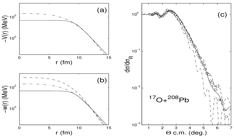
Figure 1: Optical potentials $V^{H}(V^{DF})+iW^{H}$, calculated in the microscopic approaches HEA(DF) for ${{}^{17}O}+{{}^{208}Pb}$ at $E_{l}=1435$ MeV; ${\it a}$ - real part of potentials, ${\it b}$ - imaginary part, ${\it c}$ - the ration of the respective elastic to the Rutherford differential cross-sections. In windows ${\it a}$ and ${\it b}$ dashed curves show potentials $V^{H}$ $W^{H}$, dash-dotted lines - $V^{DF}$, solid curves - Woods-Saxon fitted potentials. In window ${\it c}$ showed cross-sections calculated in the high-energy approximation (HEA): dashed curve - for $V^{H}\,+\,iW^{H}$, dash-dotted - for $V^{DF}\,+\,iW^{H}$, solid line - for the fitted WS-potential. Open circles - experimental data from [16].

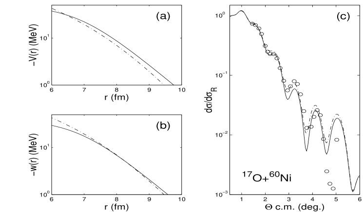
Figure 2: The case of scattering ${{}^{17}O}+{{}^{60}Ni}$ at 1435 MeV. In windows ${\it a}$ and ${\it b}$) are shown the microscopic optical potential $U^{C}_{opt}$ constructed from the real $V^{DF}$ and imaginary $V^{DF}$ patterns multiplied by the fitted factors $N_{r}$ and $N_{im}$ (dash-dotted curves); solid curves are the fitted WS-potentials. The respective differential cross-sections (window ${\it c}$), calculated in the HEA method. Solid curves are cross-sections for the Woods-Saxon potential fitted with experimental data [16] (”pseudo-experimental data”), dash-dotted curve is the cross-section for $U^{C}_{opt}$. The values of $N_{r}$ and $N_{im}$ see in Table 1.

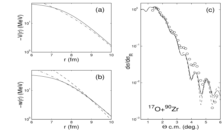
Figure 3: The same as in Fig.2 but for scattering ${{}^{17}O}+{{}^{90}Zr}$. In addition, dotted curves correspond to the $U^{B}_{opt}$ optical potential, composed from $V^{DF}$ and $W^{H}$ parts.

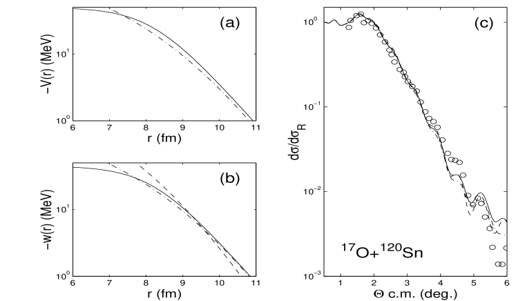
Figure 4: The same as in Fig.3 but for scattering ${{}^{17}O}+{{}^{120}Sn}$.

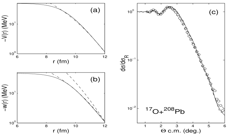
Figure 5: The same as in Fig.3 but for scattering ${{}^{17}O}+{{}^{208}Pb}$.

References

-
[1]
V.K.Lukyanov, E.V.Zemlyanaya, B.Słowiński, K.Hanna, Izv.RAN, ser.fiz.,
67, no.1, 55 (2003) (in Russian);
K.M.Hanna, V.K.Lukyanov, B.Słowiński, E.V.Zemlyanaya, Proc.Nucl.Part.Phys. Conf.(NUPPAC’01), Cairo, Egypt (2001) (ed.by M.N.H.Comsan and K.M.Hanna, printed in Cairo, 2002), p.121. - [2] R.J.Glauber, Lectures in Theoretical Physics (N.Y.: Interscience, 1959. P.315).
- [3] A.G.Sitenko, Ukr.Fiz.Zhurn.4, 152 (1959) (in Russian).
- [4] W.Czyz, L.C.Maximon, Ann.of Phys.(N.Y.) 52, 59 (1969).
- [5] J.Formanek, Nucl.Phys.B 12, 441 (1969).
- [6] V.K.Lukyanov, E.V.Zemlyanaya, J.Phys.G 26, 357 (2000).
- [7] P.Shukla, Phys.Rev.C 67, 054607 (2003).
- [8] V.K.Lukyanov, E.V.Zemlyanaya, K.V.Lukyanov, P4-2004-115, JINR, Dubna, 2004.
- [9] G.R.Satchler G.R. and W.G.Love, Phys.Rep. 55, 183 (1979).
-
[10]
V.K.Lukyanov, E.V.Zemlyanaya, B.Słowiński, Yad.Fiz. 67, 1306 (2004)
(in Russian);
V.K.Lukyanov, E.V.Zemlyanaya, B.Słowiński, Phys.Atom.Nucl. 67, 1282 (2004). - [11] Dao Tien Khoa, . .Knyaz’kov, Phys.El.Part.Nucl. 27, 1456 (1990).
- [12] D.T.Khoa, G.R.Satchler, Nucl.Phys.A 668, 3 (2000).
- [13] J.H.Sørensen and A.Winther, Nucl.Phys.A 550, 329 (1992).
- [14] Mervat H.Simbel, Phys.Rev.C. 56, 1467 (1997).
- [15] V.K.Lukyanov, E.V.Zemlyanaya, Int.J.Mod.Phys.E 10, 169 (2001).
- [16] R.Liguori Neto, P.Roussel-Chomaz, L.Rochais et al, Nucl.Phys.A 560, 733 (1993).
- [17] J.D.Patterson, R.J.Peterson, Nucl.Phys.A 717, 235 (2003).
- [18] M.El-Azab Farid and G.R.Satchler, Nucl.Phys.A 438, 525 (1985).
- [19] S.K.Charagi and S.K.Gupta, Phys.Rev.C. 41, 1610 (1990).
- [20] P.Shukla, arXiv:nucl-th/0112039.
- [21] D.T.Khoa, G.R.Satchler, W.von Oertsen, Phys.Rev.C 56, 954 (1997).