A Padé-aided analysis
of nonperturbative scattering in channel
Abstract
We carried out a Padé approximant analysis on a compact factor of the -matrix for scattering to explore the nonperturbative renormalization prescription in a universal manner. The utilities and virtues for this Padé analysis were discussed.
I Introduction
Since Weinberg’s seminal workWeinEFT , the effective field theory (EFT) approach to the nuclear forces has been extensively investigatedBevK . However, such applications are plagued by severe nonperturbative UV divergence. For the EFT approach to be useful, the regularization and subtraction scheme must be carefully worked out together with a consistent set of power counting rules. In other words, appropriate renormalization prescription is needed in nonperturbative regimes. There have been many contributions to this issuevK ; Epel ; Steele ; Rho ; KSW ; Fred ; Gege ; Soto ; BBSvK ; RGE ; Oller ; Nieves ; VA ; Higa (More could be found in Ref.BevK ), among which there are some controversies and debates. At some points, different approaches could lead to rather disparate predictionschLnforce .
Recently, a compact parametrization of the -matrix is proposed in Ref.g_npt , with which the obstacle for renormalization being identified as the compact form of the -matrix. In a concrete examplecontact , it was shown that the -matrix could only be renormalized through ’endogenous’ counter terms, which result in nontrivial prescription dependence. Such prescription dependence must be removed or fixed by imposing appropriate physical boundary conditions, for instance, through certain procedure of data fitting, as is frequently done in literature. The conventional power counting could be preserved within such procedures.
In this short report, we sketch a Padé approximant analysis basing on the aforementioned parametrization for the -matrix. The paper is organized as follows: In Sec. II, the parametrization proposed in Re.fg_npt is briefly described with some related remarks. In Sec. III, the Padé approximant of a factor in the compact parametrization of the -matrix is employed to parametrize the nonperturbative prescription dependence. Then predictions for phase shifts are made at various chiral orders and Padé approximants. The instrumental utilities and other aspects of this analysis will be discussed in Sec. IV. The report is summarized in Sec. IV.
II The compact parametrization
To describe low energy scattering, one first constructs the potential from PTWeinEFT up to certain chiral order, then computes the -matrix through Lippmann-Schwinger equation (LSE), which is plagued with severe nonperturbative UV divergences. To appreciate the crucial aspects, a compact form of -matrix in diagonal channelsfoot is proposed in Ref.g_npt as follows basing on LSE,
| (1) | |||
| (2) |
Here , with being nucleon mass, and being the off-shell external momenta. Using the on-shell relation between - and -matrixnewton : , we arrive at the following on-shell relations (from now on, we omit the subscript ’’)
| (3) | |||||
| (4) |
Obviously, assumes all the nonperturbative divergences in a compact form. Any approximation to the quantity leads to a nonperturbative scheme for . Here we should remind that the power counting is applied in the construction of the potential .
In perturbation theory, UV divergences are removed order by order before the amplitudes are summed up. While for Eq.(1) or (10) in nonperturbative regime, infinitely many UV divergent amplitudes like must be lump summed into a compact form. Then one must specify the order for implementing the following two incommutable procedures: subtraction versus nonperturbative summation. So a natural discrimination arises between ’endogenous’ and ’exogenous’ counter terms (or equivalent operations) that are introduced before and after the summation respectivelyg_npt ; contact . The compact form of -matrix fails the ’exogenous’ counter termsg_npt ; contact . In other words, the renormalization through ’endogenous’ counter terms is the only sensible procedure in nonperturbative regime. Since the Schrödinger equation approachBBSvK is intrinsically nonperturbative, any successful subtraction in the Schrödinger equation approach serves as a concrete instance for ’endogenous’ renormalization in actiong_npt ; contact . In practice, ’endogenous’ subtraction is a formidable task in the -matrix formalism: To complete the subtraction AND summation to ALL orders! That is why various forms of finite cutoff prevail in literature. In whatever approaches, the compact form of -matrix persists and makes nonperturbative prescription dependence strikingly different from the perturbative casesscheme ; contact : Physical boundary conditions must be imposed as a nontrivial procedure.
In what follows, all the EFT couplings are collectively denoted by and pion mass by . In general, any prescription could be parametrized by a set of dimensionless constants and a dimensional scale , including various finite cutoff schemes.
III a Padé-aided analysis of the EFT for scattering
III.1 Motivation
From the above discussions, it is clear that the nonperturbative renormalization prescription is solely assumed in the factor . Obviously, the factor could not be perturbative in terms of the EFT couplings, and its nontrivial nonperturbative prescription dependence is parametrized by the parameters to be physically fixed. These points have been demonstrated in Ref.contact . From the point of view of Eq.(1), the main issue in the EFT for low energy scattering is to work out an appropriate procedure or prescription of renormalization in the nonperturbative regime so that the EFT power counting schemes (encoded in ) remain intact. This requires the full solution of the nonperturbative factor .
Now we need a general formalism to describe the nontrivial features of the renormalization in the nonperturbative regimes. Due to the difficulty in obtaining the full analytical nonperturbative solutions, certain approximation must be employed in practice, including various numerical approachesEpel . Here, we wish to propose an approximation approach that is, we feel, more analytical in the nonperturbative regime. The starting point is just the compact parametrization defined in Eq.(1). We should note that in this parametrization the direct EFT component is the potential, which is constructed using EFT power counting. Thus the EFT is naturally incorporated in the following analysis through the potential. We will return to this issue in the third subsection.
III.2 Formulation
The idea is very simple, we parametrize the factor in terms of Padé approximant. This is reasonable as is nonperturbative in terms of the EFT couplings and prescription parameters. In formulae, we employ the following parametrization of the factor ():
| (5) |
Here, the Taylor series is also listed as an expansion in much lower energy regions. Note the significant distinction between the Padé analysis of the factor here and that of the whole -matrix: In the former case, EFT is indispensable in the systematic construction of the kernel (potential), while in the latter case, EFT plays no role at all.
Obviously assumes all the prescription dependence through or that are nontrivial functions of the EFT couplings , and the prescription parameters, . Then instead of , we could use or to parametrize the renormalization prescription of the -matrix within the EFT approach,
| (6) |
or
| (7) |
Intuitively, nonperturbative prescription dependence in or could be understood from the rigorous nonperturbative solution of on-shell -matrix for channel scattering with contact potential at next-to-leading order (Nlo) and next-to-next-to-leading order (Nnlo)contact :
| (8) | |||||
| (9) |
with , which correspond to , being polynomials in terms of coupling and . Here the constants come from divergent loop integrals and hence parametrize the renormalization prescription, like the set contact . Then effectively parametrize a prescription due to their nontrivial dependence on . In Padé approximant, or take over the role of , and the physical boundary conditions are to be imposed on or .
III.3 Power counting and nonperturbative prescription
As is stressed in the previous section, EFT and its power counting rules enter through the potential. Through Eq.(1) the EFT elements and their power counting rules are carried over to the -matrix in a nonperturbative manner. Since the kernel of the LSE or the potential is perturbative, its renormalization is still perturbatively implementable within the EFT power counting rules. Therefore, for the -matrix, Eq.(1) just provides a concise separation of the nonperturbative renormalization information from other things. Both and are in principle EFT objects, the sole and important distinction is that the former exclusively carries the information about the nonperturbative renormalization prescription. Thus, we could append some subscripts to Eq.(1) as follows,
| (10) |
In general, within a natural EFT, the nonperturbative objects (e.g. ) should also exhibit certain degree of naturalness in the sense that, the scales involved in such objects should not deviate very much from the natural sizes. But the renormalization in nonperturbative regimes does allow for other unconventional scenarios, without violating natural power counting rulescontact . As a matter of fact, the Padé analysis of alone according to Eq.(1) does not affect anything of the EFT power counting rules, i.e., the implementation of the EFT power counting rules and the nonperturbative renormalization procedures are disentangled. The possible subtleness in the nonperturbative factor should not be misunderstood as the inconsistency or the unnaturalness of the EFT power counting rules or even as the inapplicability of EFT method at all. That is, the unnaturalness in or could have nothing to do with the inconsistency of EFT power counting.
III.4 Fitting and predictions: channel
With the preceding preparations, we can demonstrate the predictions of phase shifts for the channel scattering at different orders of potential using different Padé approximants. For each case, the prescription parameters, i.e., the Padé parameters are fixed through fitting the phase shifts in the low energy ends. The laborious loop integrations and ’endogenous’ subtractions are naturally avoided.
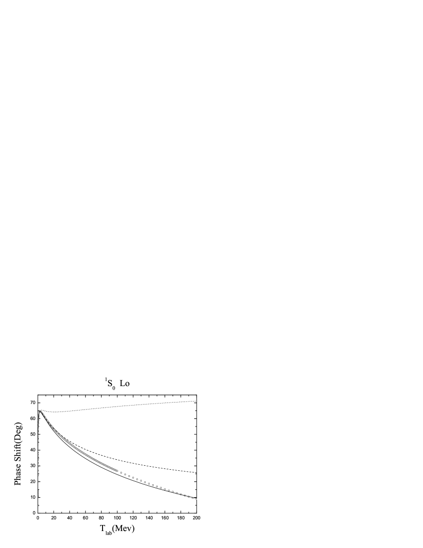
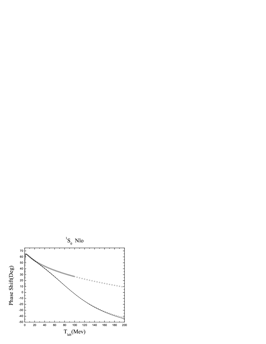
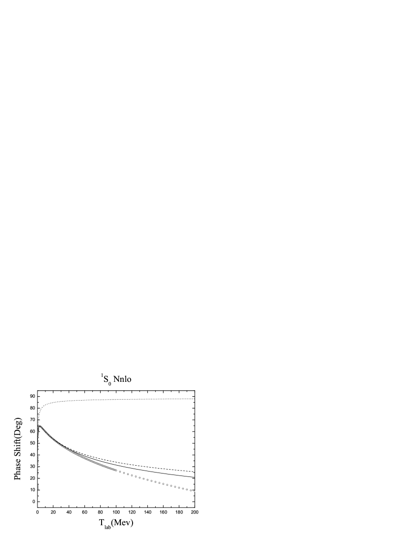
We will employ the potentials that are worked out in Ref.Epel (denoted as EGM from now on), which contains no energy dependence, and less contact couplings–a favorable aspect for fitting the ’physical’ values for or . One could well employ other construction schemes for potentials. In fact, one could compare any pair of potential schemes only through fitting the parameters or . It is obvious that at any chiral order with any Padé approximant, different Padé parameters would yield rather different phase shifts curves. We will not show the figures for demonstrating such nontrivial prescription dependence due to space limitation. Let us focus on more interesting figures with the Padé parameters determined through boundary conditions: fitting in the low energy regions: (1) At Lo, in units of MeV;(2) At Nlo , while ; (3) At Nnlo, . The phase shift is obtained from the following formula,
| (11) |
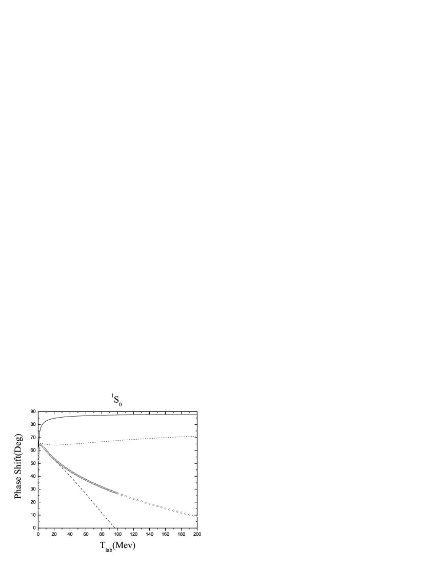
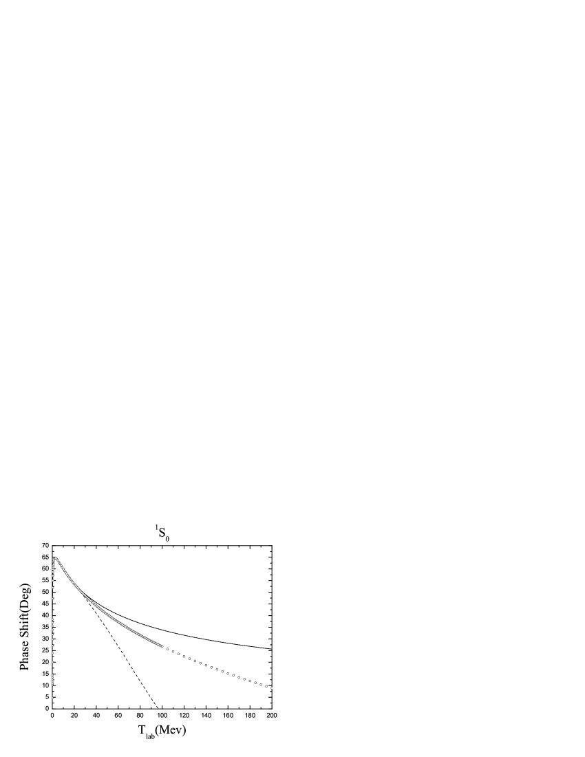
The phase shifts predicted at Lo, Nlo and Nnlo are depicted in Fig.1 (a), (b), (c) respectively. At each order, three Padé approximants are shown respectively: (1) (dotted lines); (2) (dashed lines); (3) (solid lines). From these diagrams, one could find that, at each order, the prediction improves as more Padé parameters are present, which is a natural tendency. One could also anticipate that with each Padé approximant, the predictions should also improve as higher order terms are present in the potential, which are responsible for the interactions at higher energy. The results are shown in Fig.2. In each figure, the predictions are compared among different orders of potential with a fixed Padé approximant. Note that in Fig.2 (b), in the whole range of the figure, the Lo curve almost identically coincides with the Nnlo curve.
Globally, the improvement with chiral orders is obvious: Nnlo prediction (solid line) is better than Nlo prediction (dashed line), and Nlo prediction is better than Lo (dotted line). There are also some interesting details: From these figures, we could see that in the higher energy region, all the Nlo curves have larger deviation from PWA data than the Nnlo curves. Some times, they are even worse than the Lo curves (C.f. Fig.2 (b) and (c)).
Here, we note that the solid curve in Fig.1 (a) seems puzzling. With only leading order potential ( plus a contact term ), one obtains pretty good predictions for the phase shifts, especially at the higher energies. The reason lies in the Padé approximant of , ), which is fixed ’physically’ and effectively ’induces’ higher order interactions upon iteration. This result agrees with the findings in Ref.Nieves , where a nonperturbative of -matrix is obtained using a simple potential (, and the prediction of the phase shifts is surprisingly good in a wider range of energy after the nonperturbative divergences is removed through fitting. Our analysis above provides a simple explanation of this surprise: The nonperturbative renormalization is properly treated! A closer look at the lower energy regions reveals that the higher order predictions still dominate the lower order ones (Cf. Fig.2 (c)). Generally, the lower order predictions could ’win’ at higher energies only by chance.
IV Utilities of Padé approximant and discussions
Now we have seen that after the nonperturbative prescription dependence is properly resolved (here realized through low energy region fitting), the EFT approach facilitates ’physical’ prediction for low energy scattering, at least in channel. Since no specification of regularization and renormalization is needed, the Padé approximant of defined in Eq.(1) in fact provides a universal parametrization of the renormalization prescription dependence of the -matrix in nonperturbative regimes. Note that both the potential and the Padé approximant of could be systematically extended to higher orders in EFT.
Comparing with previous results, we find that the Lo prediction with (C.f, Fig.2 (c)) differs significantly from that given in Ref.Epel and looks better. This nontrivial difference in predictions at leading order reflects the importance of nonperturbative renormalization. However, at higher chiral orders, especially at Nnlo, our results show no obvious differences in comparison with Ref.Epel . That means, including higher order interactions would lessen or tend to remove the nontrivial nonperturbative renormalization prescription dependence. This is a marvellous fact, since the fundamental requisite in EFT application is that renormalization prescription dependence should decrease as higher order interactions are included. Therefore, in spite of being an approximation approach, the procedures described above substantially proved or ascertained the rationality and applicability of EFT method in nuclear forces in a very general context. This is in sheer contrast to most known approaches where a renormalization prescription must be specified and hence the exploration of the prescription dependence is apparently limited.
So far we determined the Padé parameters through fitting with the potential defined by EGMEpel where the contact couplings were determined within a special cutoff scheme. In principle, we should determine the couplings in a way that is more prescription-independent: fitting through the combined space , which should lead to a better way for determining the EFT couplings. Now the Padé approximant provides us a convenient approach to do so without really carrying out the formidable task of loop integrations and renormalization to all orders. We will perform the investigations along this line in the future. We believe other utilities could be derived from this analysis and the parametrization Eq.(1).
From the above results, it is also obvious that it is fairly sufficient to employ Padé up to . For some channels, say -wave, it is often sufficient to use , which will be demonstrated in a separate report.
V summary
In summary, we performed a Padé analysis on a compact factor of the -matrix for scattering so that the nonperturbative prescription dependence and related effects could be conveniently explored. Such analysis suggests a useful theoretical instrument as well as a general and prescription-independent approach to test the efficiency and rationality of the application of EFT methods in nonperturbative regimes. Some related literature were also explained and discussed in favor of our analysis.
Acknowledgement
The authors are grateful to Dr. E. Epelbaum for helpful communications. JFY is grateful to Professor B. A. Kniehl for his hospitality at the II. Institute for Theoretical Physics of Hamburg University where part of this work was done. This project is supported in part by the National Natural Science Foundation under Grant No. 10205004.
References
- (1) S. Weinberg, Phys. Lett. B 251, 288 (1990); Nucl. Phys. B 363, 1 (1991).
- (2) See, e.g., P. Bedaque and U. van Kolck, Ann. Rev. Nucl. Part. Sci. 52, 339 (2002) [nucl-th/0203055]; Ulf-G. Meissner, nucl-th/0409028.
- (3) C. Ordóñez, L. Ray and U. van Kolck, Phys. Rev. C53, 2086 (1996); U. van Kolck, Nucl. Phys. A645, 327 (1999).
- (4) E. Epelbaum, W. Glöckle and U. Meissner, Nucl. Phys. A671, 295 (2000), Eur. Phys. J. A15, 543 (2002), A19, 125,401 (2004).
- (5) J.V. Steele and R.J. Furnstahl, Nucl. Phys. A637, 46 (1999).
- (6) T.S. Park, K. Kubodera, D.P. Min and M. Rho, Phys. Rev. C58, R637 (1998).
- (7) D.B. Kaplan, M.J. Savage and M.B. Wise, Phys. Lett. B424, 390 (1998); Nucl. Phys. B534, 329 (1998); S. Fleming, T. Mehen and I.W. Stewart, Nucl. Phys. A677, 313 (2000); Phys. Rev. C61, 044005 (2000).
- (8) T. Frederico, V.S. Timóteo and L. Tomio, Nucl. Phys. A653, 209 (1999).
- (9) J. Gegelia, Phys. Lett. B463, 133 (1999); J. Gegelia and G. Japaridze, Phys. Lett. B517, 476 (2001); J. Gegelia and S. Scherer, nucl-th/0403052.
- (10) D. Eiras and J. Soto, Eur. Phys. J. A17, 89 (2003)[nucl-th/0107009].
- (11) S.R. Beane, P. Bedaque, M.J. Savage and U. van Kolck, Nucl. Phys. A700, 377 (2002).
- (12) T. Barford and M.C. Birse, Phys. Rev. C67, 064006 (2003).
- (13) J.A. Oller, arXiv:nucl-th/0207086.
- (14) J. Nieves, Phys. Lett. B568, 109 (2003)[nucl-th/0301080].
- (15) M.P. Valderrama and E. Ruiz Arriola, Phys. Lett. B580, 149 (2004); Phys. Rev.C70, 044006 (2004).
- (16) R. Higa, nucl-th/0411046.
- (17) S.R. Beane and M.J. Savage, Nucl. Phys. A713, 148 (2003); Nucl. Phys. A717, 91 (2003); E. Epelbaum, W. Glöckle and U.-G. Meissner, Nucl. Phys. A714, 535 (2003).
- (18) J.-F. Yang, nucl-th/0310048v6(nucl-th/0407090).
- (19) J.-F. Yang and J.-H. Huang, Phys. Rev. C71, 034001(2005), ibid., C71, 069901(E) (2005)[nucl-th/0409023v3].
- (20) The generalization to the coupled channels is straightforward. We will perform such analysis in the coupled channels in the future.
- (21) R.G. Newton, Scattering Theory of Waves and Particles, 2nd Edition (Springer-Verlag, New York, 1982), p187.
- (22) P.M. Stevenson, Phys. Rev. D23, 2916 (1981); G. Grunberg, Phys. Rev. D29, 2315 (1984); S.J. Brodsky, G. P. Lepage and P. B. Mackenzie, Phys. Rev. D28, 228 (1983).
- (23) V.G.J. Stoks, R.A.M. Klomp, M.C.M. Rentmeester, and J.J. de Swart, Phys. Rev. C48, 792 (1993).
|
|
|
|---|---|---|
| (a) | (b) | (c) |
|
|

|
|---|---|---|
| (a) | (b) | (c) |