Collective dynamics of the fireball

Abstract

I analyse the identified single-particle $p_{t}$ spectra and two-pion Bose-Einstein correlations from RHIC. They indicate a massive transverse expansion and rather short lifetime of the system. The quantitative analysis in framework of the blast-wave model yields, however, unphysical results and suggests that the model may not be applicable in description of two-particle correlations. I then discuss generalisations of the blast-wave model to non-central collisions and the question how spatial asymmetry can be disentangled from flow asymmetry in measurements of $v_{2}$ and azimuthally sensitive HBT radii.

1 INTRODUCTION

When studying nuclear collisions at highest energies we are interested in properties of strongly interacting matter. A clear signal of existence of an extended piece of matter is its collective expansion which is not present in simple nucleon-nucleon collisions. This can be deduced from the slopes of identified hadronic single-particle $p_{t}$ spectra: while the slope is universal for all particle species in proton-proton collisions, the spectra become flatter with increasing particle mass in collisions of heavy ions.

Hadrons interact strongly an so they can only decouple from the system when it becomes dilute enough. Their spectra are fixed at the moment of freeze-out and carry information about the phase-space distribution in the final state of the fireball. We want to reconstruct this information and get an idea about the collective evolution of the fireball by comparing its final state to its initial state which is known from the energy and the collision geometry.

The process of freeze-out is very complicated [1]. Here I will simplify it and assume that all particles decouple along a specified three-dimensional freeze-out hypersurface [2]. The phase-space distribution at the freeze-out hypersurface will be parametrised by the so-called blast-wave model.

I will first introduce the model and analyse single-particle $p_{t}$ spectra and two-pion correlations from RHIC. Then I show how the model is generalised to non-central collisions and focus on calculation of $v_{2}$ and azimuthal dependence of HBT radii.

2 THE BLAST-WAVE MODEL FOR CENTRAL COLLISIONS

I will assume that in the end of its evolution the fireball is in a state of local thermal equilibrium given by temperature $T$ and chemical potentials $\mu_{i}$ for every species $i$. The freeze-out hypersurface will stretch along the $\tau=\sqrt{\rm{t}^{2}-\rm{z}^{2}}=\tau_{0}=\mbox{const}$ hyperbola and will not depend on the transverse radial coordinate $r$. There is longitudinally boost-invariant expansion, i.e. $v_{z}=z/t$. The velocity field

$$u^{\mu}=(\cosh\rho\,\cosh\eta,\,\cos\psi\,\sinh\rho,\,\sin\psi\,\sinh\rho,\,\cosh\rho\,\sinh\eta)\,.$$ (1)

Here, $\rho$ stands for the transverse rapidity which will be assumed to depend linearly on $r$

$$\rho=\rho_{0}{r}/{R}\,.$$ (2)

Note that this linear dependence was found for small transverse velocities also in hydrodynamic simulations [3]. In the last equation, $R$ is the transverse size of the fireball. The transverse density distribution is uniform for $r<R$. The (Wigner) phase-space distribution of particles at freeze-out is then characterised by the emission function

$$S(x,p)\,d^{4}x = \frac{m_{t}\,\cosh(y-\eta)}{(2\pi)^{3}}\,\left[\exp\left(\frac{p\cdot u-\mu}{T}\right)\pm 1\right]^{-1}\theta(R-r)$$ (3)

$$r\,dr\,d\psi\,d\eta\,\frac{\tau\,d\tau}{\sqrt{2\pi\,\Delta\tau^{2}}}\exp\left(-\frac{(\tau-\tau_{0})^{2}}{2\,\Delta\tau^{2}}\right)\,,$$

where the term $m_{t}\,\cosh(y-\eta)$ comes from the Cooper-Frye pre-factor $d\sigma^{\mu}p_{\mu}$ [2] and the exponential in $\tau$ represents smearing in the freeze-out time. The energy in the statistical distribution is taken in the rest-frame of the fluid: $E=p\cdot u$. This introduces “coupling” between momentum of the emitted particle and the flow velocity of the piece of fireball where it comes from. The strength of this coupling is controlled by $1/T$.

2.1 Calculation of spectra

The single-particle spectrum is obtained from the correlation function as

$$E\frac{d^{3}N}{dp^{3}}=\int d^{4}x\,S(x,p)\,.$$ (4)

For low $p_{t}$, the inverse slope of the spectrum is roughly given by [4]

$$T_{*}=T+m\langle v_{t}\rangle^{2}\,.$$ (5)

Here, $\langle v_{t}^{2}\rangle$ is the mean transverse collective expansion velocity. Thus the freeze-out temperature and the transverse expansion cannot be both determined from a measurement of only one single-particle spectrum. However, they can be determined from identified spectra of different species.

The full expression for the single-particle spectrum reads [5]

$$E\frac{d^{3}N}{dp^{3}} = \frac{1}{2\pi^{2}}\int_{0}^{\infty}dr\,r\,G(r)\,\tau_{0}(r)\,\Bigg{\{}m_{t}\,K_{1}\left(\frac{m_{t}\cosh(\rho(r))}{T}\right)I_{0}\left(\frac{p_{t}\sinh(\rho(r))}{T}\right)$$ (6)

$$\qquad\qquad\qquad\qquad{}-p_{t}\frac{d\tau_{0}}{dr}\,K_{0}\left(\frac{m_{t}\cosh(\rho(r))}{T}\right)I_{1}\left(\frac{p_{t}\sinh(\rho(r))}{T}\right)\Bigg{\}}\,.$$

Note that in the model given by emission function eq. (3), $G(r)=\theta(R-r)$ and the second term vanishes because $d\tau_{0}/dr=0$. Here I display a more general expression because I want to discuss all effects which influence the single-particle spectrum:

1. Freeze-out temperature and the transverse expansion velocity.

2. Contributions to particle production from resonance decays. This is not included in the formula (6) but is important in particular for pion production (and will be included in calculations below). In this connection also chemical potentials of the individual resonance species are important as they determine the number of resonances and thus the fraction of pions which stem from their decays.

3. The shape of freeze-out hypersurface enters through the term $d\tau_{0}/dr$.

4. Also “finer details” like the profile $G(r)$, spatial dependence of the temperature, the radial profile of the transverse velocity, etc. can influence the spectrum [4, 6].

It is important to realise that two models which differ in points 2–4 may not give the same $T$ and $\langle v_{t}\rangle$ when fitted to single-particle spectra. For example, in the single-freeze-out model [7] $\tau_{0}=\sqrt{\mbox{const}+\rm{z}^{2}+r^{2}}$ and the second term on the r.h.s. of eq. (6) gives a contribution. Thus the temperature obtained from fits with that model cannot be directly compared to the one which will obtained below [8].

2.2 Calculation of HBT radii

I will also calculate the HBT radii in Bertsch-Pratt parametrisation (see e.g. [9] for more details on HBT interferometry). They appear as width parameters of a Gaussian parametrisation of the correlation function

$$C(q,K)-1=\lambda\exp\left(-R_{o}^{2}(K)q_{o}^{2}-R_{s}^{2}(K)q_{s}^{2}-R_{l}^{2}(K)q_{l}^{2}\right)\,,$$ (7)

where $q$ and $K$ are momentum difference and the average momentum of the pair, respectively, and the $R$’s are the HBT radii. They measure the lengths of homogeneity [10], i.e., sizes of the part of the source which produces pions with specified momentum. The sizes are measured in three directions: longitudinal is parallel to the beam, outward parallel to transverse component of $K$, and sideward is the remaining Cartesian direction. The parametrisation (7) is valid in the CMS frame at mid-rapidity of central collisions; otherwise terms mixing two components of $q$ may appear (like $R_{ol}^{2}q_{o}q_{l}$, for example; see [9] for more details). The HBT radii will be determined as

$$R_{o}^{2}(K) = \langle(\tilde{\rm}{x}-\beta_{t}\tilde{\rm}{t})^{2}\rangle\,,$$ (8a)

$$R_{s}^{2}(K) = \langle\tilde{\rm}{y}^{2}\rangle\,,$$ (8b)

$$R_{l}^{2}(K) = \langle\tilde{\rm}{z}^{2}\rangle\,.$$ (8c)

In eqs. (8) $\rm{x}$, $\rm{y}$, $\rm{z}$, $\rm{t}$ stand for the Cartesian space-time coordinates, $\rm{z}$ is the longitudinal coordinate and $\rm{x}$ the outward coordinate. Averaging and the tilde are defined as

$$\langle f(x)\rangle(K)=\frac{\int d^{4}x\,f(x)\,S(x,K)}{\int d^{4}x\,S(x,K)}\,,\qquad\tilde{x}^{\mu}=x^{\mu}-\langle x^{\mu}\rangle\,,\qquad\beta_{t}=\frac{K_{t}}{K^{0}}\,.$$ (9)

Because the lengths of homogeneity depend on momentum, the HBT radii show dependence on $K_{t}$. For $R_{s}^{2}(K_{t})$, an approximate formula says [4]

$$R_{s}^{2}=\frac{R_{G}^{2}}{1+\rho_{0}M_{t}/T}\,\qquad\mbox{with}\quad M_{t}=\sqrt{m^{2}+K_{t}^{2}}\,.$$ (10)

Thus the temperature $T$ and transverse expansion measured by $\rho_{0}$ are coupled together here. However, recalling eq. (5), they can be disentangled by analysing both the HBT radii and the single particle $m_{t}$ spectrum.

3 THE FREEZE-OUT STATE IN CENTRAL COLLISIONS

I will fit the model to single-particle spectra and HBT radii measured at RHIC. First, each of the identified spectra of pions, kaons, and protons of both charges will be fitted individually. This provides a consistency check for the assumption that all these species freeze-out simultaneously: if the results of the fits are incompatible, this assumption is invalid. After that, I will fit the HBT radii and look again whether they can be accommodated with the same model as the single-particle spectra.

Resonance production of pions will be taken into account for spectra but not for HBT radii. A study of the influence of resonance production on HBT radii indicated that in the presence of transverse flow they are changed only marginally [11].

Chemical potentials of the resonance species are determined in accord with the model of partially chemically frozen gas [12]. It assumes that after the chemical freeze-out [13] the effective numbers of particles decaying weakly (and thus slowly) stay fixed while the strong (and therefore fast) interactions stay in equilibrium. Effective number of any given species includes this species plus particles which can be produced on average from decays of all present resonances. Adjectives “fast” and “slow” refer to comparison with the typical time scale of the fireball evolution. As an example: effective number of pions $\tilde{N}_{\pi}=N_{\pi}+2N_{\rho}+N_{\Delta}+\dots$, and chemical potential of $\Delta$ will be $\mu_{\Delta}=\mu_{\pi}+\mu_{N}$ because it is in equilibrium with pions and nucleons.

Au+Au at $\sqrt{s}=130\,A\mbox{GeV}$. When fitting the various single-particle spectra [14], no overlap of the fit results is found at 1$\sigma$ level. The $\chi^{2}$ contours in freeze-out temperature $T$ and the average transverse expansion velocity $\langle v_{t}\rangle$ are overlapping at 95% confidence level at $T\approx 120-140\,\mbox{MeV}$ and $\langle v_{t}\rangle\approx 0.45-0.5$.

Figure 1: Two fits to the HBT radii measured in Au+Au collisions at $\sqrt{s}=130A\mbox{GeV}$. Dashed lines show a fit with values that also reproduce the single-particle spectra: $T=121\,\mbox{MeV}$, $\langle v_{t}\rangle=0.51$, $R=12.1\,\mbox{fm}$, $\tau_{0}=4.3\,\mbox{fm}/c$, $\Delta\tau=4.4\,\mbox{fm}/c$. Solid lines show the best fit to $\pi^{+}\pi^{+}$ correlations: $T=33\,\mbox{MeV}$, $\langle v_{t}\rangle=0.73$, $R=24.1\,\mbox{fm}$, $\tau_{0}=21.3\,\mbox{fm}/c$, $\Delta\tau=1.1\,\mbox{fm}/c$.

Can we fit the HBT radii with these values? In Figure 1 I plot the HBT radii measured by STAR [15] and PHENIX [16] collaborations together with two fits. It turns out that $R_{s}(K_{t})$ is so steep that—within this model—it rules out the temperatures obtained from spectra analysis. A lower temperature is favoured, the best fit being obtained for $T=33\,\mbox{MeV}$! But this is not the freeze-out temperature! The unphysically low value of the parameter $T$ just indicates that in order to reproduce the observed strong $K_{t}$ dependence of HBT radii the coupling of momentum to the local flow velocity in the emission function eq. (3) must be very strong.

Figure 2: Fits to the HBT radii measured in Au+Au collisions at $\sqrt{s}=200A\mbox{GeV}$. Preliminary data are read off the figures presented at the Quark Matter 2002 conference [19, 20]. Dashed lines show a fit with values that also reproduce the single-particle spectra: $T=115\,\mbox{MeV}$, $\langle v_{t}\rangle=0.57$, $R=13.3\,\mbox{fm}$, $\tau_{0}=4.7\,\mbox{fm}/c$, $\Delta\tau=4.7\,\mbox{fm}/c$. Solid lines show the best fit to the HBT radii: $T=28\,\mbox{MeV}$, $\langle v_{t}\rangle=0.71$, $R=27.7\,\mbox{fm}$, $\tau_{0}=24.9\,\mbox{fm}/c$, $\Delta\tau=1.7\,\mbox{fm}/c$.

Au+Au at $\sqrt{s}=200\,A\mbox{GeV}$. Results from fits to identified single-particle spectra of pions, kaons and protons [17, 18] overlap at 1$\sigma$ level at $T\approx 115\,\mbox{MeV}$ and $\langle v_{t}\rangle\approx 0.57$. The fit to HBT radii (Fig. 2) with these parameters is marginally good. The best fit is again obtained with an unphysically low freeze-out temperature. The distinguishing power between the two models will be improved when final data will be fitted. Note that a fit to final results from PHENIX seem to be in better agreement with the conventional parameter values [21].

A very low freeze-out temperature is also obtained when the complete collection of HBT radii form Pb+Pb collisions at projectile energy of 158 $A$GeV is fitted. That fit is not shown here due to lack of space.

Conclusions from central collisions. The parameters obtained in the fits to $K_{t}$ dependence of HBT radii have no direct physics interpretation. The low temperature just indicates the need for very strong coupling between momentum and flow within the blast-wave model. The model seems not to describe the realised scenario of freeze-out.

In spite of all these failures, one has to notice that the measured $R_{s}$, which is the rms radius of the source, indicates a strong transverse expansion since the original rms radius of Au nucleus is about 3.5 fm. If we model the nucleus and the fireball by a box-like transverse distribution, this is an expansion from a radius of $~{}7\,\mbox{fm}$ to about 12 fm (in the “conventional” models with $T\approx 100-120\,\mbox{MeV}$). The total lifetime in Bjorken longitudinal expansion scenario can be estimated from $\tau_{0}+\Delta\tau\approx 9\,\mbox{fm}/c$. It remains puzzling how the fireball expands transversely so much in such a short time without any original transverse flow.

4 NON-CENTRAL COLLISIONS

Next I generalise the model for non-central collisions. The transverse profile becomes ellipsoidal instead of circular, so this changes the $\theta$-function from eq. (3) into

$$\theta(R-r)\to\theta\left(R-R\sqrt{\frac{\rm{x}^{2}}{R_{x}^{2}}+\frac{\rm{y}^{2}}{R_{y}^{2}}}\right)\,,\qquad R_{x}=a\,R\,,\qquad R_{y}=R/a\,.$$ (11)

Here I define the direction of the $\rm{x}$-coordinate to be parallel to the impact parameter, and $\rm{y}$-coordinate as perpendicular to the reaction plane. The spatial anisotropy is parametrised by the parameter $a$. The transverse flow rapidity—given by eq. (2) for central collisions—will also vary with the angle $\psi$ with respect to the reaction plane

$$\rho(r,\psi)=\frac{r}{R}\sqrt{a^{-2}\cos^{2}\psi+a^{2}\sin^{2}\psi}\,\rho_{0}\,\left(1+\rho_{2}\cos(2\psi_{\textrm{flow}})\right)\,.$$ (12)

I will discuss two models which differ in the azimuthal dependence of $\rho(r,\psi)$ [22].
Model 1: Transverse velocity is perpendicular to the surface and $\psi_{\textrm{flow}}=\mbox{Arctan}\frac{\rm{y}}{\rm{x}}$ [23].
Model 2: Transverse velocity points outwards in radial direction, $\psi_{\textrm{flow}}=\psi$.

4.1 Elliptic flow coefficient $v_{2}$

Elliptic flow can be generated by two different mechanisms in our model. Firstly, the fireball can be spatially ellipsoidal, but have the same transverse velocity at the outer shell. Secondly, the fireball can have spatially circular cross-section, but the expansion velocity can be higher in one direction than in the other. It would be interesting to disentangle these two effects from the data. For example, if we can learn about the shape of the fireball, we obtain an indirect information about the lifetime because the fireball starts as out-of-plane elongated and via expansion this shape becomes more and more circular. An out-of-plane elongated (i.e. $a<1$) fireball at freeze-out is thus an indication of short lifetime.

The coefficient $v_{2}$ can be calculated in both used models; it turns out that the results obtained for Model 1 map exactly to those for Model 2 if one replaces $a\to 1/a$ [22]. Hence, without the knowledge about which model applies better for the description of the freeze-out, one cannot say anything about whether the fireball is in-plane or out-of-plane elongated at freeze-out just by looking at $v_{2}$. If the model is fixed, $v_{2}$ depends on $a$ and $\rho_{2}$ in a different way for different species, so one should be able to disentangle them from a measurement of $v_{2}(p_{t})$ of more than one identified species.

4.2 Azimuthally sensitive HBT

Since the HBT radii are measured along directions specified by the orientation of the transverse momentum, they depend explicitly on the angle $\phi$ between the transverse momentum and the reaction plane. In addition to that, homogeneity regions depend on the momentum of produced particles and this introduces an implicit azimuthal dependence. (See [9] for more on azimuthal dependence of HBT radii.)

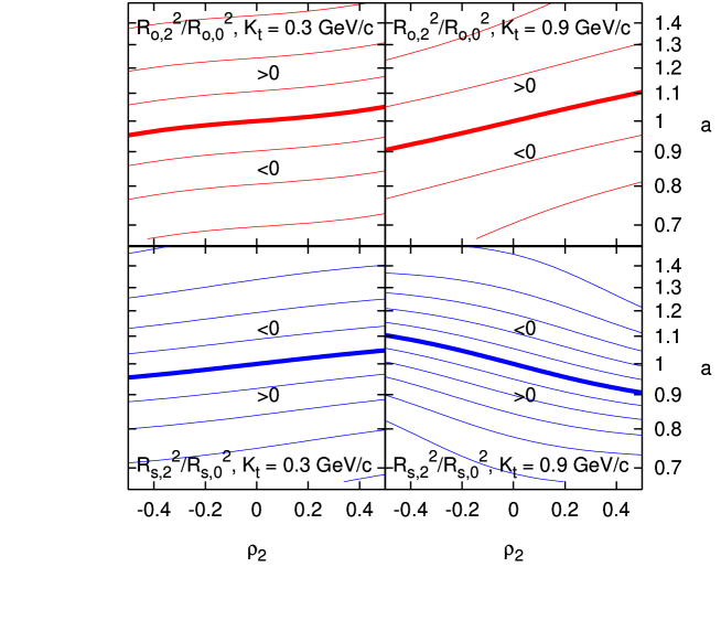
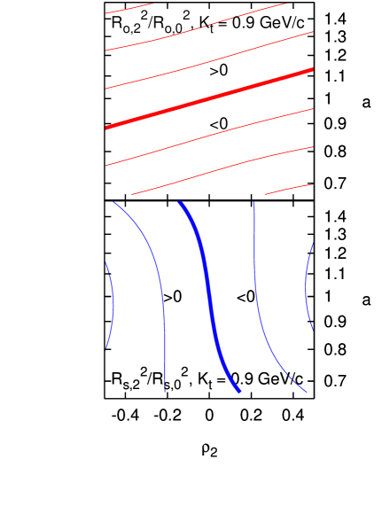
Figure 3: The second order Fourier terms normalised by the average HBT radii $R_{i,2}^{2}/R_{i,0}^{2}$ (see eq. (13)) as a function of $a$ and $\rho_{2}$. Upper row: outward radius; lower row: sideward radius. Thick lines show where there is no second-order oscillation of the radius as a function of $\phi$. Consecutive lines correspond to increments by 0.1. Left panel: calculation with Model 1 at $p_{t}=300\,\mbox{MeV}/c$ (left) and $p_{t}=900\,\mbox{MeV}/c$ (right). Right panel: calculation with Model 2 at $p_{t}=900\,\mbox{MeV}/c$; results at $p_{t}=300\,\mbox{MeV}/c$ are similar to Model 1.

One quantifies the azimuthal dependence of HBT radii by decomposing them into Fourier series. Up to leading oscillating terms this reads

$$\begin{array}[]{ll}R_{o}^{2}(\phi)=R_{o,0}^{2}+2R_{o,2}^{2}\cos(2\phi)+\dots\,,&\qquad R_{s}^{2}(\phi)=R_{s,0}^{2}+2R_{s,2}^{2}\cos(2\phi)+\dots\,,\\ R_{os}^{2}(\phi)=2R_{os,2}^{2}\sin(2\phi)+\dots\,,&\qquad R_{l}^{2}(\phi)=R_{l,0}^{2}+2R_{l,2}^{2}\cos(2\phi)+\dots\,.\end{array}$$ (13)

We will be interested in the dependence of second-order amplitude of the outward radius $R_{o,2}^{2}$ and the sideward radius $R_{s,2}^{2}$ on the spatial anisotropy $a$ and flow anisotropy $\rho_{2}$. We would like to eliminate their scaling with the absolute transverse size of the fireball, so we will divide them by the respective average terms $R_{i,0}^{2}$.

This is plotted in Figure 3. The good news from this figure is that almost in all cases the normalised oscillation amplitude $R_{i,2}^{2}/R_{i,0}^{2}$ depends mainly on spatial anisotropy and only weakly on flow anisotropy. The only found exception is $R_{s}^{2}$ in Model 2: its oscillation is dictated by flow asymmetry at high $p_{t}$. At low $p_{t}$, the homogeneity regions are mainly characterised by the shape of the fireball. At higher $p_{t}$, they become more sensitive to the flow. In case of Model 2 this can even lead to a change of sign of the amplitude $R_{s,2}^{2}$ [22].

4.3 Comparison with data

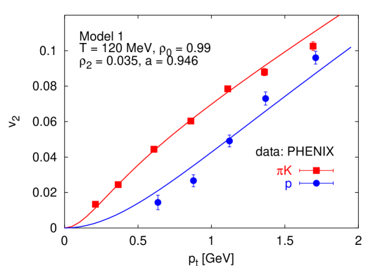
Figure 4: Elliptic flow coefficient $v_{2}$ measured by the PHENIX collaboration in Au+Au collisions at $\sqrt{s}=200~{}A\mbox{GeV}$ for the centrality class 20–30% [24] as a function of $p_{t}$ for a pions and kaons (squares) and for identified protons (circles). Theoretical curves are obtained with the Model 1 using parameter values indicated in the figure.

Figure 5: Azimuthal dependence of the HBT radii at midrapidity from Au+Au collisions at 200 $A$GeV and centrality class 20–30% measured by the STAR Collaboration [25]. From highest till lowest the data are taken for $K_{t}$ values: 0.2, 0.3, 0.4, and 0.52 GeV/$c$. Theoretical curves are calculated with Model 1 with the parameter values: $T=120\,\mbox{MeV}$, $\rho_{0}=0.99$, $\rho_{2}=0.035$, $a=0.94646$, $R=9.4\,\mbox{fm}$, $\tau_{0}=5.0\,\mbox{fm}/c$, $\Delta\tau=2.9\,\mbox{fm}/c$.

By comparing to data one can try to distinguish whether we observe an in-plane or out-of-plane elongated fireball and which of the two introduced models is better. In Figure 4 I show $v_{2}(p_{t})$ compared to curves calculated with Model 1. Within this model we obtain an out-of-plane elongated source ($a<1$), i.e., a source which remembers its original deformation. Recall, however, that the same theoretical curves can be obtained in Model 2 if we change $a$ into $1/a$, so we would have an in-plane elongated source.

The key to resolve this ambiguity is a fit to the data on azimuthal dependence of HBT radii. I can fit their oscillation well with Model 1 if I assume parameters from the fit to $v_{2}$; this is shown in Figure 5. I checked that in Model 2 the amplitude of oscillations is opposite to what the data show [22]. The conclusion is that the observed fireball is out-of-plane elongated and that Model 1 reproduces data better than Model 2.

With the used “conventional” values of temperature and average radial flow gradient $\rho_{0}$ I could not reproduce the absolute size and $K_{t}$ dependence of the sideward HBT radius, but note that this is the same kind of problems as was observed in central collisions.

5 CONCLUSIONS

We do see a strong collective transverse expansion at RHIC (and at SPS) because the transverse size of the source is much larger than the original nuclei. The total lifetime seems to be short: this is indicated by the size of $R_{l}$ when interpreted in Bjorken scenario and by the fact that in non-central collisions we observe an out-of-plane elongated source so there wasn’t enough time to wash away this anisotropy. On the other hand, the lifetime must also be long enough to allow the fireball for a massive transverse expansion. This, together with the failure of the blast-wave model in fitting the HBT radii, indicates that the model does not provide a satisfactory description of the decoupling of particles. As the freeze-out temperature is always obtained in a specific model there is no conclusion about its particular value.

References

- [1] V. Magas, these proceedings.
- [2] F. Cooper and G. Frye, Phys. Rev. D 10 (1974) 186.
- [3] P. F. Kolb, arXiv:nucl-th/0304036.
- [4] T. Csörgő and B. Lörstad, Phys. Rev. C 54 (1996) 1390.
- [5] E. Schnedermann, J. Sollfrank and U. Heinz, Phys. Rev. C 48, 2462 (1993).
- [6] B. Tomášik and U. Heinz, Eur. Phys. J. C 4 (1998) 327.
- [7] W. Broniowski and W. Florkowski, Phys. Rev. Lett. 87 (2001) 272302.
- [8] U. Heinz, talk at the RIKEN BNL Workshop, Nov. 17-19, 2003, http://tonic.physics.sunysb.edu/flow03/.
- [9] B. Tomášik and U.A. Wiedemann, in Quark-Gluon Plasma 3, R.C. Hwa and X.-N. Wang eds., World Scientific, 2003, hep-ph/0210250.
- [10] A.N. Makhlin and Y.M. Sinyukov, Z. Phys. C 39 (1988) 69.
- [11] U.A. Wiedemann and U.W. Heinz, Phys. Rev. C 56 (1997) 3265.
- [12] H. Bebie, P. Gerber, J.L. Goity and H. Leutwyler, Nucl. Phys. B 378 (1992) 95.
- [13] P. Braun-Munzinger, D. Magestro, K. Redlich and J. Stachel, Phys. Lett. B 518 (2001) 41.
- [14] K. Adcox et al. [PHENIX Collaboration], Phys. Rev. Lett. 88 (2002) 242301.
- [15] C. Adler et al. [STAR Collaboration], Phys. Rev. Lett. 87 (2001) 082301.
- [16] K. Adcox et al. [PHENIX Collaboration], Phys. Rev. Lett. 88 (2002) 192302.
- [17] J. Adams et al [STAR Collaboration], Phys. Rev. Lett. 92 (2004) 11230.
- [18] S.S. Adler et al. [PHENIX Collaboration], Phys. Rev. C 69 (2004) 034909.
- [19] M. López Noriega for the STAR Collaboration, Nucl. Phys. A715 (2003) 623c.
- [20] A. Enokizono for the PHENIX Collaboration, Nucl. Phys. A715 (2003) 595c.
- [21] F. Retière, J. Phys. G 30 (2004) S827.
- [22] B. Tomášik, arXiv:nucl-th/0409074.
- [23] F. Retière and M.A. Lisa, arXiv:nucl-th/0312024.
- [24] S.S. Adler et al. [PHENIX Collaboration], Phys. Rev. Lett. 91 (2003) 182301.
- [25] J. Adams et al [STAR Collaboration], Phys. Rev. Lett. 93 (2004) 012301.