Disentangling Spatial and Flow Anisotropy

Abstract

Two generalisations of the blast-wave model to non-central nuclear collisions are constructed, and elliptic flow as well as azimuthal dependence of correlation radii are calculated. Particular attention is paid to how different azimuthal dependences of transverse flow direction can cause qualitatively different anisotropic fireballs to give same $v_{2}$ as a function of the transverse momentum. The simultaneous dependence of $v_{2}$ and the oscillation of correlation radii on both spatial and flow anisotropy is studied in great detail.

1 Introduction

The so-called “elliptic flow” $v_{2}$ [1], observed in non-central nuclear collisions at highest available energies [2, 3], has had important implications on understanding of the collision dynamics in framework of hydrodynamic and cascade models [4, 5]. After exclusion of non-flow effects the “elliptic flow” can be caused by azimuthal anisotropy in transverse expansion and/or anisotropic shape of the fireball. It was noticed that it was not possible to conclude on the spatial anisotropy of the freeze-out state simply from data on $v_{2}$. However, a conjecture [6] was made that measurements of HBT correlation radii as functions of azimuthal angle [7] will give access to the spatial shape of the fireball. Indeed, this was observed [8] in hydrodynamic simulations with two different sets of initial conditions: they lead to different final states which could have been distinguished by pion interferometry.

This paper focuses in great detail on the question to what extent the spatial shape and the anisotropy of transverse flow can be identified from data. In contrast to hydrodynamic simulations where given model and initial conditions lead to a single freeze-out state, parameterisations of the final state will be employed here. These parameterisations, which will be constructed by generalising the blast-wave model [9], allow to investigate a broad range of various freeze-out states and find their possible signatures in the data. A much more systematic study than in a hydrodynamic simulation is thus possible; the price to pay is that no connection to fireball evolution is made.

The generalisation of the blast-wave model to non-central collisions is not unique. In order to explore possible ambiguities due to various angular dependences of the expansion velocity, I will study two models.

There is a correlation between the spatial and the flow anisotropy in determining $v_{2}$; same $v_{2}$ can be caused by many different combinations of the two anisotropies. This correlation depends on the mass of particles but—unfortunately—it also depends crucially on the used model. Thus the flow anisotropy cannot be disentangled from the spatial anisotropy unless the model is known. On the other hand, irrespective the model, the azimuthal dependence of correlation radii seems to be mostly sensitive to the spatial anisotropy, at least in the low-$p_{t}$ region.

First, in the next Section I will introduce a generalised blast-wave model. Then, $v_{2}$ (Section 3) and correlation radii (Section 4) are calculated and their dependence on spatial and flow anisotropy is studied. Technical details concerning the calculations can be found in Appendices.

2 A generalisation of the blast-wave model

This generalisation follows mainly ref. [10] with some variations in introducing the azimuthal dependence of the transverse velocity. (Experts in the field can skip most of this section and look just at the introduction of two different azimuthal dependences of the transverse flow velocity, after eq. (10).)

It is assumed that at the end of its evolution the fireball is in a state of local thermal equilibrium characterised by a temperature $T$. Decoupling of particles is (almost) instantaneous and can be modelled by the Cooper-Frye formalism [11] along a freeze-out hyper-surface.

The time of freeze-out does not depend on position in direction transverse to the beam, only the longitudinal coordinate matters. Motivated by the Bjorken boost-invariant longitudinal expansion [12], the freeze-out hyper-surface is given by a hyperbola

$$\tau_{0}=\sqrt{{\rm t}^{2}-{\rm z}^{2}}=\mbox{const}\,,$$ (1)

where ${\rm t}$ and ${\rm z}$ are temporal and longitudinal coordinate, respectively. We will allow for some smearing of the freeze-out time $\tau_{0}$ by amount $\Delta\tau$.

We assume that the decoupling matter is distributed uniformly and the transverse cross-section has ellipsoidal shape. Thus the density will be proportional to $\Theta(1-\tilde{r})$ where

$$\tilde{r}=\sqrt{\frac{{\rm x}^{2}}{R_{x}^{2}}+\frac{{\rm y}^{2}}{R_{y}^{2}}}\,.$$ (2)

In this equation, ${\rm x}$ and ${\rm y}$ are Cartesian coordinates in the direction of the impact parameter and perpendicular to the reaction plane, respectively. They can be rewritten with the help of the usual radial coordinates

$${\rm x} = r\,\cos\phi_{s}\,,$$ (3a)

$${\rm y} = r\,\sin\phi_{s}\,,$$ (3b)

(the reason for subscript “$s$” on the angular coordinate will become clear later). The radii $R_{x}$ and $R_{y}$ in eq. (2) stand for the sizes in the corresponding directions. They will be expressed via the average radius $R$ and the spatial anisotropy parameter $a$

$$R_{x}=a\,R\,,\qquad R_{y}=R/a\,.$$ (4)

Thus a fireball elongated out of the reaction plane corresponds to $a<1$, while $a>1$ stands for an in-plane elongated source.

We do not assume any geometric limitation in the longitudinal direction, therefore the fireball is actually infinite in this direction. We can do this as we will be only interested in observables at mid-rapidity in collisions at very high energy (at RHIC e.g.) where boost invariance is locally established. The actual finiteness of the effective source is established dynamically [13]. Those parts of the fireball moving too fast forward or backward cannot emit mid-rapidity particles.

The source is modelled by an emission function. This is the Wigner phase space density of particle emission

$$S(x,p)\,d^{4}x=\frac{m_{t}\,\cosh(y-\eta)}{(2\pi)^{3}}\,d\eta\,d{\rm x}\,d{\rm y}\,\frac{\tau\,d\tau}{\sqrt{2\pi\,\Delta\tau}}\\ \times\exp\left(-\frac{(\tau-\tau_{0})^{2}}{2\,\Delta\tau^{2}}\right)\,\Theta(1-\tilde{r})\,\exp\left(-\frac{p^{\mu}u_{\mu}}{T}\right)\,.$$ (5)

Table 1: Summary of model parameters.

freeze-out temperature	$T$
average transverse flow gradient	$\rho_{0}$
variation of the flow gradient	$\rho_{2}$
average transverse radius	$R$
spatial anisotropy	$a$
mean Bjorken lifetime	$\tau_{0}$
freeze-out time dispersion	$\Delta\tau$

Here, we use space-time rapidity $\eta$ and longitudinal proper time $\tau$ instead of ${\rm t}$ and ${\rm z}$

$${\rm t} = \tau\,\cosh\eta\,,$$ (6a)

$${\rm z} = \tau\,\sinh\eta\,.$$ (6b)

Momentum $p$ will be parametrised in terms of rapidity $y$, transverse momentum $p_{t}$, transverse mass $m_{t}=\sqrt{m^{2}+p_{t}^{2}}$ and azimuthal angle $\phi$

$$p^{\mu}=(m_{t}\cosh y,\,p_{t}\cos\phi,\,p_{t}\sin\phi,\,m_{t}\sinh y)\,.$$ (7)

The term $m_{t}\cosh(y-\eta)$ in the emission function comes from the flux of particles through an infinitesimal piece of the freeze-out hyperbola: $p^{\mu}d\sigma_{\mu}$ [11]. In the Boltzmann distribution, energy is taken in the rest frame of the emitting piece of the fireball

$$E^{*}=p^{\mu}u_{\mu}(x)\,,$$ (8)

where $u_{\mu}$ is local collective velocity of the fireball. The use of Boltzmann distribution is justified as long as the temperature is not too low and the chemical potential (for pions) is small; here we put $\mu=0$.

Velocity field $u_{\mu}(x)$ describes the collective expansion of the fireball [9]. In longitudinal direction we assume a boost-invariant expansion which is given by

$$v_{z}=\tanh\eta\,.$$ (9)

The transverse velocity will be parametrised with the help of transverse rapidity $\rho$

$$v_{\perp}=\tanh\rho\,.$$ (10)

Rapidity $\rho$ will depend on the position in the transverse plane. We will consider two models which will differ in the azimuthal variation of the transverse velocity.

Model 1. In this model transverse expansion velocity is always directed perpendicularly to the surface given by $\tilde{r}=\mbox{const}$ [10]. Its angle with respect to the reaction plane is thus

$$\phi_{b}=\mbox{Arctan}\frac{{\rm y}}{{\rm x}}$$ (11)

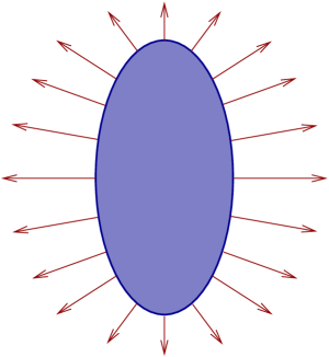
Model 1

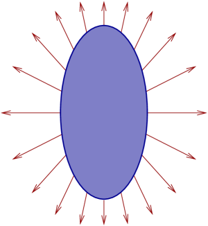
Model 2

Figure 1: Two used models of azimuthal variation of the transverse flow velocity. The depicted anisotropies correspond to $a<1$ and $\rho_{2}>0$.

(see Figure 1). Note that

$$\tan\phi_{b}=\left(\frac{R_{x}}{R_{y}}\right)^{2}\tan\phi_{s}=a^{4}\tan\phi_{s}\,.$$ (12)

The magnitude of the transverse rapidity also varies with $\phi_{b}$

$$\rho=\tilde{r}\,\rho_{0}(1+\rho_{2}\cos(2\phi_{b}))\,,$$ (13)

where $\rho_{0}$ and $\rho_{2}$ are tunable parameters. (Note the slight difference to the parametrisation of Retière and Lisa [10] who write $\rho=\tilde{r}(\rho_{0}+\rho_{2}\cos(2\phi_{b}))$.)

The velocity field $u^{\mu}(x)$ is then written as

$$u^{\mu}=(\cosh\rho\,\cosh\eta,\,\cos\phi_{b}\,\sinh\rho,\,\sin\phi_{b}\,\sinh\rho,\,\cosh\rho\,\sinh\eta)\,.$$ (14)

Later in the calculation it will be convenient to use coordinates $\tilde{r}$ and $\phi_{b}$ in the transverse plane instead of ${\rm x}$ and ${\rm y}$. It is shown in Appendix A that

$$d{\rm x}\,d{\rm y} = J_{1}(\phi_{b})\,R^{2}\,\tilde{r}\,d\tilde{r}\,d\phi_{b}\,,$$ (15a)

$$J_{1}(\phi_{b}) = (a^{2}\cos^{2}\phi_{b}+a^{-2}\sin^{2}\phi_{b})^{-1}\,.$$ (15b)

Model 2. Here it will be assumed that the transverse velocity is always directed radially. Then the angle between transverse velocity and the reaction plane coincides with $\phi_{s}$ (see eq. (3)). Transverse rapidity will be given by

$$\rho=\tilde{r}\,\rho_{0}(1+\rho_{2}\cos(2\phi_{s}))\,.$$ (16)

The difference to Model 1 is in the use of $\phi_{s}$ instead of $\phi_{b}$, cf. equation (13). The velocity field is similar to eq. (14), except for the replacement $\phi_{b}\to\phi_{s}$

$$u^{\mu}=(\cosh\rho\,\cosh\eta,\,\cos\phi_{s}\,\sinh\rho,\,\sin\phi_{s}\,\sinh\rho,\,\cosh\rho\,\sinh\eta)\,.$$ (17)

In this case, the appropriate coordinates to use are $\tilde{r}$ and $\phi_{s}$. The Jacobian is calculated in Appendix A

$$d{\rm x}\,d{\rm y} = J_{2}(\phi_{s})\,R^{2}\,\tilde{r}\,d\tilde{r}\,d\phi_{s}$$ (18a)

$$J_{2}(\phi_{s}) = (a^{-2}\cos^{2}\phi_{s}+a^{2}\sin^{2}\phi_{s})^{-1}\,.$$ (18b)

All parameters of the models are summarised in Table 1.

3 Elliptic flow

The elliptic flow coefficient $v_{2}$ is introduced through the Fourier decomposition of the azimuthal dependence of single-particle spectrum [1]. At mid-rapidity in symmetric collision systems such a decomposition includes only even cosine terms

$$P_{1}(p_{t},\phi) = \left.\frac{d^{3}N}{p_{t}\,dp_{t}\,dy\,d\phi}\right|_{y=0}$$ (19)

$$= \frac{1}{2\pi}\,\left.\frac{d^{2}N}{p_{t}\,dp_{t}\,dy}\right|_{y=0}\,\left(1+2v_{2}(p_{t})\cos(2\phi)+\dots\right)\,.$$

In this formulation, $\phi$ is the angle between the transverse momentum and the reaction plane. The coefficient $v_{2}$ can thus be calculated as

$$v_{2}(p_{t})=\frac{\int_{0}^{2\pi}P_{1}(p_{t},\phi)\,\cos(2\phi)\,d\phi}{\int_{0}^{2\pi}P_{1}(p_{t},\phi)\,d\phi}\,.$$ (20)

Single-particle spectrum is obtained from the emission function by integrating over the space-time

$$P_{1}(p_{t},\phi)=\int d^{4}x\,S(x,p)\,.$$ (21)

Combining eqs. (20) and (21) we obtain expressions for $v_{2}$ in our models; see Appendix B for details of the calculation. For Model 1 (velocity perpendicular to the surface) we obtain

$$v_{2}=\frac{\int_{0}^{1}d\tilde{r}\,\tilde{r}\int_{0}^{2\pi}d\phi_{b}\,\cos(2\phi_{b})\,J_{1}(\phi_{b})\,\mbox{K}_{1}\left(\frac{m_{t}\cosh\rho(\tilde{r},\phi_{b})}{T}\right)\mbox{I}_{2}\left(\frac{p_{t}\sinh\rho(\tilde{r},\phi_{b})}{T}\right)}{\int_{0}^{1}d\tilde{r}\,\tilde{r}\int_{0}^{2\pi}d\phi_{b}\,J_{1}(\phi_{b})\,\mbox{K}_{1}\left(\frac{m_{t}\cosh\rho(\tilde{r},\phi_{b})}{T}\right)\mbox{I}_{0}\left(\frac{p_{t}\sinh\rho(\tilde{r},\phi_{b})}{T}\right)}\,\\ \mbox{[Model 1]}$$ (22)

while for Model 2 (radially directed transverse velocity) we have

$$v_{2}=\frac{\int_{0}^{1}d\tilde{r}\,\tilde{r}\int_{0}^{2\pi}d\phi_{s}\,\cos(2\phi_{s})\,J_{2}(\phi_{s})\,\mbox{K}_{1}\left(\frac{m_{t}\cosh\rho(\tilde{r},\phi_{s})}{T}\right)\mbox{I}_{2}\left(\frac{p_{t}\sinh\rho(\tilde{r},\phi_{s})}{T}\right)}{\int_{0}^{1}d\tilde{r}\,\tilde{r}\int_{0}^{2\pi}d\phi_{s}\,J_{2}(\phi_{s})\,\mbox{K}_{1}\left(\frac{m_{t}\cosh\rho(\tilde{r},\phi_{s})}{T}\right)\mbox{I}_{0}\left(\frac{p_{t}\sinh\rho(\tilde{r},\phi_{s})}{T}\right)}\,\\ \mbox{[Model 2]}$$ (23)

where $\mbox{K}_{1}$, $\mbox{I}_{0}$, and $\mbox{I}_{2}$ are modified Bessel functions. Since we integrate over the angle, the only difference between the two results is in the use of the Jacobian terms $J_{1}$ or $J_{2}$. Moreover, the difference between these two terms is only in the replacement $a\to a^{-1}$. As the anisotropy parameter $a$ does not appear anywhere else in relations (22) and (23), any $v_{2}$ calculated in one model is equal to $v_{2}$ calculated in the other model under transformation $a\to a^{-1}$. Thus we have an analytic example of two models which lead to the same $v_{2}$, while one is elongated in-plane and the other out-of-plane. This clearly demonstrates that there is no possibility to distinguish in-plane source from out-of-plane source just by measuring $v_{2}$.

Physics reason behind the observation that the two models are “inverse” to each other can be deduced from Figure 1. The arrows denote expansion velocity and their lengths indicate its magnitude. Both situations in that Figure correspond to $\rho_{2}>0$ and $a<1$. In case of Model 1, most arrows point rather in the reaction plane (which is taken to be horizontal in this Figure), so the major boost effect leading to enhancement of the spectrum happens in this direction. For Model 2, a larger part of the flow is directed out of the reaction plane and the enhancement of spectra due to the boost is in that direction. Thus Model 1 would lead to positive $v_{2}$ while Model 2—in this setup—to negative $v_{2}$. This is, of course, just a qualitative argument. The equivalence of the two models under replacement $a\to a^{-1}$ is derived analytically.

We can therefore calculate $v_{2}$ just for one of the models; results for the second one are then obtained trivially. I will choose Model 1.

Dependence of $v_{2}$ on the transverse momentum and particle identity in Model 1 was thoroughly studied in [10]. In the data [2, 3] for small $p_{t}$, $v_{2}$ is positive, increases with increasing $p_{t}$ and decreases with growing mass of particles. This behaviour is reproduced in Model 1 if $a<1$ and $\rho_{2}>0$. (Loosely speaking, one of these conditions may be broken, but not “too much”; see later when the results are shown.) In this parameter region, calculation shows that $v_{2}$ of heavier particles can become negative at low $p_{t}$ and start growing and be positive above some value of $p_{t}$ [10, 14]. Such a dip to negative $v_{2}$ is also observed by STAR Collaboration for antiprotons in certain centrality bins [3], but the effect may not be statistically significant.

We will be interested in how the spatial and the flow anisotropies are entangled in determining $v_{2}$ for various identified particle species.

In comparing $v_{2}$ of different species it turns out to be unwise to use the $p_{t}$-averaged $v_{2}$. This is because the averages are weighted with the single-particle spectra which are not alike for different species: those for heavier particles are flatter. Hence, averaging $v_{2}(p_{t})$ for heavy particles can sometimes lead to larger resulting values than the same procedure yields with light particles, although the value of $v_{2}$ at any $p_{t}$ is lower for heavy particles. The reason is that flatter spectrum for heavy particles gives stronger weight to larger $v_{2}$ at higher $p_{t}$.

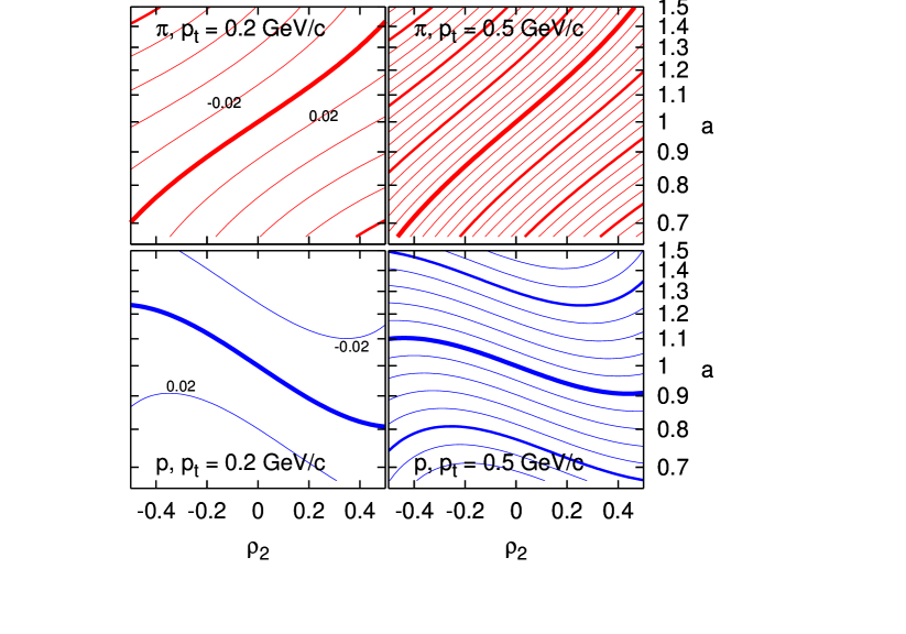
Figure 2: Contour plots of $v_{2}$ as a function of $a$ and $\rho_{2}$, calculated in Model 1 for $T=100\,\mbox{MeV}$ and $\rho_{0}=0.88$. Upper row: pions, lower row: protons. Left column: $p_{t}=200\,\mbox{MeV}/c$, right column: $p_{t}=500\,\mbox{MeV}/c$. The thickest lines show where $v_{2}$ vanishes. Consecutive lines correspond to increments/decrements by 0.02.

Therefore, we study the entanglement of $a$ and $\rho_{2}$ in determining $v_{2}$ for pions and protons at two fixed values of $p_{t}$. As can be seen from eqs. (22) and (23), $v_{2}$ does not depend on $R$, $\tau_{0}$ and $\Delta\tau$. Since the dependence on all other parameters was studied in detail in [10], here we just fix $T$ and $\rho_{0}$, and plot $v_{2}$ as a function of $a$ and $\rho_{2}$ in Figure 2. We clearly see how the two anisotropy parameters are correlated and that the correlation depends strongly on the type of particles. Recall that a figure for Model 2 would be obtained just by inverting the $a$-scale.

Temperature and radial flow can be roughly obtained from azimuthally integrated spectra which are weakly sensitive to $a$ and $\rho_{2}$ [10]. Then, if one was able to determine the correct model for the description of the freeze-out, spatial and flow anisotropy could be disentangled from measurements of $v_{2}$ as a function of $p_{t}$ for different identified particle species [3]. However, the choice of the model cannot be based on $v_{2}$ measurement.

4 Azimuthal angle dependence of correlation radii

In this section we focus on azimuthal angle dependence of correlation radii due to spatial and flow anisotropy. First, explicit and implicit $\phi$-dependences are discussed. Then, necessary formalism is introduced. Experts can skip this and proceed directly to Section 4.3 where the results are presented.

4.1 Explicit and implicit azimuthal angle dependence

In non-central collisions one can study Bose-Einstein correlations of identical pions for particles emitted under different azimuthal angles [7]. To start the argument, let us just take a single emitter which emits particles in all directions. The directions in which the sizes of the emitter are measured, are given by the momentum. Therefore, by changing azimuthal angle $\phi$ of the momentum, the correlation radii measure the size of the anisotropic source in different directions. This leads to explicit dependence of the correlation radii on $\phi$. (See below how correlation radii are defined.) The explicit azimuthal dependence is thus connected with the spatial anisotropy.

In a real case, we have an expanding fireball of which only a part—the homogeneity region—effectively produces particles with a given momentum [13]. Thus particles in different directions can be produced from different homogeneity regions which differ in sizes. This mechanism leads to an additional, so-called implicit azimuthal dependence of the correlation radii. It is intimately connected with transverse expansion and its anisotropy. Here we want to see how these two kinds of effects act together in azimuthally sensitive correlation studies.

4.2 Formalism

We will confine ourselves to theoretical calculations at mid-rapidity for symmetric collision systems. The reader is referred to [15, 16] for summary of the formalism of Bose-Einstein interferometry in non-central collisions.

Correlation radii are width parameters of a Gaussian parametrisation of the measured correlation function

$$C(q,K)=1+\lambda\,\exp(-R_{s}^{2}(K)q_{s}^{2}-R_{o}^{2}(K)q_{o}^{2}-R_{l}^{2}(K)q_{l}^{2}\\ {}-2R_{os}^{2}(K)q_{o}q_{s}-2R_{ol}^{2}(K)q_{o}q_{l}-2R_{sl}^{2}(K)q_{s}q_{l})\,$$ (24)

where the momenta of the pair have been parametrised in terms of

$$q = p_{1}-p_{2}$$ (25a)

$$K = \textstyle{\frac{1}{2}}(p_{1}+p_{2})$$ (25b)

and the phenomenological parameter $\lambda\leq 1$ is due to a variety of effects ranging from partial coherence of the source up till particle misidentification. The standard out-side-long coordinate system is used, with longitudinal axis in beam direction, outward axis parallel to the transverse component of $K$, and sideward direction perpendicular to the previous two. Correlation radii are given by sizes in these directions. Recall that in non-central collisions we identify the Cartesian x-y-z frame with the collision geometry: ${\rm z}$-axis points in beam direction, ${\rm x}$-axis is parallel to the impact parameter, and ${\rm y}$-axis is perpendicular to the reaction plane. Hence, there is an angle $\phi$ between the ${\rm x}$-axis and the outward direction and we are interested in the $\phi$-dependence of the correlation radii.

If there is no tilt of the fireball in the reaction plane [17], the two radii $R_{ol}^{2}$ and $R_{sl}^{2}$ vanish. This is the case with the used models. The remaining radii can be calculated as [7]

$$R_{s}^{2} = \textstyle{\frac{1}{2}}(\langle\tilde{\rm x}^{2}\rangle+\langle\tilde{\rm y}^{2}\rangle)-\textstyle{\frac{1}{2}}(\langle\tilde{{\rm y}}^{2}\rangle-\langle\tilde{{\rm x}}^{2}\rangle)\cos 2\phi-\langle\tilde{{\rm x}}\tilde{{\rm y}}\rangle\sin 2\phi\,,$$ (26a)

$$R_{o}^{2} = \textstyle{\frac{1}{2}}(\langle\tilde{\rm x}^{2}\rangle+\langle\tilde{\rm y}^{2}\rangle)+\textstyle{\frac{1}{2}}(\langle\tilde{{\rm y}}^{2}\rangle-\langle\tilde{{\rm x}}^{2}\rangle)\cos 2\phi+\langle\tilde{{\rm x}}\tilde{{\rm y}}\rangle\sin 2\phi$$ (26b)

$${}+\beta_{\perp}^{2}\langle\tilde{{\rm t}}^{2}\rangle\,-2\beta_{t}\langle\tilde{{\rm t}}\tilde{{\rm x}}\rangle\cos\phi-2\beta_{t}\langle\tilde{{\rm t}}\tilde{{\rm y}}\rangle\sin\phi\,,$$

$$R_{os}^{2} = \textstyle{\frac{1}{2}}(\langle\tilde{{\rm y}}^{2}\rangle-\langle\tilde{{\rm x}}^{2}\rangle)\sin 2\phi+\langle\tilde{{\rm x}}\tilde{{\rm y}}\rangle\cos 2\phi$$ (26c)

$${}+\beta_{t}\langle\tilde{{\rm t}}\tilde{{\rm x}}\rangle\sin\phi-\beta_{t}\langle\tilde{{\rm t}}\tilde{{\rm y}}\rangle\cos\phi\,,$$

$$R_{l}^{2} = \langle(\tilde{{\rm z}}-\beta_{l}\tilde{{\rm t}})^{2}\rangle\,,$$ (26d)

where

$$\langle f(x)\rangle(K) = \frac{\int f(x)\,S(x,K)\,d^{4}x}{\int S(x,K)\,d^{4}x}\,,$$ (27a)

$$\tilde{\rm x}^{\mu} = {\rm x}^{\mu}-\langle{\rm x}^{\mu}\rangle\,.$$ (27b)

The explicit azimuthal dependence is displayed in eqs. (26). In addition, the (co-)variances $\langle\tilde{\rm x}^{\mu}\tilde{\rm x}^{\nu}\rangle$ can depend on $\phi$ and this is the implicit azimuthal dependence. From eqs. (26), correlation radii can be calculated for both Models just by inserting the corresponding emission function.

Azimuthal dependence of the correlation radii can be analysed with the help of Fourier decomposition. Due to a number of symmetry arguments [16] in our setup, the relevant Fourier series, truncated after the leading oscillating terms, are

$$R_{o}^{2}(\phi) = R_{o,0}^{2}+2R_{o,2}^{2}\cos 2\phi+\dots$$ (28a)

$$R_{s}^{2}(\phi) = R_{s,0}^{2}+2R_{s,2}^{2}\cos 2\phi+\dots$$ (28b)

$$R_{os}^{2}(\phi) = 2R_{os,2}^{2}\sin 2\phi+\dots$$ (28c)

$$R_{l}^{2}(\phi) = R_{l,0}^{2}+2R_{l,2}^{2}\cos 2\phi+\dots\,.$$ (28d)

4.3 Results

We will focus on $R_{o}^{2}$ and $R_{s}^{2}$, as we are interested in anisotropies in the transverse plane. The absolute sizes of these radii together with their oscillation amplitudes scale with the total geometric size $R$. We can get rid of this scaling and thus observe the effect due to anisotropies more cleanly when we study the ratios $R_{o,2}^{2}/R_{o,0}^{2}$ and $R_{s,2}^{2}/R_{s,0}^{2}$ [10].

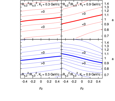
Model 1

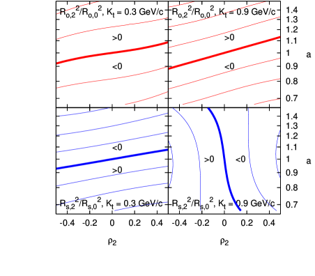
Model 2

Figure 3: Dependence of the normalised second order oscillation terms $R_{o,2}^{2}/R_{o,0}^{2}$ (upper rows) and $R_{s,2}^{2}/R_{s,0}^{2}$ (lower rows) on spatial anisotropy $a$ and flow anisotropy $\rho_{2}$, calculated for $K_{t}=300\,\mbox{MeV}/c$ (left columns) and $K_{t}=900\,\mbox{MeV}/c$ (right columns), with Model 1 (upper panel) and Model 2 (lower panel). Thick contour lines correspond to 0, consecutive curves to increments/decrements by 0.1. Other model parameters in the calculation were $T=0.1\,\mbox{GeV}$, $\rho_{0}=0.88$, $R=9.41\,\mbox{fm}$, $\tau_{0}=9\,\mbox{fm}/c$, and $\Delta\tau=1\,\mbox{fm}/c$.

These ratios for Model 1 and Model 2 are plotted in Figure 3. In most cases, oscillations of correlation radii are mainly determined by the spatial anisotropy and not so much by the flow anisotropy. The only exception is $R_{s}^{2}$ at high $p_{t}$ in Model 2: the $\phi$-dependence in this model changes from shape-determined to flow-determined, i.e. dominated by the implicit azimuthal dependence. In all other cases, $\phi$-dependence of the correlation radii follows the explicit azimuthal angle dependence rather well.

Figure 4: Azimuthal angle dependence of $R_{s}^{2}$ in Model 2 at various transverse momenta. Values of parameters used in the calculation: $T=0.1\,\mbox{GeV}$, $\rho_{0}=0.88$, $\rho_{2}=0.2$, $R=9.41\,\mbox{fm}$, $a=0.95$, $\tau_{0}=9\,\mbox{fm}/c$, and $\Delta\tau=1\,\mbox{fm}/c$. Different curves correspond from top to bottom to transverse momenta of 0.2, 0.4, 0.6, 0.8, and 1 GeV/$c$.

The behaviour of $R_{s}^{2}$ in Model 2 is shown in Figure 4. The azimuthal angle dependence changes qualitatively with increasing $p_{t}$: at the given parameter values oscillation amplitude is positive at low $p_{t}$ and becomes negative at large $p_{t}$.

Model 1

Model 2

Figure 5: Azimuthal angle dependence of correlation radii in Model 1 (left) and Model 2 (right) in comparison with data. Curves and data points correspond from top to bottom to transverse momenta of 0.2, 0.3, 0.4, and 0.52 GeV/$c$. Values of parameters used in the calculation are chosen such that $v_{2}(p_{t})$ is reproduced (not shown here, see [18]): $T=0.12\,\mbox{GeV}$, $\rho_{0}=0.99$, $\rho_{2}=0.035$, $R=9.41\,\mbox{fm}$, $\tau_{0}=5.02\,\mbox{fm}/c$, and $\Delta\tau=2.90\,\mbox{fm}/c$. Spatial anisotropies are $a=0.946$ (Model 1) or $a=1.057$ (Model 2). Data points are measured by the STAR collaboration [19] in 20-30% centrality events of Au+Au collisions at $\sqrt{s}=200\,A\mbox{GeV}$.

Now we come to the question if one of the models can be disqualified by comparing to data. In Figure 5 we see two models which reproduce $v_{2}$ quite well (this is shown in [18]); they are related by transformation $a\to a^{-1}$. However, since the oscillation of correlation radii is mostly shaped by the spatial anisotropy, the two models lead to opposite predictions of the sign of the oscillation amplitudes—and Model 2 is in qualitative disagreement with the data. I do not try to find the perfect fit here; this turns out to be a problematic task with the blast-wave model [20, 18]. Nonetheless, note that the qualitative features of the azimuthal angle dependence of the correlation radii are reproduced in Model 1 under the assumption of an out-of-plane extended source, which confirms the earlier conclusion of STAR [19]

5 Conclusions

Generalisation of the popular blast-wave model to non-central collisions is not unique. Many possible ways differ in how the transverse velocity depends on the azimuthal angle $\phi_{s}$.

In this paper two such generalisations were constructed. Then, a number of statements scattered in literature were demonstrated in a unified framework of a generalised blast-wave model, which is often used in many variations. The interplay of HBT analysis with $v_{2}$ for identified species should be stressed.

I showed analytically how two very different fireballs can lead to the same $v_{2}$, such that from measuring only this quantity one cannot conclude whether the source is elongated in-plane or out-of-plane [6].

The azimuthal angle dependence of the correlation radii, on the other hand, can be used for this. It is mostly sensitive at low $p_{t}$ to the spatial anisotropy of the fireball [8].

When the type of the model is identified from comparison to data on two-pion correlations, spatial and flow anisotropy can be disentangled from reproducing $v_{2}(p_{t})$ of different identified species and $\phi$-dependence of correlation radii. Before measuring anisotropies, temperature and radial flow can be determined from azimuthally integrated single-particle spectra which are nearly independent of the anisotropy parameters.

Among the two models used here, Model 2 fails qualitatively in reproducing data on azimuthal angle dependence of the correlation radii. In a simple qualitative comparison with the data, the other Model indicates that the observed fireball in non-central Au+Au collisions at $\sqrt{s}=200\,A\mbox{GeV}$ is elongated out of the reaction plane, in agreement with conclusions of [19].

Acknowledgements

I thank Evgeni Kolomeitsev, Mike Lisa, Scott Pratt, and Fabrice Retière for stimulating discussions.

This research was supported by a Marie Curie Intra-European Fellowship within the 6th European Community Framework Programme.

Appendix A Jacobians for integration in transverse plane

As it is simpler, we begin with the Model 2. The aim is to use $\tilde{r}$ and $\phi_{s}$ as coordinates in the transverse plane. Because

$${\rm x} = r\,\cos\phi_{s}$$ (29a)

$${\rm y} = r\,\sin\phi_{s}\,,$$ (29b)

we only have to replace $r$ by $\tilde{r}$. From eqs. (2) and (4) we obtain

$$\tilde{r}=\frac{r}{R}\sqrt{a^{-2}\cos^{2}\phi_{s}+a^{2}\sin^{2}\phi_{s}}\,.$$ (30)

This leads to

$${\rm x} = \frac{\tilde{r}\,R\,\cos\phi_{s}}{\sqrt{a^{-2}\cos^{2}\phi_{s}+a^{2}\sin^{2}\phi_{s}}}$$ (31a)

$${\rm y} = \frac{\tilde{r}\,R\,\sin\phi_{s}}{\sqrt{a^{-2}\cos^{2}\phi_{s}+a^{2}\sin^{2}\phi_{s}}}\,,$$ (31b)

and

$$d{\rm x}\,d{\rm y}=\frac{R^{2}\,\tilde{r}\,d\tilde{r}\,d\phi_{s}}{a^{-2}\cos^{2}\phi_{s}+a^{2}\sin^{2}\phi_{s}}\,.$$ (32)

Thus we derived eq. (18).

For the Model 1 we want to use the angle $\phi_{b}$ as a coordinate instead of $\phi_{s}$. By making use of eq. (12) we can rewrite eq. (31) into

$${\rm x} = \frac{\tilde{r}\,R\,\mbox{sgn}(\cos\phi_{s})}{\sqrt{a^{-2}+a^{2}\tan^{2}\phi_{s}}}$$ (33a)

$$= \frac{\tilde{r}\,R\,a^{2}\,\cos\phi_{b}}{\sqrt{a^{2}\cos^{2}\phi_{b}+a^{-2}\sin^{2}\phi_{b}}}$$

$${\rm y} = \frac{\tilde{r}\,R\,\mbox{sgn}(\sin\phi_{s})}{\sqrt{a^{-2}\mbox{cotan}^{2}\phi_{s}+a^{2}}}$$ (33b)

$$= \frac{\tilde{r}\,R\,a^{-2}\,\sin\phi_{b}}{\sqrt{a^{2}\cos^{2}\phi_{b}+a^{-2}\sin^{2}\phi_{b}}}\,.$$

In the last expression we introduced

$$\mbox{sgn}(x)=\Big{\{}\begin{array}[]{r@{\quad:\quad}l}+1&x\geq 0\\ -1&x<0\end{array}\,,$$

and exploited that

$$\mbox{sgn}(\sin\phi_{s}) = \mbox{sgn}(\sin\phi_{b})$$

$$\mbox{sgn}(\cos\phi_{s}) = \mbox{sgn}(\cos\phi_{b})\,.$$

From eqs. (33) it is straightforward to obtain the Jacobian for Model 1

$$d{\rm x}\,d{\rm y}=\frac{R^{2}\,\tilde{r}\,d\tilde{r}\,d\phi_{b}}{a^{2}\cos^{2}\phi_{b}+a^{-2}\sin^{2}\phi_{b}}\,.$$ (34)

Notice that apart from the use of $\phi_{b}$ instead of $\phi_{s}$, one obtains the Jacobian for Model 2 from that of Model 1 just by replacing $a\to a^{-1}$.

Appendix B Calculation of $v_{2}$

Let us calculate $v_{2}$ for Model 1. First, we need the azimuthally integrated single-particle spectrum in the denominator of eq. (20). From eqs. (7) and (14) we obtain that

$$p^{\mu}u_{\mu}=m_{t}\,\cosh(\eta-y)\,\cosh\rho(\tilde{r},\phi_{b})-p_{t}\,\sinh\rho(\tilde{r},\phi_{b})\,\cos(\phi-\phi_{b})\,.$$ (35)

This is the energy argument for the Boltzmann distribution. In accord with eqs. (21) and (5), azimuthally integrated spectrum is obtained as

$$\int_{0}^{2\pi}P_{1}(p_{t},\phi)\,d\phi\\ \,=\int_{0}^{2\pi}d\phi\int d^{4}x\,S(x,p)\\ \,=\int_{0}^{2\pi}d\phi\int_{0}^{2\pi}d\phi_{b}\,J_{1}(\phi_{b})\int_{0}^{1}d\tilde{r}\,\tilde{r}\,R^{2}\,\int_{-\infty}^{\infty}d\eta\,\frac{m_{t}\cosh(\eta-y)}{(2\pi)^{3}}\\ \quad\times\int_{-\infty}^{\infty}\frac{d\tau\,\tau}{\sqrt{2\pi\,\Delta\tau^{2}}}\,\exp\left(-\frac{(\tau-\tau_{0})^{2}}{2\,\Delta\tau^{2}}\right)\\ \quad\times\exp\left(-\frac{m_{t}\,\cosh(\eta-y)\,\cosh\rho(\tilde{r},\phi_{b})-p_{t}\,\sinh\rho(\tilde{r},\phi_{b})\,\cos(\phi-\phi_{b})}{T}\right)$$ (36)

where $J_{1}(\phi_{b})$ was defined in eq. (15). The integration over $\tau$ is trivial. We are interested in mid-rapidity particles in the centre-of-mass frame, so $y=0$. Then, integration over $\eta$ can be performed and leads to the modified Bessel function $\mbox{K}_{1}$ [21]. We can exchange the order of integrations in $\phi$ and $\phi_{b}$, and perform a transformation $\phi\to\phi-\phi_{b}=\psi$. The integral in $\psi$ can then be performed analytically and leads to the modified Bessel function $\mbox{I}_{0}$. We finally arrive at

$$\int_{0}^{2\pi}P_{1}(p_{t},\phi)\,d\phi = \frac{R^{2}\,\tau_{0}\,m_{t}}{2\pi^{2}}\int_{0}^{1}d\tilde{r}\,\tilde{r}\int_{0}^{2\pi}d\phi_{b}\,J_{1}(\phi_{b})$$

$$\times\mbox{K}_{1}\left(\frac{m_{t}\,\cosh\rho(\tilde{r},\phi_{b})}{T}\right)\,\mbox{I}_{0}\left(\frac{p_{t}\,\sinh\rho(\tilde{r},\phi_{b})}{T}\right)\,.$$

The numerator of eq. (22) is obtained in a similar way as the azimuthally integrated spectrum, we just add a factor $\cos(2\phi)$. After performing the integration over $\tau$ and $\eta$ we obtain

$$\int_{0}^{2\pi}P_{1}(p_{t},\phi)\,\cos(2\phi)\,d\phi\\ \quad=\frac{R^{2}\,\tau_{0}\,m_{t}}{4\pi^{3}}\int_{0}^{1}d\tilde{r}\,\tilde{r}\int_{0}^{2\pi}d\phi_{b}\,J_{1}(\phi_{b})\,\mbox{K}_{1}\left(\frac{m_{t}\,\cosh\rho(\tilde{r},\phi_{b})}{T}\right)\\ \times\int_{0}^{2\pi}d\phi\,\cos(2\phi)\,\exp\left(\frac{p_{t}\,\sinh\rho(\tilde{r},\phi_{b})}{T}\cos(\phi-\phi_{b})\right)\,.$$ (38)

Now again, we write $\phi=\psi+\phi_{b}$ and decompose

$$\cos(2\phi) = \cos(2\psi+2\phi_{b})$$

$$= \cos(2\psi)\cos(2\phi_{b})-\sin(2\psi)\sin(2\phi_{b})\,.$$

The $\psi$-integral with the term proportional to $\sin(2\psi)$ vanishes. The second term, proportional to $\cos(2\psi)\exp(\#\cos\psi)$ leads to a modified Bessel function $\mbox{I}_{2}$ [21]. As a result we thus obtain

$$\int_{0}^{2\pi}P_{1}(p_{t},\phi)\,\cos(2\phi)\,d\phi\\ \quad=\frac{R^{2}\,\tau_{0}\,m_{t}}{2\pi^{2}}\,\int_{0}^{1}d\tilde{r}\,\tilde{r}\int_{0}^{2\pi}d\phi_{b}\,J_{1}(\phi_{b})\,\cos(2\phi_{b})\\ \times\mbox{K}_{1}\left(\frac{m_{t}\cosh\rho(\tilde{r},\phi_{b})}{T}\right)\,\mbox{I}_{2}\left(\frac{p_{t}\,\sinh\rho(\tilde{r},\phi_{b})}{T}\right)\,.$$ (39)

By dividing this equation with the denominator derived in eq. (B) we obtain the expression (22) for $v_{2}$.

Calculation for Model 2 follows exactly the same steps as we’ve gone with Model 1. The only difference is that $\phi_{b}$ is replaced by $\phi_{s}$ and one uses $J_{2}(\phi_{s})$ instead of $J_{1}(\phi_{b})$.

References

- [1] S. Voloshin and Y. Zhang, Z. Phys. C 70, 665 (1996).
- [2] S.S. Adler et al. [PHENIX Collaboration], Phys. Rev. Lett. 91 182301 (2003).
- [3] J. Adams et al. [STAR Collaboration], nucl-ex/0409033.
- [4] U. Heinz and P.F. Kolb, Nucl. Phys. A 702, 269 (2002) [arXiv:hep-ph/0111075].
- [5] D. Molnár and M. Gyulassy, Nucl. Phys. A 697, 495 (2002) [Erratum-ibid. A 703, 893 (2002)] [arXiv:nucl-th/0104073].
- [6] C. Adler at al. [STAR Collaboration], Phys. Rev. Lett. 87, 182301 (2001).
- [7] U.A. Wiedemann, Phys. Rev. C 57, 266 (1998).
- [8] U. Heinz and P.F. Kolb, Phys. Lett. B 542, 216 (2002).
- [9] T. Csörgő and B. Lörstad, Phys. Rev. C 54, 1390 (1996).
- [10] F. Retière and M.A. Lisa, nucl-th/0312024.
- [11] F. Cooper and G. Frye, Phys. Rev. D 10 186 (1974).
- [12] J. D. Bjorken, Phys. Rev. D 27, 140 (1983).
- [13] A. N. Makhlin and Y. M. Sinyukov, Z. Phys. C 39, 69 (1988).
- [14] P. Huovinen et al., Phys. Lett. B 503, 58 (2001).
- [15] B. Tomášik and U. A. Wiedemann, in Quark Gluon Plasma 3, R.C. Hwa and X.-N. Wang eds., World Scientific, 2003, pp. 715-777, [hep-ph/0210250].
- [16] U. W. Heinz, A. Hummel, M. A. Lisa and U. A. Wiedemann, Phys. Rev. C 66, 044903 (2002).
- [17] M. A. Lisa et al. [E895 Collaboration], Phys. Lett. B 496, 1 (2000).
- [18] B. Tomášik, proceedings of 18 Conference of Nuclear Physics Division of the EPS, Prague, Aug. 23–29, 2004, to be published in Nucl. Phys. A, nucl-th/0409075.
- [19] J. Adams et al. [STAR Collaboration], Phys. Rev. Lett. 93, 012301 (2004).
- [20] F. Retière, J. Phys. G 30, S827 (2004).
- [21] M. Abramowitz and I.A. Stegun, Handbook of Mathematical Functions, Dover, New York, 1964–1972.