PCAC Relation and Pion Production-Absorption in Nuclei

Abstract

Nuclear PCAC relation is studied in the framework of the effective theory of nuclear interaction, in which the interaction of real pion production-absorption is expressed by many-body operators, and does not include the one-nucleon operator as was assumed in the conventional works, while the effective axial-vector current includes the one-nucleon current in contrast to the former interaction. This problem is investigated under the simple linear $\sigma$-model. Results are as folows: 1) The theory describes consistently the PCAC relation and the pion production-absorption process. 2) The conventional interpretation of the effective pion source function as the interaction Hamiltonian of pion production-absorption does not hold. 3) The effective pion source function still includes the one-nucleon operator for the pion production-absorption at threshold effectively, which may justify the conventional theory.

1 Introduction

It is important to understand how the axial-vector current is modified in nuclei. So far this modification has been described by introducing the meson-exchange current, i.e,. many-body operators or renormalization of the coupling constants in the current.(See the review article in Ref. (1).) The former is convenient to be handled in finite nuclei, while the latter, in the nuclear matter. As is well known, the axial-vector current does not conserve, and obeys the PCAC relation that divergence of the axial-vector current is proportional to the pion field. The matrix element of the PCAC relation between nuclear states can be connected with the matrix element of pion production-absorption in nuclei. The divergence of the one-nucleon axial-vector current is expressed by the p-wave pion-nucleon interaction. Therefore, it is natural to assume that the two-nucleon axial-vector current is connected with the pion production-absorption by two-nucleons. This idea was at first adopted for the exchange current of Gamow-Teller type by Blin-Stoyle and Tint [2], who assumed the p-wave pion production operator of the one-nucleon type and also of the two-nucleon type. Structure of the latter type is to be determined experimentally. Since then this idea has been accepted by many people. Among them Bernab$\rm{\acute{e}}$u et al. mentioned[3] a similarity between the muon capture reaction at large energy transfer and the pion production in nuclei at threshold both in kinematics and in dynamics, and investigated in detail the renormalization of the axial-vector current in nuclei.

Recently Kobayashi et al.[4] pointed out that the one-nucleon operator for pion production-absorption does not exist in the effective nuclear interaction Hamiltonian, when we introduce the one-pion-exchange potential into the nuclear effective Hamiltonian. They proposed the theory of the effective interactions of pions and nucleons in nuclei by adopting the unitary transformation which enables us to describe the nuclear system with the energy above the pion production threshold. Similar work was done by Shebeko and Shirokov[5]. It has been argued that the PCAC relation gives a consistency relation among nuclear potential, axial-vector current and pion production operator[6], and that the one-nucleon axial-vector current is connected with the interaction between a pion and a nucleon. One may say that absence of the one-nucleon operator for pion production-absorption contradicts with the PCAC relation.

The purpose of the present paper is to show that absence of the one-body operator does not contradict with the PCAC relation. We shall investigate the PCAC relations in nuclei in connection with the pion production-absorption process in two-body system within the effective theory by the unitary transformation. To make our discussion clear, we shall adopt the linear $\sigma$-model[7] which satisfies the PCAC relation, and investigate the effective nuclear interactions within the one-boson-exchange approximation, although the conclusion does not depend upon details of the model.

In §2, we shall derive the effective nuclear Hamiltonian in the framework of linear $\sigma$-model under the unitary transformation. To make our story simple and clear, we restrict ourselves to the effective interactions with up to the one-boson-exchange. Explicit forms of the nuclear force and the operators of pion production-absorption will be derived. In §3, we shall transform the basic axial-vector current into the effective nuclear axial-vector current by adopting the same unitary transformation as employed in the previous section, and show that the effective nuclear axial-vector current includes meson currents in addition to the one-nucleon and the two-nucleon currents. In §4 and §5, it will turn out that the effective nuclear axial-vector current thus derived satisfies the PCAC relation, and that the pion production by the two-nucleon operators in the present theory is consistent with the PCAC relation. The results will be summarized in §6.

2 Effective Nuclear Interaction

2.1 Basic Model of the Strong Interaction

We start from the Lagrangian of the linear $\sigma$-model,

$${L} = \int d\mbox{\boldmath{$x$}}{\cal L}(\mbox{\boldmath{$x$}})$$ (1)

with

$${\cal L}(\mbox{\boldmath{$x$}}) = \bar{\psi}(\mbox{\boldmath{$x$}})[i\gamma_{\mu}\partial^{\mu}-M_{N}]\psi(\mbox{\boldmath{$x$}})$$ (2)

$$+\frac{1}{2}[(\partial^{\mu}\sigma(\mbox{\boldmath{$x$}}))^{2}-m_{\sigma}^{2}\sigma(\mbox{\boldmath{$x$}})^{2}]+\frac{1}{2}[(\partial^{\mu}\vec{\pi}(\mbox{\boldmath{$x$}}))^{2}-m_{\pi}^{2}\vec{\pi}(\mbox{\boldmath{$x$}})^{2}]$$

$$-g\bar{\psi}(\mbox{\boldmath{$x$}})[\sigma(\mbox{\boldmath{$x$}})+i\gamma_{5}\vec{\tau}\cdot\vec{\pi}(\mbox{\boldmath{$x$}})]\psi(\mbox{\boldmath{$x$}})$$

$$-\frac{m_{\sigma}^{2}-m_{\pi}^{2}}{2f_{\pi}}\sigma(\mbox{\boldmath{$x$}})[\sigma(\mbox{\boldmath{$x$}})^{2}+\vec{\pi}(\mbox{\boldmath{$x$}})^{2}]-\frac{m_{\sigma}^{2}-m_{\pi}^{2}}{8f_{\pi}^{2}}[\sigma(\mbox{\boldmath{$x$}})^{2}+\vec{\pi}(\mbox{\boldmath{$x$}})^{2}]^{2},$$

where the Goldberger-Treiman relation reads as $gf_{\pi}=M_{N}$ and $g_{A}=1$. Following the standard procedure we obtain the Hamiltonian $H$:

$$H=H_{0}+H_{I},$$ (3)

where $H_{0}$ is the free Hamiltonian of mesons and nucleons. The basic interaction Hamiltonian $H_{I}$, which is relevant to the effective nuclear interaction Hamiltonian in the one-boson-exchange approximation, consists of $\pi NN$, $\sigma NN$ and $\sigma\pi\pi$ interactions as follows:

$$H_{I} = H_{\pi NN}+H_{\sigma NN}+H_{\sigma\pi\pi}$$ (4)

$$H_{\pi NN} = ig\int d\mbox{\boldmath{$x$}}\bar{\psi}(\mbox{\boldmath{$x$}})\gamma_{5}\vec{\tau}\cdot\vec{\pi}(\mbox{\boldmath{$x$}})\psi(\mbox{\boldmath{$x$}}),$$ (5)

$$H_{\sigma NN} = g\int d\mbox{\boldmath{$x$}}\bar{\psi}(\mbox{\boldmath{$x$}})\sigma(\mbox{\boldmath{$x$}})\psi(\mbox{\boldmath{$x$}}),$$ (6)

$$H_{\sigma\pi\pi} = \frac{m_{\sigma}^{2}-m_{\pi}^{2}}{2f_{\pi}}\int d\mbox{\boldmath{$x$}}\sigma(\mbox{\boldmath{$x$}})\vec{\pi}(\mbox{\boldmath{$x$}})^{2}.$$ (7)

The relevant axial-vector current is expressed as

$$\mbox{\boldmath{$A$}}^{a}(\mbox{\boldmath{$x$}}) = \ \bar{\psi}(\mbox{\boldmath{$x$}})\mbox{\boldmath{$\gamma$}}\gamma_{5}\frac{\tau^{a}}{2}\psi(\mbox{\boldmath{$x$}})-\sigma(\mbox{\boldmath{$x$}})\mbox{\boldmath{$\nabla$}}\pi^{a}(\mbox{\boldmath{$x$}})+\pi^{a}(\mbox{\boldmath{$x$}})\mbox{\boldmath{$\nabla$}}\sigma(\mbox{\boldmath{$x$}})-f_{\pi}\mbox{\boldmath{$\nabla$}}\pi^{a}(\mbox{\boldmath{$x$}}),$$ (8)

$$A^{0a}(\mbox{\boldmath{$x$}}) = \ \bar{\psi}(\mbox{\boldmath{$x$}})\gamma_{0}\gamma_{5}\frac{\tau^{a}}{2}\psi(\mbox{\boldmath{$x$}})+\sigma(\mbox{\boldmath{$x$}})\Pi_{\pi}^{a}(\mbox{\boldmath{$x$}})-\pi^{a}(\mbox{\boldmath{$x$}})\Pi_{\sigma}(\mbox{\boldmath{$x$}})+f_{\pi}\Pi_{\pi}^{a}(\mbox{\boldmath{$x$}}),$$ (9)

where $\Pi_{\pi}^{a}$ and $\Pi_{\sigma}$ are conjugate momenta of $\pi$ field and $\sigma$ field, respectively, and the superscript $a$ stands for the isospin index.

2.2 The Nuclear Force and Interaction of Pion Production-absorption

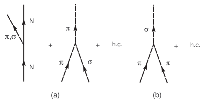
Figure 1: Decomposition of the interactions into the interactions of ”virtual” processes (a) and ”real” processes (b). The solid and broken lines stand for nucleons and mesons, respectively.

We derive the effective nuclear Hamiltonian by using the the unitary transformation described in Ref. [4]. We define the nuclear Hamiltonian as follows:

$$H_{eff} = U^{\dagger}HU.$$ (10)

Here, the unitary transformation $U=\exp(iS)\exp(iS^{\prime})$ is chosen so as to eliminate the interactions, which correspond to the ’virtual’ processes, from the Hamiltonian, while the interactions which correspond to the ’real’ processes are kept in the transformed Hamiltonian. The interactions for ’virtual processes’ of $H_{I}$ in our present model are shown in Fig. 1(a), while those for the ’real processes’($H_{\sigma\pi\pi}^{P}$), in Fig. 1(b). Then, the Hamiltonian transformed by $\exp(iS)$ newly involves the interactions which correspond to higher order ”virtual” processes. A typical term is shown in Fig. 2, which should be eliminated by the second order unitary transformation $\exp(iS^{\prime})$.

These observations fix the unitary transformation as follows:

$$H_{\pi NN}+H_{\sigma NN}+H_{\sigma\pi\pi}^{Q}+[H_{0},iS] = 0,$$ (11)

$$\frac{1}{2}[H_{I}+H_{\sigma\pi\pi}^{P},iS]^{Q}+[H_{0},iS^{\prime}]=0,$$ (12)

where the superscripts $P$ and $Q$ stand for the interactions corresponding to ’real’ and ’virtual’ processes, respectively. Then the effective Hamiltonian is given as

$$H_{eff} = U^{\dagger}HU$$ (13)

$$= H_{0}+H_{\sigma\pi\pi}^{P}+\frac{1}{2}[H_{I}+H_{\sigma\pi\pi}^{P},iS]^{P}+\frac{1}{3}[[H_{I}+\frac{1}{2}H_{\sigma\pi\pi}^{P},iS],iS]^{P}+\cdots.$$

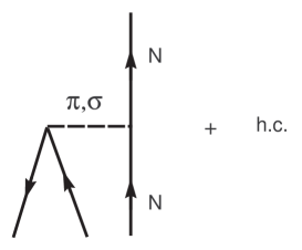
Figure 2: Interaction of ”virtual” process of order newly generated by the transformation. See the caption of Fig.1.

Here we have omitted the higher order terms in the effective Hamiltonian, since we restrict ourselves to the discussion of the effective nuclear Hamiltonian in the one-boson-exchange approximation. The lowest order effective Hamiltonian $H_{0}$ describes the free energies of mesons and nucleons. It is noticed that we do not find the operators for the pion production-absorption by a nucloen, since the interaction Hamiltonian ($H_{\pi NN}$) which produces a virtual pion by a nucleon was already eliminated from the Hamiltonian. As a result, elimination of the interaction for ’virtual process’ generates the effective many-body interactions, such as nucleon-nucleon potential, pion-nucleon potential, the interaction for pion production-absorption by two-nucleons, and so on. For the purpose of the discussion in the later sections, we shall give the explicit form of the effective interactions in the momentum space.

The third term on the righthand side of Eqn.(13) gives the one-boson-exchange nuclear potential $V_{NN}$ expressed as

$$V_{NN} = \frac{1}{2}[H_{I},iS]^{P}_{NN}$$ (14)

$$= \frac{1}{2(2\pi)^{3}}\sum_{M=\pi^{b},\sigma}D_{V}{}[\bar{u}(\mbox{\boldmath{$p$}}_{1}^{\prime})\Gamma_{M}u(\mbox{\boldmath{$p$}}_{1})]{}[\bar{u}(\mbox{\boldmath{$p$}}_{2}^{\prime})\Gamma_{M}u(\mbox{\boldmath{$p$}}_{2})],$$ (15)

where the $\Gamma_{M}$ stands for the vertex of a meson($M=\pi,\sigma$) and a nucleon ,i.e., $\Gamma_{\pi^{b}}=ig\gamma_{5}\tau^{b}$ for $\pi$ and $\Gamma_{\sigma}=g$ for $\sigma$, respectively. The function $D_{V}$ is defined as

$$D_{V} = \frac{1}{\Delta_{1}^{2}-\omega_{M}^{2}(\mbox{\boldmath{$k$}}_{1})}+\frac{1}{\Delta_{2}^{2}-\omega_{M}^{2}(\mbox{\boldmath{$k$}}_{2})}.$$ (16)

Here we introduced the energy variables as follows: $\Delta_{i}=E_{N}(\mbox{\boldmath{$p$}}_{i})-E_{N}(\mbox{\boldmath{$p$}}_{i^{\prime}})$, $\mbox{\boldmath{$k$}}_{i}=\mbox{\boldmath{$p$}}_{i}-\mbox{\boldmath{$p$}}_{i^{\prime}}$, $E_{N}(\mbox{\boldmath{$p$}})=\sqrt{M_{N}^{2}+\mbox{\boldmath{$p$}}^{2}}$ and $\omega_{M}(\mbox{\boldmath{$k$}})=\sqrt{m_{M}^{2}+\mbox{\boldmath{$k$}}^{2}}$ ($M=\pi,\sigma$). It is noticed that $\mbox{\boldmath{$p$}}_{i}$ and $\mbox{\boldmath{$p$}}_{i}^{\prime}$ are momentum operators operating initial and final nuclear wave functions, respectively.

The remaining terms in Eq. (13) give pion production operator $W$ in one-boson-exchange model,

$$W = \frac{1}{3}[[H_{I}+\frac{1}{2}H_{\sigma\pi\pi}^{P},iS],iS]^{P}_{NN}$$ (17)

$$= W_{\pi}+W_{\sigma}+W_{\pi\sigma},$$ (18)

which consists of $\pi$-exchange $W_{\pi}$, $\sigma$-exchange $W_{\sigma}$ shown in Figs 3(a) and 3(b), and $\pi-\sigma$ exchange mechanism $W_{\pi\sigma}$ shown in Fig. 3(c). The explicit form of the production operator of a pion with momentum $q$ and isospin $a$ in the momentum space is given as

$$W_{\pi}+W_{\sigma} = \frac{1}{3}\frac{1}{(2\pi)^{3}\sqrt{(2\pi)^{3}2\omega_{\pi}(\mbox{\boldmath{$q$}})}}\sum_{M=\pi^{b},\sigma}{}[\bar{u}(\mbox{\boldmath{$p$}}_{1}^{\prime})(\Gamma_{\pi^{a}}D_{W}\Gamma_{M}-\Gamma_{M}D_{W^{\prime}}\Gamma_{\pi^{a}})u(\mbox{\boldmath{$p$}}_{1})]$$ (19)

$$\times{}[\bar{u}(\mbox{\boldmath{$p$}}_{2}^{\prime})\Gamma_{M}u(\mbox{\boldmath{$p$}}_{2})]+(1\leftrightarrow 2),$$

The interaction for diagrams in Fig. 3(a) is expressed by the term with $D_{W}$, which consists of terms $D_{i+}$ and $D_{i-}$ of the intermediate nucleon states with positive and negative energy, respectively, defined by

$$D_{W} = D_{1+}+D_{1-}+D_{2+}+D_{2-},$$

$$D_{1\pm} = \Lambda^{\pm}(\mbox{\boldmath{$p$}}_{n})\frac{\Delta_{n\pm}-\Delta_{2}}{(\Delta^{2}_{n\pm}-\omega^{2}_{M}(\mbox{\boldmath{$k$}}_{2}))(\Delta^{2}_{2}-\omega^{2}_{M}(\mbox{\boldmath{$k$}}_{2}))},$$

$$D_{2\pm} = \Lambda^{\pm}(\mbox{\boldmath{$p$}}_{n})\frac{1}{\bar{\Delta}_{n\pm}+\omega_{\pi}(\mbox{\boldmath{$q$}})}(\frac{1}{\Delta^{2}_{n\pm}-\omega^{2}_{M}(\mbox{\boldmath{$k$}}_{2})}+\frac{2}{\Delta^{2}_{2}-\omega^{2}_{M}(\mbox{\boldmath{$k$}}_{2})}).$$ (20)

with $\Lambda^{+}(\mbox{\boldmath{$p$}})=u(\mbox{\boldmath{$p$}})\bar{u}(\mbox{\boldmath{$p$}})$ and $\Lambda^{-}(\mbox{\boldmath{$p$}})=v(-\mbox{\boldmath{$p$}})\bar{v}(-\mbox{\boldmath{$p$}})$. The momentum $\mbox{\boldmath{$p$}}_{n}$ ($=\mbox{\boldmath{$p$}}_{1}+\mbox{\boldmath{$k$}}_{2}=\mbox{\boldmath{$p$}}_{1}+\mbox{\boldmath{$p$}}_{2}-\mbox{\boldmath{$p$}}_{2}^{\prime}$) denotes the the nucleon momentum in the intermediate state. The energy variables are defined as $\Delta_{n\pm}=E_{N}(\mbox{\boldmath{$p$}}_{1})\mp E_{N}(\mbox{\boldmath{$p$}}_{n})$, and $\bar{\Delta}_{n\pm}=E_{N}(\mbox{\boldmath{$p$}}_{1}^{\prime})\mp E_{N}(\mbox{\boldmath{$p$}}_{n})$.

The interaction for the diagram in Fig. 3(b) is expressed by the term with $D_{W^{\prime}}$,

$$D_{W}^{\prime} = D_{1+}^{\prime}+D_{1-}^{\prime}+D_{2+}^{\prime}+D_{2-}^{\prime},$$ (21)

where the functions $D_{i\pm}^{\prime}$ are obtained from $D_{i\pm}$ by replacing $\mbox{\boldmath{$p$}}_{n}$, $\Delta_{n\pm}$ and $\Delta_{n^{\prime}\pm}$ by $\mbox{\boldmath{$p$}}_{n}^{\prime}=\mbox{\boldmath{$p$}}_{1}^{\prime}-\mbox{\boldmath{$k$}}_{2}$, $\Delta_{n^{\prime}\pm}=-E_{N}(\mbox{\boldmath{$p$}}_{1}^{\prime})\pm E_{N}(\mbox{\boldmath{$p$}}_{n}^{\prime})$ and $\bar{\Delta}_{n^{\prime}\pm}=-E_{N}(\mbox{\boldmath{$p$}}_{1})\pm E_{N}(\mbox{\boldmath{$p$}}_{n}^{\prime})$, respectively.

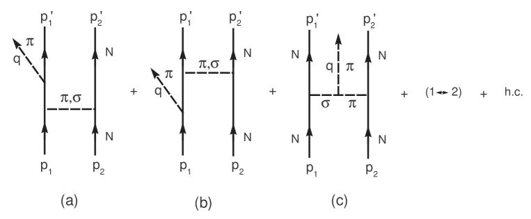
Figure 3: Pion Production by two nucleons. Figs.(a) and (b) show the nucleon-pole diagrams, while fig.(c) shows the sigma-pion exchange diagram.

Structure of the $D_{1\pm}$ terms is the same as the one of the corresponding diagrams in the meson-exchange current[4, 8]. For the discussion in later section, let us investigate the matrix element $D$ at the threshold of pion production ($\mbox{\boldmath{$q$}}=0$) in the center of mass system ($\mbox{\boldmath{$p$}}_{1}=-\mbox{\boldmath{$p$}}_{2}$ and $\mbox{\boldmath{$p$}}_{1}^{\prime}=-\mbox{\boldmath{$p_{2}^{\prime}$}}$). We notice that $\Delta_{n+}=\Delta_{2}$ and $D_{1+}$ vanishes. This is well known as a fact that the recoil and renormalization currents cancel each other for the vanishing momentum $q$ in the meson-exchange current. On the other hand the $D_{2+}$ term remains finite, and can be expressed in terms of the commutator of the ”conventional” single-nucleon pion production operator and the nuclear potential. The pion production operator $(W_{\pi}+W_{\sigma})_{+}$ with the intermediate nucleon state of positive energy at threshold is simply expressed as

$$(W_{\pi}+W_{\sigma})_{+} = \frac{1}{m_{\pi}}[H_{\pi NN},V_{NN}].$$ (22)

Note that the $D_{1-}$ and $D_{2-}$ terms as well as the $W_{\pi\sigma}$ term remain to be finite. Details of the latter term are separately discussed in Appendix.

As a result, our effective nuclear Hamiltonian in one-boson-exchange approximation is expressed as follows:

$$H_{eff}=H_{0}+H_{\sigma\pi\pi}^{P}+V_{\pi N}+V_{NN}+W.$$ (23)

It is noticed that we have still the pion degree of freedom as expressed by the terms $V_{\pi N},W,H^{P}_{\sigma\pi\pi}$ in our effective Hamiltonian. The nuclear state vector is determined by solving the coupled channel equations of the above effective Hamiltonian in the $NN$ and $\pi NN$ Fock space.

3 Effective Nuclear Axial-Vector Current

We shall derive the nuclear axial-vector current, by transforming the axial-vector current (8) and (9) under the same unitary transformation $U$ as used in deriving the effective nuclear Hamiltonian. This is important to make the theory self-consistent.

$$A_{eff}^{\mu a}(x) = U^{\dagger}A^{\mu a}(x)U,$$ (25)

$$= A^{\mu a}+[A^{\mu a},iS]+\frac{1}{2}[[A^{\mu a}+\frac{1}{3}[A^{\mu a},iS],iS],iS]$$

$$+[A^{\mu a}+[A^{\mu a},iS],iS^{\prime}].$$

The effective nuclear current consists of meson current($A^{\mu a}_{M}$), the nucleon current ($A^{\mu a}_{N}$) and meson exchange current ($A^{\mu a}_{NN}$). Existence of the meson current with the same form as the original one is essentially important to describe axial-vector current in the $\pi NN$ Fock space. The nucleon current including pion pole term in the momentum space is given as

$$A_{N}^{\mu a} = \bar{u}(\mbox{\boldmath{$p$}}^{\prime})a^{\mu a}_{N}(p^{\prime},p)u(\mbox{\boldmath{$p$}}),$$ (26)

with

$$a_{N}^{\mu a}(p^{\prime},p) = [\gamma^{\mu}\gamma_{5}-\frac{2gf_{\pi}(p^{\prime}-p)^{\mu}}{(p^{\prime}-p)^{2}-m_{\pi}^{2}}\gamma_{5}]\frac{\tau^{a}}{2}.$$ (27)

Here four vector $p(p^{\prime})$ is defined as $p^{\mu}=(E_{N}(\mbox{\boldmath{$p$}}),\mbox{\boldmath{$p$}})$.

The meson exchange current consists of pion-exchange current $(A^{\mu a}_{NN\pi})$, sigma-exchange current $(A^{\mu a}_{NN\sigma})$ and pi-sigma-exchange current $(A^{\mu a}_{NN\pi\sigma})$. The explicit form of the exchange current is given by

$$A^{\mu a}_{NN\pi}+A^{\mu a}_{NN\sigma} = \frac{1}{2(2\pi)^{3}}\sum_{M=\pi^{b},\sigma}{}[\bar{u}(\mbox{\boldmath{$p$}}_{1}^{\prime})(a^{\mu a}_{NN}\Gamma_{M}-\Gamma_{M}a^{\mu a}_{NN^{\prime}})u(\mbox{\boldmath{$p$}}_{1})]$$ (28)

$$\times[\bar{u}(\mbox{\boldmath{$p$}}_{2}^{\prime})\Gamma_{M}u(\mbox{\boldmath{$p$}}_{1})]+(1\leftrightarrow 2),$$

with

$$a^{\mu a}_{NN} = \bar{a}^{\mu a}_{N}(p_{1}^{\prime},p_{n+})D_{1+}+\bar{a}^{\mu a}_{N}(p_{1}^{\prime},p_{n-})D_{1-}+a^{\mu a}_{N}(p_{1}^{\prime},p_{n-})D_{3-},$$ (29)

$$a^{\mu a}_{NN^{\prime}} = D_{1+}^{\prime}\bar{a}^{\mu a}_{N}(p_{n^{\prime}+},p_{1})+D_{1-}^{\prime}\bar{a}^{\mu a}_{N}(p_{n^{\prime}-},p_{1})+D_{3-}^{\prime}a^{\mu a}_{N}(p_{n^{\prime}-},p_{1}),$$ (30)

and

$$\bar{a}_{N}^{\mu a}(p^{\prime},p) = [\gamma^{\mu}\gamma_{5}-\frac{1}{3}\frac{2gf_{\pi}}{(p^{\prime}-p)^{2}-m_{\pi}^{2}}(p^{\prime}-p)^{\mu}\gamma_{5}]\frac{\tau^{a}}{2},$$ (31)

$$D_{3-} = \Lambda^{-}(\mbox{\boldmath{$p$}}_{n})\frac{1}{\Delta_{n-}+\Delta_{2}}{}[\frac{1}{\Delta^{2}_{n-}-\omega^{2}_{M}(\mbox{\boldmath{$k$}}_{2})}+\frac{1}{\Delta^{2}_{2}-\omega^{2}_{M}(\mbox{\boldmath{$k$}}_{2})}].$$ (32)

Here four-vectors are defined as ${p^{\prime}_{1}}^{\mu}=(E_{N}(\mbox{\boldmath{$p$}}_{1}^{\prime}),\mbox{\boldmath{$p$}}_{1}^{\prime})$, $p^{\mu}_{n\pm}=(\pm E_{N}(\mbox{\boldmath{$p$}}_{n}),\mbox{\boldmath{$p$}}_{n})$ and $p^{\mu}_{n^{\prime}\pm}=(\pm E_{N}(\mbox{\boldmath{$p$}}_{n}^{\prime}),\mbox{\boldmath{$p$}}_{n}^{\prime})$. It is noticed that the energy variable $E_{N}(\mbox{\boldmath{$p$}})$ is a function of the momentum operator $p$. The $D_{1\pm}$ term, which appeared in the pion production operator, is exactly the same as a sum of the recoil, renormalization and pair currents.

Although we have no terms with $D_{2\pm}$, which is related to nuclear potential, in the meson-exchange current, we have a new pair-current $D_{3-}$ expressed as a commutator of the nucleon-current and the operator $S^{\prime}$ of the unitary transformation associated with the interaction shown in Fig.2. The term $D_{3-}^{\prime}$ is obtained from $D_{3-}$ by replacing the momenta in the same way as was done for obtaining $D^{\prime}_{i\pm}$ in the previous section.

We also have the meson-exchange current with $\pi\sigma$ exchange mechanism, which is summarized in Appendix, and is discussed with the corresponding operator of the pion production.

Consequently, the total effective nuclear axial-vector current consists of the one-nucleon current (the impulse current ) $A_{N}^{\mu a}$, meson current $A_{M}^{\mu a}$ and the meson-exchange current $A_{NN}^{\mu a}$:

$$A_{eff}^{\mu a}(\mbox{\boldmath{$x$}})=A_{N}^{\mu a}(\mbox{\boldmath{$x$}})+A_{M}^{\mu a}(\mbox{\boldmath{$x$}})+A_{NN}^{\mu a}(\mbox{\boldmath{$x$}}).$$ (33)

4 Nuclear Axial-Vector Current and PCAC Relation

The basic Hamiltonian and axial-vector current of the $\sigma$-model satisfies the PCAC relation.

$$\mbox{\boldmath{$\nabla$}}\cdot\mbox{\boldmath{$A$}}^{a}+i[H,A^{0a}]=-f_{\pi}m_{\pi}^{2}\pi^{a}.$$ (34)

In the present treatment, the PCAC relation is transformed as

$$\mbox{\boldmath{$\nabla$}}\cdot\mbox{\boldmath{$A$}}_{eff}^{a}\ +\ i[\ H_{eff}\ ,A_{eff}^{0a}\ ]=-f_{\pi}m_{\pi}^{2}\Pi_{eff}^{a}.$$ (35)

The effective pion field $\Pi_{eff}^{a}$ is given by the unitary transformation of the pion field as

$$\Pi_{eff}^{a} = U^{\dagger}\pi^{a}U,$$ (36)

and can be given in one-boson-exchange approximation as

$$\Pi_{eff}^{a} = \pi^{a}+\Pi^{a}_{N}+\Pi^{a}_{NN}.$$ (37)

It is easily shown that the effective axial-vector current, the effective nuclear Hamiltonian, and the effective pion field satisfy the PCAC relation: The relation can be divided into three parts,1) meson current, 2) one-nucleon current and 3) exchange current:

1) The meson current
The meson current ($\mbox{\boldmath{$A$}}_{M}^{a},A_{M}^{0a}$) satisfies

$$\mbox{\boldmath{$\nabla$}}\cdot\mbox{\boldmath{$A$}}_{M}^{a}+i[H_{0},A_{M}^{0a}]=-f_{\pi}m_{\pi}^{2}\pi^{a}.$$ (38)

It is noticed this is a consequence of existence of the meson degrees of freedom in our nuclear Hamiltonian. Without these freedoms, one cannot satisfy the PCAC relation.
2) The one-nucleon current
The one-body current satisfies the relation very familiar to us:

$$\mbox{\boldmath{$\nabla$}}\cdot\mbox{\boldmath{$A$}}_{N}^{a}+i[H_{0},A_{N}^{0a}]=-f_{\pi}m_{\pi}^{2}\Pi_{N}^{a},$$ (39)

with

$$\Pi_{N}^{a} = \frac{1}{(p^{\prime}-p)^{2}-m_{\pi}^{2}}\bar{u}(\mbox{\boldmath{$p$}}^{\prime})\Gamma_{\pi^{a}}u(\mbox{\boldmath{$p$}}),$$ (40)

3) The meson-exchange current
The PCAC relation for the meson-exchange current is non-trivial. It is expressed as follows:

$$\mbox{\boldmath{$\nabla$}}\cdot\mbox{\boldmath{$A$}}_{NN}^{a}+i\Bigl{[}H_{0},A_{NN}^{0a}\Bigr{]}+i\Bigl{[}V_{NN},A_{N}^{0a}\Bigr{]}+i\Bigl{[}W_{\pi},A_{M}^{0a}\Bigr{]}$$

$$=-f_{\pi}m_{\pi}^{2}\Pi_{NN}^{a}.$$ (41)

Here it is noticed that the above equation includes the meson-exchange current, the one-nucleon current and also meson-current. Thus, in order to complete the PCAC relation, we need the meson current and the pion production-absorption operator in addition to the nuclear potential and meson-exchange current. This fact has been overlooked in the previous works so far done.

5 Relation of Pion Production and the PCAC

We shall investigate the relation of pion production reaction and the PCAC relation. In order to avoid unnecessary complications, we shall assume the nuclear system with two nucleons and pions. The relation of the one-body axial-vector current in Eqs. (4.6) and (4.7) suggests that one can obtain pion production operator by using the PCAC relation. However the PCAC relation connects divergence of the axial-vector current with the the effective pion field operator, but not the pion production operator to be used in the dynamical equations describing the nuclear system with nucleons and pions. By using the reduction formula, we have a relation between the matrix element of the divergence of the axial-vector current and the pion production T-matrix element as

$$iq^{\mu}\langle NN|A_{\mu}^{a}|NN\rangle = \frac{f_{\pi}m_{\pi}^{2}}{q^{2}-m_{\pi}^{2}}\sqrt{(2\pi)^{3}2\omega_{\pi}(k)}T_{NN\rightarrow\pi NN}$$ (42)

with the pion momentum $q^{\mu}$, which should hold for any formalism to describe nuclear system. It is noticed that the $NN\rightarrow\pi NN$ T-matrix is calculated by solving the coupled channel equations for the nuclear system. At first sight, one may point out that this equality contradicts with our present theory, because the left-hand side of the equation includes the matrix elements of the one-nucleon operator, while the right-hand side of the equation does not. Absence of the one-nucleon operator for the pion production, however, does not lead to any contradiction, since the pion in the final state is always produced from a nucleon interacting with other nucleons. In other words, this observation shows that we evaluate the matrix element of the two-nucleon operator such as a product of the one-boson-exchange potential and the one-nucleon pion production operator, which corresponds to our pion production operator $(W_{\sigma}+W_{\pi})$ .

To show that this is really the case, we shall investigate the matrix element of the pion production operator $(W_{\sigma}+W_{\pi})_{+}$ at threshold. (Since other terms in $(W_{\sigma}+W_{\pi})$ are essentially irrelevant to the two-nucleon potential, we shall safely skip them from the discussion in what follows.) Now we calculate the T-matrix element by using the solution of the coupled channel equation in the lowest order:

$$T_{NN\rightarrow\pi NN} \sim <NN_{f}(DW)|(W_{\pi}+W_{\sigma})_{+}|NN_{i}(DW)>.$$ (43)

Here the $|NN_{i/f}(DW)>$ are the nuclear state vectors with energy $E_{i/f}$ obtained by solving Schrödinger equation. Using Eq. (22) and noticing $[H_{0},H_{\pi NN}]=0$ at threshold($E_{i}-E_{f}=m_{\pi}$), we can rewrite Eq. (43) as

$$T_{NN\rightarrow\pi NN} = <NN_{f}(DW)|\frac{1}{m_{\pi}}[H_{\pi NN},H_{0}+V_{NN}]|NN_{i}(DW)>$$ (44)

$$= <NN_{f}(DW)|H_{\pi NN}|NN_{i}(DW)>.$$ (45)

This is just the matrix element of the pion source function of the one-nucleon type. Therefore, our pion-production operator is consistent with the PCAC relation.

The present result also implies that the PCAC relation requires us to construct the nuclear force, pion production operator and exchange currents in a consistent way, and also to describe the nuclear system including the pion degree of freedom based on the nuclear force thus derived.

6 Summary

We have studied the nuclear PCAC relation in the recent theory of the effective nuclear interactions which include meson degrees of freedom explicitly. First of all, in order to make the discussion clear, we assumed the linear $\sigma$-model, and derived the nuclear force, the effective interaction for the pion production-absorption and the nuclear axial-vector current by applying the unitary transformation. All the operators we have derived are Hermitian and are functions of the local momenta of the relevant particles. Secondly, we have studied in detail the nuclear PCAC relation , in particular, relationship among the pion-production mechanism, the axial-vector current and the nuclear force. As results, 1) it was shown that one has to take into account the explicit pion and sigma meson degrees of freedom in addition to the nucleons in order to satisfy the PCAC relations. In particular, a consistent description of the nculear force, and also pion production operator played an essential role to hold the PCAC relation. 2) The PCAC relation gives us just the effective pion field, but not the interactions for the pion production-absorption processes. 3) The fact that the one-body pion production operator does not exist in our formalism means simply that a free nucleon cannot emit or absorb a pion. As a consequence, the effective interaction operator for pion production-absorption includes the term which corresponds to production of a pion by a nucleon interacting with other nucleons, in addition to the conventional irreducible two-nucleon operators. This looks similar to the traditional approach which incorporate the one-nucleon operator plus nuclear correlations, as far as we concern ourselves with the pion production at threshold.

It is noticed that the above observations about the nuclear PCAC relation holds independent of any strong interaction models which lead the PCAC relation. Equations (4.8) and (5.1) showed that the PCAC relation for the two-nucleon axial-vector current is not a simple relation assumed by Blin-Stoyle and Tint for the Gamow-Teller operator.

To make the nuclear axial-vector current and pion production-absorption operators more realistic, we should incorporate short-range mechanism into the present work starting, for example from the model based on chiral symmetry[9, 10].

Appendix A $\sigma\pi$ exchange current and pion production operator

Here we give full expressions for the $\sigma-\pi$ exchange current and pion production operator. The pion production operator is given as

$$W_{\pi\sigma} = \frac{m_{\sigma}^{2}-m_{\pi}^{2}}{f_{\pi}(2\pi)^{3}\sqrt{(2\pi)^{3}2\omega_{\pi}(\mbox{\boldmath{$q$}})}}{}[\bar{u}(\mbox{\boldmath{$p$}}_{1}^{\prime})\Gamma_{\sigma}u(\mbox{\boldmath{$p$}}_{1})]{}[\bar{u}(\mbox{\boldmath{$p$}}_{2}^{\prime})\Gamma_{\pi^{a}}u(\mbox{\boldmath{$p$}}_{2})]D_{\pi\sigma}+(1\leftrightarrow 2),$$

where

$$D_{\pi\sigma} = D_{M}[1+\frac{\Delta_{1}+\Delta_{2}-\omega_{\pi}(\mbox{\boldmath{$q$}})}{12\omega_{\sigma}\omega_{\pi}}(\frac{(\Delta_{1}-\omega_{\sigma})(\Delta_{2}-\omega_{\pi})}{\omega_{\sigma}+\omega_{\pi}+\omega_{\pi}(\mbox{\boldmath{$q$}})}$$ (47)

$$-\frac{(\Delta_{1}+\omega_{\sigma})(\Delta_{2}+\omega_{\pi})}{\omega_{\sigma}+\omega_{\pi}-\omega_{\pi}(\mbox{\boldmath{$q$}})}-\frac{(\Delta_{1}-\omega_{\sigma})(\Delta_{2}+\omega_{\pi})}{\omega_{\sigma}-\omega_{\pi}+\omega_{\pi}(\mbox{\boldmath{$q$}})})]$$

with

$$D_{M} = \frac{1}{(\Delta_{1}^{2}-\omega_{\sigma}^{2})(\Delta_{2}^{2}-\omega_{\pi}^{2})}$$ (48)

Here we denote $\omega_{\sigma}=\omega_{\sigma}(\mbox{\boldmath{$k$}}_{1})$ and $\omega_{\pi}=\omega_{\pi}(\mbox{\boldmath{$k$}}_{2})$. The second term in the square bracket proportional to $\Delta_{1}+\Delta_{2}-\omega_{\pi}(\mbox{\boldmath{$q$}})$ vanishes in the Born approximation because of the energy conservation, and it contributes to the off -energy shell matrix element.

The axial-vector exchange current is given as

$$A_{NN\pi\sigma}^{\mu a} = \frac{1}{(2\pi)^{3}}D_{M}^{\mu}{}[\bar{u}(\mbox{\boldmath{$p$}}_{1}^{\prime})\Gamma_{\sigma}u(\mbox{\boldmath{$p$}}_{1})]{}[\bar{u}(\mbox{\boldmath{$p$}}_{2}^{\prime})\Gamma_{\pi^{a}}u(\mbox{\boldmath{$p$}}_{2})]+(1\leftrightarrow 2).$$ (49)

The non pion-pole term of the exchange current is simply given as

$$D_{M}^{\mu} = i(p_{1}-p_{1}^{\prime}-p_{2}+p_{2}^{\prime})^{\mu}D_{M},$$ (50)

while the pion-pole term is given as

$$\mbox{\boldmath{$D$}}_{M} = -i(\mbox{\boldmath{$p$}}_{1}+\mbox{\boldmath{$p$}}_{2}-\mbox{\boldmath{$p$}}_{1}^{\prime}-\mbox{\boldmath{$p$}}_{2}^{\prime})$$ (51)

$$\times\frac{m_{\sigma}^{2}-m_{\pi}^{2}}{6\omega_{\sigma}\omega_{\pi}}(\frac{\Delta_{1}\Delta_{2}+\omega_{\sigma}\omega_{\pi}}{(\omega_{\sigma}+\omega_{\pi})^{2}-\omega_{\pi}(\mbox{\boldmath{$q$}})}+\frac{\Delta_{1}\Delta_{2}-\omega_{\sigma}\omega_{\pi}}{2\omega_{\pi}(\mbox{\boldmath{$q$}})(\omega_{\sigma}-\omega_{\pi}+\omega_{\pi}(\mbox{\boldmath{$q$}}))})D_{M},$$

$$D^{0}_{M} = -i\frac{m_{\sigma}^{2}-m_{\pi}^{2}}{6\omega_{\sigma}\omega_{\pi}}(\frac{(\omega_{\sigma}+\omega_{\pi})(\Delta_{1}\omega_{\pi}+\Delta_{2}\omega_{\sigma})}{(\omega_{\sigma}+\omega_{\pi})^{2}-\omega_{\pi}(\mbox{\boldmath{$q$}})^{2}}-\frac{\Delta_{2}\omega_{\sigma}-\Delta_{1}\omega_{\pi}}{2(\omega_{\sigma}-\omega_{\pi}+\omega_{\pi}(\mbox{\boldmath{$q$}}))})D_{M}.$$

References

- [1] I. Towner, \PRP155,1987,263
- [2] R.J. Blin-Stoyle and M. Tint, Phys. Rev. 160 (1967), 803
- [3] J.Bernabu, T.E.O.Ericson and C.Jarlskog, \PLB69,1977,161
- [4] M. Kobayashi, T. Sato and H. Ohtsubo, \PTP98,1997,927
- [5] A. V. Shebeko and M. I. Shirokov, Prog. Part. Nucl. Phys. 44 (2000), 75
- [6] V. Dmitrainovi and T. Sato, \PRC58,1998,1937
- [7] M. Gell-Mann and M. Lvy, \NC16,1960,53
- [8] Y. Futami, J. -I. Fujita and H. Ohtsubo, \PTPS60,1976,83
- [9] J. Adam Jr., Ch. Hajduk, H. Henning, P. U. Sauer and E. Truhlik, \NPA531,1991,623
- [10] S. M. Ananyan, B. D. Serot, J. D. Walecka, \PRC66,2002,055502