Nuclear $(\mu^{-},e^{+})$ conversion mediated by Majorana neutrinos

Abstract

We study lepton number violating (LNV) process of $(\mu^{-},e^{+})$ conversion in nuclei mediated by the exchange of light and heavy Majorana neutrinos. Nuclear structure calculations have been carried out for the case of experimentally interesting nucleus ${{}^{48}\mathrm{Ti}}$ in the framework of renormalized proton-neutron Quasiparticle Random Phase Approximation. We demonstrate that the imaginary part of the amplitude of light Majorana neutrino exchange mechanism gives an appreciable contribution to the $(\mu^{-},e^{+})\$conversion rate. This specific feature is absent in the allied case of $0\nu\beta\beta$ decay. Using the present neutrino oscillations, tritium beta decay, accelerator and cosmological data we derived the limits on the effective masses of light ${\langle m\rangle_{\mu e}}$ and heavy $\langle M_{N}^{-1}\rangle_{\mu e}$ neutrinos. The expected rates of nuclear $(\mu^{-},e^{+})\$conversion, corresponding to these limits, were found to be so small that even within a distant future the $(\mu^{-},e^{+})\$conversion experiments will hardly be able to detect the neutrino signal. Therefore, searches for this LNV process can only rely on the presence of certain physics beyond the trivial extension of the Standard Model by inclusion of massive Majorana neutrinos.

I Introduction

Lepton number ($L$) conservation is one of the most obscure sides of the Standard Model (SM) not supported by an underlying principle and following from an accidental interplay between gauge symmetry and field content. Any deviation from the SM structure may introduce $L$ non-conservation (LNV). Over the years the possibility of lepton number non-conservation has been attracting a great deal of theoretical and experimental efforts since any positive experimental signal of LNV would point to physics beyond the SM. The simplest extension of the SM allowing LNV processes implies inclusion of massive Majorana neutrinos with the $\Delta L=2$ mass term introducing the necessary source of LNV. However, the role of neutrinos in LNV processes is more intricate. The fundamental fact Schechter and Valle (1982) consists in the following: observation of any LNV process would prove that neutrinos are massive Majorana particles. This is true even if their direct contribution to this process is negligible and the dominant contribution has nothing to do with neutrinos.

Recent neutrino oscillation experiments established the presence of small non-zero neutrino masses, the fact that itself points to physics beyond the SM. However neutrino oscillations are not sensitive to the nature of neutrinos: they could be either Majorana or Dirac particles leading to the same oscillation observables.

The principal question if neutrinos are Majorana or Dirac particles can be answered only by searching for LNV processes which, as commented above, are intimately related to the nature of neutrinos.

Various LNV processes have been discussed in the literature in this respect (for review see Dib et al. (2001)). In principle, they can probe Majorana neutrino contribution and provide information on the so called effective masses $\langle m_{\nu}\rangle_{\alpha\beta}$ and $\langle M_{N}^{-1}\rangle_{\alpha\beta}$ of light and heavy Majorana neutrinos (for definition see Sect. II). These quantities under certain assumptions are related to the entries of the Majorana neutrino mass matrix $M_{\alpha\beta}^{(\nu)}$.

Among these processes there are a few LNV nuclear processes having prospects for experimental searches: neutrinoless double beta decay ($0\nu\beta\beta$), muon to positron $(\mu^{-},e^{+})$ conversion and, probably, muon to antimuon $(\mu^{-},\mu^{+})$ conversion Missimer et al. (1994); Simkovic et al. (2002a).

Currently the most sensitive experiments intended to distinguish the Majorana nature of neutrinos are those searching for $0\nu\beta\beta$-decay  Klapdor-Kleingrothaus et al. (2001); Aalseth et al. (2002); Arnaboldi et al. (2004); Elliott and Vogel (2002). The nuclear theory side Doi et al. (1985); Faessler and Šimkovic (1998); Suhonen and Civitarese (1998) of this process has been significantly improved in the last decade (see also Elliott and Engel (2004); Rodin et al. (2003); Bilenky et al. (2004) and references therein) allowing reliable extraction of fundamental particle physics parameters from experimental data.

The $(\mu^{-},e^{+})$ conversion is another LNV nuclear process searched for experimentally. The important role of muon as a test particle for new physics beyond the SM has been recognized long time ago. When negative muons penetrate into matter they can be trapped to atomic orbits. Then the bound muon may disappear either decaying into one electron and two neutrinos or being captured by the nucleus, i.e., due to ordinary muon capture. These two processes, conserving both total lepton number and lepton flavors, are the SM processes and have been well studied both theoretically and experimentally. The physics beyond the SM resides in yet non-observed channels of muon capture: muon-electron ($\mu^{-},e^{-}$) and muon-positron ($\mu^{-},e^{+}$) conversions in nuclei Kamal and Ng (1979); Vergados (1981); Vergados and Ericson (1982); Leontaris and Vergados (1983); Kosmas et al. (1994, 1997); Faessler et al. (2000); Šimkovic et al. (2001); Divari et al. (2001, 2002); Kosmas et al. (2001a, b); Simkovic et al. (2002b); Kosmas (2002); Kosmas et al. (2003); Faessler et al. (2004):

$$\begin{split}(A,Z)+\mu_{\mathrm{b}}^{-}&\rightarrow e^{-}+(A,Z)^{*},\\ (A,Z)+\mu_{\mathrm{b}}^{-}&\rightarrow e^{+}+(A,Z-2)^{*}.\end{split}$$ (1)

Apparently, the ($\mu^{-},e^{-}$) conversion process violate lepton flavor $L_{f}$ and conserve the total lepton number $L$, while ($\mu^{-},e^{+}$) conversions violate both of them. Additional differences between the $(\mu^{-},e^{-})$ and $(\mu^{-},e^{+})$ lie on the nuclear physics side. The first process can proceed on one nucleon of the participating nucleus while the second process involves two nucleons as dictated by charge conservation Vergados (1981); Leontaris and Vergados (1983). Note also that the $(\mu^{-},e^{-})$ conversion amplitude is quadratic and $(\mu^{-},e^{+})$ amplitude linear in the light neutrino mass. Thus the second process looks more sensitive to the light neutrino masses.

The currently best experimental limit on $(\mu^{-},e^{+})$ conversion branching ratio has been established at PSI  Dohmen et al. (1993) for the ⁴⁸Ti nuclear target

$$R^{(\mu e^{+})}(Ti)=\frac{\Gamma(\mu^{-}+{{}^{48}\mathrm{Ti}}\rightarrow e^{+}+{{}^{48}\mathrm{Ca}})}{\Gamma(\mu^{-}+{{}^{48}\mathrm{Ti}}\rightarrow\nu_{\mu}+{{}^{48}\mathrm{Sc}})}<4.3\times 10^{-12}.$$ (2)

Now it is expected a significant improvement of this limit in the near future experiments: SINDRUM II (PSI) with ⁴⁸Ti target  Dohmen et al. (1993), MECO (Brookhaven) with ²⁷Al target Molzon (2002) and PRIME (Tokyo) with ⁴⁸Ti target  Kuno (2001).

In the present paper we study light and heavy Majorana neutrino exchange mechanisms of the $(\mu^{-},e^{+})$ conversion which are conceptually most natural and simple. One of the main motivations of this study comes from the nuclear physics side of this process: the nuclear theory of $(\mu^{-},e^{+})$ conversion is not yet well elaborated and may show new interesting features absent in the other LNV processes such as the $0\nu\beta\beta$-decay. For instance, as we will demonstrate, the imaginary part of the $(\mu^{-},e^{+})$ conversion amplitude in the case of light Majorana exchange gives an appreciable contribution to the rate of this process, the fact which has not been recognized for a long time. Studying the most simple case of $(\mu^{-},e^{+})$ conversion via Majorana neutrino exchange, we have in mind that this process may receive contribution from other mechanisms offered by various models beyond the SM such as the R-parity violating supersymmetric models, the leptoquark extensions of the SM etc. Some of these mechanisms may involve light or heavy neutrino exchange and, therefore, in the part of nuclear structure calculations they may resemble the ordinary neutrino mechanisms. Thus our present study can be viewed as a step towards a more general description of $(\mu^{-},e^{+})$ conversion including all the possible mechanisms.

Below, we develop a detailed nuclear structure theory for the light and heavy neutrino exchange mechanisms of this process on the basis of the nuclear proton-neutron renormalized Quasiparticle Random Phase Approximation (pn-QRPA)  Toivanen and Suhonen (1995); Schwieger et al. (1996). We calculate the nuclear matrix elements of $(\mu^{-},e^{+})$ conversion in ⁴⁸Ti, which serves as target nucleus in SINDRUM Dohmen et al. (1993) and PRIME Kuno (2001) experiments.

Existing limits on neutrino masses and mixing from neutrino oscillation phenomenology and other observational data allow us to estimate typical rate of this process, assuming the dominance of light or heavy Majorana neutrino exchange mechanisms. Extremely low values for these rates, derived in this way, leave no chance to detect a neutrino signal in the $(\mu^{-},e^{+})\$conversion even within a distant future and, thus, to derive information on the effective masses $\langle m_{\nu}\rangle_{\mu e}$ and $\langle M_{N}^{-1}\rangle_{\mu e}$ from this process. This conclusion, nevertheless, does not diminish the importance of experiments searching for $(\mu^{-},e^{+})\$conversion since its observation would be unambiguous signal of a non-trivial physics beyond the SM.

The paper is organized as follows. In Sect. II we discuss some general issues of Majorana neutrinos for LNV processes. Sect. III deals with the current limits on the effective Majorana neutrino masses entering to the $(\mu^{-},e^{+})$ conversion amplitude. The amplitude and rate of $(\mu^{-},e^{+})$ conversion are derived in Sect. IV. The details of nuclear calculations for $(\mu^{-},e^{+})$ conversion in ⁴⁸Ti are given in Sect. V. In Sect. VI we discuss the possible impact of $(\mu^{-},e^{+})\$conversion experiments on neutrino physics and visa versa. In Sect. VII we summarize our results and conclusions.

II Majorana neutrinos in LNV processes

The finite masses of neutrinos are tightly related to the problem of lepton flavor/number violation. The Dirac, Majorana and Dirac-Majorana neutrino mass terms in the Lagrangian offer different neutrino mixing schemes and allow various lepton number/flavor violating processes Bilenky and Petcov (1987); Bilenky et al. (1999); Zuber (2002).

Let us consider the generic case of neutrino field contents with the three left-handed weak doublet neutrinos $\nu^{\prime}_{Li}=(\nu^{\prime}_{Le},\nu^{\prime}_{L\mu},\nu^{\prime}_{L\tau})$ and $n$ species of the SM singlet right-handed neutrinos $\nu^{\prime}_{Ri}=(\nu^{\prime}_{R1},...\nu^{\prime}_{Rn})$. The mass term for this set of fields can be written in a general form as

$$- \frac{1}{2}\overline{\nu^{\prime}}{\cal M}^{(\nu)}\nu^{\prime c}+\mbox{H.c.}=-\frac{1}{2}(\bar{\nu}^{\prime}_{{}_{L}},\overline{\nu_{{}_{R}}^{\prime c}})\left(\begin{array}[]{cc}{\cal M}_{L}&{\cal M}_{D}\\ {\cal M}^{T}_{D}&{\cal M}_{R}\end{array}\right)\left(\begin{array}[]{c}\nu_{{}_{L}}^{\prime c}\\ \nu^{\prime}_{{}_{R}}\end{array}\right)+\mbox{H.c.}=$$ (7)

$$- \frac{1}{2}\sum_{i=1}^{3+n}m_{i}\overline{\nu^{c}}_{i}\nu_{i}+\mbox{H.c.}$$ (8)

Here ${\cal M}_{L},{\cal M}_{R}$ are $3\times 3$ and $n\times n$ symmetric Majorana mass matrices, ${M}_{D}$ is $3\times n$ Dirac type matrix. Rotating the neutrino mass matrix by the unitary transformation to the diagonal form

$$U^{T}{\cal M}^{(\nu)}U=Diag\{m_{i}\}$$ (9)

we end up with $n+3$ Majorana neutrinos $\nu_{i}=U^{*}_{ki}\nu^{\prime}_{k}$ with the masses $m_{i}$. In special cases there may appear among them pairs with masses degenerate in absolute values. Each of these pairs can be collected into a Dirac neutrino field. This situation corresponds to conservation of certain lepton numbers assigned to these Dirac fields.

The considered generic model must contain at least three observable light neutrinos while the other states may be of arbitrary mass. In particular, they may include intermediate and heavy mass states. Presence or absence of these neutrino states is a question for experimental searches.

The favored neutrino model has to accommodate modern neutrino phenomenology in a natural way, in particular, to answer the question of the smallness of neutrino masses compared to the charged lepton ones. The most prominent guiding principle in this problem is the see-saw mechanism. It suggests that the typical scale of $M^{D}$ matrix elements in Eq. (7) is comparable with the masses of charged leptons meanwhile the ${\cal M}_{R}$ is associated to a large hypothetical scale of lepton number violation like $M_{LNV}\approx 10^{12}~{}\mathrm{GeV}$. Then the diagonalization in Eq. (9) brings very light $\nu_{k}$ and very heavy $N_{k}$ Majorana neutrinos. This mechanism can be realized in various models beyond the SM with significantly lower scales, $M_{LNV}\sim 1$ TeV, leading to the neutrino masses and mixing consistent with the observational data. A particular example is given by the class of supersymmetric model with bilinear R-parity violation (see, for instance, Ref. Hirsch et al. (2003) and references therein). In these models the heavy Majorana neutrinos have moderately large masses $\sim 1$TeV and even lower giving them phenomenological significance via a priori non-negligible contributions to LNV processes. In the present paper we examine the contributions of light and heavy Majorana neutrinos to $(\mu^{-},e^{+})$ conversion.

In general, the flavor neutrino states are the superpositions of light ($\nu_{k}$) and heavy ($N_{k}$) Majorana mass eigenstates:

$$\nu_{l}(x)=\sum_{k=\mathrm{light}}U_{lk}\nu_{k}(x)+\sum_{k=\mathrm{heavy}}U_{lk}N_{k}(x),$$ (10)

with the masses $m_{k}$ and $M_{k}$ respectively. Here $U$ is neutrino mixing matrix.

Now let us consider LNV processes with two charged (anti-)leptons $({\bar{l}}_{\alpha})l_{\alpha},\ ({\bar{l}}_{\beta})l_{\beta}$ in the initial/final state or with one $({\bar{l}}_{\alpha})l_{\alpha}$ in the initial and another $l_{\beta},({\bar{l}}_{\beta})$ in the final state. Assume that the characteristic energy scale of this process is $q_{0}$ and that light and heavy neutrino masses satisfy the conditions:

$$m_{k}\ll q_{0}\ \ \ \mbox{for}\ \ \ \forall k,\ \ \ \mbox{and}\ \ \ M_{k}\gg q_{0}\ \ \ \mbox{for}\ \ \ \forall k.$$ (11)

Then neutrino contribution to its amplitude ${\cal A}_{\alpha\beta}$ can be represented in the form (for more details see, for instance, Ref. Dib et al. (2000))

$${\cal A}_{\alpha\beta}=\langle m_{\nu}\rangle_{\alpha\beta}\cdot G_{\nu}+\langle M_{N}^{-1}\rangle_{\alpha\beta}\cdot G_{N}$$ (12)

where $G_{\nu},\ G_{N}$ are the corresponding structure factors and

$$\langle m_{\nu}\rangle_{\alpha\beta} = \sum_{k=\mathrm{light}}U_{\alpha k}U_{\beta k}m_{k},$$ (13)

$$\ \ \ \langle M_{N}^{-1}\rangle_{\alpha\beta} = \sum_{k=\mathrm{heavy}}\frac{U_{\alpha k}U_{\beta k}}{M_{k}}$$ (14)

are the effective light and heavy neutrino masses respectively.

The following comment is in order. If the mixing of heavy neutrino states to the active flavors is negligible, the light neutrino sector can be characterized by the effective light neutrino mass matrix ${\cal M}^{(\nu)}$ which satisfies the relation

$${\cal M}^{(\nu)}_{\alpha\beta}=\langle m_{\nu}\rangle_{\alpha\beta}.$$ (15)

If the heavy Majorana neutrino states $N$ are appreciably mixed with the active neutrino flavors, this equality no longer holds and LNV processes do not provide direct limits on Majorana neutrino mass matrix elements.

From the non-observation of the LNV processes one can deduce the upper limits on the corresponding parameters $\langle m_{\nu}\rangle$ and $\langle M_{N}^{-1}\rangle$. It must be stressed that these limits have physical sense only if they satisfy the following consistency conditions

$$|\langle m_{\nu}\rangle_{\alpha\beta}|\ll q_{0},\ \ \ \ |\langle M_{N}^{-1}\rangle_{\alpha\beta}|^{-1}\gg q_{0},$$ (16)

which follow from the conditions of Eq. (11).

Currently the most stringent limits of this type stem from the $0\nu\beta\beta$-decay. Its amplitude, written in the form of Eq. (12), depends on the parameters $\langle m_{\nu}\rangle_{ee}$ and $\langle M^{-1}\rangle_{ee}$. Assuming that only light or heavy exchange mechanism is in operation, the following limits have been derived from the experimental data  Klapdor-Kleingrothaus et al. (2001); Bilenky et al. (2004); H.V. Klapdor-Kleingrothaus (2000)

$$|\langle m_{\nu}\rangle_{ee}|\leq 0.55~{}\mathrm{eV},\ \ \ \left|\langle M_{N}^{-1}\rangle_{ee}\right|^{-1}\geq 9\times 10^{7}\mbox{GeV}.$$ (17)

Note that these limits satisfy the consistency conditions in Eq. (16) since the characteristic energy scale of $0\nu\beta\beta$-decay is of the order of $q_{0}\sim 100$ MeV.

As we shall demonstrate, the current and near future experimental searches for $(\mu^{-},e^{+})$ conversion are unable to reach meaningful limits on the corresponding parameters $\langle m_{\nu}\rangle_{\mu e}$ and $\langle M^{-1}\rangle_{\mu e}$ satisfying the consistency conditions in Eq. (16). Moreover, the limits following from the neutrino observations and cosmological data show that the sensitivities of $(\mu^{-},e^{+})\$conversion experiments are too far from being able to detect neutrino contributions. With the lucky exception of the $0\nu\beta\beta$-decay this is the fate of all the experiments searching for other known LNV processes (see, for instance, Rodejohann (2002)).

III Effective neutrino mass from neutrino observations

Here, we estimate the effective light $\langle m_{\nu}\rangle_{\mu e}$ and heavy $\langle M_{N}^{-1}\rangle_{\mu e}$ neutrino effective masses which determine light and heavy Majorana neutrino contributions to $(\mu^{-}-e^{+})$ conversion according to the general formula in Eq. (12). To this end we utilize the existing neutrino oscillation, cosmological and accelerator data, applying the methods previously used for the analysis of $\langle m_{\nu}\rangle_{ee}$ relevant for $0\nu\beta\beta$-decay (see, for instance, Rodin et al. (2003); Bilenky et al. (2004) and references therein).

Let us start with the three light neutrino scenario without heavy neutrinos. In this case we have

$$|\langle m_{\nu}\rangle_{\mu e}|=\left|U_{e1}U_{\mu 1}m_{1}+U_{e2}U_{\mu 2}m_{2}+U_{e3}U_{\mu 3}m_{3}\right|,$$ (18)

with the unitary Pontecorvo-Maki-Nakagawa-Sakata neutrino mixing matrix $U$. In its standard parametrization (e.g. Bilenky et al. (1999)) it takes the form

$$U=\begin{pmatrix}c_{12}c_{13}&s_{12}c_{13}&s_{13}\mathrm{e}^{-\mathrm{i}\delta}\\ -s_{12}c_{23}-c_{12}s_{23}s_{13}\mathrm{e}^{\mathrm{i}\delta}&c_{12}c_{23}-s_{12}s_{23}s_{13}\mathrm{e}^{\mathrm{i}\delta}&s_{23}c_{13}\\ s_{12}s_{23}-c_{12}c_{23}s_{13}\mathrm{e}^{\mathrm{i}\delta}&-c_{12}s_{23}-s_{12}c_{23}s_{13}\mathrm{e}^{\mathrm{i}\delta}&c_{23}c_{13}\end{pmatrix}\begin{pmatrix}1&0&0\\ 0&\mathrm{e}^{\mathrm{i}\frac{\alpha_{21}}{2}}&0\\ 0&0&\mathrm{e}^{\mathrm{i}\frac{\alpha_{31}}{2}}\end{pmatrix},$$ (19)

where $c_{ij}\equiv\cos\theta_{ij}$, $s_{ij}\equiv\sin\theta_{ij}$. The three mixing angles vary in the range $0\leq\theta_{ij}\leq\pi/2$. In addition, Majorana neutrino mixing matrix $U$ contains three CP-violating phases: one Dirac $\delta$ and two Majorana phases $\alpha_{21}$, $\alpha_{31}$.

The global analysis of the solar, atmospheric, reactor and accelerator neutrino oscillation data gives the following values of the neutrino mixing angles Maltoni et al. (2003):

$$\sin^{2}\theta_{12} =0.30~{}[0.23-0.39]$$ (20)

$$\sin^{2}\theta_{13} =0.006~{}[<0.054]$$ (21)

$$\sin^{2}\theta_{23} =0.52~{}[0.31-0.72]$$ (22)

and the two independent mass-squared differences .

$$\Delta m^{2}_{sol}=6.9\times 10^{-5}~{}\text{eV}^{2}~{}[(5.4-9.5)\times 10^{-5}~{}\text{eV}^{2}]$$ (23)

$$\Delta m^{2}_{atm}=2.6\times 10^{-3}~{}\text{eV}^{2}~{}[(1.4-3.7)\times 10^{-3}~{}\text{eV}^{2}]$$ (24)

The values in the square brackets correspond to the $3\sigma$ intervals.

Using the above best values for the neutrino oscillation parameters we estimate the effective light Majorana neutrino mass $|\langle m_{\nu}\rangle_{\mu e}|$ for the three standard cases of neutrino mass spectrum.

(1). Normal hierarchy: $m_{1}\ll m_{2}\ll m_{3}$. In this case $\Delta m^{2}_{21}\approx\Delta m^{2}_{sol}$, $\Delta m^{2}_{32}\approx\Delta m^{2}_{atm}$ Therefore, one has

$$m_{1}\ll\sqrt{\Delta m^{2}_{sol}},\ m_{2}\simeq\sqrt{\Delta m^{2}_{sol}},\ m_{3}\simeq\sqrt{\Delta m^{2}_{atm}}.$$ (25)

(2). Inverted hierarchy: $m_{3}\ll m_{1}<m_{2}$. Now, $\Delta m^{2}_{21}\approx\Delta m^{2}_{sol}$, $\Delta m^{2}_{31}\approx-\Delta m^{2}_{atm}$. This results in the following estimate for neutrino masses

$$m_{3}\ll\sqrt{\Delta m^{2}_{atm}},\ m_{2}\simeq\sqrt{\Delta m^{2}_{atm}},\ m_{1}\simeq\sqrt{\Delta m^{2}_{atm}}.$$ (26)

Using the estimates (25)-(26) in Eq. (18) with the best-fit values for the neutrino oscillation parameters from Eqs. (20)-(24), we end up with the values of the effective light neutrino mass for

$$\mbox{\it Normal hierarchy}:\ |\langle m_{\nu}\rangle_{\mu e}|\simeq(0.35-5.3)\times 10^{-3}~{}\text{eV}$$ (27)

$$\mbox{\it Inverted hierarchy}:\ |\langle m_{\nu}\rangle_{\mu e}|\simeq(0.3-3.3)\times 10^{-2}~{}\text{eV}.$$ (28)

within the ranges corresponding to the variation of CP-violating phases within the intervals $0\leq\delta<2\pi,\ 0\leq\alpha_{12}<2\pi,\ 0\leq\alpha_{23}<2\pi$. The small terms with $m_{1}$ in Eq. (27) and $m_{3}$ in Eq. (28) were neglected. The effect of these terms is presented in Fig. 1 which shows the dependence of the allowed regions of $|\langle m_{\nu}\rangle_{\mu e}|$ on the mass of the lightest neutrino $m_{1}$ for the normal and $m_{3}$ for the inverted neutrino mass hierarchies.

(3). Quasi-degenerate hierarchy: $m_{1}\simeq m_{2}\simeq m_{3}$. This mass spectrum can be consistent with neutrino oscillation data if the characteristic neutrino mass scale is sufficiently large $m_{0}\gg\sqrt{\Delta m^{2}_{atm}}$. In this case the effective light neutrino mass can be written as

$$|\langle m_{\nu}\rangle_{\mu e}|\approx m_{0}|\sum_{k=1}^{3}U_{\mu k}U_{ek}|.$$ (29)

In order to estimate its value one needs the values of the characteristic neutrino mass scale $m_{0}$. It can be deduced from ${{}^{3}\mathrm{H}}$ experiments and cosmological data. Using the best fit values of neutrino mixing angles from Eq. (20) and adopting for the simplicity $\delta=\alpha_{12}=\alpha_{23}=0$ we obtain

$$|\langle m_{\nu}\rangle_{\mu e}|\lesssim 1.46~{}\mathrm{eV},\quad m_{0}<2.05~{}\mathrm{eV},~{}\text{Troitsk ${{}^{3}\mathrm{H}}$ experiment~{}\cite[cite]{\@@bibref{Authors Phrase1YearPhrase2}{Troitsk}{\@@citephrase{(}}{\@@citephrase{)}}}}$$ (30)

$$|\langle m_{\nu}\rangle_{\mu e}|\lesssim 1.56~{}\mathrm{eV},\quad m_{0}<2.2~{}\mathrm{eV},\ \ \,\text{Mainz ${{}^{3}\mathrm{H}}$ experiment~{}\cite[cite]{\@@bibref{Authors Phrase1YearPhrase2}{wei03}{\@@citephrase{(}}{\@@citephrase{)}}}}$$ (31)

$$|\langle m_{\nu}\rangle_{\mu e}|\lesssim 0.16~{}\mathrm{eV},\quad m_{0}<0.23~{}\mathrm{eV},~{}\text{Cosmological data~{}\cite[cite]{\@@bibref{Authors Phrase1YearPhrase2}{spe03}{\@@citephrase{(}}{\@@citephrase{)}}}}$$ (32)

$$|\langle m_{\nu}\rangle_{\mu e}|\sim 0.14~{}\mathrm{eV},\quad m_{0}\sim 0.2~{}\mathrm{eV},\ \ \,\text{Cosmological data~{}\cite[cite]{\@@bibref{Authors Phrase1YearPhrase2}{all03}{\@@citephrase{(}}{\@@citephrase{)}}}}$$ (33)

Note that the results of the global analysis of the cosmological data in Refs. Spergel et al. (2003), Allen et al. (2003) provide significantly more stringent limits on the neutrino mass scale than those from the direct laboratory measurements of ${{}^{3}\mathrm{H}}$ $\beta$-decay Troitsk (2003), Weinheimer (2003). However, at the same time the cosmological limits are more model dependent than the laboratory ones.

Now, let us assume that there exist heavy neutrinos $N$ with the masses $M_{k}\gg q_{0}\sim m_{\mu}$, where $q_{0}\sim m_{\mu}$ is the typical energy scale of $(\mu^{-}-e^{+})$ conversion set by the muon mass $m_{\mu}$. Their contribution to this process is determined by the effective mass

$$\langle M_{N}^{-1}\rangle_{\mu e}=\sum_{k=\mathrm{heavy}}\frac{U_{\mu k}U_{ek}}{M_{k}}$$ (34)

Due to the lack of model independent information on mixing matrix elements $U_{\mu k}U_{ek}$ in the sector of heavy neutrinos it is hard to estimate this quantity. For this reason we adopt the conservative upper bound following from the existing LEP limit on the mass of heavy stable neutral lepton $M_{N}\geq 39.5$ GeV Abreu et al. (1997). Assuming the existence of only one heavy neutrino identified with this particle we obtain

$$|\langle M_{N}^{-1}\rangle_{\mu e}|\leq\left(39.5\mbox{ GeV}\right)^{-1}.$$ (35)

In what follows we will use the results presented in Eqs. (27), (28), (30)-(33) and (35) for discussion of the expected rates of $(\mu^{-}-e^{+})$ conversion induced by the Majorana neutrino exchange.

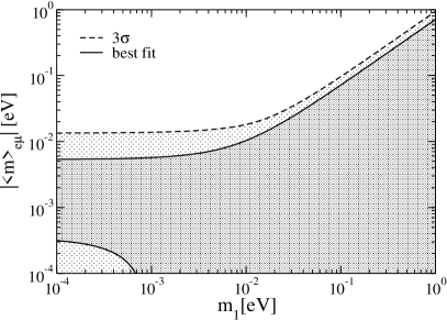
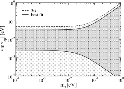
Figure 1: Allowed regions of the effective Majorana neutrino mass $|\langle m\rangle_{\mu e}|$ for normal (left panel) and inverted (right panel) hierarchy vs. the mass of lightest neutrino state: $m_{1}$ and $m_{3}$, respectively.

IV Neutrino mediated $(\mu^{-},e^{+})$ conversion. General formalism

The process of $(\mu^{-},e^{+})$ conversion is very similar to the $0\nu\beta\beta$-decay. Both processes violate lepton number by two units and, therefore, take place if and only if neutrinos are Majorana particles with non-zero mass.

On the other hand, there are various important differences between $(\mu^{-},e^{+})$ conversion and $0\nu\beta\beta$-decay. Among them we mention the following.

1. They have rather different available energies and different number of leptons in their final states. This results in a significant difference between the corresponding phase space integrals.

2. The emitted positron in $(\mu^{-},e^{+})$ conversion has large momentum and, therefore, the long-wave approximation is not valid in contrast to $0\nu\beta\beta$-decay.

3. As we will show, the nuclear matrix element of $(\mu^{-},e^{+})$ conversion for light neutrino-exchange demonstrates a singular behavior, absent in the $0\nu\beta\beta$-decay. This feature gives rise to the large imaginary part of the $(\mu^{-},e^{+})$ conversion amplitude. Technically the singularity significantly complicates the numerical calculation of the nuclear matrix elements.

4. In the case of the $(\mu^{-},e^{+})$ conversion there is large number of nuclear final states which must be properly taken into account.

Below, we analyze the amplitude of the $(\mu^{-},e^{+})$ conversion in nuclei mediated by light and heavy Majorana neutrinos. The corresponding diagrams are shown in Fig. 2. We concentrate only on the nuclear transition connecting the ground states ($g.s$) of the initial and final nuclei, which is favored from the experimental point of view due to the minimal background. The characteristic signature of $g.s\rightarrow g.s.$ transition is the presence of a peak in the $e^{+}$ spectrum at the energy

$$E_{e^{+}}=m_{\mu}-\varepsilon_{\mathrm{b}}-(E_{f}-E_{i})$$ (36)

which allows reliable separation of signal from background. Here, $m_{\mu}$, $\varepsilon_{b}$, $E_{i}$ and $E_{f}$ are the mass of muon, the muon atomic binding energy (for ${{}^{48}\mathrm{Ti}}$ this is $\varepsilon_{b}=1.45~{}\mathrm{MeV}$), the energies of initial and final nuclear ground states, respectively. Latter on we neglect the kinetic energy of final nucleus.

Figure 2: Direct (a) and cross (b) Feynman diagrams of $(\mu^{-},e^{+})$ conversion in nuclei mediated by Majorana neutrinos.

The leading order $(\mu^{-},e^{+})$ conversion matrix element, corresponding to the diagrams in Fig. 2, reads

$$\begin{split}\langle f|S^{(2)}|i\rangle&=-\mathrm{i}\left(\frac{G_{\mathrm{F}}}{\sqrt{2}}\right)^{2}\frac{1}{(2\pi)^{3/2}}\frac{1}{\sqrt{4E_{\mu^{-}}E_{e^{+}}}}\overline{v}(k_{e^{+}})(1+\gamma_{5})u(k_{\mu^{-}})\\ &\times\frac{m_{e}g^{2}_{\mathrm{A}}}{2\pi R}\left[\eta^{\mu e}_{\nu}{\cal M}^{(\mu e^{+})\Phi}_{\nu}+\eta^{\mu e}_{N}{\cal M}^{(\mu e^{+})\Phi}_{N}\right]2\pi\delta(E_{\mu^{-}}+E_{i}-E_{f}-E_{e^{+}}).\end{split}$$ (37)

Here $m_{e}$ and $m_{p}$ are electron and proton masses, $k_{e^{+}}$ ($E_{e^{+}}$), $k_{\mu^{-}}$ ($E_{\mu^{-}}$) are the momentum (energy) of outgoing positron and captured muon respectively. The conventional normalization factor involves the nuclear radius $R=1.1~{}A^{1/3}~{}{\mathrm{fm}}$. For the weak axial coupling constant $g_{A}$ we adopt the value $g_{A}=1.254$. In the above expression we introduced for convenience the following LNV parameters

$$\eta^{\mu e}_{\nu}=\frac{\langle m_{\nu}\rangle_{\mu e}}{m_{e}},\ \ \ \eta^{\mu e}_{N}=\langle M_{N}^{-1}\rangle_{\mu e}m_{p}.$$ (38)

The nuclear matrix elements in Eq. (37) defined as

$${\cal M}^{(\mu e^{+})\Phi}_{i}=-\frac{M^{(\mu e^{+})\Phi}_{\mathrm{F}({i})}}{g_{\mathrm{A}}^{2}}+M^{(\mu e^{+})\Phi}_{\mathrm{GT}(i)}\ \ \ \ \ \mbox{for}\ \qquad i=\nu,N$$ (39)

contain the Fermi $M^{(\mu e^{+})\Phi}_{\mathrm{F}}$ and Gamow-Teller $M^{(\mu e^{+})\Phi}_{\mathrm{GT}}$ contributions. They take the following form for the light Majorana neutrino exchange mechanism

$$\begin{split}M^{(\mu e^{+})\Phi}_{\mathrm{F}(\nu)}&=\frac{4\pi R}{(2\pi)^{3}}\int\frac{d\vec{q}}{2q}f^{2}_{\mathrm{V}}(\vec{q}^{\;2})\\ &\times\sum_{n}\left(\frac{\langle 0^{+}_{i}|\sum_{l}\tau^{+}_{l}\mathrm{e}^{-\mathrm{i}\vec{k}_{e^{+}}\cdot\vec{r}_{l}}\mathrm{e}^{-\mathrm{i}\vec{q}\cdot\vec{r}_{l}}|n\rangle\langle n|\sum_{m}\tau^{+}_{m}\mathrm{e}^{\mathrm{i}\vec{q}\cdot\vec{r}_{m}}\Phi(r_{m})|0^{+}_{f}\rangle}{q-E_{\mu^{-}}+E_{n}-E_{i}+\mathrm{i}\varepsilon_{n}}\right.\\ &+\left.\frac{\langle 0^{+}_{i}|\sum_{m}\tau^{+}_{m}\mathrm{e}^{\mathrm{i}\vec{q}\cdot\vec{r}_{m}}\Phi(r_{m})|n\rangle\langle n|\sum_{l}\tau^{+}_{l}\mathrm{e}^{-\mathrm{i}\vec{k}_{e^{+}}\cdot\vec{r}_{l}}\mathrm{e}^{-\mathrm{i}\vec{q}\cdot\vec{r}_{l}}|0^{+}_{f}\rangle}{q+E_{e^{+}}+E_{n}-E_{i}+\mathrm{i}\varepsilon_{n}}\right),\end{split}$$ (40)

$$\begin{split}M^{(\mu e^{+})\Phi}_{\mathrm{GT}(\nu)}&=\frac{4\pi R}{(2\pi)^{3}}\int\frac{d\vec{q}}{2q}f^{2}_{\mathrm{A}}(\vec{q}^{\;2})\\ &\times\sum_{n}\left(\frac{\langle 0^{+}_{i}|\sum_{l}\tau^{+}_{l}\vec{\sigma}_{l}\mathrm{e}^{-\mathrm{i}\vec{k}_{e^{+}}\cdot\vec{r}_{l}}\mathrm{e}^{-\mathrm{i}\vec{q}\cdot\vec{r}_{l}}|n\rangle\cdot\langle n|\sum_{m}\tau^{+}_{m}\vec{\sigma}_{m}\mathrm{e}^{\mathrm{i}\vec{q}\cdot\vec{r}_{m}}\Phi(r_{m})|0^{+}_{f}\rangle}{q-E_{\mu^{-}}+E_{n}-E_{i}+\mathrm{i}\varepsilon_{n}}\right.\\ &+\left.\frac{\langle 0^{+}_{i}|\sum_{m}\tau^{+}_{m}\vec{\sigma}_{m}\mathrm{e}^{\mathrm{i}\vec{q}\cdot\vec{r}_{m}}\Phi(r_{m})|n\rangle\cdot\langle n|\sum_{l}\tau^{+}_{l}\vec{\sigma}_{l}\mathrm{e}^{-\mathrm{i}\vec{k}_{e^{+}}\cdot\vec{r}_{l}}\mathrm{e}^{-\mathrm{i}\vec{q}\cdot\vec{r}_{l}}|0^{+}_{f}\rangle}{q+E_{e^{+}}+E_{n}-E_{i}+\mathrm{i}\varepsilon_{n}}\right).\end{split}$$ (41)

and for the heavy Majorana neutrino exchange mechanism

$$M^{(\mu e^{+})\Phi}_{I(N)}=\frac{4\pi R}{(2\pi)^{3}}\frac{2}{m_{p}m_{e}}\int{d\vec{q}}\langle 0^{+}_{i}|\sum_{lm}\tau^{+}_{l}\tau^{+}_{m}h_{I}(\vec{q}^{\;2})\mathrm{e}^{-\mathrm{i}\vec{q}\cdot(\vec{r}_{l}-\vec{r}_{m})}\mathrm{e}^{-\mathrm{i}\vec{k}_{e^{+}}\cdot\vec{r}_{l}}\Phi(r_{m})|0^{+}_{f}\rangle,\,(I=\mathrm{F,GT})$$ (42)

with

$$h_{\mathrm{F}}(\vec{q}^{\;2})=f_{\mathrm{V}}^{2}(\vec{q}^{\;2}),\qquad h_{\mathrm{GT}}(\vec{q}^{\;2})=\vec{\sigma}_{l}\cdot\vec{\sigma}_{m}f_{\mathrm{A}}^{2}(\vec{q}^{\;2}).$$ (43)

We use the conventional dipole parametrization for the nucleon form factors Towner and Hardy (1995)

$$f_{\mathrm{V}}(\vec{q}^{\;2})=\left(1+\frac{\vec{q}^{\;2}}{\Lambda_{\mathrm{V}}^{2}}\right)^{-2},\qquad f_{\mathrm{A}}(\vec{q}^{\;2})=\left(1+\frac{\vec{q}^{\;2}}{\Lambda_{\mathrm{A}}^{2}}\right)^{-2},$$ (44)

with $\Lambda_{\mathrm{V}}=0.71~{}\mathrm{GeV}$, $\Lambda_{\mathrm{A}}=1.09~{}\mathrm{GeV}$. In Eqs. (40)-(42) the factor $\Phi(r)$ is the radial part of the bound muon 1S wave function (see Appendix A). In the denominators of Eqs. (40), (41) we introduced the widths $\varepsilon_{n}$ of intermediate nuclear states.

In the calculations of nuclear matrix elements we adopt the following approximations.

1. Taking into account slow variation of muon wave function within the nucleus we apply the standard approximation Kosmas et al. (1994)

   $$|{\cal M}^{(\mu e^{+})\Phi}_{i}|^{2}=\langle\Phi\rangle^{2}|{\cal M}_{i}^{(\mu e^{+})}|^{2},\quad i=\nu,N.$$ (45)

   Here $\langle\Phi\rangle^{2}$ is the muon average probability density and

   $$\left|{\cal M}_{i}^{(\mu e^{+})}\right|=\left|{\cal M}^{(\mu e^{+})\Phi}_{i}\right|_{\Phi=1}\ .$$ (46)

   The explicit form of $\langle\Phi\rangle^{2}$ is given in Appendix B.

2. In muon to positron conversion the typical energy of light intermediate neutrinos is about 100 MeV ($\omega\approx|q|\geq 1/R\sim 100~{}MeV$) which is much larger than the typical excitation energies of intermediate nuclear states. Therefore, to a good approximation the individual energies of these states in the energy denominators of Eqs. (40), (41) can be neglected or replaced by some average value $<E_{n}>$ to which the matrix elements are not very sensitive. Then the intermediate nuclear states can be summed up by closure. A similar situation occurs in the case of $0\nu\beta\beta$-decay Doi et al. (1985); Faessler and Šimkovic (1998); Suhonen and Civitarese (1998).

   Thus, in Eqs. (40), (41) we complete the sum over the virtual intermediate nuclear states by closure after replacing $E_{n}$, $\varepsilon_{n}$ with some average values $\langle E_{n}\rangle$, $\varepsilon$, respectively:

   $$\sum_{n}\frac{|n\rangle\langle n|}{q-E_{\mu^{-}}+E_{n}-E_{i}+\mathrm{i}\varepsilon_{n}} \approx\frac{1}{q-E_{\mu^{-}}+\langle E_{n}\rangle-E_{i}+\mathrm{i}\varepsilon},$$ (47)

   $$\sum_{n}\frac{|n\rangle\langle n|}{q+E_{e^{+}}+E_{n}-E_{i}+\mathrm{i}\varepsilon_{n}} \approx\frac{1}{q+E_{e^{+}}+\langle E_{n}\rangle-E_{i}+\mathrm{i}\varepsilon}.$$ (48)

Obviously, the validity of the closure approximation is just the question of the choice of the average excitation energy which will be discussed in Section V.

The angular part of neutrino propagators can be integrated using the relation

$$\int\mathrm{e}^{-\mathrm{i}\vec{q}\cdot(\vec{r}_{l}-\vec{r}_{m})}\mathrm{e}^{-\mathrm{i}\vec{k}_{e^{+}}\cdot\vec{r}_{l}}d\Omega_{q}=\\ (4\pi)^{2}\sum_{\lambda}(-1)^{\lambda}\sqrt{2\lambda+1}\,\mathrm{j}_{\lambda}(k_{e^{+}}R_{lm})\mathrm{j}_{0}(qr_{lm})\mathrm{j}_{\lambda}(k_{e^{+}}r_{lm}/2)\left\{\mathrm{Y}_{\lambda}(\Omega_{r_{lm}})\otimes\mathrm{Y}_{\lambda}(\Omega_{R_{lm}})\right\}_{00},$$ (49)

Where $\mathrm{j}_{\lambda}$ is the spherical Bessel function, $\mathrm{Y}_{\lambda}$ is the spherical harmonic and

$${\vec{r}}_{ij}={\vec{r}}_{i}-{\vec{r}}_{j},\qquad r_{ij}=|{\vec{r}}_{ij}|,\qquad{\vec{R}}_{ij}=\frac{{\vec{r}}_{i}+{\vec{r}}_{j}}{2},\qquad R_{ij}=|{\vec{R}}_{ij}|.$$ (50)

Note that in the limit when the outgoing positron momentum $|\vec{k}_{e^{+}}|$ is zero the right hand side of Eq. (49) is reduced to $4\pi\mathrm{j}_{0}(qr_{lm})$.

With the above approximations and comments we can write down the expressions for the nuclear matrix elements introduced in Eq. (46) in the form

$${\cal M}_{\nu}^{(\mu e^{+})}=M_{\mathrm{dir.}}^{(\mu e^{+})}+M_{\mathrm{cro.}}^{(\mu e^{+})},\ \ \ \ \ {\cal M}_{N}^{(\mu e^{+})}=-\frac{M_{\mathrm{F}(N)}^{(\mu e^{+})}}{g_{\mathrm{A}}^{2}}+M_{\mathrm{GT}(N)}^{(\mu e^{+})}.$$ (51)

Here the nuclear matrix element ${\cal M}_{\nu}^{(\mu e^{+})}$ is decomposed into the contributions coming from direct and cross Feynman diagrams in Fig 2. They can be written as

$$\begin{split}M_{\mathrm{dir.}}^{(\mu e^{+})}&=\langle 0^{+}_{i}|\sum_{lm}\tau^{+}_{l}\tau^{+}_{m}4\pi\sum_{\lambda}(-1)^{\lambda}\sqrt{2\lambda+1}\mathrm{j}_{\lambda}(k_{e^{+}}R_{lm})\mathrm{j}_{\lambda}\left(\frac{k_{e^{+}}r_{lm}}{2}\right)\left\{\mathrm{Y}_{\lambda}(\Omega_{r_{lm}})\otimes\mathrm{Y}_{\lambda}(\Omega_{R_{lm}})\right\}_{00}\\ &\times\frac{R}{\pi}\int_{0}^{\infty}\frac{\mathrm{j}_{0}(qr_{lm})}{q-E_{\mu^{-}}+\langle E_{n}\rangle-E_{i}+\mathrm{i}\varepsilon}\left(\vec{\sigma_{l}}\cdot\vec{\sigma_{m}}f_{\mathrm{A}}^{2}(q^{2})-\frac{f_{\mathrm{V}}^{2}(q^{2})}{g^{2}_{\mathrm{A}}}\right)qdq|0^{+}_{f}\rangle,\\ \end{split}$$ (52)

$$\begin{split}M_{\mathrm{cro.}}^{(\mu e^{+})}&=\langle 0^{+}_{i}|\sum_{lm}\tau^{+}_{l}\tau^{+}_{m}4\pi\sum_{\lambda}(-1)^{\lambda}\sqrt{2\lambda+1}\,\mathrm{j}_{\lambda}(k_{e^{+}}R_{lm})\mathrm{j}_{\lambda}\left(\frac{k_{e^{+}}r_{lm}}{2}\right)\left\{\mathrm{Y}_{\lambda}(\Omega_{r_{lm}})\otimes\mathrm{Y}_{\lambda}(\Omega_{R_{lm}})\right\}_{00}\\ &\times\frac{R}{\pi}\int_{0}^{\infty}\frac{\mathrm{j}_{0}(qr_{lm})}{q+E_{e^{+}}+\langle E_{n}\rangle-E_{i}+\mathrm{i}\varepsilon}\left(\vec{\sigma_{l}}\cdot\vec{\sigma_{m}}f_{\mathrm{A}}^{2}(q^{2})-\frac{f_{\mathrm{V}}^{2}(q^{2})}{g^{2}_{\mathrm{A}}}\right)qdq|0^{+}_{f}\rangle.\end{split}$$ (53)

The Gamow-Teller and Fermi nuclear matrix elements of heavy Majorana neutrino exchange mechanism take the form

$$\begin{split}M_{I(N)}^{(\mu e^{+})}&=\frac{1}{m_{p}m_{e}}\langle 0^{+}_{i}|\sum_{lm}\tau^{+}_{l}\tau^{+}_{m}4\pi\sum_{\lambda}(-1)^{\lambda}\sqrt{2\lambda+1}\,\mathrm{j}_{\lambda}(k_{e^{+}}R_{lm})\mathrm{j}_{\lambda}\left(\frac{k_{e^{+}}r_{lm}}{2}\right)\\ &\times\left\{\mathrm{Y}_{\lambda}(\Omega_{r_{lm}})\otimes\mathrm{Y}_{\lambda}(\Omega_{R_{lm}})\right\}_{00}\frac{2R}{\pi}\int_{0}^{\infty}\mathrm{j}_{0}(qr_{lm})h_{I}(\vec{q}^{\;2})q^{2}dq|0^{+}_{f}\rangle\quad(I=\mathrm{F,GT}),\end{split}$$ (54)

with $h_{I}(\vec{q}^{\;2})$ defined in Eq. (43).

It is important to note that the value of $E_{r}\equiv-E_{\mu^{-}}+\langle E_{n}\rangle-E_{i}$ is negative for the studied nuclear system $A=48$. Therefore, the contribution of direct Feynman diagram in Fig. 2a with the light intermediate neutrino has the pole at $q=-E_{r}-i\varepsilon$, as it follows from the formula (52). As a consequence, the imaginary part of the $(\mu^{-},e^{+})$ conversion amplitude for the case of the light neutrino exchange can be significant. This fact was first noticed in Ref. Šimkovic et al. (2001) and then in Refs. Divari et al. (2001, 2002). In Ref. Divari et al. (2002) it was shown that the imaginary part of the amplitude dominates in the total branching ratio of the $(\mu^{-},e^{+})$ conversion in ²⁷Al. In the next section we will demonstrate that the similar conclusion is valid for $(\mu^{-},e^{+})$ conversion in ⁴⁸Ti.

The following comment is in order. In the expressions (40)-(42) for nuclear matrix elements ${\cal M}^{(\mu e^{+})\Phi}_{i}$ we neglected the contributions of the higher order terms of nucleon current (weak-magnetism, induced pseudoscalar coupling). As suggested by the analogy with $0\nu\beta\beta$-decay  Simkovic et al. (1999), these terms should not be essential for the light neutrino exchange mechanism meanwhile their contribution in the case of heavy Majorana neutrino exchange might be significant. However, the detailed study of this effect is beyond the scope of this paper and will be considered elsewhere.

Now we are ready to write down the expression for $g.s.\rightarrow g.s.$ $(\mu^{-},e^{+})$ conversion rate. For simplicity we assume that only one mechanism is in operation and present the corresponding rates for light and heavy Majorana neutrino exchange mechanisms separately:

$$\Gamma_{i}^{(\mu e^{+})}=\frac{1}{\pi}E_{e^{+}}~{}k_{e^{+}}F(Z-2,E_{e^{+}})c_{\mu e}\langle\Phi\rangle^{2}|{\cal M}_{i}^{(\mu e^{+})}|^{2}|\eta_{i}^{(\mu e)}|^{2},\qquad(i=\nu,N)$$ (55)

where $c_{\mu e}=2G_{\mathrm{F}}^{4}[({m_{e}m_{\mu}})/{(4\pi m_{\mu}R)}]^{2}g_{\mathrm{A}}^{4}$, $k_{e^{+}}=|{\vec{k}}_{e^{+}}|$. The relativistic Coulomb factor $F(Z,E)$ in Eq. (55) we take in the standard form  Doi et al. (1985)

$$F(Z,E)=\left[\frac{2}{\Gamma(2\gamma_{1}+1)}\right]^{2}(2pR)^{2(\gamma_{1}-1)}|\Gamma(\gamma_{1}-\mathrm{i}y)|^{2}e^{-\pi y},$$ (56)

where $\gamma_{1}=\sqrt{1-(\alpha Z)^{2}}$, $\alpha$ is the fine structure constant, $y=\alpha ZE/p$.

To conclude this section we point out that in our analysis of $(\mu^{-},e^{+})$ conversion we limit ourselves by the $0^{+}_{g.s.}\rightarrow 0^{+}_{g.s.}$ transition which represents a particular contribution to the total rate of this process. This is the most favored channel for experimental study since its signal can be reliably separated from the background as we commented above. On the other hand in Ref. Divari et al. (2002) it was demonstrated that $0^{+}_{g.s.}\rightarrow 0^{+}_{g.s.}$ transition constitutes about $41\%$ of the total $(\mu^{-},e^{+})$ conversion rate in ²⁷Al and, therefore neglecting the excited final states is a reasonable approximation. We expect that this conclusion holds for ⁴⁸Ti as well.

V Nuclear matrix elements

We calculate the $(\mu^{-},e^{+})\$conversion nuclear matrix elements within the proton-neutron renormalized Quasiparticle Random Phase Approximation (pn-RQRPA) Toivanen and Suhonen (1995); Schwieger et al. (1996); Faessler et al. (1997); Wodecki et al. (1999). In the present study we focus on ⁴⁸Ti nucleus utilized as a stopping target in SINDRUM II Dohmen et al. (1993) and PRIME Kuno (2001) experiments.

Nuclear transition scheme for the studied $A=48$ nuclear system is shown in Fig. 3

Figure 3: Transition scheme for the $A=48$ nuclear system.

Our nuclear structure calculations involve the single-particle model space both for protons and neutrons consisting of the full $0-3\hbar\omega$ shells plus $2s_{1/2}$, $0g_{7/2}$ and $0g_{9/2}$ levels. The single particle energies were obtained using the Coulomb–corrected Woods–Saxon potential. The two-body G-matrix elements were calculated from the Bonn one-boson exchange potential on the basis of the Brueckner theory. Since the considered model space is finite the pairing interactions have been adjusted to fit the empirical pairing gaps Cheoun et al. (1993a). In addition, we renormalize the particle-particle and particle-hole channels of the G-matrix interaction of the nuclear Hamiltonian $H$ by introducing the parameters $g_{pp}$ and $g_{ph}$, respectively. The two-nucleon correlation effect has been taken into account in a standard way by multiplying the operators with the square of the correlation Jastrow-like function Miller and Spencer (1976). The details of our nuclear model can be found in Appendix C

As we already commented in section IV the matrix element of the direct contribution (Fig. 2a) of light neutrino exchange mechanism contains an imaginary part which stems from the pole of the integrand in Eq. (52) at $q=-E_{r}-i\varepsilon$. Taking into account that the widths $\varepsilon$ of low lying nuclear states are negligible in comparison with their energies one can separate the imaginary and real parts of this matrix element using the well known formula

$$\frac{1}{\alpha+\mathrm{i}\varepsilon}={\cal{P}}\frac{1}{\alpha}-\mathrm{i}\pi\delta(\alpha)$$ (57)

valid in the limit $\varepsilon\rightarrow 0$.

Table 1: Nuclear matrix elements of the light and heavy Majorana neutrino exchange mechanisms of $(\mu^{-},e^{+})$ conversion in ⁴⁸Ti [see Eqs. (51)-(54)]. The calculations have been performed within pn-RQRPA without and with the inclusion of two-nucleon short-range correlations (s.r.c.).

$g_{pp}$	$M_{\mathrm{cro.}}^{(\mu e^{+})}$	$\mathrm{Re}(M_{\mathrm{dir.}}^{(\mu e^{+})})$	$\mathrm{Im}(M_{\mathrm{dir.}}^{(\mu e^{+})})$	$|{\cal M}_{\nu}^{(\mu e^{+})}|$	$|{\cal M}_{N}^{(\mu e^{+})}|$
without s.r.c.
0.8	0.097	0.002	0.088	0.132	25.5
1.0	0.077	0.034	0.059	0.125	22.8
1.2	0.051	0.091	0.018	0.142	19.6
with s.r.c.
0.8	0.049	-0.080	0.050	0.059	5.92
1.0	0.034	-0.040	0.024	0.025	5.19
1.2	0.013	0.027	-0.013	0.042	4.33
with s.r.c., $|\vec{k}_{e^{+}}|=0$
0.8	0.298	-0.029	0.386	0.470	31.4
1.0	0.233	0.069	0.275	0.408	27.7
1.2	0.147	0.243	0.125	0.409	23.2

In Table 1 we show the nuclear matrix elements of light and heavy Majorana neutrino exchange mechanisms of the $(\mu^{-},e^{+})$ conversion in ${{}^{48}\mathrm{Ti}}$ calculated for $g_{pp}=1.0$ and $g_{pp}=0.8,~{}1.0,~{}1.2$. All the presented results were obtained for the particular value of energy difference $\langle E_{n}\rangle-E_{i}=10~{}\mathrm{MeV}$. This choice is justified by weak dependence of the matrix elements on this parameter within the interval of its reasonable values $2~{}\mathrm{MeV}\leq(\langle E_{n}\rangle-E_{i})\leq 15~{}\mathrm{MeV}$. We verified this property by the direct numerical analysis. In Fig. 4 we present the absolute value of the light neutrino exchange nuclear matrix element $|M^{(\mu e^{+})}|$ as a function of the average value $\langle E_{n}\rangle-E_{i}$ for $g_{pp}=0.8$, 1.0 and 1.2. One can see that its variation within the studied range of $\langle E_{n}\rangle-E_{i}$ is about 30%. For $g_{pp}=0.8$, $1.0$ ($g_{pp}=1.2$) the matrix element is an increasing (decreasing) function of $\langle E_{n}\rangle-E_{i}$. Different behavior in these two cases is related to a specific interplay between the direct $M_{\mathrm{dir.}}^{(\mu e^{+})}$ and cross $M_{\mathrm{cro.}}^{(\mu e^{+})}$ diagram terms in $M^{(\mu e^{+})}$. For $g_{pp}=0.8$, $1.0$ there is a mutual cancellation of the real parts of these two terms so that the imaginary part of $M_{\mathrm{dir.}}^{(\mu e^{+})}$, which is a growing function of $\langle E_{n}\rangle-E_{i}$, dominantes and determines the behavior of $M^{(\mu e^{+})}$. For $g_{pp}=1.2$ the situation is opposite. The real parts, decreasing with $\langle E_{n}\rangle-E_{i}$, contribute coherently and constitute the dominant part of $M^{(\mu e^{+})}$ which becomes a decreasing function of $\langle E_{n}\rangle-E_{i}$.

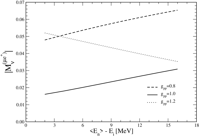
Figure 4: The nuclear matrix elements of the light Majorana neutrino exchange mechanisms of the $(\mu^{-},e^{+})$ conversion in ${}^{48}Ti$ as a function of the average value of energy difference $<E_{n}>-E_{i}$.

We have also found that the nuclear matrix elements do not show an appreciable variation in the physical region of the parameter $g_{ph}$ ($0.8\leq g_{ph}\leq 1.2$). On the contrary, as seen from Table 1 they significantly depend on the renormalization parameter $g_{pp}$ and on the two-nucleon short-range correlation. It is also worth noting that the large momentum $k_{e^{+}}$ of outgoing positron is the source of strong suppression of the $(\mu^{-},e^{+})$ conversion matrix elements. In order to illustrate this effect we presented in Table 1 the matrix elements calculated in the limit $|k_{e^{+}}|=0$ when the suppression of this type is absent. The cross check of Table 1 reveals the corresponding suppression factor of about $\sim 10$.

An important issue of our analysis is the presence of the significant imaginary part of matrix element ${\cal M}_{\nu}^{\mu e^{+}}$ corresponding to the light Majorana neutrino exchange mechanism. This fact was first noticed in Ref. Šimkovic et al. (2001) and then in Refs. Divari et al. (2001, 2002). In the previous studies of $(\mu^{-},e^{+})$ conversion Doi et al. (1985); Kamal and Ng (1979); Vergados (1981); Leontaris and Vergados (1983) the role of imaginary part was overlooked.

In the presented detailed study we have found, that the relative contribution of the imaginary part to the rate of $(\mu^{-},e^{+})$ conversion in ⁴⁸Ti is always significant but appreciably depends on the value of the nuclear model parameter $g_{pp}$ and on the short range correlations. It absolutely dominates over the real part by the factor of $\sim 16$ for the most conventional case when $g_{pp}=1$ and the short range correlations are taken into account (for the motivation of this choice see, for instance, Ref. Rodin et al. (2003); Bilenky et al. (2004)). This conclusion is consistent with the result of Ref. Divari et al. (2002) studying $(\mu^{-},e^{+})$ conversion in ${{}^{27}\mathrm{Al}}$ within shell-model approach where it was found that the imaginary part for the light neutrino exchange dominates over the real one by the factor of about $~{}20$. However it is notable that the relative contribution of the imaginary part is model dependent and can vary from one nucleus to another. In this situation the role of the imaginary part in $(\mu^{-},e^{+})$ conversion requires further study for other nuclear systems.

From the view point of nuclear structure theory it is instructive to compare the values of $(\mu^{-},e^{+})\$conversion nuclear matrix elements with the corresponding values of $0\nu\beta\beta$-decay matrix elements of $\mathrm{A}=48$ nuclear system. For $0\nu\beta\beta$-decay this system is represented by ⁴⁸Ca with the matrix elements

$$|{\cal M}_{\nu}^{(ee)}|=0.82,\quad|{\cal M}_{N}^{(ee)}|=24.2$$ (58)

derived within the pn-RQRPA approach in Ref. Simkovic et al. (2002a). As seen, the matrix elements of the $(\mu^{-},e^{+})$ conversion (60) are strongly suppressed in comparison with those of $0\nu\beta\beta$-decay (58) by the factors of about $17$ and  $5$ for the light and heavy Majorana neutrino exchange mechanisms respectively. As we commented above the explanation of this difference between the two processes mostly resides in the large momentum of outgoing positron produced in $(\mu^{-},e^{+})$ conversion.

VI $(\mu^{-},e^{+})$ conversion and effective neutrino masses

Now, let us discuss the possible issues of $(\mu^{-},e^{+})\$conversion experiments for neutrino physics.

From Eq. (55) we obtain the $(\mu^{-},e^{+})\$conversion branching ratios in ⁴⁸Ti for the light and heavy Majorana neutrino exchange mechanisms:

$$R^{(\mu e^{+})}_{i}\equiv\frac{\Gamma_{i}^{(\mu e)}}{\Gamma^{(\mu\nu)}}=2.6\times 10^{-22}|{\cal M}^{(\mu e)}_{i}|^{2}|\eta_{i}^{(\mu e)}|^{2}\quad(i=\nu,N).$$ (59)

Here we use the known experimental value $\Gamma^{(\mu\nu)}=2.60\times 10^{6}~{}\mathrm{s}^{-1}$ Suzuki et al. (1987) of ordinary muon capture rate in ⁴⁸Ti. For the further discussion we choose the following sample values of nuclear matrix elements of ⁴⁸Ti from Table 1

$$|{\cal M}_{\nu}^{(\mu e^{+})}|=0.025,\quad|{\cal M}_{N}^{(\mu e^{+})}|=5.2$$ (60)

corresponding to $g_{pp}=1.0$ with the presence of the two-nucleon short range correlations.

Substituting these numerical values of nuclear matrix elements to Eq. (59) we obtain

$$R^{(\mu e^{+})}_{\nu} =1.6~{}10^{-25}\times\frac{|{\langle m\rangle_{\mu e}}|^{2}}{m_{e}^{2}},$$ (61)

$$R^{(\mu e^{+})}_{N} =7.0~{}10^{-21}\times|\langle M_{N}^{-1}\rangle_{\mu e}|^{2}m_{p}^{2}.$$ (62)

From the existing experimental upper bound in Eq. (2) one obtains the following limits for the effective masses of light and heavy Majorana neutrinos

$$|{\langle m\rangle_{\mu e}}|\leq 1.3\times 10^{6}~{}\mbox{MeV}\ \ \ \ \ \ \ \ \ \ |\langle M_{N}^{-1}\rangle_{\mu e}|^{-1}\geq 3.3\times 10^{-2}~{}\mbox{MeV}$$ (63)

Obviously, these limits have no physical sense since they do not satisfy the consistency condition in Eq. (16) with the characteristic energy scale $q_{0}\sim m_{\mu}=105$MeV of $(\mu^{-},e^{+})\$conversion. Meaningful limits on the parameters ${\langle m\rangle_{\mu e}}$, $\langle M_{N}^{-1}\rangle_{\mu e}$, which may have some impact on neutrino physics, could be reached if the $(\mu^{-},e^{+})\$conversion experiments would improve their sensitivities by at least 10 orders of magnitude. Clearly, such a tremendous improvement is unrealistic for the near future experiments.

On the other hand we can estimate the expected branching ratios of $(\mu^{-},e^{+})\$conversion induced by the light and heavy Majorana neutrino exchange using the estimates of ${\langle m\rangle_{\mu e}}$, $\langle M_{N}^{-1}\rangle_{\mu e}$ made in section III from the present neutrino data. Substituting the values of these parameters in Eqs. (61)-(62) we obtain the following results.

Light Majorana neutrino exchange contribution:

1. Normal neutrino mass hierarchy, $|<m>_{\mu e}|\simeq(0.35-5.3)\times 10^{-3}~{}\text{eV}$

   $$R^{(\mu e^{+})}_{\nu}\simeq(0.008-1.7)\times 10^{-41}.$$ (64)

2. Inverted neutrino mass hierarchy, $|<m>_{\mu e}|\simeq(0.3-3.3)\times 10^{-2}~{}\text{eV}$

   $$R^{(\mu e^{+})}_{\nu}\simeq(0.05-6.7)\times 10^{-40}.$$ (65)

3. Quasidegenerate mass hierarchy

   $$R^{(\mu e^{+})}_{\nu}\lesssim 1.3\times 10^{-36},\quad\langle m_{\nu}\rangle<1.46~{}\mathrm{eV},~{}\text{Troitsk ${{}^{3}\mathrm{H}}$ experiment~{}\cite[cite]{\@@bibref{Authors Phrase1YearPhrase2}{Troitsk}{\@@citephrase{(}}{\@@citephrase{)}}}}$$ (66)

   $$R^{(\mu e^{+})}_{\nu}\lesssim 1.5\times 10^{-36},\quad\langle m_{\nu}\rangle<1.56~{}\mathrm{eV},~{}\text{Mainz ${{}^{3}\mathrm{H}}$ experiment~{}\cite[cite]{\@@bibref{Authors Phrase1YearPhrase2}{wei03}{\@@citephrase{(}}{\@@citephrase{)}}}}$$ (67)

   $$R^{(\mu e^{+})}_{\nu}\lesssim 1.6\times 10^{-38},\quad\langle m_{\nu}\rangle<0.16~{}\mathrm{eV},~{}\text{Cosmological data~{}\cite[cite]{\@@bibref{Authors Phrase1YearPhrase2}{spe03}{\@@citephrase{(}}{\@@citephrase{)}}}}$$ (68)

   $$R^{(\mu e^{+})}_{\nu}\sim 1.3\times 10^{-38},\quad\langle m_{\nu}\rangle\sim 0.14~{}\mathrm{eV},~{}\text{Cosmological data~{}\cite[cite]{\@@bibref{Authors Phrase1YearPhrase2}{all03}{\@@citephrase{(}}{\@@citephrase{)}}}}$$ (69)

Let us remind that the cosmological data based limits (68)and (69), albeit more stringent, are more model dependent than the laboratory ones (66) and (67).

Heavy Majorana neutrino contribution:

$$R^{(\mu e^{+})}_{N}\leq 3.8\times 10^{-24}$$ (70)

All the values of $(\mu^{-},e^{+})\$conversion branching ratio in Eq. (64)-(70) are hopelessly low for being detected even in a distant future. Thus, searching for $(\mu^{-},e^{+})\$conversion cannot have any direct impact on neutrino physics. On the other hand any observation of $(\mu^{-},e^{+})\$conversion at branching ratios above the limits in Eq. (64)-(70) would be unambiguous signal of new physics beyond the simplest extension of SM with massive Majorana neutrinos and would imply the presence of new interactions.

This conclusion are in a sharp contrast with $0\nu\beta\beta$-decay experiments which already provide an important information on neutrino properties and are expected to detect neutrino contribution in the near future. This is due to their unique sensitivities to $0\nu\beta\beta$-decay signal. In order to give an impression to which extent $0\nu\beta\beta$-decay experiments overcome in sensitivities the experiments searching for $(\mu^{-},e^{+})\$conversion let us compare, as an example, the rates of $(\mu^{-},e^{+})$ conversion in ⁴⁸Ti and $0\nu\beta\beta$-decay of ${{}^{48}\mathrm{Ca}}$. To this end it is sufficient to consider only light Majorana neutrino exchange contributions in both cases. For the rate of $0\nu\beta\beta$-decay we have the well known formula

$$\Gamma^{(ee)}_{\nu}=\ln 2G_{01}\left|\frac{\langle m_{\nu}\rangle_{ee}}{m_{e}}\right|^{2}|{\cal M}^{(ee)}_{\nu}|^{2},$$ (71)

where $G_{01}=8.031\times 10^{-14}~{}\mathrm{year}^{-1}$ Pantis et al. (1996) and

$$\langle m_{\nu}\rangle_{ee}=\sum\limits_{k=\mathrm{light}}(U_{ek})^{2}m_{k}.$$ (72)

Using the value of $0\nu\beta\beta$-decay nuclear matrix element ${\cal M}^{(ee)}_{\nu}$ from Eq. (58) we estimate the ratio of $(\mu^{-},e^{+})\$conversion to $0\nu\beta\beta$-decay rates:

$$\frac{\Gamma_{\nu}^{(\mu e^{+})}}{\Gamma_{\nu}^{(ee)}}=9.7\times 10^{4}\times\frac{|{\cal M}^{(\mu e)}_{\nu}|^{2}}{|{\cal M}^{(ee)}_{\nu}|^{2}}\left|\frac{\langle m_{\nu}\rangle_{\mu e}}{\langle m_{\nu}\rangle_{ee}}\right|^{2}=351\left|\frac{\langle m_{\nu}\rangle_{\mu e}}{\langle m_{\nu}\rangle_{ee}}\right|^{2}.$$ (73)

The the $(\mu^{-},e^{+})$ conversion receives a significant enhancement mostly due to the larger available energy of this process. Thus, for ${\langle m_{\nu}\rangle_{\mu e}}\sim\langle m_{\nu}\rangle_{ee}$ the $(\mu^{-},e^{+})\$conversion rate ${\Gamma_{\nu}^{(\mu e^{+})}}$ is by more than 2 orders of magnitude larger than the rate ${\Gamma_{\nu}^{(ee)}}$ of $0\nu\beta\beta$-decay. Nevertheless the experimental prospects for searching for $0\nu\beta\beta$-decay are incomparably better than those for $(\mu^{-},e^{+})\$conversion. This is mainly because the number of potentially $0\nu\beta\beta$-decaying nuclei monitored in $0\nu\beta\beta$ experiments is by many orders of magnitude larger than the number of mesoatoms created by muon beams in the muon-conversion experiments.

VII Summary and outlook

In summary, the light and heavy Majorana neutrino exchange mechanisms of $(\mu^{-},e^{+})$ conversion have been studied. Special emphasis was made on the nuclear structure aspects of this process. We have performed the first realistic calculations of the corresponding nuclear matrix elements for ⁴⁸Ti nucleus used as a stopping target in the current Dohmen et al. (1993) and the forthcoming Kuno (2001) $(\mu^{-},e^{+})\$conversion experiments. Our analysis is based on the pn-RQRPA approach and limited to the case of $0^{+}_{g.s.}\rightarrow 0^{+}_{g.s.}$ transition channel, which is most relevant for experimental searches for $(\mu^{-},e^{+})\$conversion. The effects of the ground state and two-nucleon short-range correlations have been properly taken into account. We pointed out that their inclusion results in the significant reduction of $(\mu^{-},e^{+})$ conversion matrix elements.

Our detailed analysis confirmed the conjecture of Refs. Šimkovic et al. (2001); Divari et al. (2001) on the importance of the imaginary part of the nuclear matrix elements for the case of the light Majorana neutrino exchange mechanism of $(\mu^{-},e^{+})\$conversion. The similar result was recently obtained in Ref. Divari et al. (2002) for $(\mu^{-},e^{+})\$conversion in ²⁷Al.

We also derived the limits on the effective masses of light ${\langle m\rangle_{\mu e}}$ and heavy $\langle M_{N}^{-1}\rangle_{\mu e}$ Majorana neutrinos from the neutrino oscillations, tritium beta decay, accelerator and cosmological data. Using these limits we estimated the expected rates of $(\mu^{-},e^{+})\$conversion induced by Majorana neutrino exchange. Their values were found to be so small that even within a quite distant future the $(\mu^{-},e^{+})\$conversion experiments will hardly be able to detect the neutrino contribution and, thus, to have a direct impact on neutrino physics. On the other hand the eventual observation of $(\mu^{-},e^{+})\$conversion at larger rates would be unambiguous signal of new physics beyond the standard model implying new non-standard interactions. Moreover, this observation, independently of the $(\mu^{-},e^{+})\$conversion rate, would definitely prove that neutrinos are Majorana particles as follows from the “black box” type theorem Schechter and Valle (1982) establishing the fundamental relation between LNV processes and Majorana nature of neutrinos. In view of this it remains actual to study possible scenarios of new physics consistent with the values of $(\mu^{-},e^{+})\$conversion rates within the reach of the present and near future experiments.

Appendix A Bound muon wave-function

The bound muon wave function (1S-state) is given by the expression

$$\Psi(x)=\Phi(r)e^{-\mathrm{i}E_{\mu^{-}}x_{0}}\frac{u_{\mu}^{s}}{\sqrt{2E_{\mu^{-}}}},$$ (74)

where the radial $\Phi(r)$ and the spinorial $u_{\mu}^{s}$ parts have the forms

$$\Phi(r)=\frac{Z^{3/2}}{(\pi a_{\mu}^{3})^{1/2}}e^{-Zr/a_{\mu}}$$ (75)

and

$$u^{s}_{\mu}=\sqrt{2E_{\mu^{-}}}\begin{pmatrix}\chi^{s}\\ 0\end{pmatrix},$$ (76)

with $a_{\mu}=4\pi/(m_{\mu}e^{2})$ ($a_{\mu}/a_{e}\approx m_{e}/m_{\mu}\approx 5\times 10^{-3}$), $m_{\mu}$ is reduced mass of muon atom, $Z$ is nuclear charge.

Appendix B Muon average probability density over nucleus

Muon average probability density over nucleus is defined as

$$\langle\Phi\rangle^{2}\equiv\frac{\int|\Phi(\vec{x})|^{2}\rho(\vec{x})d^{3}x}{\int\rho(\vec{x})d^{3}x},$$ (77)

where $\rho(\vec{x})$ is the nuclear charge density. To a good approximation it can be written in the following compact form Kosmas et al. (1994)

$$\langle\Phi\rangle^{2}=\frac{\alpha^{3}m_{\mu}^{3}}{\pi}\frac{Z_{\mathrm{eff}}^{4}}{Z}.$$ (78)

Here the effective charge for $Z=22$ nuclear system is $Z_{\mathrm{eff}}$ is $Z_{\mathrm{eff}}=17.5$  Kosmas et al. (1994).

Appendix C Nuclear Model

Here we shortly outline our approach to the nuclear structure calculations.

We introduce particle (quasiparticle) creation operators as $c^{\dagger}_{\tau m_{\tau}}$ ($a^{\dagger}_{\tau m_{\tau}}$) for $\tau=p,n$. The indices $p\equiv(n_{p},l_{p},j_{p})$ and $n\equiv(n_{n},l_{n},j_{n})$ denote proton and neutron quantum numbers in a particular shell. Transformation from the particle to quasiparticle basis is realized by the Bogolyubov transformation

$$\begin{pmatrix}c^{\dagger}_{\tau m_{\tau}}\\ \tilde{c}_{\tau m_{\tau}}\end{pmatrix}=\begin{pmatrix}u_{\tau}&-v_{\tau}\\ v_{\tau}&u_{\tau}\end{pmatrix}\begin{pmatrix}a^{\dagger}_{\tau m_{\tau}}\\ \tilde{a}_{\tau m_{\tau}}\end{pmatrix}$$ (79)

where the tilde denotes time reversal, $\tilde{a}_{\tau m_{\tau}}=(-1)^{j_{\tau}-m_{\tau}}a_{\tau\,-m_{\tau}}$.

Occupation amplitudes $u_{\tau}$, $v_{\tau}$ and quasiparticle energies $E_{\tau}$ are obtained by solving BCS equation Cheoun et al. (1993b)

$$\begin{pmatrix}\varepsilon_{\tau}-\lambda_{\tau}&\Delta_{\tau}\\ \Delta_{\tau}&-\varepsilon_{\tau}+\lambda_{\tau}\end{pmatrix}\begin{pmatrix}u_{\tau}\\ v_{\tau}\end{pmatrix}=E_{\tau}\begin{pmatrix}u_{\tau}\\ v_{\tau}\end{pmatrix},$$ (80)

where $\varepsilon_{\tau}$ is the energy of single particle state derived from the Wood–Saxon potential. The pairing potential takes the form

$$\Delta_{\tau}=(2j_{\tau}+1)^{-1/2}\sum_{a}(2j_{a}+1)^{1/2}G(aa,\tau\tau;J=0)u_{a}v_{a}.$$ (81)

Here $G(aa,\tau\tau;J)$ is particle-particle matrix element defined e.g. in Ref. Ring and Schuck (1980). The value of Lagrange multiplier $\lambda$ is fixed by the particle number $N$ in non-correlated BCS vacuum

$$\langle N_{\tau}\rangle=\sum\limits_{\tau}(2j_{\tau}+1)v_{\tau}^{2}$$ (82)

After the diagonalization, BCS Eq.(80) reads

$$E_{\tau}=\sqrt{(\varepsilon_{\tau}-\lambda_{\tau})^{2}+\Delta^{2}_{\tau}},~{}v^{2}_{\tau}=\frac{1}{2}(1-\frac{\varepsilon_{\tau}-\lambda_{\tau}}{E_{\tau}}),~{}u^{2}_{\tau}=1-v^{2}_{\tau}.$$ (83)

This system of equations can be solved by the iteration of the parameter $\lambda_{\tau}$ with the condition $N=\langle N_{\tau}\rangle$.

The nuclear Hamiltonian in quasiparticle representation takes after the BCS transformation the form

$$H=\sum\limits_{\tau m_{\tau}}E_{\tau}a^{+}_{\tau m_{\tau}}a_{\tau m_{\tau}}+H_{22}+H_{40}+H_{04}+H_{31}+H_{13},$$ (84)

where $H_{ij}$ is the normally ordered part of residual interaction with $i$ creation and $j$ annihilation operators.

Within pn-RQRPA, the $m$-th nuclear excited state $|m,JM\rangle$ with the angular momentum $J$ and its projection $M$ is obtained from the RPA vacuum $|0^{+}_{\mathrm{RPA}}\rangle$

$$|m,JM\rangle=Q^{m\dagger}_{JM^{\pi}}|0^{+}_{\mathrm{RPA}}\rangle,$$ (85)

where RPA vacuum is defined by the condition

$$Q^{m}_{JM^{\pi}}|0^{+}_{\mathrm{RPA}}\rangle=0.$$ (86)

and phonon operator $Q^{m}_{JM^{\pi}}$ is defined as

$$Q^{m\dagger}_{JM^{\pi}}=\sum\limits_{pn}X^{m}_{(pn,J^{\pi})}A^{\dagger}_{(pn,JM)}-Y^{m}_{(pn,J^{\pi})}\tilde{A}_{(pn,JM)},$$ (87)

where $A^{\dagger}_{(pn,J^{\pi})}$ ($\tilde{A}_{(pn,J^{\pi})}$) is two-particle creation (annihilation) operator which couples quasiparticles to the angular momentum $J$ with the projection $M$:

$$A^{\dagger}(pn,JM)=\sum\limits_{m_{p},m_{n}}\mathrm{C}_{j_{p}m_{p}j_{n}m_{n}}^{JM}a^{\dagger}_{pm_{p}}a^{\dagger}_{nm_{n}},$$ (88)

$$\tilde{A}(pn,JM)=(-1)^{J-M}A(pn,JM)=(-1)^{J-M}\sum\limits_{m_{p},m_{n}}\mathrm{C}_{j_{p}m_{p}j_{n}m_{n}}^{J-M}a_{pm_{p}}a_{nm_{n}}.$$ (89)

Here $\mathrm{C}_{j_{p}m_{p}j_{n}m_{n}}^{JM}$ are Clebsh-Gordan coefficients.

The commutator $[A,A^{\dagger}]$ is replaced within pn-RQRPA by its mean value in the QRPA vacuum

$$\begin{split}[A,A^{\dagger}]&\to\langle 0^{+}_{\mathrm{RPA}}|[A(pn,JM),A(p^{\prime}n^{\prime},JM)]|0^{+}_{\mathrm{RPA}}\rangle\\ &=\delta_{pp^{\prime}}\delta_{nn^{\prime}}\left\{1-\frac{1}{\hat{j}_{p}}\langle 0^{+}_{\mathrm{RPA}}|[a^{\dagger}_{p}\tilde{a}_{p}]_{00}|0^{+}_{\mathrm{RPA}}\rangle-\frac{1}{\hat{j}_{n}}\langle 0^{+}_{\mathrm{RPA}}|[a^{\dagger}_{n}\tilde{a}_{n}]_{00}|0^{+}_{\mathrm{RPA}}\rangle\right\}\\ &\equiv\delta_{pp^{\prime}}\delta_{nn^{\prime}}D_{pn,J^{\pi}},\end{split}$$ (90)

where $\hat{j}_{p}\equiv\sqrt{2j_{p}+1}$ and

$$[a^{\dagger}_{p}\tilde{a}_{p}]_{00}\equiv\sum\limits_{m_{p}}\mathrm{C}^{00}_{j_{p}m_{p}j_{p}-m_{p}}a^{\dagger}_{pm_{p}}a_{p-m_{p}}.$$ (91)

Within the quasiboson approximation, RPA vacuum $|0^{+}_{\mathrm{RPA}}\rangle$ in Eq. (90) is replaced by non-correlated BCS vacuum $|0^{+}_{\mathrm{BCS}}\rangle$ (i.e. $D_{pn,J^{\pi}}=1$). Quasiboson approximation violates Pauli exclusion principle.

From the Schrödinger equation

$$[H,Q_{JM^{\pi}}^{m\dagger}]|0^{+}_{\mathrm{RPA}}\rangle=\Omega^{m}_{J^{\pi}}Q_{JM^{\pi}}^{m\dagger}|0^{+}_{\mathrm{RPA}}\rangle,$$ (92)

with the excitation energy $\Omega^{m}_{J^{\pi}}$, we obtain RQRPA equation,

$$\begin{pmatrix}\overline{\cal A}&\overline{\cal B}\\ \overline{\cal B}&\overline{\cal A}\end{pmatrix}\begin{pmatrix}\overline{X}^{m}\\ \overline{Y}^{m}\end{pmatrix}=\Omega^{m}_{J^{\pi}}\begin{pmatrix}\overline{X}^{m}\\ -\overline{Y}^{m}\end{pmatrix}.$$ (93)

Here matrices $\overline{\cal A}$, $\overline{\cal B}$ have the form

$$\begin{split}\overline{\cal A}^{J^{\pi}}_{pn,p^{\prime}n^{\prime}}&=(E_{p}+E_{n})\delta_{pp^{\prime}}\delta_{nn^{\prime}}-2[G(pn,p^{\prime}n^{\prime};J)(u_{p}u_{n}u_{p^{\prime}}u_{n^{\prime}}+v_{p^{\prime}}v_{n}v_{p^{\prime}}v_{n^{\prime}})\\ &+F(pn,p^{\prime}n^{\prime};J)(u_{p}v_{n}u_{p^{\prime}}v_{n^{\prime}}+v_{p}u_{n}v_{p^{\prime}}u_{n^{\prime}})]D^{1/2}_{pn,J^{\pi}}D^{1/2}_{p^{\prime}n^{\prime},J^{\pi}},\end{split}$$ (94)

$$\begin{split}\overline{\cal B}^{J^{\pi}}_{pn,p^{\prime}n^{\prime}}&=(E_{p}+E_{n})2[G(pn,p^{\prime}n^{\prime};J)(u_{p}u_{n}v_{p^{\prime}}v_{n^{\prime}}+v_{p^{\prime}}v_{n}u_{p^{\prime}}u_{n^{\prime}})\\ &-F(pn,p^{\prime}n^{\prime};J)(u_{p}v_{n}v_{p^{\prime}}u_{n^{\prime}}+v_{p}u_{n}u_{p^{\prime}}v_{n^{\prime}})]D^{1/2}_{pn,J^{\pi}}D^{1/2}_{p^{\prime}n^{\prime},J^{\pi}}\end{split}$$ (95)

and amplitudes $\overline{X}^{m}_{(pn,J^{\pi})}$, $\overline{X}^{m}_{(pn,J^{\pi})}$ are

$$\overline{X}^{m}_{(pn,J^{\pi})}=D^{1/2}_{pn,J^{\pi}}X^{m}_{(pn,J^{\pi})},\quad\overline{Y}^{m}_{(pn,J^{\pi})}=D^{1/2}_{pn,J^{\pi}}Y^{m}_{(pn,J^{\pi})},$$ (96)

where $F(pn,p^{\prime}n^{\prime};J)$ is the particle-hole interaction matrix element. From the mapping procedure (90) we obtain for the coefficients $D_{pn,J}$ the system of nonlinear equations Schwieger et al. (1996)

$$D_{pn,J}=1-\frac{1}{\hat{j_{p}^{2}}}\sum\limits_{n^{\prime}J^{\prime}m}D_{pn^{\prime},J^{\prime\pi}}|\overline{Y}^{m}_{(pn^{\prime},J^{\pi})}|^{2}-\frac{1}{\hat{j_{n}^{2}}}\sum\limits_{p^{\prime}J^{\prime}m}D_{p^{\prime}n,J^{\prime\pi}}|\overline{Y}^{m}_{(p^{\prime}n,J^{\pi})}|^{2}.$$ (97)

The amplitudes $\overline{X}^{m}_{(pn,J^{\pi})}$, $\overline{Y}^{m}_{(pn,J^{\pi})}$ and the excitation energies $\Omega^{m}_{J^{\pi}}$ are obtained by iterating of the coupled equations (97) a (93).

The $(\mu^{-},e^{+})$ conversion nuclear matrix elements within pn-RQRPA are transformed to the sum of the two-particle matrix elements

$$\begin{split}M^{\mathrm{type}}&=\sum\limits_{pnp^{\prime}n^{\prime}\atop{J^{\pi}m_{i}m_{f}{\cal J}}}(-1)^{j_{n}+j_{p}^{\prime}+J+{\cal J}}(2{\cal J}+1)\begin{Bmatrix}j_{p}&j_{n}&J\\ j_{n}^{\prime}&j_{p}^{\prime}&{\cal J}\end{Bmatrix}\\ &\times\langle p(1),p^{\prime}(2);{\cal J}|f(r_{12})\tau_{1}^{+}\tau_{2}^{+}{\cal O}^{\mathrm{type}}_{12}f(r_{12})|n(1),n^{\prime}(2);{\cal J}\rangle\\ &\times\langle 0^{+}_{f}||[\widetilde{c_{p^{\prime}}^{\dagger},{\tilde{c}}_{n^{\prime}}}]_{J}||J^{\pi}m_{f}\rangle\langle J^{\pi}m_{f}|J^{\pi}m_{i}\rangle\langle J^{\pi}m_{i}||[c_{p}^{\dagger},\tilde{c}_{n}]_{J}||0^{+}_{i}\rangle.\end{split}$$ (98)

Here $\{\cdots\}$ is the Wigner $6j$ symbol, ${\cal O}^{\mathrm{type}}_{12}$ is space- and spin-dependent part of the matrix element. The single particle densities are defined as

$$\frac{\langle 0^{+}_{f}||[c_{p}^{\dagger},\tilde{c}_{n}]_{J}||0^{+}_{i}\rangle}{\sqrt{2J+1}}=(u_{p}^{(i)}v_{n}^{(i)}\overline{X}_{(pn,J^{\pi})}^{m_{i}}+v_{p}^{(i)}u_{n}^{(i)}\overline{Y}_{(pn,J^{\pi})}^{m_{i}})\sqrt{D_{pn,J^{\pi}}^{(i)}},$$ (99)

$$\frac{\langle 0^{+}_{f}||[\widetilde{c_{p}^{\dagger},{\tilde{c}}_{n}}]_{J}||0^{+}_{i}\rangle}{\sqrt{2J+1}}=(v_{p}^{(f)}u_{n}^{(f)}\overline{X}_{(pn,J^{\pi})}^{m_{f}}+u_{p}^{(f)}v_{n}^{(f)}\overline{Y}_{(pn,J^{\pi})}^{m_{f}})\sqrt{D_{pn,J^{\pi}}^{(f)}},$$ (100)

where the indices $(i)$ and $(f)$ indicate that the excitations are defined with the respect to the ground state of the initial and final nucleus respectively. When these states are not the same, the overlap factor

$$\langle J^{\pi}m_{f}|J^{\pi}m_{i}\rangle\approx\sum\limits_{pn}(\overline{X}_{(pn,J^{\pi})}^{m_{i}}\overline{X}_{(pn,J^{\pi})}^{m_{f}}-\overline{Y}_{(pn,J^{\pi})}^{m_{i}}\overline{Y}_{(pn,J^{\pi})}^{m_{f}})(u^{(i)}_{n}u^{(f)}_{n}+v^{(i)}_{n}v^{(f)}_{n}).$$ (101)

must be introduced Šimkovic et al. (1998). Repulsion between the nucleons at short distances is described by the short-range correlation factor $f(r_{12})$ of the form

$$f(r_{12})=1-\mathrm{e}^{-\alpha r^{2}_{12}}(1-br^{2}_{12}),$$ (102)

where $\alpha=1.1~{}\mathrm{fm}^{2}$ a $b=0.68~{}\mathrm{fm}^{2}$ Miller and Spencer (1976). Particle-particle and particle-hole channels of the nuclear Hamiltonian are renormalized by the parameters $g_{pp}$ and $g_{ph}$:

$$F(pn,p^{\prime}n^{\prime};J) \to g_{ph}F(pn,p^{\prime}n^{\prime};J),$$ (103)

$$G(pn,p^{\prime}n^{\prime};J) \to g_{pp}G(pn,p^{\prime}n^{\prime};J).$$ (104)

References

• Schechter and Valle (1982) J.Ā Schechter and J.Ā W.Ā F. Valle, Phys. Rev. D 25, 2951 (1982).
• Dib etĀ al. (2001) C.Ā Dib, V.Ā Gribanov, S.Ā Kovalenko, and I.Ā Schmidt, Part. and Nucl., Lett. 106, 42 (2001), eprint hep-ph/0011213.
• Missimer etĀ al. (1994) J.Ā H. Missimer, R.Ā N. Mohapatra, and N.Ā C. Mukhopadhyay, Phys. Rev. D 50, 2067 (1994).
• Simkovic etĀ al. (2002a) F.Ā Simkovic, A.Ā Faessler, S.Ā Kovalenko, and I.Ā Schmidt, Phys. Rev. D 66, 033005 (2002a), eprint hep-ph/0112271.
• Klapdor-Kleingrothaus etĀ al. (2001) H.Ā V. Klapdor-Kleingrothaus etĀ al., Eur. Phys. J. A 12, 147 (2001), eprint hep-ph/0103062.
• Aalseth etĀ al. (2002) C.Ā E. Aalseth etĀ al. (16EX), Phys. Rev. D 65, 092007 (2002), eprint hep-ex/0202026.
• Arnaboldi etĀ al. (2004) C.Ā Arnaboldi etĀ al., Phys. Lett. B 584, 260 (2004).
• Elliott and Vogel (2002) S.Ā R. Elliott and P.Ā Vogel, Ann. Rev. Nucl. Part. Sci. 52, 115 (2002).
• Doi etĀ al. (1985) M.Ā Doi, T.Ā Kotani, and E.Ā Takasugi, Prog. Theor. Phys. (Supp.) 83, 1 (1985).
• Faessler and Å imkovic (1998) A.Ā Faessler and F.Ā Å imkovic, J. Phys. G 24, 2139 (1998).
• Suhonen and Civitarese (1998) J.Ā Suhonen and O.Ā Civitarese, Phys. Rep. 300, 123 (1998).
• Elliott and Engel (2004) S.Ā R. Elliott and J.Ā Engel (2004), eprint hep-ph/0405078.
• Bilenky etĀ al. (2004) S.Ā M. Bilenky, A.Ā Faessler, and F.Ā Simkovic (2004), eprint hep-ph/0402250.
• Rodin etĀ al. (2003) V.Ā A. Rodin, A.Ā Faessler, F.Ā Å imkovic, and P.Ā Vogel, Phys. Rev. C 68, 044302 (2003).
• Kamal and Ng (1979) A.Ā N. Kamal and J.Ā N. Ng, Phys. Rev. D 20, 2269 (1979).
• Vergados (1981) J.Ā D. Vergados, Phys. Rev. D 23, 703 (1981).
• Vergados and Ericson (1982) J.Ā D. Vergados and M.Ā Ericson, Nucl. Phys. B 195, 262 (1982).
• Leontaris and Vergados (1983) G.Ā K. Leontaris and J.Ā D. Vergados, Nucl. Phys. B 224, 137 (1983).
• Kosmas etĀ al. (1994) T.Ā S. Kosmas, G.Ā K. Leontaris, and J.Ā D. Vergados, Prog. Part. Nucl. Phys. 33, 397 (1994), eprint hep-ph/9312217.
• Kosmas etĀ al. (1997) T.Ā S. Kosmas, A.Ā Faessler, F.Ā Simkovic, and J.Ā D. Vergados, Phys. Rev. C 56, 526 (1997), eprint nucl-th/9704021.
• Faessler etĀ al. (2000) A.Ā Faessler, T.Ā S. Kosmas, S.Ā Kovalenko, and J.Ā D. Vergados, Nucl. Phys. B 587, 25 (2000).
• Å imkovic etĀ al. (2001) F.Ā Å imkovic, P.Ā Domin, S.Ā G. Kovalenko, and A.Ā Faessler, Part. and Nucl., Lett. 1[104], 40 (2001).
• Divari etĀ al. (2001) P.Ā C. Divari, J.Ā D. Vergados, and T.Ā S. Kosmas, Part. Nucl. Lett. 104, 53 (2001).
• Divari etĀ al. (2002) P.Ā C. Divari, J.Ā D. Vergados, T.Ā S. Kosmas, and L.Ā D. Skouras, Nucl. Phys. A703, 409 (2002), eprint nucl-th/0203066.
• Kosmas etĀ al. (2001a) T.Ā S. Kosmas, S.Ā Kovalenko, and I.Ā Schmidt, Phys. Lett. B 519, 78 (2001a), eprint hep-ph/0107292.
• Kosmas etĀ al. (2001b) T.Ā S. Kosmas, S.Ā Kovalenko, and I.Ā Schmidt, Phys. Lett. B511, 203 (2001b), eprint hep-ph/0102101.
• Simkovic etĀ al. (2002b) F.Ā Simkovic, V.Ā E. Lyubovitskij, T.Ā Gutsche, A.Ā Faessler, and S.Ā Kovalenko, Phys. Lett. B 544, 121 (2002b), eprint hep-ph/0112277.
• Kosmas (2002) T.Ā S. Kosmas, Prog. Part. Nucl. Phys. 48, 307 (2002).
• Kosmas etĀ al. (2003) T.Ā S. Kosmas, A.Ā Faessler, and R.Ā Sahu, Phys. Rev. C C68, 054315 (2003).
• Faessler etĀ al. (2004) A.Ā Faessler etĀ al. (2004), eprint hep-ph/0405164.
• Dohmen etĀ al. (1993) C.Ā Dohmen etĀ al. (SINDRUM II.), Phys. Lett. B 317, 631 (1993).
• Molzon (2002) W.Ā Molzon, Nucl. Phys. Proc. Suppl. 111, 188 (2002).
• Kuno (2001) Y.Ā Kuno, Lepton flavour violation experiments at KEK-JAERI joint project of high intensity protom machine, PRISM Technote No 26 (2001), http://www-prism.kek.jp.
• Toivanen and Suhonen (1995) J.Ā Toivanen and J.Ā Suhonen, Phys. Rev. Lett. 75, 410 (1995).
• Schwieger etĀ al. (1996) J.Ā Schwieger, F.Ā Å imkovic, and A.Ā Faessler, Nucl. Phys. A 600, 179 (1996).
• Bilenky and Petcov (1987) S.Ā M. Bilenky and S.Ā T. Petcov, Rev. Mod. Phys. 59, 671 (1987).
• Bilenky etĀ al. (1999) S.Ā M. Bilenky, C.Ā Giunti, and W.Ā Grimus, Prog. Part. Nucl. Phys. 43, 1 (1999).
• Zuber (2002) K.Ā Zuber, Prog. Part. Nucl. Phys. 48, 223 (2002).
• Hirsch etĀ al. (2003) M.Ā Hirsch, M.Ā Diaz, J.Ā Porod, , and V.Ā J.Ā W. F., Phys. Rev. D 68, 013009 (2003).
• Dib etĀ al. (2000) C.Ā Dib, V.Ā Gribanov, S.Ā Kovalenko, and I.Ā Schmidt, Phys. Lett. B 493, 82 (2000), eprint hep-ph/0006277.
• H.V. Klapdor-Kleingrothaus (2000) H.Ā P. H.V. Klapdor-Kleingrothaus, Phys. Rev. D 62, 117301 (2000).
• Rodejohann (2002) W.Ā Rodejohann, J. Phys. G 28, 1477 (2002).
• Maltoni etĀ al. (2003) M.Ā Maltoni, T.Ā Schwetz, M.Ā A. Tortola, and J.Ā W.Ā F. Valle, Phys. Rev. D D68, 113010 (2003), eprint hep-ph/0309130.
• Troitsk (2003) V.Ā Lobashev at al., Nucl. Phys. B (Proc. Suppl.) 91, 280 (2001).
• Weinheimer (2003) C.Ā Weinheimer (2003), Nucl. Phys. B (Proc. Suppl.) 118, 279 (2003),
• Spergel etĀ al. (2003) D.Ā N. Spergel etĀ al., Astrophys. J. Suppl. 148, 175 (2003), eprint astro-ph/0302209.
• Allen etĀ al. (2003) S.Ā W. Allen, R.Ā W. Schmidt, and S.Ā L. Bridle, Mon. Not. Roy. Astron. Soc. 346, 593 (2003), eprint astro-ph/0306386.
• AbreuĀ et al. (1997) P.Ā AbreuĀ et al., Z. Phys. C 74, 57 (1997).
• Towner and Hardy (1995) I.Ā S. Towner and J.Ā C. Hardy, Currents and their couplings in the weak sector of the Standard Model, nucl-th/9504015 (1995), in: W. C. Haxton and E. M. Henley: The Nucleus as a Laboratory for Studying Symmetries and Fundamental Interactions, 183–248.
• Simkovic etĀ al. (1999) F.Ā Simkovic, G.Ā Pantis, J.Ā D. Vergados, and A.Ā Faessler, Phys. Rev. C 60, 055502 (1999), eprint hep-ph/9905509.
• Faessler etĀ al. (1997) A.Ā Faessler, S.Ā Kovalenko, F. ˇSimkovic, and J.Ā Schwieger, Phys. Rev. Lett. 78, 183 (1997).
• Wodecki etĀ al. (1999) A.Ā Wodecki, K.Ā W. A., and F.Ā Å imkovic, Phys. Rev. D 60, 115007 (1999).
• Cheoun etĀ al. (1993a) M.Ā K. Cheoun, A.Ā Bobyk, A.Ā Faessler, F.Ā Simkovic, and G.Ā Teneva, Nucl. Phys. A 561, 74 (1993a).
• Miller and Spencer (1976) G.Ā A. Miller and J.Ā E. Spencer, Ann. Phys. 100, 562 (1976).
• Suzuki etĀ al. (1987) T.Ā Suzuki, D.Ā F. Measday, and J.Ā P. Roalsvig, Phys. Rev. C 35, 2212 (1987).
• Pantis etĀ al. (1996) G.Ā Pantis, F.Ā Simkovic, J.Ā D. Vergados, and A.Ā Faessler, Phys. Rev. C 53, 695 (1996), eprint nucl-th/9612036.
• Cheoun etĀ al. (1993b) M.Ā K. Cheoun, A.Ā Bobyk, A.Ā Faessler, F.Ā Simkovic, and G.Ā Teneva, Nucl. Phys. A 564, 329 (1993b).
• Ring and Schuck (1980) P.Ā Ring and P.Ā Schuck, The nuclear many-body problem (Springer-Verlag, 1980).
• Å imkovic etĀ al. (1998) F.Ā Å imkovic, G.Ā Pantis, and A.Ā Faessler, Prog. Part. Nucl. Phys. 40, 285 (1998).