Linear response theory in the continuum for deformed nuclei:
Green’s function vs. time-dependent Hartree-Fock with the absorbing-boundary condition

Abstract

The continuum random-phase approximation is extended to the one applicable to deformed nuclei. We propose two different approaches. One is based on the use of the three dimensional (3D) Green’s function and the other is the small-amplitude TDHF with the absorbing-boundary condition. Both methods are based on the 3D Cartesian grid representation and applicable to systems without any symmetry on nuclear shape. The accuracy and identity of these two methods are examined with the BKN interaction. Using the full Skyrme energy functional in the small-amplitude TDHF approach, we study the isovector giant dipole states in the continuum for ¹⁶O and for even-even Be isotopes.

I Introduction

Mean-field theories with effective interactions Vautherin and Brink (1972); Vautherin (1973); Walecka (1974); Dechargé and Gogny (1980) have been extensively used for systematic description of nuclear ground-state properties from light to heavy nuclei, including infinite nuclear matter. Nuclear mass, radius, density distribution, and deformation are the primary target of the static effective mean-field theory Lunney et al. (2003). The concept of the nuclear mean-field theory is rather different from the Hartree-Fock theory in electronic systems but is more close to the density functional theory. Especially, the Hartree-Fock (HF) with the zero-range Skyrme interaction results in an energy functional of local densities. A similar form of functional was obtained from the density-matrix expansion of energy functionals calculated with the microscopic nucleon-nucleon forces Negele and Vautherin (1972, 1975).

Although the static mean-field calculations well reproduce the bulk nuclear properties throughout the nuclear chart, it is necessary to go beyond the mean field to describe excited states and correlations associated with many kinds of collective motions. The generator coordinate method (GCM) Hill and Wheeler (1953); Griffin and Wheeler (1957) is one of the standard methods to take account of the configuration mixing. The GCM based on the mean-field theory provides a unified description of single-particle and collective nuclear dynamics. In practice, collective variables, $q$, are chosen from physical intuition and are restricted to one dimension in most cases. For instance, in order to describe quadrupole excitations, the most common choice is the mass quadrupole moment, $q=A\langle{\Phi(q)}|r^{2}Y_{20}|{\Phi(q)}\rangle$, where the single-Slater states $|{\Phi(q)}\rangle$ are determined by the constrained Hartree-Fock(-Bogoliubov) calculation. This is a drawback of the GCM that one has to prepare, a priori, a set of states $\{|{\Phi(q)}\rangle\}$

The time-dependent Hartree-Fock (TDHF) theory is a complementary method to the GCM. The system determines its collective path for itself and the TDHF takes care of both collective and single-particle excitations. The TDHF is also known to produce the proper inertial parameters Thouless and Valatin (1962), because it is a dynamical theory to incorporate time-odd components in the wave function. A drawback is its semiclassical nature. Namely, in order to calculate quantal quantities, such as eigenenergy and transition probability, one has to requantize obtained TDHF dynamics. Although it is a difficult task to requantize the TDHF orbitals in general Negele (1982), the perturbative regime can be easily handled. The linear approximation leads to the random-phase approximation (RPA) for the effective density-dependent forces, which is analogous to the time-dependent local-density approximation in electronic systems Runge and Gross (1984); Gross et al. (1999). Another advantage of TDHF is its ability of describing spreading width of collective motion induced by the interaction between particles and time-dependent mean-field potential (one-body dissipation). The escape width can be also described by the TDHF but requires proper treatment of the continuum. In this paper, we propose a feasible method to treat the continuum in the real-space TDHF calculation. That is the absorbing-boundary condition (ABC) approach. We have already studied photoabsorption in molecules Nakatsukasa and Yabana (2001a) and nuclear breakup reaction Ueda et al. (2002, 2004) with the similar technique. Our earlier attempts for nuclear response calculation have been reported in Refs. Nakatsukasa and Yabana (2002a); Nakatsukasa et al. (2003); Nakatsukasa and Yabana (2004a); Nakatsukasa et al. (2004).

The Green’s function method in the linear response proposed by Shlomo and Bertsch Shlomo and Bertsch (1975) is a common way to treat the continuum boundary condition. It is usually called “continuum RPA” in nuclear physics. The same idea was proposed later in the time-dependent density functional theory (TDDFT) for calculations of photoresponse in rare-gas atoms Zangwill and Soven (1980). The method has been widely applied to spherical (magic or semi-magic) nuclei Liu and van Giai (1976); Touv et al. (1980); Hamamoto and Sagawa (1996); Hamamoto et al. (1997, 1998); Hamamoto and Sagawa (1999); Sagawa (2001); Shlomo and Sanzhur (2002); Agrawal et al. (2003); Agrawal and Shlomo (2004), however, its application to deformed systems has not been done so far, because the explicit construction of Green’s function is extremely difficult for deformed potential. We have recently proposed an iterative method to construct response functions for deformed systems with the proper boundary condition in the three-dimensional (3D) coordinate space and studied molecular photoabsorption using the TDDFT Nakatsukasa and Yabana (2001a, 2003). There, the dynamical screening effect in the continuum for a multi-center problem was a key issue for understanding the photoabsorption cross section at photon energies higher than the ionization potential. The same method is applicable to nuclear mean-field models that do not contain non-local densities. In this respect, applications to the Skyrme energy functional is parallel to the TDDFT. In this paper, we extend a method of the continuum RPA to the one in the 3D coordinate space and apply it to deformed nuclei. We call this “3D continuum RPA” in this paper. This provides the exact treatment of the nucleonic continuum for deformed nuclei Nakatsukasa and Yabana (2001b). The results can be used to check validity of the ABC approach.

Another issue addressed in this paper is the self-consistent treatment in the continuum response calculation. The nuclear energy functional is far more complicated than that of electronic TDDFT. The Skyrme functional is one of the simplest, since its non-local part is expressed by derivatives of local densities. Even so, the continuum RPA calculations so far neglect the spin-orbit and Coulomb residual particle-hole interactions, which violates the self-consistency with the HF field Bertsch and Tsai (1975); Sagawa (2001). In addition, a time-reversal-odd (time-odd) part of densities, such as spin densities, are often omitted. Since the spin-orbit term in the time-even mean field is related to spin-current terms in the time-odd mean field by the local gauge (Galilean) invariance Engel et al. (1975); Dobaczewski and Dudek (1995), the neglect of spin density violates this symmetry. As far as we know, at present, there is no fully self-consistent Skyrme-HF-based continuum RPA calculations, even for spherical nuclei. We perform the small-amplitude TDHF calculation with the ABC (TDHF+ABC) in fully self-consistent manner for the giant dipole resonance in ¹⁶O, and examine effect of residual interactions which have been neglected so far. In the time-dependent relativistic mean-field approach without the continuum, the small-amplitude real-time calculation has been attempted for spherical nuclei Berghammer et al. (1995); Ring (1996). However, only a very short time period ($3\sim 4$ $\hbar$MeV^-1) was achieved, which prevents them from carrying out a quantitative analysis. See also recent papers Paar et al. (2003); Giambrone et al. (2003); Terasaki et al. (2004) and references therein for the present status of the self-consistent HF(B)+(Q)RPA calculations for spherical nuclei. It should be noted that, without the continuum boundary condition, there exist a few works of fully self-consistent RPA for deformed nuclei calculated in the 3D coordinate space with the full Skyrme interaction Imagawa (2003); Inakura et al. (2004).

In recent developments of radioactive-ion-beam facilities, the Coulomb excitation and the inelastic scattering are becoming standard methods to investigate excited states in unstable nuclei. For weakly bound systems, the treatment of the continuum should be extremely important. Moreover, we know most of open-shell nuclei are deformed. Collective modes of excitation in the particle continuum in deformed nuclei become the main interest in those studies. This has not been examined in a self-consistent manner so far. The present paper will provide us with general methods of linear response in the continuum for systems whose energy functional is given by local one-body densities.

The paper is organized as follows: Section II presents a method of extending the continuum RPA to deformed nuclei. In Sec. III, we present a real-time TDHF method using the absorbing boundary condition. Some illustrative examples show effect of the continuum and comparison between these two methods in Sec. IV. In Sec. V, we present numerical results of the small-amplitude TDHF+ABC calculation in real time using the Skyrme energy functional for giant dipole resonances. Effects of time-odd densities, $E1$ strengths in ¹⁶O, and those in neutron-rich Be isotopes are discussed. The conclusion is summarized in Sec. VI.

II 3D Continuum RPA

For spherical systems, the continuum RPA is formulated in terms of the radial Green’s function using a multipole expansion Shlomo and Bertsch (1975). Hereafter, we refer to this as “1D continuum RPA”. In Ref. Nakatsukasa and Yabana (2001a), we have presented a method to construct a Green’s function in the 3D grid representation for a system without any spatial symmetry. In this section, we recapitulate the method of constructing the response function. Spin and isospin indices are suppressed for simplicity and $\hbar=1$ is used.

The HF Hamiltonian, $h[\rho]$, is a functional of one-body density matrix Ring and Schuck (1980). In case of zero-range effective interactions, it is a functional of local one-body density $\rho({\mathbf{r}})$. The stationary condition is

$$[h,\rho]=0,$$ (1)

which defines the HF ground state density $\rho=\rho_{0}$. Then, the TDHF equation with an external perturbation,

$$i\frac{d}{dt}\rho(t)=[h[\rho]+V_{\rm ext}(t),\rho(t)],$$ (2)

is linearized with respect to the density fluctuation,

$$\rho({\mathbf{r}},t)=\rho_{0}({\mathbf{r}})+\delta\rho({\mathbf{r}},t).$$ (3)

This leads to the well-known RPA equation. The transition density, $\delta\rho({\mathbf{r}};\omega)$, which is the Fourier transform of $\delta\rho({\mathbf{r}},t)$, can be expressed as Bertsch and Tsai (1975); Zangwill and Soven (1980)

$$\delta\rho({\mathbf{r}};\omega) = \int\int d{\mathbf{r}}\Pi({\mathbf{r}},{\mathbf{r}}^{\prime};\omega)V_{\rm ext}({\mathbf{r}}^{\prime};\omega),$$

$$= \int d{\mathbf{r}}^{\prime}\Pi_{0}({\mathbf{r}},{\mathbf{r}}^{\prime};\omega)$$

$$\times \left(V_{\rm ext}({\mathbf{r}}^{\prime};\omega)+\int d{\mathbf{r}}^{{}^{\prime\prime}}v({\mathbf{r}}^{\prime},{\mathbf{r}}^{{}^{\prime\prime}})\delta\rho({\mathbf{r}}^{{}^{\prime\prime}};\omega)\right),$$ (5)

where $\Pi$ and $\Pi_{0}$ are the RPA and the independent-particle response function, respectively. The $v({\mathbf{r}},{\mathbf{r}}^{\prime})$ is a residual interaction which is defined by

$$v({\mathbf{r}},{\mathbf{r}}^{\prime})\equiv\frac{\delta^{2}E[\rho]}{\delta\rho({\mathbf{r}})\delta\rho({\mathbf{r}}^{\prime})}.$$ (6)

Here, we assume that the total energy functional, $E[\rho]$, is a function of local density $\rho({\mathbf{r}})$ only. The HF mean field is also local in the coordinate space. Assuming that a one-particle moment $F({\mathbf{r}})$ depends only on the spatial coordinates, the transition strength is obtained from the transition density,

$$\frac{dB(\omega;F)}{d\omega} \equiv \sum_{n}|\langle{n}|F|{0}\rangle|^{2}\delta(\omega-E_{n}),$$ (7)

$$= -\frac{1}{\pi}\mbox{Im}\int\int d{\mathbf{r}}d{\mathbf{r}}^{\prime}F({\mathbf{r}})\Pi({\mathbf{r}},{\mathbf{r}}^{\prime};\omega)F({\mathbf{r}}^{\prime}),$$ (8)

$$= -\frac{1}{\pi}\left.\mbox{Im}\int d{\mathbf{r}}F({\mathbf{r}})\delta\rho({\mathbf{r}};\omega)\right|_{V_{\rm ext}=F}.$$ (9)

In case of deformed nuclei, $|{0}\rangle$ and $|{n}\rangle$ are not eigenstates of total angular momentum operator. Thus, $dB(\omega;F)/d\omega$ should be regarded as the intrinsic transition strength. In Sec. V.2, we assume the strong coupling scheme Bohr and Mottelson (1975) in order to transform calculated intrinsic strength to the quantity in the laboratory frame. The response function is written as

$$\Pi({\mathbf{r}},{\mathbf{r}}^{\prime};\omega)=\Pi_{0}({\mathbf{r}},{\mathbf{r}}^{\prime};\omega)$$ (11)

$$+ \int\int d{\mathbf{r}}^{{}^{\prime\prime}}d{\mathbf{r}}^{{}^{\prime\prime\prime}}\Pi_{0}({\mathbf{r}},{\mathbf{r}}^{{}^{\prime\prime}};\omega)v({\mathbf{r}}^{{}^{\prime\prime}},{\mathbf{r}}^{{}^{\prime\prime\prime}})\Pi({\mathbf{r}}^{{}^{\prime\prime\prime}},{\mathbf{r}}^{\prime};\omega),$$

$$\Pi_{0}({\mathbf{r}},{\mathbf{r}}^{\prime};\omega)=\sum_{i=1}^{A}\left\{\phi_{i}({\mathbf{r}})G^{(-)}({\mathbf{r}},{\mathbf{r}}^{\prime};\epsilon_{i}-\omega)\phi_{i}^{*}({\mathbf{r}}^{\prime})\right.$$

$$\hskip 50.0pt+\phi_{i}^{*}({\mathbf{r}})\left.G^{(+)}({\mathbf{r}},{\mathbf{r}}^{\prime};\epsilon_{i}+\omega)\phi_{i}({\mathbf{r}}^{\prime})\right\}.$$

The single-particle Green’s function in Eq. (11) is defined by

$$G^{(\pm)}({\mathbf{r}},{\mathbf{r}}^{\prime};E)=\langle{{\mathbf{r}}}|\left(E-h[\rho_{0}]\pm i\eta\right)^{-1}|{{\mathbf{r}}^{\prime}}\rangle.$$ (12)

Here, the superscript $+(-)$ indicates the outgoing (incoming) boundary condition. In case that $h[\rho_{0}]$ is rotationally invariant, the Green’s function of Eq. (12) can be constructed by using the partial-wave expansion,

$$G^{(\pm)}({\mathbf{r}},{\mathbf{r}}^{\prime};E)=2m\sum_{lm}Y_{lm}(\hat{\mathbf{r}})\frac{u_{l}(r_{<})w_{l}^{(\pm)}(r_{>})}{W[u_{l},w_{l}^{(\pm)}]\ rr^{\prime}}Y_{lm}^{*}(\hat{{\mathbf{r}}}^{\prime}).$$ (13)

Here, $W$ is the Wronskian and $u_{l}$ and $w_{l}$ are solutions of the radial Schrödinger equation for $h[\rho_{0}]=-\nabla^{2}/2m+V(r)$:

$$\left(E+\frac{1}{2m}\frac{d^{2}}{dr^{2}}-\frac{l(l+1)}{2mr^{2}}-V(r)\right)R_{l}(r)=0.$$ (14)

$u_{l}$ is regular at origin and $w_{l}^{(\pm)}$ has an outgoing/incoming asymptotic form. In the 1D continuum RPA Shlomo and Bertsch (1975), Eq. (11) is also expanded in partial waves. Then, the 1D RPA response function (in the radial coordinate) is explicitly constructed by using Eqs. (11), (11), and (13).

There are some difficulties to extend the theory to non-spherical systems. The first one is a purely numerical difficulty. Since the number of spatial grid points in the 3D space is much larger than that of the radial grid points, it is hard to explicitly construct the response function, $\Pi({\mathbf{r}},{\mathbf{r}}^{\prime};\omega)$ and to perform spatial multi-fold integration. We also need to calculate an inverse matrix to solve Eq. (11). The second difficulty lies in the complexity of boundary condition. Equations (13) and (14) cannot be used for cases of a deformed HF potential.

We solve the first numerical problem by using an iterative procedure for implicit calculation of the response and Green’s function. For instance, in order to calculate the transition density, we recast Eq. (II) into an integral equation for $\delta\rho$,

$$\int d{\mathbf{r}}^{{}^{\prime\prime}}\left\{\delta({\mathbf{r}}-{\mathbf{r}}^{{}^{\prime\prime}})-\int d{\mathbf{r}}^{\prime}\Pi_{0}({\mathbf{r}},{\mathbf{r}}^{\prime};\omega)v({\mathbf{r}}^{\prime},{\mathbf{r}}^{{}^{\prime\prime}})\right\}\delta\rho({\mathbf{r}}^{{}^{\prime\prime}};\omega)$$

$$=\int d^{3}r^{\prime}\Pi_{0}({\mathbf{r}},{\mathbf{r}}^{\prime};\omega)V_{\rm ext}({\mathbf{r}}^{\prime};\omega).$$ (15)

This is equivalent to a linear algebraic equation in the 3D grid space and we use the iterative method to solve it. For the linear algebraic problem, $A|{x}\rangle=|{b}\rangle$, the iterative methods require neither a full knowledge of the matrix $A$ nor an inverse matrix $A^{-1}$, but do only results of operating $A$ on a certain vector $|{y}\rangle$. This means that we do not need to calculate an explicit form of $\Pi_{0}({\mathbf{r}},{\mathbf{r}}^{\prime};\omega)$. All we need to calculate is the action of $\Pi_{0}$; i.e., $\Pi_{0}\cdot v\cdot\delta\rho$ and $\Pi_{0}\cdot V_{\rm ext}$ where the dot indicates the integral in Eq. (II). This is an advantage of the iterative method over the direct method. In addition, the iterative method is known to be very efficient for a large sparse matrix. Then, the next task is to calculate action of $\Pi_{0}$. According to Eq. (11), we have to operate $G^{\pm}(E)$ on certain states $|{y}\rangle$. Now the problem is coupled to the second difficulty, that is the continuum boundary condition for deformed systems.

We start to divide the HF potential into a long-range spherical part and a short-range deformed one, $h[\rho_{0}]=-\nabla^{2}/2m+V_{0}(r)+\tilde{V}({\mathbf{r}})$. In the present work, $V_{0}(r)$ is taken as the Coulomb potential of a sphere of radius $1.2A^{1/3}$ fm with a uniform change $Ze$. The single-particle Green’s function for $h_{0}=-\nabla^{2}/2m+V_{0}(r)$ is constructed in the same way as Eq. (13) which is denoted by $G_{0}^{(\pm)}(E)$ below. We have an identity for $G$,

$$G^{(\pm)}({\mathbf{r}},{\mathbf{r}}^{\prime};E)=G_{0}^{(\pm)}({\mathbf{r}},{\mathbf{r}}^{\prime};E)\quad\quad$$

$$\hskip 5.0pt+\int d^{3}r^{{}^{\prime\prime}}G_{0}^{(\pm)}({\mathbf{r}},{\mathbf{r}}^{{}^{\prime\prime}};E)\tilde{V}({\mathbf{r}}^{{}^{\prime\prime}})G^{(\pm)}({\mathbf{r}}^{{}^{\prime\prime}},{\mathbf{r}}^{\prime};E).$$ (16)

The boundary condition of $G_{0}^{(\pm)}$ determines an asymptotic behavior of $G^{(\pm)}$. The action of $G^{(\pm)}$, $|{x^{(\pm)}}\rangle=G^{(\pm)}|{y}\rangle$ for a given state $|{y}\rangle$, is obtained by solving a linear algebraic equation

$$\left\{1-G_{0}^{(\pm)}\tilde{V}\right\}|{x^{(\pm)}}\rangle=G_{0}^{(\pm)}|{y}\rangle.$$ (17)

Here, we use, again, the iterative method to solve this equation.

In summary, to obtain the transition density, we solve Eq. (II). In order to do this, we need to calculate the operation of $\Pi_{0}$, which then requires us to solve Eq. (17) with a proper boundary condition. The procedure results in multiple-nested linear algebraic equations which are solved with iterative methods, such as the conjugate gradient method. The detailed algorithm is given in Ref. Nakatsukasa and Yabana (2001a).

III Real-time TDHF+ABC

III.1 Absorbing boundary condition (ABC)

The TDHF equation can be efficiently solved in the 3D lattice space in real time Flocard et al. (1978); Bonche et al. (1978); Negele (1982). The same technique has been applied to TDDFT of finite Yabana and Bertsch (1996, 1999) and infinite electronic systems Bertsch et al. (2000). In the real-time calculation, we propagate single-particle wave functions $\{\phi_{i}\}_{i=1,\cdots,A}$ using the same technique as that in Ref. Flocard et al. (1978).

$$\phi_{i}({\mathbf{r}},t+\varDelta t)=\exp(-i\varDelta t\cdot h[\rho(t+\varDelta t/2)])\phi_{i}({\mathbf{r}},t),$$ (18)

where the exponential operator is expanded in a power series to $(\varDelta t)^{4}$. The time step in following applications is taken as $\varDelta t=0.001$ MeV^-1. There are many good reasons for solving the problem in real-time representation. First, the computation algorithm becomes very simple. In order to make the time evolution, only the operation of the HF Hamiltonian on a certain single-particle state, $h[\rho]|{\psi}\rangle$, is needed to be calculated, though the self-consistency between $\rho(t)$ and $h[\rho]$ brings slight complication. Secondly, a single calculation of the time evolution provides information for a wide range of energy. Thus, for the strength function in a wide energy region, the real-time calculation is often more efficient than that in the energy domain. Last but not least, the TDHF wave packet in real space in real time gives an intuitive understanding of dynamics. In pioneering works on heavy-ion collisions, the TDHF dynamics nicely demonstrated time evolution of nuclear inelastic scattering Flocard et al. (1978); Cusson et al. (1978); Negele (1982).

The TDHF time evolution is relatively easy in the present computer power. The problem is how to impose the continuum boundary condition. The exact treatment of the continuum such as the Green’s function method is very difficult (even impossible) in this case, because the energy of escaping particles cannot be determined uniquely. Thus, we attempt an approximate treatment. The usual approach to TDHF in real space is to assume the wave function to be zero at some distance $R$ from the origin, which we call “Box boundary condition (BBC)” hereafter. Then, the time evolution must be completed before a significant portion of the wave reaches the boundary. Seeking higher accuracy, we must employ a larger $R$ value, increasing the computation task. Instead, in this paper, we employ the “Absorbing boundary condition (ABC)”, which introduces a complex absorbing potential outside of the system. The method was first tested by Hamamoto and Mottelson for a schematic one-dimensional model of TDHF calculation Hamamoto and Mottelson (1977). Since then, however, its capability has not been fully examined in nuclear theory. On the other hand, in other fields of quantum physics, especially in atomic and molecular collision theories, the method has become one of standard methods for calculations of reactive scattering problems (see a recent review article Muga et al. (2004) and references therein). We have demonstrated that the ABC is able to produce results identical to that of the exact continuum with the Green’s function for TDDFT study of photoabsorption in molecules Nakatsukasa and Yabana (2001a). In nuclear three-body reaction models Ueda et al. (2002), the method was also tested in detail for deuteron breakup reaction and provides an alternative method to the continuum-discretized-coupled channels (CDCC). A similar approach has been tested to calculate nuclear resonance states in a simple model Masui and Ho (2002).

The success of the ABC approach is based on its simplicity. Actually, it requires only a minor modification of the real-time TDHF code, simply adding a complex potential, $-i\tilde{\eta}({\mathbf{r}})$. We replace the HF Hamiltonian in Eq. (18) by

$$h[\rho]\longrightarrow h[\rho]-i\tilde{\eta}({\mathbf{r}}).$$ (19)

This prescription is equivalent to the use of Green’s function of Eq. (12) in which the infinitesimal imaginary part $\eta$ is replaced by a finite and coordinate-dependent $\tilde{\eta}({\mathbf{r}})$. The absorbing potential must be zero in a region where the ground-state density has a finite value, and it is finite outside of the system. Of course, the addition of the complex potential violates the unitarity of time evolution. Thus, the norm of each single-particle state decreases with time, which represents a physical process, the emission of particles.

We adopt the same form of absorptive potential as previous works Nakatsukasa and Yabana (2001a); Ueda et al. (2002). This is a linear dependence on the coordinate Neuhasuer and Baer (1989); Child (1991):

$$\tilde{\eta}(r)=\left\{\begin{array}[]{ll}0&\mbox{ for }0<r<R,\\ i\eta_{0}\frac{r-R}{\varDelta r}&\mbox{ for }R<r<R+\Delta r.\end{array}\right.$$ (20)

The size of the inner model space ($r<R$) is chosen so that the HF ground state converges within this space. The outer space of width $\varDelta r$ ($R<r<R+\varDelta r$) is the absorbing region that should be large enough to prevent reflection of emitted outgoing waves. The condition of a good absorber for a particle with mass $m$ and energy $E$ is given by

$$7\frac{E^{1/2}}{\Delta r\sqrt{8m}}<|\eta_{0}|<\frac{1}{10}\Delta r\sqrt{8m}E^{3/2}.$$ (21)

Here, we demand the reflection smaller than 0.1% and the transmission smaller than 3.3%. The similar condition was given in Refs. Neuhasuer and Baer (1989); Child (1991); Nakatsukasa and Yabana (2001a). Since the condition is energy dependent, we choose $\varDelta r$ and $W_{0}$ as,

$$\varDelta r=12\mbox{ fm,}\quad\quad\eta_{0}=10\mbox{ MeV}.$$ (22)

This satisfy the condition of Eq. (21) for $7<E<60$ MeV.

For the linear response calculation, first, we solve the static HF problem with the imaginary-time method Davies et al. (1980) to determine the occupied HF orbitals $\{\phi_{i}^{0}\}_{i=1,\cdots,A}$. Then, an external perturbative field, $V_{\rm ext}({\mathbf{r}},t)=\epsilon F({\mathbf{r}})\delta(t)$, is turned on instantaneously at $t=0$. This results in an initial state of the TDHF calculation as

$$\phi_{i}({\mathbf{r}},t=0+)=e^{-i\epsilon F({\mathbf{r}})}\phi_{i}^{0}({\mathbf{r}}),$$ (23)

where the constant $\epsilon$ is arbitrary but should be small enough to validate the linear approximation of Eq. (3). We calculate time evolution of the expectation value of $F({\mathbf{r}})$ (assumed to be real),

$$\langle{\Psi(t)}|F|{\Psi(t)}\rangle = \int d{\mathbf{r}}\sum_{i=1}^{A}\phi_{i}^{*}({\mathbf{r}},t)F({\mathbf{r}})\phi_{i}({\mathbf{r}},t)$$ (24)

$$= \int d{\mathbf{r}}F({\mathbf{r}})\delta\rho({\mathbf{r}},t).$$

Here, we assume that the ground-state expectation value of $F({\mathbf{r}})$ is zero at the last equation. Comparing its Fourier transform with Eq. (9), we have

$$\frac{dB(\omega;F)}{d\omega}=-\frac{1}{\pi\epsilon}\mbox{Im}\int dt\langle{\Psi(t)}|F|{\Psi(t)}\rangle e^{i\omega t}.$$ (25)

Note that $\langle{\Psi(t)}|F|{\Psi(t)}\rangle$ is fully determined by wave functions in the inner space ($r<R$), as far as the linear approximation is valid. This can be easily understood using a relation, $\delta\rho=\sum_{i}\phi_{i}^{0*}\delta\phi_{i}+\mbox{ h.c.}$, and the condition that $\phi_{i}^{0}=0$ at $r>R$.

III.2 Adaptive-coordinate 3D grid space

There is a significant improvement of the computational cost by reducing the number of grid points in the outer space. Although we take the outer model space roughly the same size as the inner one in the radial coordinate ($R\approx\varDelta r$), its volume is considerably larger because the volume element increases as $r^{2}dr$. Therefore, the calculation of wave functions in the outer model space consumes most part of the computation time. However, since wave functions in the outer space is irrelevant for $\langle{\Psi(t)}|F|{\Psi(t)}\rangle$, the accurate description is not necessary there. Therefore, we use the adaptive curvilinear coordinate in the small-amplitude TDHF+ABC calculation Modine et al. (1997). The coordinate transformation we use in this paper is

$$x(u)=x_{0}\frac{ku/x_{0}}{1+(k-1)u/(x_{0}\sinh(u/x_{0}))^{n}},$$ (26)

and the same form for $y(v)$ and $z(w)$ as well. This function has an asymptotic values, $x(u)\sim u$ at $u\ll x_{0}$ and $x(u)\sim ku$ at $u\gg x_{0}$. All the derivatives and integrals in $(x,y,z)$-space are mapped to those in $(u,v,w)$-space. For instance,

$$\frac{\partial^{2}}{\partial x^{2}} = \frac{d^{2}u}{dx^{2}}\frac{\partial}{\partial u}+\left(\frac{du}{dx}\right)^{2}\frac{\partial^{2}}{\partial u^{2}},$$ (27)

$$\int d{\mathbf{r}} = \int dudvdw\frac{dx}{du}\frac{dy}{dv}\frac{dz}{dw}.$$ (28)

The 3D $(u,v,w)$-space is discretized in square mesh and finite-point formula in this space is applied to numerical differentiation. The curvilinear grid space employed in Secs. IV and V is shown in Fig. 1.

Figure 1: Adaptive grid in the $(x,y)$-plane for the coordinate transformation of Eq. (26) with $x_{0}=8$ fm, $k=5$ and $n=2$. The $(u,v,w)$-space is discretized in square mesh of 0.9 fm.

IV Illustrative examples: Application with the BKN interaction

In this section, some illustrative examples are shown to demonstrate effects of continuum, validity of bound-state ($L^{2}$) approximation, and comparison between Green’s function and ABC approach. We adopt the BKN interaction used in Ref. Flocard et al. (1978). Note that, for this schematic interaction, the spin-isospin degeneracy is assumed all the time and the Coulomb potential acts on all orbitals with a charge $e/2$. The HF one-body Hamiltonian is given by

$$h[\rho]=-\frac{1}{2m}\nabla^{2}+\frac{3}{4}t_{0}\rho+\frac{3}{16}t_{3}\rho^{2}+W_{Y}+W_{C},$$ (29)

where the Yukawa potential, $W_{Y}$, and Coulomb potential, $W_{C}$, consist of their direct terms only. The parameters are taken from Table. I of Ref. Flocard et al. (1978).

Figure 2: Mass octupole strengths as functions of excitation energy for ¹⁶O calculated with the BKN interaction. The top panels show results of the self-consistent continuum RPA. The middles and bottoms show results of the discretized RPA of $R=20$ and 8 fm, respectively. The smoothing parameter $\Gamma$ increases from left to right, 0.5, 2, and 10 MeV. The solid curves show the RPA strength function, while the dashed show unperturbed one. Since each orbital has a four-fold degeneracy (spin-isospin), the $E3$ strengths are those shown multiplied by $e^{2}/4$.

IV.1 Continuum in the spherical nucleus: ¹⁶O

IV.1.1 $L^{2}$-approximation of the continuum

RPA calculations are often performed on the $L^{2}$ basis set, such as the harmonic oscillator basis. Bound excited states are well described in those calculations, but how accurate is the $L^{2}$-approximation for resonance and continuum states? In other words, what size of model space is necessary to describe an excited state with a finite life time? In Ref. Nakatsukasa and Yabana (2002a), we give a relation between the box size $R$ and the energy resolution $\varDelta E$ for continuum states; $\varDelta E\sim\hbar v/R$, where $v$ is the velocity of an escaping particle. If we consider a resonance with life-time of $\tau$, we should read $\varDelta E\sim\hbar v/(R+v\tau)$. For a long-lived state, $v\tau\gg R$, this is identical to the uncertainty principle, $\varDelta E\sim\hbar/\tau$. However, for a state of $v\tau\ll R$, such as broad resonance and non-resonant continuum, the resolution is limited by the size of model space.

Using the BKN interaction, it is easy to perform the self-consistent 1D continuum RPA calculation for closed-shell spherical nuclei. We show, in Fig. 2, results of the 1D continuum RPA and the RPA in a box radius $R$ with BBC, which is referred to as ”discretized RPA”, for isoscalar (IS) octupole resonance in ¹⁶O. We should note that a similar study on monopole resonance can be found in Ref. Nakatsukasa and Yabana (2002a). For the continuum RPA calculation, the outgoing boundary condition is imposed at $r=8$ fm (top panels). For simplicity, we use the free asymptotic form, $w_{l}^{(\pm)}\sim e^{\pm ikr}$ with $k^{2}/2m=\left[E-V_{C}(r)-l(l+1)/2mr^{2}\right]$ at $r=8\mbox{ fm}$, instead of the exact Coulomb wave function. For the discretized RPA, the radius of model space is chosen as $R=20$ fm (middle panels) and $R=8$ fm (bottom). Since the discretized RPA produces only discrete peaks, we use a smoothing parameter $\Gamma$, adding an imaginary part, $i\Gamma/2$, to the real energy $\omega$. In the continuum calculation, though we do not need to smear out the continuum strength, we use the same value of $\Gamma$ to make the resolution as coarse as the discretized RPA.

The continuum RPA calculation clearly shows the low-energy (LEOR) and high-energy octupole resonance (HEOR). The single-particle energy for $p$-shell is about $-16$ MeV in this calculation. Thus, the LEOR is a bound peak whose width is entirely from a smoothing parameter $\Gamma$. As you see in Fig. 2, the bound LEOR peak depends neither on the boundary condition nor on the box size $R$. This justifies the use of the discretized RPA for bound excited states. On the other hand, the structure of HEOR, which is embedded in the continuum, strongly depends on values of $R$. Note that the continuum RPA results with $\Gamma=0.5$ MeV is almost identical to that with $\Gamma=0$, which means that the width of HEOR is not artificial in contrast to the LEOR. The parameter $\Gamma$ actually controls the energy resolution. For the discretized calculations with $R=20$ fm, we need $\Gamma\gtrsim 8$ MeV to produce roughly identical results to the continuum calculation. For those with $R=8$ fm, we still see some discrepancy even with $\Gamma=10$ MeV. In order to obtain sensible results in the discretized basis, we should average the strength function with $\Gamma$ inversely proportional to the box size. We find an empirical formula, $\Gamma\approx 3(\hbar v/R)$ for this calculation. The continuum results with $\Gamma=0.5$ MeV can be reproduced by the discretized calculation if we employ a model space of $R\gtrsim 200$ fm. It is nearly impossible to treat this size of the 3D grid space with a present computer power. Therefore, it is certainly desirable to develop a method of treating the continuum boundary condition for deformed nuclei. The methods described in Secs. II and III will serve this purpose. Next, we discuss applications of these methods to the BKN interaction.

IV.1.2 Small-amplitude TDHF+ABC vs. continuum RPA

Figure 3: The same as Fig. 2, but calculated with (a) the Green’s function method in the 3D grid space and (b) the real-time small-amplitude TDHF+ABC in the adaptive 3D space. The smoothing parameter is $\Gamma=0.5$ MeV. Calculated spurious dipole strength is shown by crosses for $0<\omega<5$ MeV in units of fm².

Figure 4: Time evolution of the octupole moment as a function of time for ¹⁶O. The calculation in the adaptive (square) mesh coordinate is shown by the solid (dashed) line.

In this section, we examine accuracy and feasibility of methods in Sec. II and in Sec. III. We compare results of two methods and show how accurate the TDHF+ABC can be.

We use the same BKN model, (29), and, again, calculate octupole states in ¹⁶O. For the 3D continuum RPA calculation, the model space is the 3D coordinate space of $R=8$ fm, discretized in square mesh of $\varDelta x=\varDelta y=\varDelta z=1$ fm. For the real-time method with small-amplitude TDHF+ABC, we use the adaptive curvilinear coordinate of Fig. 1, with $R=8$ fm and $\varDelta r=12$ fm, and $\eta_{0}=10$ MeV for the absorbing potential. The time evolution is calculated up to $t=30$ MeV^-1, then we perform the Fourier transform of the time-dependent octupole moment with $F({\mathbf{r}})=r^{3}Y_{30}(\hat{{\mathbf{r}}})$. Results of the Green’s function method is shown in Fig. 3 (a) and those of the real-time method in Fig. 3 (b). These figures are almost identical to each other, but one may notice small difference. First, the strength at $20<\omega<30$ MeV is slightly higher for the real-time calculation. This is probably because the condition for the absorber, (21), breaks down for low-energy particles ($E<7$ MeV). Secondly, the peak position is higher for the real-time calculation by about 0.3 MeV for LEOR and about 0.6 MeV for HEOR. This is due to the use of adaptive coordinate representation. The time evolution of octupole moment is shown in Fig. 4 with use of the square and the adaptive coordinate. Discrepancy seen at $t>1$ MeV^-1 corresponds to 0.3 MeV difference in the LEOR energy. Comparing results of these calculations with those of the 1D continuum RPA in the radial coordinate, we see a very good agreement (see the top-left panel of Fig. 2). This means that the nucleonic continuum states are properly treated in both calculations of the 3D coordinate space; the Green’s function method and the small-amplitude TDHF+ABC. There is a small peak in the 3D calculation at $\omega=2.5$ MeV. This is due to small admixture of the spurious translational mode. In Fig. 3 (a), the strength calculated with $V_{\rm ext}=rY_{10}$ is presented by crosses for $0<\omega<5$ MeV in units of fm². In the 1D continuum RPA calculation with the partial-wave expansion, these octupole and dipole modes are separated. Thus, this mixing is not present in Fig. 2. However, in the 3D grid space, the translational and rotational invariance of the Hamiltonian is not exact. Adopting finer grid spacing diminishes the spurious peak height and moves its position toward zero energy.

Figure 4 demonstrates an interesting feature in real time. The total energy is conserved within 300 keV up to $t=30$ MeV^-1. With the BBC instead of the ABC, the energy conservation becomes even better. The absolute scale of its vertical axis does not have a significant meaning because it depends linearly on the arbitrary small parameter $\epsilon$. In the beginning, there is interference between the LEOR and HEOR, however, for $t\gtrsim 1$ MeV^-1, only the LEOR mode survives. This feature clearly indicate stability of the bound collective excitation and decay of the collective mode in the continuum. The single-mode oscillation of the LEOR continues to the end of the time evolution ($t=30$ MeV^-1). The HEOR decays into the nucleon emission within time scale of $t\sim 0.5$ $\hbar/$MeV. Therefore, a part of the calculated energy width of HEOR, at least a few MeV, is associated with this nucleon escape width.

Figure 5: Calculated strength functions for ²⁰Ne. The smoothing parameter $\Gamma=1$ MeV is used. (a) IS monopole resonance. The solid (dotted) line indicates the RPA (unperturbed) strengths. (b) IS quadrupole resonance. The $K=0$, $K=1$, and $K=2$ quadrupole strengths are shown by solid, dash-dotted, and dashed lines, respectively.

IV.2 Continuum in the deformed nucleus: ²⁰Ne

Now let us discuss a light deformed nucleus, ²⁰Ne. This illustrates usefulness and difficulties of the present approaches. Using the BKN interaction, ²⁰Ne has a superdeformed prolate shape with $\beta\approx 0.6$. This nucleus has a ground-state rotational band and the measured $B(E2;\ 2^{+}\rightarrow 0^{+})$ value is consistent with the deformation. Former calculations of the variation after parity projection have produced the $Y_{30}$-type octupole-deformed ground state with the BKN Takami et al. (1996) and with the Skyrme interaction Ohta et al. (2004). Since the system is deformed, the 1D continuum RPA is no longer applicable. This is the first attempt of the 3D continuum RPA calculation for deformed nuclei.

We use the same model space as the previous calculation on ¹⁶O. The IS monopole ($r^{2}$) and quadrupole field ($r^{2}Y_{2K}(\hat{{\mathbf{r}}})$) are adopted as the external perturbations in Eq. (II). Results of the 3D continuum RPA are shown in Fig. 5. The calculated single-particle energy of the last occupied orbital is $-10.8$ MeV. Thus, all the high-energy peaks in the figure are embedded in the continuum. The giant quadrupole resonance shows three peaks in order of $K=0$, 1, and 2 in increasing energy (Fig. 5 (b)). Energy spacing between $K=0$ and 1 peaks is smaller than that between $K=1$ and 2. This agrees with the simple scaling rule Nishizaki and Ando (1985). The result also indicates no low-energy quadrupole vibration except for the zero-mode with $K=1$. This is a characteristic feature in the superdeformation Nakatsukasa et al. (1992, 1996).

The monopole strength seems to consist of two components: a peak at 15 MeV and a broad hump in the energy region of $E>20$. The peak position is lower than that of the unperturbed peak, by about 5 MeV. For the monopole strength in ¹⁶O, calculated strength is shifted higher in energy with the BKN interaction Nakatsukasa and Yabana (2002a). Therefore, we consider this lowering in energy due to strong coupling to the quadrupole resonance. In fact, the peak lies at exactly the same energy as the $K=0$ quadrupole resonance (Fig. 5 (b)). We have reported a similar result for the oblate nucleus, ¹²C Nakatsukasa and Yabana (2002b). Although the BKN interaction may not be realistic for arguing real phenomena in ²⁰Ne, effects of such coupling in the continuum between different multipole resonances in deformed nuclei would be an interesting subject in future. There are experimental data on this issue Garg et al. (1980); Youngblood et al. (1999); Itoh et al. (2001).

At the end of this section, we would like to mention a numerical problem of the real-time TDHF+ABC method. We have a difficulty to calculate a certain class of IS modes of excitation with the real-time method. This is associated with zero (Nambu-Goldstone) modes. For instance, calculating TDHF time evolution with the external perturbative IS $K=0$/$K=1$ octupole field, the center of mass of the nucleus starts moving because of coupling to the translational motion. Of course, if we adopt a very small grid spacing, these modes are decoupled, which is guaranteed by the self-consistent HF+RPA theory. In practice, we use a mesh of order of 1 fm in the 3D Cartesian coordinates and a finer mesh size drastically increases a computational task. The problem is more serious in deformed cases than in spherical, because the angular momentum selection rule no longer works. In addition, the deformed nucleus has the rotational mode as another zero mode which is clearly seen in the $K=1$ mode in Fig. 5. In ¹⁶O, we are able to perform the time evolution up to $t\geq 30$ MeV^-1, however, for the $K=0$ octupole mode in ²⁰Ne , $t\approx 10$ MeV^-1 is a limit of time period in which the reliable calculation can be done. This is, of course, a matter of computational cost. If we do not use the adaptive curvilinear coordinate and adopt a larger space, we can carry out a stable calculation for a longer period. Because of this problem, we shall discuss applications with the Skyrme interaction to the isovector (IV) giant dipole resonances (GDR) in the next section, which is more stable and feasible.

V GDR studied with Skyrme TDHF+ABC

V.1 Effects of time-odd mean field in ¹⁶O

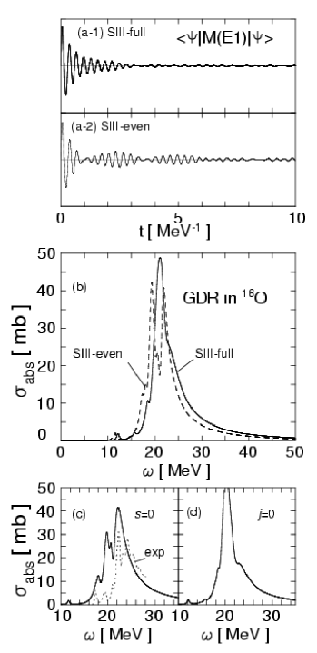
Figure 6: Results of the Skyrme TDHF+ABC for GDR in ¹⁶O. (a-1) Time evolution of the $E1$ moment as a function of time calculated with the SIII-full. (a-2) The same as (a-1) but with SIII-even. (b) Calculated photoabsorption cross section as a function of excitation energy. The SIII-full calculation (solid line) is compared to the SIII-even (dashed line). The smoothing parameter $\Gamma=0.5$ MeV is used. (c) The same as (b) but neglecting the spin density $\mathbf{s}$. Experimental photoneutron cross section ($\times 3.5$) is shown by the dotted line Berman and Fultz (1975). (d) The same as (b) but neglecting the current density $\mathbf{j}$. See text for details.

The continuum RPA with the Skyrme energy functional is a standard method for describing collective excitations in closed-shell spherical nuclei. However, its fully-self-consistent calculations have not been achieved in practice, neglecting residual spin-orbit and Coulomb interactions. In addition, some of the time-odd densities, which are known to be important for nuclear moment of inertia and the local Galilean invariance Dobaczewski and Dudek (1995), are often neglected in the continuum RPA. In this section, we present an application of the small-amplitude TDHF+ABC method to the giant dipole resonance (GDR) in ¹⁶O. Then, we compare the result with that of the former 1D continuum RPA (which neglected the residual spin-orbit, Coulomb, and spin-spin parts), discussing effects of the residual interactions.

We adopt the Skyrme energy functional as same as Eqs. (A.2), (A.15), and (A.16) in Ref. Bonche et al. (1987). The static HF+BCS code based on this functional is called EV8 which assumes the parity and the $z$-signature symmetry. In the present work, we do not assume any symmetry, in order to allow a time-dependent state to be any Slater determinant during the time evolution. The energy density is written in terms of local densities as

$${\cal H}({\mathbf{r}})=\frac{1}{2m}\tau({\mathbf{r}})+{\cal H}^{\rm even}({\mathbf{r}})+{\cal H}^{\rm odd}({\mathbf{r}}),$$ (30)

with

$${\cal H}^{\rm even}({\mathbf{r}}) = {\cal H}^{\rm even}[\rho^{n},\rho\triangle\rho,\rho\tau,\rho\overleftrightarrow{\nabla}\cdot\overleftrightarrow{\mathbf{J}}],$$ (31)

$${\cal H}^{\rm odd}({\mathbf{r}}) = {\cal H}^{\rm odd}[\mathbf{j}^{2},\mathbf{s}^{2},\mathbf{s}\cdot\nabla\times\mathbf{j}].$$ (32)

Here, we follow the notation in Ref. Dobaczewski and Dudek (1995). According to Ref. Bonche et al. (1987), terms of $\mathbf{s}\cdot\mathbf{T}-\overleftrightarrow{\mathbf{J}}^{2}$, $\mathbf{s}\cdot\triangle\mathbf{s}$, and $(\nabla\cdot\mathbf{s})^{2}$ are omitted. The energy functional, ${\cal H}^{\rm even}+{\cal H}^{\rm odd}$, keeps the local gauge invariance Engel et al. (1975); Dobaczewski and Dudek (1995). It is customary in the static HF calculation to take account of the center-of-mass correction by multiplying the first term in Eq. (30) by a factor $(A-1)/A$. We use this correction both for static and dynamic calculations.

In order to see effects of time-odd components, we adopt the SIII interaction which was used in the 1D continuum RPA calculation in Ref. Liu and van Giai (1976). We perform the TDHF calculation with the full functional of ${\cal H}^{\rm even}+{\cal H}^{\rm odd}$, and the one neglecting ${\cal H}^{\rm odd}$. Hereafter, let us call the former functional “SIII-full”, and the latter “SIII-even”. The instantaneous external field is chosen as

$$V_{\rm ext}({\mathbf{r}},t)=\epsilon{\cal M}(E1,\mu=0)\delta(t)=\epsilon e^{(E1)}rY_{10}(\hat{{\mathbf{r}}})\delta(t),$$ (33)

where $e^{(E1)}$ indicates the $E1$ recoil charge, $Ne/A$ for protons and $-Ze/A$ for neutrons. $\epsilon$ is an arbitrary small number. Then, solving the TDHF equation

$$i\frac{\partial}{\partial t}\phi_{i}(t)=\left\{-\frac{1}{2m}\nabla^{2}+V^{\rm even}(t)+V^{\rm odd}(t)\right\}\phi_{i}(t),$$ (34)

for $i=1,\cdots,A$. The time evolution is performed up to $t=30$ MeV^-1. The time-even mean field, $V^{\rm even}$, has been well tested against a large number of experimental observations. In order to test the time-odd mean field, $V^{\rm odd}$, we need to investigate dynamical properties of nuclei.

Figure 6 (a) shows time evolution of calculated $E1$ dipole moment, $\langle{\Psi(t)}|\mathcal{M}(E1)|{\Psi(t)}\rangle$. In the SIII-even calculation, we see a beating pattern which results in two main peaks of the dashed line in Fig. 6 (b). This is in a good agreement with the result of the 1D continuum RPA Liu and van Giai (1976). However, the inclusion of the time-odd mean field, which is necessary for the Galilean invariance, changes the strength distribution into a single peak (solid line). We decompose effects of time-odd densities into those of current density $\mathbf{j}$ and spin density $\mathbf{s}$ in Fig. 6 (c) and (d), respectively. The current density provides additional residual interaction to push the GDR to higher energy by $0.5-1.3$ MeV, while the spin density merges the two main peaks into one. This effect of time-odd density is not special to the SIII interaction. The same effect is observed with the SGII parameters of the Skyrme interaction. See Ref. Nakatsukasa and Yabana (2004b) for a brief report on the same calculation with the SGII force. It is somewhat surprising that not only the current but also the spin density significantly modify the GDR structure. Photoneutron cross section data Berman and Fultz (1975) are shown in the panel (c) by a dotted line. Their absolute values are multiplied by 3.5, since the data indicates less than 20 % of the TRK sum rule. The experimental shape of the GDR resembles that of the SIII-even calculation, but the two main peaks are calculated lower by about 3 MeV. Agreement on the main peak position is slightly improved in the SIII-full calculation, though the calculated peak is still lower than the experiment by $2-2.5$ MeV.

If the interaction commutes with the $E1$ operator, the oscillator sum

$$S(E1) \equiv \int_{0}^{\infty}EB(E1;0^{+}\rightarrow E(1^{-}))dE,$$ (35)

$$= \sum_{\mu=-1}^{1}\int_{0}^{\infty}E\left|\langle{E(1\mu)}|\mathcal{M}(E1,\mu)|{0}\rangle\right|^{2}dE,$$ (36)

is identical to the TRK classical sum rule value

$$S(E1)_{\rm class}=\frac{9e^{2}}{8\pi m}\frac{NZ}{A}.$$ (37)

For ¹⁶O, the classical sum rule gives $S(E1)_{\rm class}=59.4$ e² fm² MeV. Since the Skyrme interaction has momentum and isospin dependence, the classical sum rule is violated to a certain extent. We have $S(E1)=75.1$ e² fm² MeV for SIII-full, and $S(E1)=67.1$ e² fm² MeV for SIII-even. The enhancement of the TRK sum is 26 % for SIII-full and it reduces to 13 % if we neglect the time-odd mean field. This difference mainly comes from the spin density. If we integrate the strength in the energy region up to 30 MeV, we have $S(E1)\approx S(E1)_{\rm class}$ for both SIII-full and SIII-even.

V.2 $E1$ resonances in even-even Be isotopes

Finally, we apply the small-amplitude TDHF+ABC method to $E1$ resonances in beryllium isotopes. Beryllium nuclei have been extensively studied both theoretically and experimentally (see, e.g., Ref. Ikeda et al. (2004) and references therein). ⁸Be is well-known for the $\alpha$-$\alpha$ clustering structure with an elongated prolate shape. Valence neutrons added to ⁸Be are expected to cause variety of structure change in the ground and excited states Seya et al. (1981); Kanada-En’yo et al. (1995); Itagaki et al. (2000). ¹⁰Be has two neutrons in addition to ⁸Be. The $\alpha$-$\alpha$ distance in the ground state is considered to be slightly smaller than that in ⁸Be. ¹²Be is a semi-magic nucleus ($N=8$), however its properties are different from spherical closed-shell nuclei. The measured spectroscopic factors suggest that the last neutron pair is two-thirds in the $sd$ configurations Navin et al. (2000). The neighboring odd nucleus, ¹¹Be, is famous for the parity inversion and for the halo structure in the ground state. The existence of ¹⁴Be at the drip line beyond $N=8$ also indicates weakening of shell closure at $N=8$. Since both $Z=4$ and $N=10$ are the magic numbers at the prolate superdeformed shape, we expect ¹⁴Be to be deformed as large as ⁸Be. A new mode of excitation of significant interest is the soft $E1$ mode near the neutron drip line Hansen and Jonson (1987); Ikeda (1992). Coupling in the continuum between the soft $E1$ mode and the quadrupole deformation is an unsolved problem which can be addressed by the present method to some extent.

We use the Skyrme interaction of the SIII parameters including the time-odd components (SIII-full). The adopted model space is the adaptive grid in Fig. 1 with $R=10$ fm and $\varDelta r=12$ fm. Usually, the static HF calculation is carried out with constraint on the center of mass at the origin. However, in this calculation, we do not impose any condition on the center-of-mass and on the direction of the principal axis. Although this results in heavy computation for the imaginary-time step, it turns out that this is important for the stable time evolution of the TDHF state kicked off by the external perturbation. The external field is the same form as Eq. (33), but includes $rY_{1\pm 1}$. The TDHF calculation with the perturbative $E1$ field provides the $E1$ intrinsic strength, $dB(\omega,{\cal M}(E1,K))/d\omega$ through Eq. (25). Assuming the strong coupling scheme Bohr and Mottelson (1975), the $B(E1)$ transition strength in the laboratory frame is given by

$$\frac{dB(\omega;E1)}{d\omega} \equiv \int dE_{x}\ B(E1;0^{+}\rightarrow E_{x}(1^{-}))\delta(\omega-E_{x}),$$ (38)

$$= \sum_{K}\int dE_{x}|\langle{E_{x}}|{\cal M}(E1,K)|{0}\rangle|^{2}\delta(\omega-E_{x}),$$

$$= \sum_{K=0,\pm 1}\frac{dB(\omega;{\cal M}(E1,K))}{d\omega}.$$

Here, the state $|{0}\rangle$ ($|{E_{x}}\rangle$) is the intrinsic ground (excited) state.

The static HF calculation predicts all these nuclei to be deformed in prolate shape in the ground state. Calculated quadrupole deformations are given in Table 1. As we expected, ⁸Be and ¹⁴Be possess large deformation. ¹²Be has the smallest deformation, but its proton distribution has a moderate deformation. The static HF analysis on Be isotopes with the SIII force have been already done in Ref. Takami et al. (1995). The total binding energies are well reproduced. Calculated occupied single-particle energies are listed in Table 2. In the linear response approximation of the TDHF, the neutron continuum plays its role at energies higher than the absolute value of single-particle energy of the last-occupied neutron. Since the proton orbitals become deeply bound in neutron-rich nuclei, the proton continuum is expected to be less important. However, in these Be isotopes, the protons are important to produce prolate deformation of the mean field.

Table 1: Calculated quadrupole deformation for even-even Be isotopes. The last two columns show deformation of neutron and proton density distribution, $\beta_{n}$ and $\beta_{p}$, separately.

	$\beta$	$\beta_{n}$	$\beta_{p}$
8Be	1.07	1.06	1.09
10Be	0.39	0.33	0.49
12Be	0.12	0.07	0.22
14Be	0.74	0.77	0.66

Table 2: Calculated neutron (n) and proton (p) single-particle energies in units of MeV for Be isotopes. Each state has a two-fold degeneracy associated with the time-reversal symmetry.

8Be		10Be		12Be		14Be
n	p	n	p	n	p	n	p
-24.8	-22.9	-26.3	-31.6	-25.5	-36.7	-24.9	-39.1
-13.3	-11.5	-12.5	-16.0	-11.5	-20.6	-14.0	-25.7
		-9.7		-10.3		-9.1
				-4.3		-3.5
						-2.6

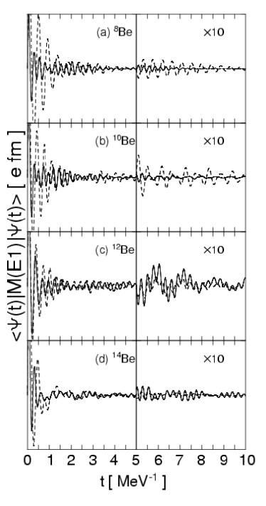
Figure 7: Calculated $E1$ moment as functions of time for (a) ⁸Be, (b) ¹⁰Be, (c) ¹²Be, and (d) ¹⁴Be. The dashed (solid) line indicates the external field with $K=0$ ($K=\pm 1$). Scale of the vertical axis is arbitrary because it linearly depends on the small parameter $\epsilon$. It is magnified by a factor of five for the latter half of period, $5<t<10$ MeV^-1.

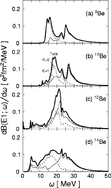
Figure 8: Calculated values of $dB(E1;0\rightarrow 1^{-})/d\omega$ for ^8,10,12,14Be. The smoothing parameter $\Gamma=0.2$ MeV is used. The thin dashed (solid) line is a contribution of $K^{\pi}=0^{-}$ $(1^{-})$ states and the thick solid line for the total strength.

Now let us discuss dynamical properties of these nuclei. In Fig. 7, calculated time-dependent $E1$ moment is presented as functions of time. The time evolution is calculated up to $t=30$ MeV^-1. The beginning third of the total period is shown in Fig. 7. Note that the amplitude is magnified by a factor of 10 in the latter half of period. Performing the Fourier transform, calculated $B(E1)$ transition strength is shown in Fig. 8. In ⁸Be, we observe large splitting of the GDR peak associated with the large quadrupole deformation ($\beta\approx 1$). The magnitude of splitting is more than 10 MeV, that brings down the $K=0$ peak (the oscillation along the symmetry axis) to around 15 MeV in energy. In Fig. 7 (a), the amplitude of the $K=0$ oscillation almost monotonically decays as time increases, while that of the $K=1$ mode shows a beating pattern. This results in a splitting of the high-lying $K=1$ peak. In the total $B(E1)$ strength function, this is seen as a small peak in the middle of two main peaks. We also see that the $K=0$ oscillation stays longer than the $K=1$. This is because the peak position is near the particle decay threshold, thus, the allowed phase space is smaller for the $K=0$ peak (Table 2).

In ¹⁰Be, we see a similar behavior to ⁸Be. Because of the smaller deformation, the lower $K=0$ peak shifts to higher energy by about 5 MeV. Figure 8 (b) again indicates the $K=1$ mode split into two peaks. Although the ground-state deformation in ¹⁰Be is less than half of ⁸Be, the energy splitting between the lowest and highest peaks is still as large as $7\sim 8$ MeV.

Next, let us discuss ¹²Be. The calculated quadrupole deformation is the smallest among these even-even isotopes. In contrast to ^8,10Be, we do not see a distinguished double-peak structure. The GDR shows a peak at $21$ MeV with a broader structure around 25 MeV. There exist low-energy $E1$ strength in the continuum below 10 MeV. The peak very near zero energy is due to small admixture of the translational mode. Because of this mixing, the response function suffers from spurious oscillatory behavior at energy below 2 MeV. Thus, we concentrate our focus on states at $\omega>2$ MeV.

Though the $B(E1)$ strength in low energy looks small compared to that in the main GDR, the integrated strength in the energy region of $2<\omega<10$ MeV amounts to $B(E1)\approx 0.14$ e² fm². The lowest sharp peak at 4.5 MeV has $B(E1;0^{+}\rightarrow 1^{-})\approx 0.023$ e² fm². The next lowest peak at 5.6 MeV has $B(E1)\approx 0.027$ e² fm². Both peaks have a dominant $K=1$ character. The low-lying $1^{-}$ state has been recently observed in ¹²Be Iwasaki et al. (2000). The observed excitation energy is $E_{x}=2.68(3)$ MeV with $B(E1;0^{+}\rightarrow 1^{-})=0.051(13)$ e² fm². Our result is higher in energy by a factor of two and the sum of $B(E1)$ for the lowest two peaks is comparable to the experiment. The two-neutron pairing model in Ref. Bonaccorso and Mau (1997) predicted the $1^{-}$ energy very well (2.7 MeV) but about five times overestimated $B(E1)$. The shell model calculation with extended single-particle wave functions in Ref. Sagawa et al. (2001) well reproduced the lowest $1^{-}$ state ($E_{x}=2.14\sim 2.9$ MeV with $B(E1)=0.063\sim 0.072$ e² fm² depending on the interaction and model space). They also calculated $B(E1)$ strength distribution in the GDR energy region without taking account of the continuum. Although their results strongly depend on the adopted interaction and model space, the calculated GDR energy is lower than ours. A striking difference from our result is that they have predicted three main peaks with the WBP interaction. It is not clear at present whether this difference is due to the treatment of the continuum or to the ground-state correlation.

Finally, let us move to the drip line, ¹⁴Be. The doubly-magic closed-shell configuration ($N=10$, $Z=4$) at superdeformation leads to the large quadrupole deformation of $\beta=0.74$. The $K=0$ and $K=1$ resonance peaks are at different positions whose centroids are at 15 MeV and 24 MeV. Figure 7 (d) indicates quick damping of the $K=0$ oscillation. The oscillating pattern almost disappears by $t=3$ MeV^-1. This leads to the large width of the $K=0$ peak in Fig. 8 (d). As a consequence of the large width, the double-peak structure in the total $B(E1)$ strength function is not as clear as in ^8,10Be. It looks more like a single broad resonance at 20 MeV with the width of about 20 MeV. In Fig. 7 (d), after the $K=0$ mode disappears, the $K=1$ mode becomes dominant at $t>3$ MeV^-1. This long-lived high-frequency $K=1$ mode results in sub-peaks embedded in the broad $K=1$ resonance ($20<\omega<25$ MeV).

It is known that the weakly bound neutrons strongly couples to the continuum and produces the large dipole strength Blatt and Weisskopf (1952). The Coulomb breakup of ¹¹Be is a typical example Nakamura et al. (1994). This is often called “threshold effect” which has a peak at the threshold energy. Since the SIII interaction gives the last neutron binding of $2-3$ MeV, the threshold effect is weak. In the present calculation, we do not have significant threshold strength. On the other hand, another soft dipole peak is seen at 5 MeV. This peak carries $B(E1)\approx 0.26$ e² fm². A Coulomb dissociation experiment seems to suggest enhanced strength at $E_{x}\approx 2$ and 5 MeV Labiche et al. (2001). The shell-model calculation of Ref. Sagawa et al. (2001) also indicates a similar peak ($E_{x}=6.76\sim 7.46$ MeV with $B(E1)=0.097\sim 0.146$ e² fm²). Using the SGII interaction, this peak is at 7 MeV with $B(E1)\approx 0.14$ e² fm² Nakatsukasa et al. (2004), which well agrees with the shell-model result. On the GDR main peaks, our result looks rather different from the shell-model: the shell-model indicates a single main peak at $12-17$ MeV, while we have a broad resonance whose centroid is around 20 MeV. Since the shell model also indicates continuous $E1$ strength in the energy region of $\omega>10$ MeV, this difference may be simply due to lack of the continuum in Ref. Sagawa et al. (2001).

Calculated TRK sum rule values are listed in Table 3. The enhancement is slightly smaller than the spherical ¹⁶O case. Among the even-even Be isotopes, the enhancement is the biggest for ¹²Be whose deformation is the smallest. According to the analysis on ¹⁶O in Sec. IV.1, about the half of this enhancement comes form effect of the time-odd spin density. The large deformation leads to a strong coupling to the $K$-quantum number, and this may restrict dynamics of spin degrees of freedom. The soft $E1$ strength, which is defined by the oscillator sum up to 15 MeV in the table, varies among these isotopes. The large value in ⁸Be is due to the large ground-state deformation that brings the low-energy $K=0$ peak down close to 14 MeV. In ¹⁴Be, it is the largest. This is due to combination of the deformation, the soft dipole peak at 5 MeV, and the large width of the $K=0$ resonance at 15 MeV. The deformation parameter $\delta$ is estimated from the average energies of $K=0$ and $K=1$ modes. We use Eq. (6-344) in Ref. Bohr and Mottelson (1975). The $\delta$ turns out to be much smaller than the deformation of the HF density distribution, $\beta$. The deformation derived from the GDR splitting is known to well agree with that from the $E2$ moment for actinide nuclei Bohr and Mottelson (1975). In light nuclei, the geometrical interpretation of the GDR frequencies may not be justified so well.

Table 3: Energy weighted sum rule values in units of e² fm² MeV. The second column shows values of the classical TRK formula. The small-amplitude TDHF+ABC calculation produces values in the third columns. The fourth column gives the soft $E1$ strength of the energy weighted sum, which is defined by $\omega<15$ MeV. The last column indicates the deformation parameter obtained by the splitting of the GDR peaks.

	$S(E1)_{\rm class}$	$S(E1)$	$S(E1;E<15\mbox{MeV})$	$\delta$
8Be	$29.7$	$34.0$	$3.14$	$0.43$
10Be	$35.7$	$42.8$	$1.26$	$0.21$
12Be	$39.6$	$48.2$	$2.54$	$0.05$
14Be	$42.5$	$52.2$	$7.57$	$0.35$

VI Conclusion

We have developed the linear response theory in the continuum applicable to deformed systems. The exact treatment of the continuum is done by the iterative method for construction of the Green’s function in the 3D Cartesian grid space (3D continuum RPA). The method is identical to the conventional 1D continuum RPA in the spherical limit. At the same time, we have shown that the approximate but yet accurate treatment of the continuum can be done by the absorbing boundary condition (ABC) approach. The small-amplitude TDHF+ABC method in the linear response regime is practically identical to the 3D continuum RPA. Applications of these methods to the TDHF with the BKN interaction reveals their usefulness and accuracy. The real-time TDHF method has a difficulty when we study excitation modes coupled to the zero modes. Since the method is fully self-consistent, the increase of model space (finer grid spacing) will solve the problem, though it requires heavier computation.

Applications to systems with a realistic effective interaction have been performed with the small-amplitude Skyrme TDHF+ABC. The analysis on the GDR in ¹⁶O suggests a significant contribution coming from the time-odd mean field which was often neglected in the 1D continuum RPA. The peak structure in the continuum is affected by these residual interactions, especially by the spin density. Since the spin-dependent terms in the Skyrme energy functional, such as $\mathbf{s}^{2}$, $\mathbf{s}\cdot\triangle\mathbf{s}$, and $(\nabla\cdot\mathbf{s})^{2}$, are not linked to the time-even components by the local gauge invariance, the analysis may give a useful constraint on these parts of the Skyrme functional.

The coupling to the continuum becomes more important for weakly bound systems. We have studied the deformed continuum of the GDR in Be isotopes. The large deformation splitting of about 10 MeV is predicted for ^8,14Be. The $K=0$ main peak is significantly lowered by the deformation to less than 15 MeV. The time evolution of the $E1$ moment indicates different damping between ⁸Be and neutron-rich Be isotopes, especially for the $K=0$ dipole mode. The soft dipole strength ($E<10$ MeV) appears in ¹²Be and ¹⁴Be. Considering the fact that the SIII parameters were not determined by the isovector properties, we have a reasonable agreement with experiment on the low-energy $1^{-}$ state in ¹²Be and ¹⁴Be.

In this paper, we have studied only the IV GDR in neutron-rich nuclei, because of the numerical difficulty discussed above. The IS modes in neutron-rich deformed nuclei are also interesting to investigate. For instance, the octupole correlation in superdeformed ¹⁴Be is expected to be stronger than ⁸Be. This is because the superdeformed magic numbers are classified into two category, and the $N=10$ shell closure has a stronger octupole correlation than the $N=4$ Nazarewicz and Dobaczewski (1992); Nakatsukasa et al. (1992). The small-amplitude TDHF+ABC may be a good method to see how the continuum affects this expectation,

An important extension of the present approaches is the inclusion of pairing. Since the pairing plays an important role in heavy nuclei, this is very desirable but a difficult task. In this respect, we should mention that the HFB-based continuum QRPA has been recently proposed by Matsuo Masuo (2001) to take account of the continuum for both particle-hole (p-h) and particle-particle (p-p)/hole-hole (h-h) channels. The combination of the 3D continuum RPA and the continuum QRPA may produce a general theory to calculate excited states in the p-h, p-p, and h-h continuum for nuclei in the whole nuclear chart.