Quantum Monte Carlo calculations of excited states in $A=6-8$ nuclei

Abstract

A variational Monte Carlo method is used to generate sets of orthogonal trial functions, $\Psi_{T}(J^{\pi},T)$, for given quantum numbers in various light p-shell nuclei. These $\Psi_{T}$ are then used as input to Green’s function Monte Carlo calculations of first, second, and higher excited $(J^{\pi},T)$ states. Realistic two- and three-nucleon interactions are used. We find that if the physical excited state is reasonably narrow, the GFMC energy converges to a stable result. With the combined Argonne v₁₈ two-nucleon and Illinois-2 three-nucleon interactions, the results for many second and higher states in $A$ = 6–8 nuclei are close to the experimental values.

I Introduction

Quantum Monte Carlo methods have proved to be very accurate and powerful tools for studying the structure of light nuclei with realistic two- and three-nucleon interactions. In a series of papers, we have calculated about 40 ground and low-lying excited state energies of different $(J^{\pi},T)$ quantum numbers in $A$ = 6–10 nuclei with an accuracy of $\sim$ 1–2% PPCW95 ; PPCPW97 ; WPCP00 ; PPWC01 ; PVW02 . The first step is a variational Monte Carlo (VMC) calculation to find an optimal trial function, $\Psi_{T}(J^{\pi},T)$ for a given state. The $\Psi_{T}$, which is antisymmetric by explicit construction, is then used as input to a Green’s function Monte Carlo (GFMC) algorithm, which projects out the lowest-energy eigenstate by a propagation in imaginary time, $\tau$. The algorithm preserves the quantum numbers of $\Psi_{T}$, although it may introduce symmetric noise into the propagated $\Psi(\tau)$. In principle, $\Psi(\tau)$ for large $\tau$ approaches the exact lowest-energy eigenstate with the specified quantum numbers.

VMC calculations of second and higher excited $(J^{\pi},T)$ states have also been made, because a major step in the preparation of an optimal $\Psi_{T}$ is a diagonalization in the small single-particle basis of different possible spatial-symmetry states PPCPW97 ; WPCP00 ; PVW02 . GFMC calculations of second or higher $(J^{\pi},T)$ states have not been attempted previously in nuclear physics, under the expectation that any small contamination of the excited trial state by the true first state would drive the calculated energy below its proper value. However, as is described in this paper, we have found that it is possible to obtain useful GFMC predictions of multiple states with the same quantum numbers.

In this paper we report such GFMC calculations of second and higher $(J^{\pi},T)$ states in light ($A$ = 6–8) p-shell nuclei. VMC calculations of these states were reported previously PPCPW97 ; WPCP00 , but we have made significant improvements in the trial functions since then. Details of the recent VMC work are discussed in Sec. II. For the GFMC calculations, we find that the propagated energy, $E(\tau)$, for many states is stable and a useful excitation energy can be extracted. GFMC calculations for ground states are reviewed in Sec. III, where we also describe an improved algorithm for propagation with three-nucleon interactions that is both faster and more accurate than what we had used previously. The GFMC algorithm for higher excited states is described in Sec. IV, along with various orthogonality tests. Numerical results are given in Sec. V for the Argonne v₁₈ (AV18) and simplified v${}_{8^{\prime}}$ (AV8^′) two-nucleon ($N\!N$) interactions WSS95 , and for AV18 with either the Urbana IX (UIX) or Illinois-2 (IL2) three-nucleon ($N\!N\!N$) interactions PPCW95 ; PPWC01 added. We find, consistent with our studies of first $(J^{\pi},T)$ states, that the AV18/IL2 Hamiltonian gives a good representation of the experimental spectrum; the RMS deviation from 36 experimental energies with $6\leq A\leq 8$ is only 0.60 MeV. Some concluding remarks are given in Sec. VI.

II VMC trial functions

The VMC trial function, $\Psi_{T}(J^{\pi};T)$, for a given nucleus, is constructed from products of two- and three-body correlation operators acting on an antisymmetric single-particle state with the appropriate quantum numbers. The correlation operators reflect the influence of the interactions at short distances, while appropriate boundary conditions are imposed at long range. The $\Psi_{T}$ contains variational parameters that are adjusted to minimize the energy expectation value, $E_{T}=\langle\Psi_{T}|H|\Psi_{T}\rangle/\langle\Psi_{T}|\Psi_{T}\rangle$, which is evaluated by Metropolis Monte Carlo integration.

A good variational trial function has the form

$$|\Psi_{T}\rangle=\left[1+\sum_{i<j<k}U^{TNI}_{ijk}\right]\left[{\mathcal{S}}\prod_{i<j}(1+U_{ij})\right]|\Psi_{J}\rangle\ .$$ (1)

The $U_{ij}$ and $U^{TNI}_{ijk}$ are non-commuting two- and three-nucleon correlation operators, ${\mathcal{S}}$ indicates a symmetric sum over all possible orderings, and $\Psi_{J}$ is the fully antisymmetric Jastrow wave function. For s-shell nuclei the latter has the simple form

$$|\Psi_{J}\rangle=\left[\prod_{i<j<k}f^{c}_{ijk}\right]\left[\prod_{i<j}f_{c}(r_{ij})\right]|\Phi_{A}(JMTT_{3})\rangle\ .$$ (2)

Here $f_{c}(r_{ij})$ and $f^{c}_{ijk}$ are central two- and three-body correlation functions and $\Phi_{A}$ is a Slater determinant in spin-isospin space, e.g., for the $\alpha$-particle, $|\Phi_{4}(0000)\rangle={\mathcal{A}}|p\uparrow p\downarrow n\uparrow n\downarrow\rangle$.

The correlation operator $U_{ij}$ includes spin, isospin, and tensor terms:

$$U_{ij}=\sum_{p=2,6}u_{p}(r_{ij})O^{p}_{ij}\ ,$$ (3)

where the $O^{p=1,6}_{ij}=[1,{\bf\sigma}_{i}\cdot{\bf\sigma}_{j},S_{ij}]\otimes[1,{\bf\tau}_{i}\cdot{\bf\tau}_{j}]$ are the same static operators that appear in the $N\!N$ potential. The functions $f_{c}(r)$ and $u_{p}(r)$ are generated by solving a set of six coupled differential equations with embedded variational parameters W91 : two single-channel equations in ¹S and ¹P waves, and two coupled-channel equations in ³S and ³P waves. The $U^{TNI}_{ijk}$ has the spin-isospin structure of the dominant parts of the $N\!N\!N$ interaction as suggested by perturbation theory.

For p-shell nuclei, the Jastrow wave function, $\Psi_{J}$, is necessarily more complicated. It starts with a sum over independent-particle terms, $\Phi_{A}$, that have 4 nucleons in an $\alpha$-like core and $(A-4)$ nucleons in p-shell orbitals. We use $LS$ coupling to obtain the desired $JM$ value of a given state, as suggested by standard shell-model studies CK65 . We also need to specify the spatial symmetry $[n]$ of the angular momentum coupling of the p-shell nucleons BM69 . Different possible $LS[n]$ combinations lead to multiple components in the Jastrow wave function. This independent-particle basis is again acted on by products of central pair and triplet correlation functions, but now they depend upon the shells (s or p) occupied by the particles and on the $LS[n]$ coupling:

$$|\Psi_{J}\rangle = {\mathcal{A}}\left\{\Big{[}\prod_{i<j<k}f^{c}_{ijk}\Big{]}\Big{[}\prod_{i<j\leq 4}f_{ss}(r_{ij})\Big{]}\sum_{LS[n]}\Big{(}\beta_{LS[n]}\Big{[}\prod_{k\leq 4<l\leq A}f^{LS[n]}_{sp}(r_{kl})\Big{]}\right.$$ (4)

$$\times \left.\Big{[}\prod_{4<l<m\leq A}f^{LS[n]}_{pp}(r_{lm})\Big{]}|\Phi_{A}(LS[n]JMTT_{3})_{1234:5\ldots A}\rangle\Big{)}\right\}\ .$$

The operator ${\mathcal{A}}$ indicates an antisymmetric sum over all possible partitions of the $A$ particles into 4 s-shell and $(A-4)$ p-shell ones. The pair correlation for both particles within the s-shell, $f_{ss}$, is similar to the $f_{c}$ of the $\alpha$-particle. The pair correlations for both particles in the p-shell, $f^{LS[n]}_{pp}$, and for mixed pairs, $f^{LS[n]}_{sp}$, are similar to $f_{ss}$ at short distance, but their long-range structure is adjusted to give appropriate clustering behavior, and they may vary with $LS[n]$.

The single-particle wave functions $\Phi_{A}$ are given by:

$$|\Phi_{A}(LS[n]JMTT_{3})_{1234:5\ldots A}\rangle = |\Phi_{4}(0000)_{1234}\Big{[}\prod_{4<l\leq A}\phi^{LS[n]}_{p}(R_{\alpha l})\Big{]}$$

$$\times \left\{\Big{[}\prod_{4<l\leq A}Y_{1m_{l}}(\Omega_{\alpha l})\Big{]}_{LM_{L}[n]}\Big{[}\prod_{4<l\leq A}\chi_{l}(\frac{1}{2}m_{s})\Big{]}_{SM_{S}}\right\}_{JM}\Big{[}\prod_{4<l\leq A}\nu_{l}(\frac{1}{2}t_{3})\Big{]}_{TT_{3}}\rangle\ .$$

The $\phi^{LS[n]}_{p}(R_{\alpha l})$ are p-wave solutions of a particle in an effective $\alpha-N$ potential that has Woods-Saxon and Coulomb parts. They are functions of the distance between the center of mass of the $\alpha$ core and nucleon $l$, and may vary with $LS[n]$. The depth, width, and surface thickness of the single-particle potential are additional variational parameters of the trial function. The overall wave function is translationally invariant, so there is no spurious center of mass motion.

The $\beta_{LS[n]}$ mixing parameters of Eq. (4) are determined by a diagonalization procedure, in which matrix elements

$$E_{T,ij} = \langle\Psi_{T}(\beta_{i})|H|\Psi_{T}(\beta_{j})\rangle\ ,$$ (6)

$$N_{T,ij} = \langle\Psi_{T}(\beta_{i})|\Psi_{T}(\beta_{j})\rangle\ ,$$ (7)

are evaluated using trial functions $\Psi_{T}(\beta_{i})\equiv\Psi_{T}(\beta_{i}=1,\beta_{j\neq i}=0)$. Although the $\Phi_{A}(LS[n]JMTT_{3})$ are orthogonal due to spatial symmetry, the pair and triplet correlations in $\Psi_{T}$ make the different $LS[n]$ components nonorthogonal, so a generalized eigenvalue routine is necessary to carry out the diagonalization.

Table 1: $\beta_{LS[n]}$ components for ⁶He states, listed in order of increasing excitation. (L = S or D as appropriate.)

$(J^{\pi};T)$	1L[2]	3P[11]
$(0^{+};1)$	0.974	-0.228
$(2^{+};1)$	0.922	0.386
$(2^{+};1)$	-0.388	0.922
$(1^{+};1)$		1.
$(0^{+};1)$	0.232	0.973

Table 2: $\beta_{LS[n]}$ components in ⁶Li states, listed in order of increasing excitation.

$(J^{\pi};T)$	3S[2]	3D[2]	1P[11]
$(1^{+},0)$	0.986	0.138	0.098
$(3^{+};0)$		1.
$(2^{+};0)$		1.
$(1^{+},0)$	-0.109	0.964	-0.242
$(1^{+},0)$	-0.134	0.231	0.964

Table 3: $\beta_{LS[n]}$ components for ⁷He states, listed in order of increasing excitation.

$(J^{\pi};T)$	2P[21]	2D[21]	4S[111]
$(\frac{3}{2}^{-},\frac{3}{2})$	0.837	0.515	-0.182
$(\frac{1}{2}^{-},\frac{3}{2})$	1.
$(\frac{5}{2}^{-},\frac{3}{2})$		1.
$(\frac{3}{2}^{-},\frac{3}{2})$	-0.392	0.805	0.445
$(\frac{3}{2}^{-},\frac{3}{2})$	0.373	-0.317	0.872

Table 4: $\beta_{LS[n]}$ components for ⁷Li states, listed in order of increasing excitation. (L = P or F as appropriate.)

$(J^{\pi};T)$	2L[3]	4P[21]	4D[21]	2P[21]	2D[21]	2S[111]
$(\frac{3}{2}^{-},\frac{1}{2})$	0.995	0.086	0.026	0.005	-0.050
$(\frac{1}{2}^{-},\frac{1}{2})$	0.988	-0.003	-0.098	-0.116		-0.024
$(\frac{7}{2}^{-},\frac{1}{2})$	0.990		0.138
$(\frac{5}{2}^{-},\frac{1}{2})$	0.988	0.114	0.072		-0.079
$(\frac{5}{2}^{-},\frac{1}{2})$	-0.079	0.957	-0.058		0.274
$(\frac{3}{2}^{-},\frac{1}{2})$	-0.084	0.952	0.250	-0.087	0.132
$(\frac{1}{2}^{-},\frac{1}{2})$	0.049	0.841	-0.111	0.523		-0.069
$(\frac{7}{2}^{-},\frac{1}{2})$	-0.129		0.992
$(\frac{5}{2}^{-},\frac{1}{2})$	-0.088	-0.009	0.968		0.235
$(\frac{5}{2}^{-},\frac{1}{2})$	0.137	-0.263	-0.224		0.928

Table 5: $\beta_{LS[n]}$ components for ⁸He states, listed in order of increasing excitation. (L = S or D as appropriate.)

$(J^{\pi};T)$	1L[22]	3P[211]
$(0^{+};2)$	0.794	-0.608
$(2^{+};2)$	0.928	-0.373
$(1^{+};2)$		1.
$(0^{+};2)$	0.610	0.792
$(2^{+};2)$	0.377	0.926

Table 6: $\beta_{LS[n]}$ components for ⁸Li states, listed in order of increasing excitation. (L = P, D or F as appropriate.)

$(J^{\pi};T)$	3P[31]	3D[31]	3F[31]	1L[31]	3S[22]	3D[22]	5P[211]	3P[211]	1P[211]
$(2^{+};1)$	0.948	-0.248	-0.094	0.122		-0.116	0.047	0.019
$(1^{+};1)$	0.772	-0.299		0.524	-0.091	-0.074	0.120	-0.112	-0.005
$(3^{+};1)$		0.947	0.126	-0.257		-0.061	-0.135
$(0^{+};1)$	0.995							-0.100
$(1^{+};1)$	-0.588	-0.302		0.733	0.123	0.089	-0.025	-0.031	-0.009
$(2^{+};1)$	0.281	0.908	0.297	-0.038		0.040	-0.056	0.057
$(2^{+};1)$	-0.079	-0.128	0.533	0.823		-0.092	-0.053	0.063
$(1^{+};1)$	0.051	0.873		0.412	-0.221	0.065	-0.045	-0.064	0.078
$(3^{+};1)$		-0.153	0.945	-0.125		-0.229	0.126
$(4^{+};1)$			1.

Table 7: $\beta_{LS[n]}$ components for ⁸Be states, listed in order of increasing excitation. (L = S, D or G as appropriate.)

$(J^{\pi};T)$	1L[4]	3P[31]	3D[31]	3F[31]	5S[22]	5D[22]	1L[22]	3P[211]
$(0^{+};0)$	0.998	-0.055				-0.034	0.016	0.015
$(2^{+};0)$	0.998	0.026	0.041	-0.020	0.002	0.029	0.007	0.008
$(4^{+};0)$	0.999			0.052		-0.015
$(2^{+};0)$	-0.011	0.931	-0.169	0.087	0.284	-0.062	-0.101	-0.055
$(1^{+};0)$		0.957	0.237			-0.165		0.018
$(1^{+};0)$		-0.249	0.959			0.098		0.097
$(3^{+};0)$			0.936	0.287		0.207
$(4^{+};0)$	-0.018			0.691		0.723
$(2^{+};0)$	-0.038	-0.006	0.825	0.230	0.499	0.050	0.111	0.039
$(0^{+};0)$	0.029	0.926				-0.311	0.181	-0.105
$(3^{+};0)$			-0.127	0.782		-0.610
$(2^{+};0)$	0.016	-0.301	-0.376	-0.257	0.782	0.148	-0.011	-0.261

The results for the $\beta_{LS[n]}$ coefficients are shown in Tables 1–7. Tables 1, 2, 3, and 5 show the complete set of possible p-shell states for ⁶He, ⁶Li, ⁷He, and ⁸He, respectively. Tables 4, 6, and 7 show the lowest-lying p-shell states for ⁷Li, ⁸Li, and ⁸Be. In previous work WPCP00 , only the two most spatially symmetric $LS[n]$ components were included in ⁸Li and ⁸Be, but now all are included. The added components have little effect on the energies of the lowest states of given $(J^{\pi},T)$, but their inclusion can be important for higher excited states; they are also expected to be important for some electroweak transitions. The diagonalizations were done for the AV18/UIX Hamiltonian and the resulting $\beta_{LS[n]}$ used for all the Hamiltonians reported here; a few tests have shown insignificant dependence of the $\beta_{LS[n]}$ on $V_{ijk}$.

Additional improvements in the trial wave have been made by refining the detailed shapes of the $u_{p}(r)$, $f_{sp}(r)$, and $f_{pp}(r)$ functions; these improvements are described in more detail with the numerical results in Sec.V.

III GFMC methods for ground states

Green’s function Monte Carlo calculations of light nuclei have previously been performed for ground states of light nuclei PPCW95 ; PPCPW97 ; WPCP00 ; PPWC01 ; PVW02 and for the lowest-energy states with distinct quantum numbers. In this section we briefly review the GFMC method as applied to light nuclei; Refs. PPCPW97 ; WPCP00 ; PVW02 should be consulted for detailed descriptions of the method and tests of its reliability. We then report new algorithmic developments which significantly increase the speed of these calculations. These improvements result in a much more efficient treatment of $N\!N\!N$ interactions, particularly the very small, but computationally expensive, terms when three nucleons are well separated. In the next section we discuss the extensions required to treat excited states of the same quantum numbers.

Starting with the trial function $\Psi_{T}$, GFMC provides a means of computing a wave function propagated in imaginary time:

$$\Psi(\tau)=\exp[-(H-E_{0})\tau]\Psi_{T}\ =\ \exp[-(H-E_{0})\Delta\tau]^{n}\Psi_{T},$$ (8)

by stringing together a series of small time ( $\Delta\tau=\tau/N$) evolution operators. The energy, $E(\tau)$, is evaluated using a “mixed” expectation value between $\Psi_{T}$ and $\Psi(\tau)$:

$$E(\tau)=\langle H(\tau)\rangle_{\rm Mixed}=\frac{\langle\Psi(\tau)|H|\Psi_{T}\rangle}{\langle\Psi(\tau)|\Psi_{T}\rangle}\ .$$ (9)

In principle, $E(\tau)$ is an upper bound to the energy of the lowest eigenstate that is not orthogonal to $\Psi_{T}$.

The $\Psi(\tau)$ is represented by a vector function of ${\bf R}$, where the components of the vector are the amplitudes of each of the distinct spin-isospin states in the system. The propagator

$$G_{\alpha,\beta}({\bf R},{\bf R^{\prime}};\Delta\tau)=\langle{\bf R},\alpha|\exp[-(H-E_{0})\Delta\tau]|{\bf R^{\prime}},\beta\rangle$$ (10)

depends upon the 6A spatial coordinates ${\bf R}$ and ${\bf R^{\prime}}$, as well as the spin-isospin states $\alpha$ and $\beta$. It is calculated with leading errors of $(\Delta\tau)^{3}$. The full wave function is then obtained as a product over many small time steps:

$$\Psi({\bf R}_{n},\tau) = \int G({\bf R}_{n},{\bf R}_{n-1})\cdots G({\bf R}_{1},{\bf R}_{0})$$ (11)

$$\times \Psi_{T}({\bf R}_{0})d{\bf R}_{n-1}\cdots d{\bf R}_{0},$$

where we have omitted the spin-isospin labels for simplicity.

A central ingredient in a GFMC calculation is the propagator $G({\bf R},{\bf R^{\prime}};\Delta\tau)$. It is desirable to use as large a time step $\Delta\tau$ as possible to speed up the calculation, however the maximum time step is limited by the accuracy with which we can evaluate the propagator $G({\bf R},{\bf R^{\prime}};\Delta\tau)$. The short-time propagator typically used for $N\!N$ interactions is

$$G_{\alpha,\beta}({\bf R},{\bf R^{\prime}};\Delta\tau)=$$

$$G_{0}({\bf R},{\bf R^{\prime}})\langle\alpha|\left[{\cal S}\prod_{i<j}\frac{g_{ij}({\bf r}_{ij},{\bf r^{\prime}}_{ij})}{g_{0,ij}({\bf r}_{ij},{\bf r^{\prime}}_{ij})}\right]|\beta\rangle,$$ (12)

where the free-particle propagator $G_{0}$ and the free two-nucleon propagator $g_{0,ij}$ are simple Gaussians PPCW95 , and the interacting pair propagator,

$$g_{ij}({\bf r}_{ij},{\bf r^{\prime}}_{ij};\Delta\tau)=\langle{\bf r}_{ij}|\exp[-\Delta\tau(T_{ij}+v_{ij})]|{\bf r}^{\prime}_{ij}\rangle,$$ (13)

is easily calculable from the two-body potential $v_{ij}$ and the relative kinetic energy $T_{ij}$. We calculate the propagator with the simplified AV8’ interaction, the difference between the full Hamiltonian H and the simplified H’ is treated perturbatively. PPCPW97

Because of the large number of spin-isospin amplitudes which must be evaluated, the overall speed of the computation for larger nuclei is dominated by the calculation of the $N\!N\!N$ propagator. This term was originally treated in a very straightforward manner. Including $N\!N\!N$ interactions, the full propagator $G$ can be calculated as:

$$G_{\alpha,\beta}({\bf R},{\bf R^{\prime}};\Delta\tau) = \exp[E_{0}\tau]\ G_{0}({\bf R},{\bf R^{\prime}})\ \exp[-\sum(V_{ijk}^{R}({\bf R})+V_{ijk}^{R}({\bf R^{\prime}}))\frac{\Delta\tau}{2}]$$ (14)

$$\times \langle\alpha|I_{3}({\bf R};\frac{\Delta\tau}{2})|\gamma\rangle\langle\gamma|\left[{\cal S}\prod_{i<j}\frac{g_{ij}({\bf r}_{ij},{\bf r}^{\prime}_{ij})}{g_{0,ij}({\bf r}_{ij},{\bf r}^{\prime}_{ij})}\right]|\delta\rangle\langle\delta|I_{3}({\bf R^{\prime}};\frac{\Delta\tau}{2})|\beta\rangle,$$

where

$$I_{3}({\bf R};\Delta\tau/2)=\left[1-\frac{\Delta\tau}{2}\sum V_{ijk}^{\pi}({\bf R})\right].$$ (15)

Here $V_{ijk}^{R}$ is the spin-isospin independent part of the $N\!N\!N$ interaction, which can be trivially exponentiated. The $V_{ijk}^{\pi}$ contains the two-pion-exchange component of the $N\!N\!N$ interaction, and in the case of the Illinois potentials, the three-pion-exchange component.

We have previously employed the fact that the largest part of $V_{ijk}^{\pi}$ is a sum of products of spin and isospin anticommutators that can be expressed as a sum of terms each of which contain only two-nucleon spin and isospin operators. This part, which we denote $\tilde{V}_{ijk}$, is not much more difficult to treat than the typical $N\!N$ potential, i.e., while it involves spatial coordinates of three particles, the spin-isospin algebra is equivalent to that of an $N\!N$ interaction.

The remaining terms depend upon the spins and isospins of three nucleons and are comparatively weak. If we define a propagator $\tilde{G}$ which is obtained from the $N\!N$ potential $v_{ij}$ and the $\tilde{V}_{ijk}$ through Eq. (14), the complete propagator including the full $N\!N\!N$ interaction can be written as:

$$G_{\alpha,\beta}({\bf R}_{M},{\bf R}_{1};M\Delta\tau) = [1-(V_{ijk}({\bf R}_{M})-\tilde{V}_{ijk}({\bf R}_{M}))M\frac{\Delta\tau}{2}]$$ (16)

$$\times \left[\prod\tilde{G}({\bf R}_{M},{\bf R}_{M-1};\Delta\tau)...\tilde{G}({\bf R}_{2},{\bf R}_{1};\Delta\tau)\right][1-(V_{ijk}({\bf R}_{1})-\tilde{V}_{ijk}({\bf R}_{1}))M\frac{\Delta\tau}{2}],$$

where the number $M$ of intermediate steps with the simplified propagator $\tilde{G}$ is typically four to five. This treatment is equivalent to evaluating the propagation with a simplified Hamiltonian containing only two-body spin and isospin operators, and then correcting the end points for the difference between the full $N\!N\!N$ interaction and the simplified one. Clearly this method has the same short-time limit as the original implementation, but the computational time is significantly decreased because the number of full three-nucleon spin-isospin operations is much reduced.

Further generalizing this method, it is possible to introduce artificial fluctuations into the propagator which average to the correct propagator in the short-time limit, but are much more efficient computationally. We can replace the factor $I_{3}({\bf R})$ above (Eq. 15) by

$$I_{3}({\bf R}) = 1-\frac{\Delta\tau}{2}$$ (17)

$$\times \sum_{i<j<k}\int^{1}_{0}dq_{ijk}\ \theta(P_{ijk}-q_{ijk})\ \frac{V_{ijk}}{P_{ijk}},$$

where $\theta(x<0)=0$ and $\theta(x>0)=1$. The function $P_{ijk}$ is an arbitrary function of the particle coordinates $({\bf r}_{i},{\bf r}_{j},{\bf r}_{k})$ subject to the condition $0\leq P_{ijk}\leq 1$. Integrating over the “auxiliary fields” $q_{ijk}$ trivially recovers the original term in the propagator, as with probability $P_{ijk}$ the triplet term is $V_{ijk}/P_{ijk}$ and with probability $1-P_{ijk}$ the triplet contribution is zero. The original formulation for the propagator, Eq. (15), is equivalent to choosing $P_{ijk}=1$.

Choosing a $P_{ijk}$ which decreases as the three-nucleon separation increases is computationally very advantageous, however. Based upon various trials, we have used

$$P_{ijk} = \left\{\begin{array}[]{cl}1,&X_{\mbox{max}}<X_{ijk},\\ X_{ijk}/X_{\mbox{max}},&X_{\mbox{min}}\leq X_{ijk}\leq X_{\mbox{max}},\\ X_{\mbox{min}},&X_{ijk}<X_{\mbox{min}},\end{array}\right.$$ (21)

where

$$X_{ijk}=\tilde{T}(r_{ij})\tilde{T}(r_{ik})+\tilde{T}(r_{ij})\tilde{T}(r_{jk})+\tilde{T}(r_{ik})\tilde{T}(r_{jk}),$$ (22)

$$\tilde{T}(r)=\left\{\begin{array}[]{cl}T(m_{\pi}r),&r>r_{\mbox{max}},\\ T(m_{\pi}r_{\mbox{max}}),&r\leq r_{\mbox{max}}.\end{array}\right.$$ (23)

Here $T(x)$ is the radial tensor function used in $V_{ijk}$ (see Eqs. (3.5-8) of Ref. PPWC01 ) and $r_{\mbox{max}}$ is the location of the maximum of $T(m_{\pi}r)$. For small triplet separations, as effectively specified by $X_{\mbox{max}}$, the full contribution is always calculated. For larger separations, the contribution is calculated less often. Because of the $1/P_{ijk}$ in Eq. (17), one does not want $P_{ijk}$ to become too small; $X_{\mbox{min}}$ is used to control this. Typical values are $X_{\mbox{max}}=5.0$ and $X_{\mbox{min}}=0.01~{}$.

This technique essentially invokes a larger time step for well-separated triplets. Tests are of course required to make sure that the overall time step is small enough to avoid physically significant errors in the expectation values of interest. This method is particularly important in nuclear physics applications, where the triplet computations are so expensive, but could also be employed in other systems where quantum Monte Carlo methods are used.

We have also adopted a similar scheme in computing the quadratic spin-orbit $(L\cdot S)^{2}$ and angular momentum ($L^{2}$) contributions to the energy in both VMC and GFMC calculations. These terms in the interaction are typically quite small at large pair separations, and so we can evaluate them with a probability $P_{ij}$ and then multiply the calculated contribution with the inverse of $P_{ij}$. Using this scheme enables one to calculate the energies and expectation values in the AV18 interaction at a computational cost much closer to evaluating the simplified AV8^′ interaction.

IV GFMC evaluation of excited states

It is possible to treat at least a few excited states with the same quantum numbers using VMC and GFMC methods. The VMC calculations have been described above, and essentially involve solving a generalized eigenvalue problem, Eqs. (6) and (7). The same basic method can be applied in GFMC calculations, though the implementation is slightly more involved. In this section, $\Psi_{T,i}$ represents the trial wave function for the $i^{th}$ state of specified $(J^{\pi},T)$ and $\Psi_{i}(\tau)$ is the GFMC wave function propagated from it. By construction $\langle\Psi_{T,i}|\Psi_{T,j}\rangle=0$ for $i\neq j$. We would like to calculate the Hamiltonian and normalization matrix elements as a function of $\tau$:

$$H_{ij}(\tau) = \frac{\langle\Psi_{i}(\tau/2)|\ H\ |\Psi_{j}(\tau/2)\rangle}{|\Psi_{i}(\tau/2)||\Psi_{j}(\tau/2)|},$$ (24)

$$N_{ij}(\tau) = \frac{\langle\Psi_{i}(\tau/2)|\Psi_{j}(\tau/2)\rangle}{|\Psi_{i}(\tau/2)||\Psi_{j}(\tau/2)|},$$ (25)

where $|\Psi_{i}|=|\langle\Psi_{i}|\Psi_{i}\rangle|^{1/2}$. Solving the generalized eigenvalue problem with these Hamiltonian and normalization matrix elements would yield improved upper bounds for the ground and low-lying excited states of the system. In the limit $\tau\rightarrow\infty$ the solutions would be exact.

In GFMC we can compute mixed expectation values such as

$$\tilde{O}_{ij}(\tau)=\frac{\langle\Psi_{i}(\tau)|\ O\ |\Psi_{T,j}\rangle}{\langle\Psi_{i}(\tau)|\Psi_{T,i}\rangle},$$ (26)

where the denominator involves just state $i$. Since the propagator commutes with the Hamiltonian, the desired matrix elements can be computed as:

$$H_{ij}(\tau) = [\tilde{H}_{ij}\tilde{H}_{ji}]^{\frac{1}{2}},$$ (27)

$$N_{ij}(\tau) = [\tilde{N}_{ij}\tilde{N}_{ji}]^{\frac{1}{2}},$$ (28)

where we use expectation values computed from separately propagated $\Psi_{i}(\tau)$ and $\Psi_{j}(\tau)$. For $i=j$ these equations reduce to the standard GFMC calculation described in Sec. III.

For larger nuclei, $A\geq 8$, the fermion sign problem, i.e., the problem of symmetric noise, becomes a sufficiently large computational burden, that a “constrained path” algorithm must be utilized WPCP00 . In this case the propagator for different states is not identical, as it involves constraints based upon the different trial wave functions, and the above equations are only approximate. As is described in WPCP00 for calculations of the lowest state of given ($J^{\pi}$, T), any errors in the energy that are introduced by the constrained path can be removed by doing 10 to 20 unconstrained steps before evaluating the energy. In the present work we follow this same proceedure and make 10 to 20 unconstrained steps before evaluating $H_{ij}$ and $N_{ij}$.

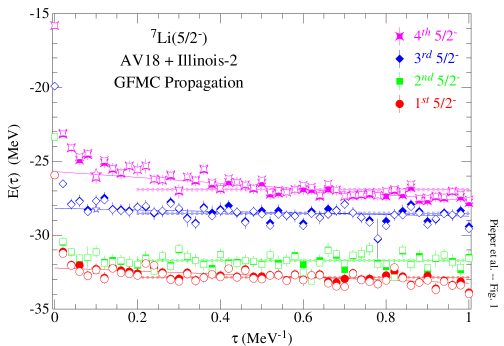
Figure 1: (Color online) GFMC energies of four $\frac{5}{2}^{-}$ states in ⁷Li versus imaginary time, $\tau$. The solid symbols show the computed energies at each $\tau$; open symbols show the results of the rediagonalization discussed in the text.

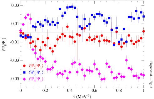
Figure 2: (Color online) Overlaps of the GFMC wave functions for the first $\frac{5}{2}^{-}$ state in ⁷Li with the other three $\frac{5}{2}^{-}$ states versus imaginary time.

As an example, Figs. 1 and 2 show the computation of the energies of four $\frac{5}{2}^{-}$ states in ⁷Li; the $\Psi_{T,i}$ used to start the propagations are defined in Table 4. The diagonal $H_{ii}(\tau)$ are shown as solid symbols in Fig. 1. The lowest state has mainly [43] symmetry and can easily decay to the $\alpha$+t channel; it has a large experimental width (918 keV) and its computed energy is slowly decreasing to the energy of the separated clusters. The remaining states are mainly of [421] symmetry and so are principally connected to the ⁶Li+n channel. The second $\frac{5}{2}^{-}$ state is experimentally just above the ⁶Li+n threshold and has a small width (80 keV); its computed energy becomes constant with increasing $\tau$. The last two $\frac{5}{2}^{-}$ states are not experimentally known, but the very slow decrease with $\tau$ of the energy of the third state suggests that this state may also be narrow. Figure 2 shows the off-diagonal overlaps $N_{i1}(\tau)$; they are small and do not show signs of steadily increasing with increasing $\tau$. The $N_{i\neq j}(\tau\!=\!0)$ are not identically zero because the diagonalization that determined the $\beta_{LS[n]}$ was made in a different Monte Carlo walk from the ones generating the $N_{ij}$. These results show that the (constrained) GFMC propagation largely retains the orthogonality of the starting $\Psi_{T,i}$. Contrary to what might have been expected, the propagation of the higher states does not quickly collapse to the lowest state.

The open symbols in Fig. 1 show the results of generalized eigenvalue calculations made for each $\tau$ using the $H_{ij}(\tau)$ and $N_{ij}(\tau)$. As is expected from the small overlaps, there is no statistically significant change of the rediagonalized energies from the directly computed $H_{ii}(\tau)$. Based on this result and the generally constant $H_{ii}(\tau)$ that we obtain for other cases, we use the $H_{ii}(\tau)$ directly without making a final rediagonalization.

V Numerical results for $A$ = 6 to 8 nuclei

Figure 1 shows that for some unbound cases the GFMC energy never stabilizes, but rather slowly decays with increasing $\tau$. In these cases a linear fit with non-zero slope provides a much lower $\chi^{2}$ fit to the $E(\tau)$ for large $\tau$ than does a constant fit. We use this linear fit to extrapolate back to $\tau\approx 0.08$ because it appears that the GFMC calculations for bound systems have all become stable by $\tau\approx 0.08$. Such extrapolated values are printed in italics in the tables; they must be considered as less reliable than the non-italicized values.

Table 8: Energies and excitation energies (MeV) of selected nuclear states calculated for the AV18/UIX Hamiltonian by VMC and GFMC. Monte Carlo statistical errors in the last digits are shown in parentheses. See the text for italicized GFMC values.

	Energy		Excitation Energy
	VMC	GFMC	VMC	GFMC
4He(0+)	$-$27.39(3)	$-$28.31(2)
6He(0+)	$-$24.79(9)	$-$28.02(9)
6He(2+)	$-$23.07(9)	$-$26.08(9)	1.7(1)	1.9(1)
6He(1+)	$-$20.72(9)	$-$23.9(2)	4.1(1)	4.2(2)
6Li(1+)	$-$27.96(8)	$-$31.25(8)
6Li(3+)	$-$25.05(9)	$-$28.45(8)	2.9(1)	2.8(1)
6Li(2+)	$-$23.8(1)	$-$27.25(8)	4.2(1)	4.0(1)
6Li(1+, 2nd)	$-$22.69(8)	$-$26.2(1)	5.3(1)	5.1(1)
7He($\frac{3}{2}^{-}$)	$-$20.93(8)	$-$26.3(1)
7He($\frac{1}{2}^{-}$)	$-$18.8(1)	$-$25.2(1)	2.1(1)	1.1(1)
7He($\frac{5}{2}^{-}$)	$-$18.33(9)	$-$23.9(1)	2.6(1)	2.5(2)
7Li($\frac{3}{2}^{-}$)	$-$33.0(3)	$-$37.5(1)
7Li($\frac{1}{2}^{-}$)	$-$32.9(1)	$-$37.6(1)	.1(3)	$-$.1(2)
7Li($\frac{7}{2}^{-}$)	$-$27.2(1)	$-$32.2(1)	5.8(3)	5.3(1)
7Li($\frac{5}{2}^{-}$)	$-$26.61(9)	$-$31.1(1)	6.4(3)	6.5(2)
7Li($\frac{5}{2}^{-}$, 2nd)	$-$23.7(1)	$-$29.7(2)	9.3(3)	7.8(2)
7Li($\frac{3}{2}^{-}$, 2nd)	$-$22.8(1)	$-$29.1(2)	10.2(3)	8.5(3)
7Li($\frac{7}{2}^{-}$, 2nd)	$-$21.8(1)	$-$28.1(2)	11.2(3)	9.5(2)
7Li($\frac{5}{2}^{-}$, 3rd)	$-$20.5(1)	$-$27.0(2)	12.5(3)	10.5(2)
7Li($\frac{5}{2}^{-}$, 4th)	$-$16.8(2)	$-$24.4(5)	16.2(4)	13.1(5)
8He(0+)	$-$20.75(7)	$-$27.7(1)
8He(2+)	$-$18.2(1)	$-$25.0(1)	2.5(1)	2.8(2)
8He(1+)	$-$17.56(8)	$-$23.3(3)	3.2(1)	4.4(3)
8Li(2+)	$-$30.7(1)	$-$38.8(1)
8Li(1+)	$-$29.6(1)	$-$37.8(2)	1.1(1)	1.0(2)
8Li(0+)	$-$28.6(1)	$-$36.9(1)	2.1(1)	2.0(2)
8Li(3+)	$-$27.24(9)	$-$35.4(1)	3.5(1)	3.4(2)
8Li(1+, 2nd)	$-$27.7(1)	$-$35.2(1)	3.0(2)	3.6(2)
8Li(4+)	$-$24.42(9)	$-$32.3(2)	6.3(1)	6.5(2)
8Be(0+)	$-$48.6(1)	$-$55.2(1)
8Be(2+)	$-$45.71(9)	$-$52.1(2)	2.9(1)	3.1(3)
8Be(4+)	$-$37.59(9)	$-$44.2(5)	11.0(1)	11.0(5)
8Be(1+)	$-$28.07(8)	$-$37.0(2)	20.6(1)	18.2(2)
8Be(2+, 2nd)	$-$28.8(1)	$-$36.4(6)	19.8(1)	18.9(6)
8Be(3+)	$-$26.69(7)	$-$35.2(2)	21.9(1)	20.0(2)

Selected VMC and GFMC energies computed for the AV18/UIX Hamiltonian are shown in Table 8. The VMC energies for the $\Psi_{T}$ of Eq. (1) are significantly improved compared to those reported in Refs. PPCPW97 ; WPCP00 . The ⁴He energy has been lowered by 0.4 MeV, the $A$=6 energies by 1 MeV, the $A$=7 energies by 2 MeV, and the $A=8$ energies by 2.75 MeV. Compared to the more sophisticated (and more expensive) $\Psi_{V}$ of Refs. PPCPW97 ; WPCP00 , which includes spin-orbit and additional three-body correlations, the energies from the present $\Psi_{T}$ are as good for $A$=6 and even better for $A$=7,8.

Table 9: $A$ = 4, 6 and 7 GFMC energies for the AV8^′, AV18, and AV18/IL2 Hamiltonians compared with experimental values exp567 . Except as noted, states have the same isospin as the corresponding ground state. Square brackets enclose experimental energies which have uncertain $J^{\pi}$ assignments. See the text for italicized GFMC values. All values are in MeV.

	AV8′	AV18	AV18/IL2	Experiment
				Energy	Width
4He(0+)	$-$25.14(2)	$-$24.07(4)	$-$28.37(3)	$-$28.30(0)
6He(0+)	$-$25.11(3)	$-$23.8(1)	$-$29.28(2)	$-$29.27
6He(2+)	$-$23.21(4)	$-$21.9(1)	$-$27.3(2)	$-$27.47(3)	0.113
6He(2+, 2nd)	$-$21.4(1)	$-$20.4(1)	$-$24.6(1)
6He(1+)	$-$21.0(1)	$-$19.6(2)	$-$24.5(1)
6He(0+, 2nd)	$-$20.15(6)	$-$19.0(1)	$-$23.3(1)
6Li(1+)	$-$28.15(3)	$-$26.9(1)	$-$32.0(1)	$-$31.99
6Li(3+)	$-$25.33(3)	$-$24.1(1)	$-$29.8(1)	$-$29.80	0.024
6Li(0+, $T$=1)	$-$24.31(3)	$-$23.0(1)	$-$28.6(1)	$-$28.43
6Li(2+)	$-$24.18(5)	$-$22.8(1)	$-$27.8(1)	$-$27.68(2)	1.3
6Li(2+, $T$=1)	$-$22.48(4)	$-$21.1(1)	$-$26.5(1)	$-$26.62	0.54
6Li(1+, 2nd)	$-$23.19(6)	$-$22.0(1)	$-$26.4(2)	$-$26.34(5)	1.5
6Li(1+, 3rd)	$-$19.7(2)	$-$18.8(1)	$-$23.4(1)
7He($\frac{3}{2}^{-}$)	$-$23.39(7)	$-$21.9(1)	$-$28.8(2)	$-$28.82(3)	0.16
7He($\frac{1}{2}^{-}$)	$-$22.05(9)	$-$20.7(1)	$-$25.9(2)
7He($\frac{5}{2}^{-}$)	$-$20.8(1)	$-$19.4(1)	$-$25.5(1)	[$-$25.90(10)]	1.99
7He($\frac{3}{2}^{-}$, 2nd)			$-$25.0(1)
7He($\frac{3}{2}^{-}$, 3rd)			$-$21.7(3)
7Li($\frac{3}{2}^{-}$)	$-$33.86(4)	$-$32.0(1)	$-$38.9(1)	$-$39.24
7Li($\frac{1}{2}^{-}$)	$-$33.95(4)	$-$32.2(1)	$-$38.7(1)	$-$38.76
7Li($\frac{7}{2}^{-}$)	$-$28.6(1)	$-$26.8(2)	$-$34.0(1)	$-$34.59(1)	0.069
7Li($\frac{5}{2}^{-}$)	$-$28.11(6)	$-$26.4(1)	$-$32.3(1)	$-$32.64(5)	0.92
7Li($\frac{5}{2}^{-}$, 2nd)	$-$26.42(7)	$-$24.5(1)	$-$31.7(1)	$-$31.79	0.08
7Li($\frac{3}{2}^{-}$, 2nd)	$-$25.4(2)	$-$24.4(1)	$-$29.7(1)	$-$30.49	4.7
7Li($\frac{1}{2}^{-}$, 2nd)	$-$25.37(7)	$-$23.8(1)	$-$29.1(2)	$-$30.15	2.8
7Li($\frac{7}{2}^{-}$, 2nd)	$-$24.59(7)	$-$23.0(1)	$-$29.2(2)	$-$29.67(10)	0.44
7Li($\frac{5}{2}^{-}$, 3rd)			$-$28.6(1)
7Li($\frac{5}{2}^{-}$, 4th)			$-$25.8(1)

Table 10: $A$ = 8 GFMC energies for the AV8^′, AV18, and AV18/IL2 Hamiltonians compared with experimental values exp8 . Conventions are the same as in Table 9. The $2^{+}$ states near $-39.7$ MeV in ⁸Be are strongly isospin mixed; their experimental energies, marked with an asterisk, have not been corrected for this effect.

	AV8′	AV18	AV18/IL2	Experiment
				Energy	Width
8He(0+)	$-$24.3(1)	$-$23.0(1)	$-$31.72(4)	$-$31.41(1)
8He(2+)	$-$21.93(6)	$-$20.4(1)	$-$27.0(2)	$-$28.31(50)	0.6
8He(1+)	$-$20.3(2)	$-$18.8(3)	$-$25.9(2)
8He(0+, 2nd)			$-$24.8(2)
8He(2+, 2nd)			$-$23.7(2)
8Li(2+)	$-$34.74(6)	$-$32.7(1)	$-$41.9(2)	$-$41.28
8Li(1+)	$-$34.34(7)	$-$32.1(1)	$-$40.5(2)	$-$40.30
8Li(3+)	$-$32.16(7)	$-$30.1(2)	$-$39.4(2)	$-$39.02	0.033
8Li(0+)	$-$33.51(6)	$-$31.5(1)	$-$38.3(2)
8Li(1+, 2nd)	$-$32.76(7)	$-$31.0(1)	$-$37.2(2)	$-$38.07	1.
8Li(2+, 2nd)	$-$31.2(2)	$-$29.7(1)	$-$36.6(4)
8Li(2+, 3rd)	$-$30.49(7)	$-$28.7(2)	$-$36.9(2)
8Li(1+, 3rd)	$-$31.14(7)	$-$29.1(2)	$-$35.9(2)	[$-$35.88]	0.65
8Li(3+, 2nd)	$-$28.47(7)	$-$26.3(1)	$-$33.8(2)	[$-$35.18(10)]	1.
8Li(4+)	$-$29.1(1)	$-$27.1(1)	$-$34.7(2)	$-$34.75(2)	0.035
8Be(0+)	$-$48.95(7)	$-$46.3(2)	$-$56.3(1)	$-$56.50
8Be(2+)	$-$45.6(3)	$-$43.7(2)	$-$52.2(2)	$-$53.44(3)	1.4
8Be(4+)	$-$37.7(5)	$-$36.2(2)	$-$45.4(3)	$-$45.15(15)	3.5
8Be(2+, $T$=1)	$-$33.40(6)	$-$31.2(1)	$-$40.4(2)	$-39.87^{*}$	0.108
8Be(2+, 2nd)	$-$33.41(9)	$-$31.0(2)	$-$39.8(3)	$-39.58^{*}$	0.074
8Be(1+, $T$=1)	$-$33.03(7)	$-$30.7(1)	$-$39.0(2)	$-$38.86	0.011
8Be(1+)	$-$33.25(9)	$-$30.8(2)	$-$39.4(3)	$-$38.35	0.138
8Be(3+, $T$=1)	$-$30.87(7)	$-$28.8(2)	$-$38.0(2)	$-$37.43	0.27
8Be(1+, 2nd)			$-$37.3(3)
8Be(3+)	$-$31.68(9)	$-$29.7(2)	$-$37.2(1)	$-$37.26(1)	0.23
8Be(4+, 2nd)			$-$37.6(3)	$-$36.64(5)	0.7
8Be(2+, 3rd)	$-$31.49(9)	$-$29.1(2)	$-$37.0(3)	$-$36.40	0.88
8Be(0+, 2nd)			$-$36.0(3)	$-$36.30	0.72
8Be(3+, 2nd)			$-$34.0(3)	$-$35.00	1.
8Be(2+, 4th)			$-$34.0(3)	$-$34.30	0.8

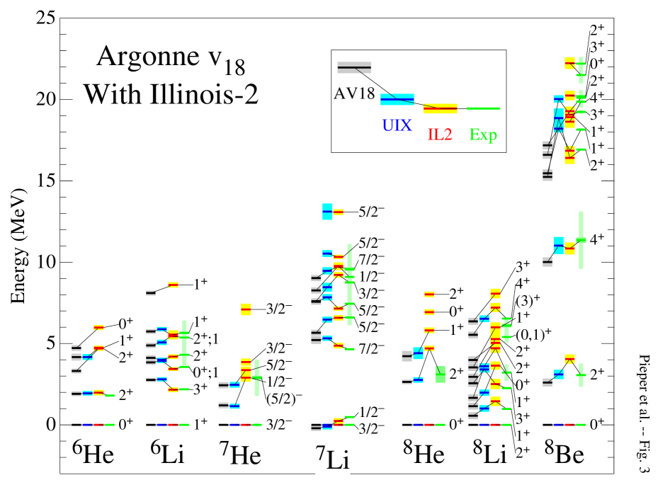
Figure 3: (Color online) GFMC excitation energies computed for the AV18, AV18/UIX, and AV18/IL2 Hamiltonians compared with experimental values. The shaded bands show the Monte Carlo statistical (or experimental) errors. The narrow shaded bars on the experimental values show the experimental widths.

The improvements are due primarily to 1) improved shapes for the two-body tensor correlation functions $u_{t}(r)$, $u_{t\tau}(r)$ contained in $U_{ij}$ [Eq. (3)], including allowing them to be different for s-shell and p-shell nuclei, 2) letting the $f_{sp}(r)$ vary with the $LS[n]$ wave function component, and 3) using more extended $f_{sp}(r)$ and $f_{pp}(r)$ which allow the overall wave function to be more diffuse. In particular, the lack of experimental charge radii for $A$=8 nuclei makes it difficult to fix the optimal size of these wave functions; in the present case the matter radii for the ground states have been adjusted to match the earlier GFMC results of Ref. WPCP00 .

Many of the GFMC results in Table 8 have changed by 1 to 3 standard deviations from the results reported in Ref. PPWC01 . However, the quoted errors are statistical only; we have previously estimated PPCPW97 ; WPCP00 the systematic errors to be of the order of 1-2%, and the changes reported here are within that range. The changes are due to the improved treatment of $V_{ijk}$ discussed above, propagation to larger $\tau$, and in some cases improved $\beta_{LS[n]}$ choices. These changes are significantly less than the corresponding improvements in the $\Psi_{T}$ values, indicating that (aside from modifications of the $\beta_{LS[n]}$) high-energy contaminations have been removed from the $\Psi_{T}$; these were previously easily corrected by the GFMC.

For the p-shell nuclei, the improved $\Psi_{T}$ energies are still 10 to 20% higher than the GFMC values. However the excitation energies computed with the $\Psi_{T}$ are generally quite accurate, providing the states are dominated by the same spatial symmetry as the ground state. The second $\frac{5}{2}^{-}$ and higher states of ⁷Li and the $1^{+}$ and $3^{+}$ states of ⁸Be have lower spatial symmetry than the corresponding ground states and their VMC excitation energies are significantly too high; we also see this pattern in the VMC energies of other higher states and with other Hamiltonians.

Tables 9 and 10 give GFMC energies for the AV8^′, AV18, and AV18/IL2 Hamiltonians and also show the experimental energies and widths of the states that have been observed (widths less than 0.01 MeV are not shown). Figure 3 shows the corresponding excitation energies. The values for second or higher states of a given $J^{\pi}$ are presented here for the first time, however the other values have all been recomputed with, in many cases, increased maximum $\tau$, improved determinations of the $\beta_{LS[n]}$ in the $\Psi_{T}$, and improved treatment of the $V_{ijk}$ in the propagation. For these reasons, some of the values are significantly different from previously published values.

The AV18/IL2 Hamiltonian was originally determined by making a three-parameter fit to 17 states in the $A$ = 3 to 8 region PPWC01 . There are 36 states with $6\leq A\leq 8$ that have experimental energies in Tables 9 and 10. The RMS error in predicting the energies of these states is only 0.60 MeV; the RMS error for just the 17 states with widths less than 0.2 MeV is 0.38 MeV and the RMS error for the 7 ground-state energies is 0.31 MeV. The RMS errors in excitation energies are 0.76 MeV for all 29 excited states and 0.54 MeV for the 10 narrow states. Analog states have been omitted from all of these averages but the states with uncertain experimental $J^{\pi}$ assignments were included; omitting the latter does not substantially change the above numbers. These results are basically the same as the RMS errors reported for 26 states in Ref. PPWC01 .

Table 11: GFMC expectation values of $V_{ijk}$ for the AV18/IL2 Hamiltonian

	$V^{2\pi}$	$V^{3\pi}$	$V^{R}$	$V_{ijk}$
4He	$-$16.3(1)	0.63(1)	7.3(1)	$-$8.4(1)
6He	$-$18.9(1)	$-$0.58(1)	8.9(1)	$-$10.6(1)
6Li	$-$20.1(2)	$-$0.09(3)	9.4(2)	$-$10.8(2)
7He	$-$23.5(3)	$-$2.22(6)	11.6(2)	$-$14.2(2)
7Li	$-$24.9(2)	$-$0.50(3)	11.7(1)	$-$13.7(2)
8He	$-$27.0(1)	$-$4.36(2)	13.8(1)	$-$17.5(1)
8Li	$-$31.4(3)	$-$2.6(1)	15.8(2)	$-$18.2(3)
8Be	$-$35.9(2)	0.32(3)	16.4(2)	$-$19.2(2)

Extensive breakdowns of the total energies were presented in Ref. PPWC01 . The improved treatment of $V_{ijk}$ in the GFMC propagation has resulted in significant changes to the expectation values of $V_{ijk}$ and its components for the AV18/IL2 Hamiltonian; revised values are shown in Table 11. The other contributions to the total energies shown in Ref. PPWC01 are not significantly changed. The isovector and isotensor energies presented there have also not significantly changed in the current calculations. Tables 9 and 10 contain energies of a few $T$=1 states for ⁶Li and ⁸Be; these have been computed perturbatively using the isovector and isotensor energies computed for ⁶He and ⁸Li, respectively. Recently we have realized that there is a significant difficulty in extracting precise RMS radii from GFMC calculations, especially for weakly bound systems. For this reason we are deferring presenting updated values for the RMS radii.

VI Conclusions

We have demonstrated that it is possible to use GFMC to compute the energies of multiple nuclear states with the same quantum numbers. This substantially increases the number of nuclear level energies that can be compared to experimental values in the light p-shell region. The AV18/IL2 Hamiltonian presented in Ref. PPWC01 gives a good description of this increased set of energies. We are currently extending these calculations to higher excited states in the $A$=9,10 nuclei.

We have also improved our treatment of the three-nucleon force in the GFMC calculations. This has altered the detailed breakdown of $N\!N\!N$ contributions as shown in Table 11. We expect a similar alteration of these terms in the $A$=9,10 nuclei, but the total energies should stay within 1-2% of our previously reported values PVW02 .

- (1) Electronic address: spieper@anl.gov
- (2) Electronic address: wiringa@anl.gov
- (3) Electronic address: carlson@lanl.gov
- (4) B. S. Pudliner, V. R. Pandharipande, J. Carlson, and R. B. Wiringa, Phys. Rev. Lett. 74, 4396 (1995).
- (5) B. S. Pudliner, V. R. Pandharipande, J. Carlson, S. C. Pieper, and R. B. Wiringa, Phys. Rev. C 56, 1720 (1997).
- (6) R. B. Wiringa, S. C. Pieper, J. Carlson, and V. R. Pandharipande, Phys. Rev. C 62, 014001 (2000).
- (7) S. C. Pieper, V. R. Pandharipande, R. B. Wiringa, and J. Carlson, Phys. Rev. C 64, 014001 (2001).
- (8) S. C. Pieper, K. Varga, and R. B. Wiringa, Phys. Rev. C 66, 044310 (2002).
- (9) R. B. Wiringa, V. G. J. Stoks, and R. Schiavilla, Phys. Rev. C 51, 38 (1995).
- (10) R. B. Wiringa, Phys. Rev. C 43, 1585 (1991).
- (11) S. Cohen and D. Kurath, Nucl. Phys. 73, 1 (1965).
- (12) A. Bohr and B. R. Mottelson, Nuclear Structure Volume I, (W. A. Benjamin, New York, 1969), Appendix 1C.
- (13) D. R. Tilley, C. M. Cheves, J. L. Godwin, G. M. Hale, H. M. Hofmann, J. H. Kelley, C. G. Sheu, and H. R. Weller, Nucl. Phys. A708, 3 (2002).
- (14) J. H. Kelley, J. L. Godwin, X. Hu, J. Purcell, C. G. Sheu, D. R. Tilley, and H. R. Weller, preprint (2002); on-line version at www.tunl.duke.edu/nucldata/chain/08.shtml.