Novel $NN$ interaction and the spectroscopy of light nuclei

Abstract

Nucleon-nucleon ($NN$) phase shifts and the spectroscopy of $A\leq 6$ nuclei are successfully described by an inverse scattering potential that is separable with oscillator form factors.

Nucleon-nucleon ($NN$) potentials that describe available two-body data have a long and multi-faceted history. High precision fits have improved with time even as more precise experimental data have become available. Three-nucleon ($NNN$) potentials have a shorter history but are intensively investigated at the present time. Disparate foundations for these potentials, both $NN$ & $NNN$, have emerged. On the one hand, one sees the predominant meson-exchange potentials sometimes supplemented with phenomenological terms to achieve high accuracy in fitting $NN$ data (Bonn Bonn , Nijmegen Stocks , Argonne Argonne , Idaho Idaho , IS Plessas ) and $NNN$ data (Urbana Urbana ; GFMC , Illinois Illinois , Tucson–Melbourne TM ; TM-pr ). On the other hand, one sees the emergence of potentials with ties to QCD which are either meson-free vanKolck , or intertwined with meson-exchange theory Bochum ; Idaho .

All these potentials are being used, with unprecedented success, to explain a vast amount of data on light nuclei in Quantum Monte Carlo approaches GFMC and ab initio no-core shell model (NCSM) Vary ; Vary3 . The overwhelming success of these efforts have led some to characterize these approaches as leading to a ‘Standard Model’ of non-relativistic nuclear physics.

Chief among the outstanding challenges is the computational intensity of using these $NN+NNN$ potentials within the presently available many-body methods. For this reason, most ab initio investigations have been limited to $A\leq 12$. The situation would be dramatically simpler if either the $NN$ potential alone would be sufficient or the potentials would couple less strongly between the low momentum and the high momentum degrees of freedom. If both simplifications are obtained, the future for applications is far more promising.

In the present work, we derive and apply a new class of potentials which have no apparent connection with the two well-established lines of endeavor. We develop $J$-matrix inverse scattering potentials (JISP) that describe $NN$ data to high accuracy and, with the off-shell freedom that remains, we obtain excellent fits to the bound and resonance states of light nuclei up to $A=6$. Our $NN$ off-shell freedom is sufficient to describe these limited data without the need for $NNN$ potentials. As an important side benefit, we find that these potentials lead to rapid convergence in the ab initio NCSM evaluations presented here. We hope that these potentials will open a fruitful path for evaluating heavier systems and spur the development of extensions to scattering problems.

It is important to stress that our $NN$ potentials have the same symmetries as the conventional $NN$ potentials mentioned above (without charge symmetry breaking at present), but they are not constrained by meson exchange theory, by QCD or by locality. This does not mean our $NN$ potentials are inconsistent with those constraints, however.

By means of the $J$-matrix inverse scattering approach ISTP we construct $NN$ potentials as matrices in an oscillator basis with $\hbar\omega=40$ MeV using the Nijmegen $np$ phase shifts NNonline . Following Ref. ISTP , we obtain inverse scattering tridiagonal potentials (ISTP) that are tridiagonal (quasi-tridiagonal) in uncoupled (coupled) partial waves. The dimension of the potential matrix is specified by the maximum value of $N=2n+l$ and is referred to as an $N\hbar\omega$ potential. In order to improve the description of the phase shifts, we develop a $9\hbar\omega$-ISTP in odd waves instead of the $7\hbar\omega$-ISTP of Ref. ISTP . We retain an $8\hbar\omega$-ISTP in the even partial waves.

Next we perform various phase equivalent transformations (PETs) of the obtained ISTP. In the coupled $sd$ waves, we perform the same PET as in Ref. ISTP but with different rotation angle $\vartheta=11.3^{\circ}$ to improve the description of the deuteron quadrupole moment $Q$. We then find improvement in ³H and ⁴He binding energies. We also perform similar PETs mixing lowest oscillator basis states in the ${}^{3}p_{2}$, ${}^{3}p_{1}$, ${}^{3}d_{2}$ and ${}^{1}p_{1}$ waves with the rotation angles of $\vartheta=+8^{\circ}$, $-6^{\circ}$, $+25^{\circ}$ and $-16^{\circ}$ respectively to improve the description of the ⁶Li spectrum. The obtained interaction fitted to the spectrum of $A=6$ nuclei, is refered to as JISP6. The non-zero matrix elements of the JISP6 interaction are presented in Tables 4–10 (in $\hbar\omega=40$ MeV units).

Table 1: Non-zero matrix elements in $\hbar\omega=40$ MeV units of the JISP6 matrix in the ${}^{1}s_{0}$ partial wave.

$n$	$V_{nn}^{l}$	$V_{n,\,n+1}^{l}=V_{n+1,\,n}^{l}$
$0$	$-0.370829835410$	$0.132663053234$
$1$	$-0.148826473896$	$0.006448104375$
$2$	$0.152835073179$	$-0.120193538281$
$3$	$0.187138532148$	$-0.029504403821$
$4$	$-0.005584124194$

Table 2: Non-zero matrix elements in $\hbar\omega=40$ MeV units of the JISP6 matrix in the ${}^{1}p_{1}$ partial wave.

$n$	$V_{nn}^{l}$	$V_{n,\,n+1}^{l}=V_{n+1,\,n}^{l}$	$V_{n,\,n+2}^{l}=V_{n+2,\,n}^{l}$
$0$	$0.631081576474$	$-0.251382936855$	$0.413319237868$
$1$	$-0.293390247307$	$-0.118539824524$
$2$	$0.454133632867$	$-0.230186013455$
$3$	$0.348035837559$	$-0.090043227032$
$4$	$0.049221178231$

Table 3: Non-zero matrix elements in $\hbar\omega=40$ MeV units of the JISP6 matrix in the ${}^{1}d_{2}$ partial wave.

$n$	$V_{nn}^{l}$	$V_{n,\,n+1}^{l}=V_{n+1,\,n}^{l}$
$0$	$-0.040699390045$	$0.037531685348$
$1$	$-0.111761745807$	$0.069791608541$
$2$	$-0.134996618188$	$0.045265020638$
$3$	$-0.031270631267$

Table 4: Non-zero matrix elements in $\hbar\omega=40$ MeV units of the JISP6 matrix in the ${}^{1}f_{3}$ partial wave.

$n$	$V_{nn}^{l}$	$V_{n,\,n+1}^{l}=V_{n+1,\,n}^{l}$
$0$	$0.019468932284$	$-0.018631285428$
$1$	$0.083569595544$	$-0.055488297878$
$2$	$0.106821875609$	$-0.032273326919$
$3$	$0.021063860199$

Table 5: Non-zero matrix elements in $\hbar\omega=40$ MeV units of the JISP6 matrix in the ${}^{3}p_{0}$ partial wave.

$n$	$V_{nn}^{l}$	$V_{n,\,n+1}^{l}=V_{n+1,\,n}^{l}$
$0$	$-0.143164548564$	$0.020755069079$
$1$	$0.082988173615$	$-0.120094506156$
$2$	$0.310447079465$	$-0.116102071897$
$3$	$0.065044984944$	$0.013609203897$
$4$	$-0.026555044004$

Table 6: Non-zero matrix elements in $\hbar\omega=40$ MeV units of the JISP6 matrix in the ${}^{3}p_{1}$ partial wave.

$n$	$V_{nn}^{l}$	$V_{n,\,n+1}^{l}=V_{n+1,\,n}^{l}$	$V_{n,\,n+2}^{l}=V_{n+2,\,n}^{l}$
$0$	$0.249679784904$	$-0.164761352606$	$0.157602869176$
$1$	$0.044327922667$	$-0.176615480839$
$2$	$0.514099248363$	$-0.275733929941$
$3$	$0.423324941377$	$-0.108223480414$
$4$	$0.055397268090$

Table 7: Non-zero matrix elements in $\hbar\omega=40$ MeV units of the JISP6 matrix in the ${}^{3}d_{2}$ partial wave.

$n$	$V_{nn}^{l}$	$V_{n,\,n+1}^{l}=V_{n+1,\,n}^{l}$	$V_{n,\,n+2}^{l}=V_{n+2,\,n}^{l}$
$0$	$-0.662113235725$	$0.759732268972$	$-0.571851583929$
$1$	$0.175448232529$	$0.273660320760$
$2$	$-0.263880156721$	$0.086029122705$
$3$	$-0.063231092747$

Table 8: Non-zero matrix elements in $\hbar\omega=40$ MeV units of the JISP6 matrix in the ${}^{3}f_{3}$ partial wave.

$n$	$V_{nn}^{l}$	$V_{n,\,n+1}^{l}=V_{n+1,\,n}^{l}$
$0$	$0.026326206898$	$-0.014285757490$
$1$	$0.035674429367$	$-0.016797566427$
$2$	$0.028543592124$	$-0.008290586001$
$3$	$0.006036946613$

Table 9: Non-zero matrix elements in $\hbar\omega=40$ MeV units of the JISP6 matrix in the $sd$ coupled waves.

$V^{ss}_{nn^{\prime}}$ matrix elements
$n$	$V_{nn}^{ss}$	$V_{n,n+1}^{ss}=V^{ss}_{n+1,n}$
$0$	$-0.508274040822$	$0.214156446587$
$1$	$-0.276168029473$	$0.080907735691$
$2$	$-0.009473803659$	$-0.051881443108$
$3$	$0.152873734289$	$-0.055193589842$
$4$	$0.037547929880$
$V^{dd}_{nn^{\prime}}$ matrix elements
$n$	$V_{nn}^{dd}$	$V_{n,n+1}^{dd}=V^{dd}_{n+1,n}$
$0$	$0.050878349132$	$-0.094173649477$
$1$	$0.322126471805$	$-0.178808793641$
$2$	$0.308516673061$	$-0.093012604766$
$3$	$0.061200037193$
$V^{sd}_{nn^{\prime}}=V^{ds}_{n^{\prime}n}$ matrix elements
$n$	$V_{n,n-1}^{sd}=V^{ds}_{n-1,n}$	$V_{nn}^{sd}=V_{nn}^{ds}$	$V_{n,n+1}^{sd}=V^{ds}_{n+1,n}$
$0$		$-0.411771355351$	$0.205731982741$
$1$	$-0.048516342749$	$-0.060476585693$
$2$	$0.068044496963$	$-0.080187106458$
$3$	$0.049400578816$	$-0.020205646231$
$4$	$-0.001503998139$

Table 10: Non-zero matrix elements in $\hbar\omega=40$ MeV units of the JISP6 matrix in the $pf$ coupled partial waves.

$V^{pp}_{nn^{\prime}\vphantom{,}}$ matrix elements
$n$	$V_{nn}^{pp}$	$V_{n,n+1}^{pp}=V_{n+1,n}^{pp}$	$V_{n,n+2}^{pp}=V_{n+2,n}^{pp}$
$0$	$-0.257052769018$	$0.215269922150$	$-0.171332097424$
$1$	$0.035950531483$	$0.103784437050$
$2$	$-0.209221226255$	$0.103221679634$
$3$	$-0.151546344031$	$0.037329967115$
$4$	$-0.015878201100$
$V^{ff}_{nn^{\prime}\vphantom{,}}$ matrix elements
$n$	$V_{nn}^{ff}$	$V_{n,n+1}^{ff}=V_{n+1,n}^{ff}$
$0$	$-0.019836117401$	$0.008292672214$
$1$	$-0.010058323807$	$0.000628665253$
$2$	$0.001646202464$	$-0.000973797731$
$3$	$0.000388504318$
$V^{pf}_{nn^{\prime}\vphantom{,}}$ matrix elements
$n$	$V_{n,n-1}^{pf}=V_{n-1,n}^{fp}$	$V_{nn}^{pf}=V^{fp}_{nn}$	$V_{n,n+1}^{pf}=V^{fp}_{n+1,n}$
$0$		$0.018163699530$	$0.003299666393$
$1$	$-0.026186898553$	$0.023478346345$
$2$	$-0.024757588981$	$0.023707438623$
$3$	$-0.014708906826$	$0.006271279847$
$4$	$0.000024653107$

The deuteron properties provided by JISP6 are compared with those of some other realistic potentials in Table 11.

Table 11: JISP6 deuteron property predictions in comparison with the ones obtained with various realistic potentials.

Potential	$E_{d}$, MeV	$d$ state probability, %	rms radius, fm	$Q$, fm2	As. norm. const. ${\mathscr{A}}_{s}$, fm-1/2	$\displaystyle\eta=\frac{{\mathscr{A}}\vphantom{{}^{\prime}}_{d}}{{\mathscr{A}}_{s\vphantom{{}_{a}}}}$
JISP6	$-2.224575$	4.1360	1.9647	0.2915	0.8629	0.0252
Nijmegen-II	$-2.224575$	5.635	1.968	0.2707	0.8845	0.0252
AV18	$-2.224575$	5.76	1.967	0.270	0.8850	0.0250
CD–Bonn	$-2.224575$	4.85	1.966	0.270	0.8846	0.0256
Nature	$-2.224575(9)$	—	1.971(6)	0.2859(3)	0.8846(9)	0.0256(4)

We perform calculations of light nuclei in the NCSM with JISP6 plus the Coulomb interaction between protons. To improve the convergence, we perform the Lee–Suzuki transformation to obtain a two-body effective interaction as is discussed in Ref. Vary3 . We obtain the effective interaction in a new basis ($\hbar\omega=15$ MeV) within an $N_{max}\hbar\omega$ model space where $N_{max}$ signifies the many-body oscillator basis cutoff. The results of our NCSM calculations for binding energies of ³H,³He (in the $14\hbar\omega$ model space), ⁴He (in the $12\hbar\omega$ model space), ⁶He (in the $8\hbar\omega$ model space) and ⁶Li (in the $10\hbar\omega$ model space) nuclei are compared in Table 12 with the calculations in various approaches [Faddeev, Green’s-function Monte Carlo (GFMC), NCSM] with realistic $NN$ [CD-Bonn, Nijmegen-I (NijmI), Nijmegen-II (NijmII), and Argonne (AV18 and AV8’)] and $NNN$ [Urbana (UrbIX) and Tucson–Melbourne (TM and TM’)] potentials. To give an estimate of the convergence of our calculations, we present the difference between the given result and the result obtained in the next smaller model space in parenthesis after our JISP6 results. It is seen that the convergence of our calculations is adequate.

Table 12: The binding energies of ³H,³He, ⁴He, ⁶He and ⁶Li nuclei.

Potential	3H	3He	4He	6He	6Li
JISP6, NCSM	8.461(5)	7.751(3)	28.611(41)	29.072(69)	31.48(27)
CD-Bonn+TM, Faddeev alpha	8.480	7.734	29.15
AV18+TM, Faddeev alpha	8.476	7.756	28.84
AV18+TM, Faddeev alpha	8.444	7.728	28.36
NijmI+TM, Faddeev alpha	8.392	7.720	28.60
NijmII+TM, Faddeev alpha	8.386	7.720	28.54
AV18+UrbIX, Faddeev alpha	8.478	7.760	28.50
AV18+UrbIX, GFMC GFMC	8.47(1)		28.30(2)	27.64(14)	31.25(11)
AV8’+TM’, NCSM NaO				28.189	31.036
Nature	8.48	7.72	28.30	29.269	31.995

The convergence patterns are also illustrated by Fig. 1 where we present the $\hbar\omega$ dependence of the ⁶Li ground state energy in comparison with the results of Ref. NVOB obtained in NCSM with CD-Bonn interaction. The $\hbar\omega$ dependence with the JISP6 interaction is weaker over a wide interval of $\hbar\omega$ values. This is a signal that convergence is improved relative to CD-Bonn. The variational principle cannot be applied to the NCSM calculations with effective interactions so the convergence may be either from above or below. However, we may surmise that the residual contributions of neglected three-body effective interactions is more significant in the CD-Bonn case.

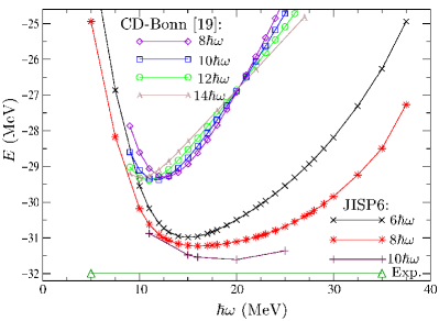
Figure 1: (Color online) $\hbar\omega$ dependence of the ⁶Li ground state energy obtained with JISP6 interaction in comparison with the one obtained in NCSM with CD-Bonn potential NVOB .

Returning to the results presented in Tables 11–12, we see that the JISP6 interaction provides a realistic description of the ground states of light nuclei competitive with the quality of descriptions previously achieved with both $NN$ and $NNN$ forces.

This conclusion is supported by the calculations of the spectra of $A=6$ nuclei with $\hbar\omega=15$ MeV presented in Table 13. We again present in parenthesis the difference between the given excitation energy and the result obtained in the next smaller model space. It is seen that the ⁶Li spectrum is well-reproduced in our calculations. The most important difference with the experiment is the excitation energy of the $(1^{+}_{2},0)$ state. However $E_{x}(1^{+}_{2},0)$ goes down rapidly when the model space is increased and better results are anticipated in a larger model space. The JISP6 results for ⁶Li spectrum are also seen to be competitive with results from modern realistic $NN+NNN$ interaction models. We note here that the ⁶Li spectrum was found NaO to be significantly sensitive to the presence of the $NNN$ force and this motivated our adoption of ⁶Li for these comparisons.

Table 13: Excitation energies $E_{x}$ (in MeV) of $A=6$ nuclei.

6Li	Nature	JISP6	AV8’+TM’	​AV18+UrbIX
​Model space		$10\hbar\omega$	​NCSM, $6\hbar\omega$ NaO	GFMC GFMC
$E_{x}(1^{+}_{1},0)$	0.0	0.0	0.0	0.0
$E_{x}(3^{+},0)$	2.186	2.102(4)	2.471	2.72(36)
$E_{x}(0^{+},1)$	3.563	3.348(24)	3.886	3.94(23)
$E_{x}(2^{+},0)$	4.312	4.642(2)	5.010	4.43(39)
$E_{x}(2^{+},1)$	5.366	5.820(4)	6.482
$E_{x}(1^{+}_{2},0)$	5.65	6.86(36)	7.621
6He	Nature	JISP6	AV8’+TM’	​AV18+UrbIX
​Model space		$8\hbar\omega$	​NCSM, $6\hbar\omega$ NaO	GFMC GFMC
$E_{x}(0^{+},1)$	0.0	0.0	0.0	0.0
$E_{x}(2^{+},1)$	1.8	2.59(13)	2.598	1.80(18)

We return to the underlying rationale for our approach and ask why it is conceivable that an $NN$ interaction alone may be as successful as the $NN+NNN$ potentials mentioned at the outset. That this is feasible may be appreciated from the theorem of Polyzou and Glöckle Poly . They have shown that changing the off-shell properties of two-body potentials is equivalent to adding many-body interactions. This theorem coupled with our limited results suggests that our inverse scattering $NN$ potential plus off-shell modifications is roughly equivalent, for the observables so far investigated, to the successful $NN+NNN$ potential models.

Clearly, more work will be needed to carry this to nuclei with $A\geq 7$ and see if the trend continues. Based on the results presented, the additional off-shell freedoms remaining may well serve to continue this line of fitting properties for some time. When it eventually breaks down, $NNN$ potentials may be needed.

This work was supported in part by RFBR grant No 02-02-17316, by US DOE grant No DE-FG-02 87ER40371 and by US NSF grant No PHY-007-1027.

References

• (1) R. Machleidt, Phys. Rev. CΒ 63, 024001 (2001).
• (2) V. G. J. Stoks et al., Phys. Rev. CΒ 49, 2950 (1994).
• (3) R. B. Wiringa et al., Phys. Rev. CΒ 51, 38 (1995).
• (4) D.Β R.Β Entem and R.Β Machleidt, Phys. Lett. BΒ 524, 93 (2002).
• (5) P. Doleschall et al., Phys. Rev. CΒ 67, 064005 (2003).
• (6) J. Carlson eΝ‘t al., Nucl. Phys. A401, 59 (1983).
• (7) B. S. Pudliner et al., Phys. Rev. CΒ 56, 1720 (1997).
• (8) S. C. Pieper et al., Phys. Rev. CΒ 64, 014001 (1997).
• (9) S. A. Coon et al., Nucl. Phys. AΒ 317, 242 (1979).
• (10) J.Β L.Β Friar et al., Phys. Rev. CΒ 59, 53 (1999); D.Β HΓΌber et al., Few-Body Syst. 30, 95 (2001).
• (11) C. OrdΓ³Γ±ez et al., Phys. Rev. Lett. 72, 1982 (1994); Phys. Rev. CΒ 53, 2086 (1996); U. van Kolck, Phys. Rev. CΒ 49, 2932 (1994).
• (12) E. Epelbaum et al., Phys. Rev. CΒ 66, 064001 (2002); D.Β R.Β Entem and R. Machleidt, Phys. Rev. CΒ 68, 041001 (R) (2003).
• (13) D.Β C. Zheng et al., Phys. Rev. CΒ 50, 2841 (1994); D.Β C.Β Zheng et al., ibid. 52, 2488 (1995).
• (14) P.Β NavrΓ‘til et al., Phys. Rev. Lett. 84, 5728 (2000); Phys. Rev. CΒ 62, 054311 (2000).
• (15) A. M. Shirokov et al., nucl-th/0312029; submitted to Phys. Rev. C.
• (16) http:/​/nn-online.org/.
• (17) A. Nogga et al., Phys. Rev. Lett. 85, 944 (2000).
• (18) P. NavrΓ‘til and E. Ormand, Phys. Rev. C 68, 034305 (2003).
• (19) P. NavrΓ‘til et al., Phys. Rev. Lett. 87, 172502 (2001).
• (20) W. N. Polyzou and W. GlΓΆckle, Few-Body Syst. 9, 97 (1990).