Electromagnetic Form Factors of Hyperons in a Relativistic Quark Model

Abstract

The relativistically covariant constituent quark model developed by the Bonn group is used to compute the EM form factors of strange baryons. We present form-factor results for the ground-state and some excited hyperons. The computed magnetic moments agree well with the experimental values and the magnetic form factors follow a dipole $Q^{2}$ dependence.

1 Motivation

The photo- and electroproduction of mesons from the nucleon is a process in which both electromagnetic and strong interactions occur. One particularly interesting process is the electroproduction of kaons, where a strange quark/antiquark pair is produced from the QCD vacuum. Data from Jefferson Lab have recently been published [1], but an appropriate theoretical description using isobar models is still lacking. One of the main uncertainties in these models is the incompleteness or absence of any knowledge about the form factors, strong or electromagnetic, of the nucleon and hyperon resonances. This work focusses on the latter. We have used the constituent quark (CQ) model developed by the Bonn group to calculate the electromagnetic form factors of ground-state hyperons and the helicity amplitudes of hyperon resonances. The Bonn CQ model is Lorentz covariant and is therefore well suited to describe baryon properties up to high $Q^{2}$, which involve large recoil effects [2].

2 EM Form Factors in the Bethe-Salpeter Approach

2.1 The Bethe-Salpeter Equation

The Bethe-Salpeter (BS) amplitude $\chi_{\overset{\rule{5.69054pt}{0.56905pt}}{P}}$ is the analogue of the wave function in the Hilbert space of three quarks with Dirac, flavor and color degrees of freedom. Starting from the six-point Green’s function, in momentum space, the following integral equation for the BS amplitude can be derived :

$$\chi_{\overset{\rule{5.69054pt}{0.56905pt}}{P}}\;=\;-i\,G_{0\overset{\rule{5.69054pt}{0.56905pt}}{P}}\,\left(K^{(3)}_{\overset{\rule{5.69054pt}{0.56905pt}}{P}}+\overset{\rule{5.69054pt}{0.56905pt}}{K}^{(2)}_{\overset{\rule{5.69054pt}{0.56905pt}}{P}}\right)\,\chi_{\overset{\rule{5.69054pt}{0.56905pt}}{P}}\;.$$ (1)

This expression incorporates all features of the model. It is Lorentz covariant in its inception, and the integral kernel is the product of the free three-quark propagator $G_{0\overset{\rule{5.69054pt}{0.56905pt}}{P}}$ and the sum of all three- and two-particle interactions $K^{(3)}_{\overset{\rule{5.69054pt}{0.56905pt}}{P}}+\overset{\rule{5.69054pt}{0.56905pt}}{K}^{(2)}_{\overset{\rule{5.69054pt}{0.56905pt}}{P}}$. The free three-quark propagator is approximated by the direct product of three free CQ propagators. We use a linear three-quark confinement potential for $K^{(3)}_{\overset{\rule{5.69054pt}{0.56905pt}}{P}}$ and the ’t Hooft instanton induced interaction for $\overset{\rule{5.69054pt}{0.56905pt}}{K}^{(2)}_{\overset{\rule{5.69054pt}{0.56905pt}}{P}}$. Both interactions are assumed to be instantaneous.

Once the BS amplitudes are known, one can calculate any matrix element between two baryon states, provided that the operator is known. When computing electromagnetic form factors, the operator of interest is the electromagnetic current operator. We use the operator $j^{E}_{\mu}=\overset{\rule{5.69054pt}{0.56905pt}}{\Psi}\hat{q}\gamma_{\mu}\Psi$, which describes the photon coupling to a structureless CQ in first order of the electromagnetic interaction. $\Psi$ and $\overset{\rule{5.69054pt}{0.56905pt}}{\Psi}$ are the CQ destruction and creation operators and $\hat{q}$ is the CQ charge operator. The current matrix element (CME) is then computed in the c.o.m. frame of the incoming baryon (${\overset{\rule{5.69054pt}{0.56905pt}}{P}}^{\prime}=\overset{\rule{5.69054pt}{0.56905pt}}{M}$) according to :

$$\langle\,\overset{\rule{5.69054pt}{0.56905pt}}{P}\,|\,j^{\mu}\,|\,\overset{\rule{5.69054pt}{0.56905pt}}{M}\,\rangle\simeq-3\iint\frac{\mathrm{d}^{4}\left[\frac{1}{2}\left(p_{1}-p_{2}\right)\right]}{(2\pi)^{4}}\frac{\mathrm{d}^{4}\left[\frac{1}{3}\left(p_{1}+p_{2}-2p_{3}\right)\right]}{(2\pi)^{4}}\\ \times\,\overset{\rule{5.69054pt}{0.56905pt}}{\Gamma}^{\Lambda}_{\overset{\rule{5.69054pt}{0.56905pt}}{P}}\;S^{1}_{F}(p_{1})\otimes S^{2}_{F}(p_{2})\otimes\left[S^{3}_{F}(p_{3}+q)\,\hat{q}\gamma^{\mu}S^{3}_{F}(p_{3})\right]\;\Gamma^{\Lambda}_{\overset{\rule{5.69054pt}{0.56905pt}}{M}}\;,$$ (2)

where $\Gamma$ and $\overset{\rule{5.69054pt}{0.56905pt}}{\Gamma}$ are the amputated BS amplitude and its adjoint, and $S^{i}_{F}$ is the $i$’th CQ propagator [2].

2.2 Form Factors and Helicity Amplitudes

The electromagnetic properties of particles are usually presented in terms of form factors, which are functions of the independent scalars of the system. The most frequently used expression for the spin-1/2 EM-vertex is :

$$\langle\,B^{\prime},{\overset{\rule{5.69054pt}{0.56905pt}}{P}}^{\prime},\lambda^{\prime}\,|\,j^{E}_{\mu}(0)\,|\,B,\overset{\rule{5.69054pt}{0.56905pt}}{P},\lambda\,\rangle\,=\,e\ \overset{\rule{5.69054pt}{0.56905pt}}{u}_{\lambda^{\prime}}({\overset{\rule{5.69054pt}{0.56905pt}}{P}}^{\prime})\Gamma_{\mu}u_{\lambda}(\overset{\rule{5.69054pt}{0.56905pt}}{P})\\ =\,e\ \overset{\rule{5.69054pt}{0.56905pt}}{u}_{\lambda^{\prime}}({\overset{\rule{5.69054pt}{0.56905pt}}{P}}^{\prime})\left[\,\gamma_{\mu}F^{B^{\prime}B}_{1}(Q^{2})+\frac{i\sigma_{\mu\nu}q^{\nu}}{2M_{p}}\kappa_{B^{\prime}B}F^{B^{\prime}B}_{2}(Q^{2})\right]u_{\lambda}(\overset{\rule{5.69054pt}{0.56905pt}}{P})\;,$$ (3)

where we have introduced the Dirac and Pauli (transition) form factors $F^{B^{\prime}B}_{1}$ and $F^{B^{\prime}B}_{2}$, and the anomalous (transition) magnetic moment $\kappa_{B^{\prime}B}$. Often, the elastic form factors of the ground-state hyperons are expressed in terms of the Sachs’ electric and magnetic form factors :

$$G^{B}_{E}(Q^{2})=F^{B}_{1}(Q^{2})-\frac{Q^{2}}{4M_{B}M_{p}}\kappa_{B}F^{B}_{2}(Q^{2})=\frac{\langle B,{\overset{\rule{5.69054pt}{0.56905pt}}{P}}^{\prime},\frac{1}{2}|j^{E}_{0}(0)|B,\overset{\rule{5.69054pt}{0.56905pt}}{P},\frac{1}{2}\rangle}{\sqrt{4M^{2}_{B}+Q^{2}}}\;$$ (4)

$$G^{B}_{M}(Q^{2})=F^{B}_{1}(Q^{2})+\frac{M_{p}}{M_{B}}\kappa_{B}F^{B}_{2}(Q^{2})=\frac{\langle B,{\overset{\rule{5.69054pt}{0.56905pt}}{P}}^{\prime},\frac{1}{2}|j^{E}_{+}(0)|B,\overset{\rule{5.69054pt}{0.56905pt}}{P},-\frac{1}{2}\rangle}{2\sqrt{Q^{2}}}\;.\;$$ (5)

The response of hyperon resonances is commonly expressed in terms of helicity amplitudes, which are directly proportional to the spin-flip ($A_{1/2}$ and $A_{3/2}$) and non-spin-flip ($C_{1/2}$) CME’s, with proportionality constant $\sqrt{\frac{\pi\alpha}{2M^{*}({M^{*}}^{2}-M^{2})}}$.

3 Results and Conclusions

Static electromagnetic properties of the ground-state hyperons. Magnetic moments are given in units of $\mu_{N}$, square radii in units of fm². Y $\mu^{\text{exp}}_{Y}$ $\mu^{\text{calc}}_{Y}$ $<r^{2}_{M}>$ $<r^{2}_{E}>$ $\Lambda$ -0.613 -0.61 0.40 0.038 $\Sigma^{+}$ 2.458 2.47 0.69 0.79 $\Sigma^{0}$ —– 0.73 0.69 0.150 $\Sigma^{-}$ -1.160 -0.99 0.81 0.49 $|\Sigma^{0}\rightarrow\Lambda|$ 1.61 1.52 1.96 -0.120 $\Xi^{0}$ -1.25 -1.33 0.47 0.140 $\Xi^{-}$ -0.65 -0.57 0.38 0.47

In Tables 3 and 3, we summarize the obtained results for the static properties of the ground-state hyperons and resonances respectively. The magnetic moments are generally in very good agreement with the experimental values. The electric mean-square radius of the $\Sigma^{-}$ is in agreement with the values of $0.91\pm 0.32\pm 0.40$ fm² of Adamovich et al. [5] and $0.60\pm 0.08\pm 0.08$ fm² from Eschrich et al. [6]. The decay widths of the hyperon resonances are poorly known. However, from Table 3 it is clear that the one for the $\Lambda$(1405) is badly reproduced in our model, which may indicate the special nature of this resonance [7].

Static electromagnetic properties of the hyperon resonances for which experimental results are available. Photo-amplitudes are given in units of 10^-3 GeV^-1/2 and widths in units of MeV. $Y^{*}$ $|A_{1/2}|$ $|A_{3/2}|$ $\Gamma_{\text{calc}}$ $\Gamma_{\text{exp}}$ P₁₃(1385) 62.8 108 1.46 0 – 13.9 S₀₁(1405) 51.5 —– 0.912 0.019 – 0.035 D₀₃(1520) 5.50 41.2 0.258 0.0876 – 0.166

The elastic Sachs’ electric and magnetic form factors of the ground-state hyperons, as well as the transition Dirac and Pauli form factors of the $\Sigma^{0}\rightarrow\Lambda$ transition, are presented in Ref. [4]. There it is shown that the magnetic form factors have a dipole dependence on $Q^{2}$ with cutoffs ranging from 0.79 to 1.14 GeV. We also observed that some electric form factors change sign at a finite value of $Q^{2}$.

The results for the helicity amplitudes of two P${}^{*}_{01}$ to $\Lambda$ decays are displayed in Fig. 1. For the P₀₁(1600), the $A_{1/2}$ peaks at a finite value of $Q^{2}$. Accordingly, our results indicate that resonances which are of minor importance in photoproduction reactions can play a major role in the corresponding electroproduction process.

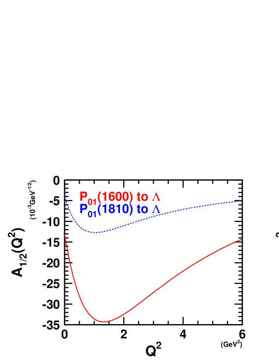
Figure 1: Helicity amplitudes $A_{1/2}$ and $C_{1/2}$ for the P₀₁(1600) (full line) and the P₀₁(1810) (dashed line) resonances.

References

• [1] R. M. Mohring et al., Phys. Rev. C67, 055205 (2003).
• [2] D. Merten et al., Eur. Phys. J. A14, 477 (2002).
• [3] U. Löring et al., Eur. Phys. J. A10, 309 (2001).
• [4] T. Van Cauteren et al., Eur. Phys. J. A20, 283 (2004).
• [5] M. I. Adamovich et al., Eur. Phys. J. C8, 59 (1999).
• [6] I. Eschrich et al. (SELEX Collaboration), Phys. Lett. B522 No.3-4, 233 (2001).
• [7] T. Hyodo et al., arXiV:nucl-th/0404031 (2004).