Does $\Sigma-\Sigma-\alpha$ Form a Quasi-Bound State?

Abstract

We have investigated the possible existence of a quasi-bound state for the $\Sigma-\Sigma-\alpha$ system in the framework of Faddeev calculations. We are particularly interested in the state of total iso-spin T=2, since for an inert $\alpha$ particle there is no strong conversion to $\Xi-N-\alpha$ or $\Lambda-\Lambda-\alpha$ possible. A $\Sigma-\alpha$ optical potential based on Nijmegen model D and original $\Sigma-\Sigma$ interactions of the series of Nijmegen potentials NSC97 as well a simulated Gaussian type versions thereof are used. Our investigation of the $\Sigma-\Sigma-\alpha$ system leads to a quasi bound state where, depending on the potential parameters, the energy ranges between -1.4 and -2.4 MeV and the level width is about 0.2MeV .

1 Introduction

Strangeness S=-2 hypernuclei provide information on baryon-baryon forces in the state of S=-2. Only three nuclei have been identified so far, ${}^{10}_{\Lambda\Lambda}Be$ [1], ${}^{6}_{\Lambda\Lambda}He$ [2] and ${}^{13}_{\Lambda\Lambda}B$ [3]. The challenge is to understand their binding energies and decay properties. These nuclei are especially interesting since the S=-2 two-baryon system is rich in structure due to the conversions between $\Lambda\Lambda$ , $\Xi N$ and $\Sigma\Sigma$. Baryon-baryon forces for S=0,-1 and -2 are being investigated in the meson exchange picture[4, 5, 6, 7] or using quark models[8]. While there is a wealth of data for S=0, which allows to fix force parameters, the situation is still much open in the S=-1 and -2 sectors. Therefore additional information is needed. In this study we would like to focus on the system $\Sigma-\Sigma-\alpha$ in the state of total iso-spin T=2. If the $\alpha$-particle would be inert, that system could not convert to $\Xi-N-\alpha$ or $\Lambda-\Lambda-\alpha$. Therefore in case the forces would be strong enough, there might exist a low lying state with a small width. The width would be caused by $\Lambda-\Sigma$ conversion leading , for instance, to $\Sigma+\Lambda+N+(^{3}He/^{3}H)$, where $(N+^{3}He/^{3}H)$ is in a state of total iso-spin T=1 or into $\Sigma+\Lambda+^{4}He^{*}$ (T=1).

We investigate that system $\Sigma-\Sigma-\alpha$ under effective simplifying assumptions. The $\Sigma-\alpha$ interaction is modeled via an optical potential based on the Nijmegen model D and the $\Sigma-\Sigma$ interaction in the state of total iso-spin T=2 is taken either directly as a meson theoretical Nijmegen potential of the type NSC97[6] or a simulated version thereof of the Gaussian type[9]. That 3-body system is solved precisely in the Faddeev scheme.

In section 2 we derive the Faddeev equations for the $\Sigma-\Sigma-\alpha$ system. The numerical results are displayed in section 3. The Appendix shows technical details of the formulation. We end with a brief summary of our work and an outlook in section 4.

2 The Faddeev Equations for the System $\Sigma-\Sigma-\alpha$

We assume the existence of a quasi-bound state where the width of that state is caused by the (absorptive) imaginary part of the effective $\Sigma-\alpha$ potential. If the $\alpha$ particle would be inert and the two $\Sigma$’s couple to iso-spin T=2, the system cannot convert into $\Xi-N-\alpha$ or $\Lambda-\Lambda-\alpha$. We focus on such a state with T=2. The Schrödinger equation reads

$$\left(H_{0}+V_{\Sigma\Sigma}+V_{\Sigma_{1}\alpha}+V_{\Sigma_{2}\alpha}\right)\Psi=E\Psi$$ (1)

It is convenient to number the two $\Sigma$’s as 1 and 2 and the $\alpha$ particle as 3. Then the Schrödinger equation converted into an integral equation reads

$$\Psi=\frac{1}{E-H_{0}}\left(V_{12}+V_{13}+V_{23}\right)\Psi$$ (2)

which suggests the decomposition

$$\Psi=\psi_{12}+\psi_{13}+\psi_{23}$$ (3)

with

$$\psi_{ij}=\frac{1}{E-H_{0}}V_{ij}\Psi$$ (4)

Because of the identity of the $\Sigma$’s and the antisymmetry of $\Psi$ the two Faddeev components $\psi_{23}$ and $\psi_{13}$ are not independent and are related to each other by

$$\psi_{13}=-P_{12}\psi_{23}$$ (5)

This then leads to two coupled equations

$$\psi_{12}=\frac{1}{E-H_{0}}V_{12}\left(\psi_{12}+\left(1-P_{12}\right)\psi_{23}\right)$$ (6)

$$\psi_{23}=\frac{1}{E-H_{0}}V_{23}\left(-P_{12}\psi_{23}+\psi_{12}\right)$$ (7)

In a standard manner one introduces the two-body t-matrices

$$t_{12}=V_{12}+V_{12}\frac{1}{E-H_{0}}t_{12}$$ (8)

$$t_{23}=V_{23}+V_{23}\frac{1}{E-H_{0}}t_{23}$$ (9)

and obtains the final set of two-coupled Faddeev equations

$$\psi_{12}=\frac{1}{E-H_{0}}t_{12}\left(1-P_{12}\right)\psi_{23}$$ (10)

$$\psi_{23}=\frac{1}{E-H_{0}}t_{23}\left(-P_{12}\psi_{23}+\psi_{12}\right)$$ (11)

The total state is then given as

$$\Psi=\left(1-P_{12}\right)\psi_{23}+\psi_{12}$$ (12)

We solve that system in momentum space and use a partial wave decomposition. To that aim we introduce two types of Jacobi momenta in terms of the individual momenta $\mathbf{k}_{i}$ , i=1,2,3;

$$\mathbf{p}_{3}=\frac{1}{2}\left(\mathbf{k}_{1}-\mathbf{k}_{2}\right)$$ (13)

$$\mathbf{q}_{3}=\frac{2m_{\Sigma}\mathbf{k}_{3}-m_{\alpha}\left(\mathbf{k}_{1}+\mathbf{k}_{2}\right)}{2m_{\Sigma}+m_{\alpha}}$$ (14)

and

$$\mathbf{p}_{1}=\frac{m_{\alpha}\mathbf{k}_{2}-m_{\Sigma}\mathbf{k}_{1}}{m_{\alpha}+m_{\Sigma}}$$ (15)

$$\mathbf{q}_{1}=\frac{\left(m_{\alpha}+m_{\Sigma}\right)\mathbf{k}_{1}-m_{\Sigma}\left(\mathbf{k}_{2}+\mathbf{k}_{3}\right)}{m_{\alpha}+2m_{\Sigma}}$$ (16)

The momenta $\mathbf{p}_{3}$ ,$\mathbf{q}_{3}$ and $\mathbf{p}_{1}$ ,$\mathbf{q}_{1}$ are adequate for the Faddeev amplitudes $\psi_{12}$ and $\psi_{23}$ which are driven by the two-body t-matrices $t_{12}$ and $t_{23}$, respectively. Related to these momenta are partial wave projected basis states

$$\left|p_{3}q_{3}\left(l_{3}s_{3}\right)j_{3}\lambda_{3}\left(j_{3}\lambda_{3}\right)JM(11)2\right\rangle\equiv\left|p_{3}q_{3}\alpha_{3}\right\rangle$$ (17)

and

$$\left|p_{1}q_{1}\left(l_{1}\frac{1}{2}\right)j_{1}\left(\lambda_{1}\frac{1}{2}\right)I_{1}\left(j_{1}I_{1}\right)JM(11)2\right\rangle\equiv\left|p_{1}q_{1}\alpha_{1}\right\rangle$$ (18)

The sequence of discrete quantum numbers denote orbital and spin angular momenta, their intermediate couplings and the couplings to the total 3-body angular momentum J with magnetic quantum number M. Finally (11)2 denotes the iso-spin coupling. Because of the identity of particles 1 and 2, $(l_{3}+s_{3})$ has to be even. This imposes the only restriction to these intermediate quantum numbers.

By a standard procedure[10] the coupled set of equations (10-11) is projected onto those basis states. It results

$$\psi^{\alpha_{3}}_{12}\left(p_{3}q_{3}\right) \equiv\left\langle p_{3}q_{3}\alpha_{3}\right.\left|\psi_{12}\right\rangle =\frac{2}{E-\frac{p^{2}_{3}}{2\mu_{3}}-\frac{q^{2}_{3}}{2M_{3}}}\sum_{\alpha_{1}}\int^{\infty}_{0}dq_{1}q^{2}_{1}$$ (19)

$$\int^{1}_{-1}dxt_{12}\left(p_{3},\pi_{2},E-\frac{q^{2}_{3}}{2M_{3}}\right)$$

$$G_{\alpha_{3}\alpha_{1}}\left(q_{3}q_{1}x\right)\psi^{\alpha_{2}}_{23}\left(\pi^{\prime}_{2,}q_{1}\right)$$

$$\psi^{\alpha_{1}}_{23}\left(p_{1}q_{1}\right) = \frac{1}{E-\frac{p^{2}_{1}}{2\mu_{1}}-\frac{q^{2}_{1}}{2M_{1}}}\sum_{\alpha_{3}}\int^{\infty}_{0}dq_{3}q^{2}_{3}\int^{1}_{-1}dxt_{23}\left(p_{1},\pi_{3},E-\frac{q^{2}_{1}}{2M_{1}}\right)$$ (20)

$$G_{\alpha_{3}\alpha_{1}}\left(q_{3}q_{1}x\right)\psi^{\alpha_{3}}_{12}\left(\pi^{\prime}_{3}q_{3}\right)$$

$$-\frac{1}{E-\frac{p^{2}_{1}}{2\mu_{1}}-\frac{q^{2}_{1}}{2M_{1}}}\sum_{\alpha^{\prime}_{1}}\int^{\infty}_{0}dq^{\prime}_{1}q^{\prime 2}_{1}\int^{1}_{-1}dxt_{23}\left(p_{1},\pi_{4},E-\frac{q^{2}_{1}}{2M_{1}}\right)$$

$$G_{\alpha_{1}\alpha^{\prime}_{1}}\left(q_{1}q^{\prime}_{1}x\right)\psi^{\alpha^{\prime}_{1}}_{23}\left(\pi^{\prime}_{4}q^{\prime}_{1}\right)$$

The purely geometrical quantities $G_{\alpha\alpha^{\prime}}$ resulting from recouplings are given in the Appendix. Further the shifted arguments in the two-body t-matrices and the Faddeev amplitudes under the integrals are given as

$\pi_{2}=\sqrt{q^{2}_{1}+\rho^{2}_{1}q^{2}_{3}+2\rho_{1}q_{1}q_{3}x}$        $\pi_{3}=\sqrt{\rho^{2}_{2}q^{2}_{1}+q^{2}_{3}+2\rho_{2}q_{1}q_{3}x}$

$\pi^{\prime}_{2}=\sqrt{\rho^{2}_{2}q^{2}_{1}+q^{2}_{3}+2\rho_{2}q_{1}q_{3}x}$         $\pi^{\prime}_{3}=\sqrt{q^{2}_{1}+\rho^{2}_{1}q^{2}_{3}+2\rho_{1}q_{1}q_{3}x}$

$\pi_{4}=\sqrt{\rho^{2}q^{2}_{1}+q^{\prime 2}_{1}+2\rho q_{1}q^{\prime}_{1}x}$         $\pi^{\prime}_{4}=\sqrt{q^{2}_{1}+\rho^{2}q^{\prime 2}_{1}+2\rho q_{1}q^{\prime}_{1}x}$

where $\rho_{1}=\frac{1}{2}$,$\rho_{2}=\frac{M_{\alpha}}{M_{\alpha}+M_{\Sigma}}$ and $\rho=\frac{M_{\Sigma}}{M_{\Sigma}+M_{\alpha}}$

The reduced masses are

$\mu_{3}=\frac{1}{2}M_{\Sigma}$

$M_{3}=\frac{2M_{\alpha}M_{\Sigma}}{2M_{\Sigma}+M_{\alpha}}$

$\mu_{1}=\frac{M_{\alpha}M_{\Sigma}}{M_{\alpha}+M_{\Sigma}}$

$M_{1}=\frac{M_{\Sigma}\left(M_{\Sigma}+M_{\alpha}\right)}{2M_{\Sigma}+M_{\alpha}}$

This is an infinite set of homogenous coupled integral equations in two variables, which can be truncated since the two-body t-matrices drop quickly in magnitude with increasing angular momenta.

3 Results

The set of coupled equations (19-20) are discretized in a standard manner. We choose Gaussian quadrature points in the variables q and x and spline interpolation for the variables $\pi$ under the integrals. The two-body t-matrices are generated from the Lippmann Schwinger equation again using Gaussian quadrature discretization. We refer for numerical details to [10, 11]. The energy eigenvalue E is determined as follows. The homogenous set of coupled equations is schematically written as

$$\eta(E)\psi=K(E)\psi$$

with $\eta(E)=1$ at the energy eigenvalue. Without knowing E, one first determines $\eta$ and varies E such that finally $\eta(E)=1$. The eigenvalue $\eta$ is determined either by a simple power method or by a Lanczos type algorithm. For details see [11, 12].

In order to demonstrate our numerical accuracy we would firstly like to display results on the $\Lambda\Lambda\alpha$ system, where for model forces we recalculated ${}^{6}_{\Lambda\Lambda}He$ binding energies. The model forces are of Gaussian types and we refer to [13, 14]. That system has been investigated before by Filikhin et al. [13] using Faddeev equations in configuration space and by Myint et al. [14] using a variational method based on a Gaussian expansion. Our method is mathematically different from theirs. We solved the Faddeev equations in momentum space which allows us to treat any type of two body forces. We show in Table 1 ${}^{6}_{\Lambda\Lambda}He$ binding energies for an increasing number of relative orbital angular momenta within the $\Lambda\alpha$ and $\Lambda\Lambda$ sub-systems. Our results are in very good agreement with the other two methods which underlines the reliability of our treatment.

$l_{\Lambda\alpha}$	$l_{\Lambda\Lambda}$	Ours	Filikhin	Myint
0	0	-6.880	-6.880	-6.880
0,1	0	-6.986	-6.987	-6.983
0,1,2	0,2	-7.050	-7.045	-7.041
0,1,2,3	0,2	-7.084	-7.078	-7.073

Table 1: Comparison of ${}^{6}_{\Lambda\Lambda}He$ binding energies in MeV based on the model forces given in [13] and [14] for an increasing number of partial waves.

Now we turn to the central topic, the $\Sigma\Sigma\alpha$ system in the state of total iso-spin T=2. For the $\Sigma-\Sigma$ potential we use either the original Nijmegen potentials NSC97a,c,e [4] or the simulated Gaussian forms thereof [9]. The latters are given as

$$V(r)=\sum^{2}_{i=1}V_{i}e^{-(r/\mu_{i})^{2}}$$ (21)

with the parameters shown in Table 2. The $\Sigma-\alpha$ potential is chosen to be complex to provide for absorptive processes, like the ones mentioned in the introduction. We use the form

$$V_{\Sigma\alpha}(r)=\sum^{2}_{i=1}V_{i}e^{-(r/\mu_{i})^{2}}+\sum^{2}_{i=1}U_{i}e^{-(r/\mu_{i})^{2}}$$ (22)

with the parameters $V_{1}=-21.3$ MeV, $V_{2}=4.8$ MeV for the real part and $U_{1}=4.07$ MeV, $U_{2}=-11.73$ MeV for the imaginary part. Further, one has $\mu_{1}=1.3$ fm and $\mu_{2}=1.7$ fm.

The $\Sigma-\alpha$ potential has been constructed in the following manner. An effective $\Sigma-N$ potential was firstly derived from the original Nijmegen model D interaction in the Brueckner framework. Then that effective potential was expanded into a five-range Gausian form. That potential was used in a generalized Hartree-Fock method to generate the effective $\Sigma-\alpha$ potential[15]. The imaginary part arises due to $\Lambda N$ to $\Sigma N$ conversion.

	$V_{1}$ (MeV)	$V_{2}$ (MeV)
NSC97a “sim”	5274.2576	-292.7193
NSC97c “sim”	4886.7830	-289.8740
NSC97e “sim”	4588.5040	-294.2548

Table 2: The potential strength parameters of the Gaussian form “sim” given in Eq.(21) for the $\Sigma-\Sigma$ system. The range parameters are $\mu_{1}=0.37$ fm and $\mu_{2}=1.0$ fm.

Figure 1: Energy trajectory in the complex energy plane for the $\Sigma-\alpha$ potential. The numbers at each point indicate the multiplicative factors by which the attractive real part and the over all imaginary parts were multiplied.

Before we present the result for the three-body system $\Sigma\Sigma\alpha$ we firstly investigate the properties of the underlying two-body sub-systems. The complex $\Sigma-\alpha$ potential leads to a complex energy eigenvalue. We locate the one with the “lowest” energy in the following manner. We neglect the imaginary part and multiply the attractive real part by some enhancement factor. Choosing for instance that factor to be 2.5 we find a binding energy of -1.0 MeV. Next we allow the imaginary part to increase from 0 in steps of 0.1 until we reach the physical value 1. In this manner we find the energy trajectory in the complex energy plane shown in Fig.1. We end up with the complex energy position in the lower energy half plane just below the unitarity cut from 0 to infinity. To reach that final position we have chosen that detour in the complex energy plane which appears to us more feasible than a direct energy search for the physical potential strength. Thus we find that the effective $\Sigma-\alpha$ potential is not strong enough to generate a complex energy with a negative real part. The energy search in the complex energy plane was greatly simplified by using a method of analytical continuation in the form of the point method [16].

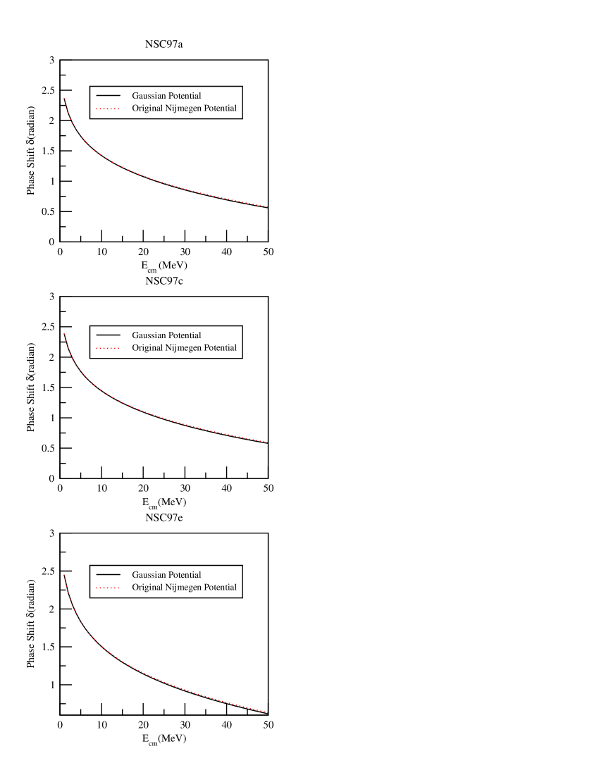
Figure 2: Comparison of $\Sigma\Sigma$-phase shifts for the original Nijmegen potentials NSC97a,c,e and the Gaussian potentials for ${}^{1}S_{0}$ $T=2$.

The chosen $\Sigma-\Sigma$ potentials support a bound state. The corresponding binding energies are displayed in Table 3 for the original Nijmegen potentials and the simulated ones. The phase shifts in the state ${}^{1}S_{0}$ and T=2 for the original and simulated potentials agree perfectly well with each other as shown in Fig.2. Though it is presumably unrealistic that two $\Sigma$’s are bound it is the result of the meson based Nijmegen potentials, whose parameters have been fixed to very many data in the nucleon-nucleon and hyperon-nucleon sectors and where SU(3) symmetry arguments allow for a prediction to the S=-2 sector. We shall comment below on an ad hoc weakening of those potentials.

	Gaussian	Nijmegen
NSC97a	-2.253	-2.250
NSC97c	-2.460	-2.437
NSC97e	-3.214	-3.122

Table 3: Comparison of the two-body $\Sigma\Sigma$ binding energies in MeV for the original Nijmegen potentials NSC97a,c,e and the simulated Gaussian potentials.

We are interested to see the outcome of those dynamical assumptions for the $\Sigma\Sigma\alpha$ system. In this exploratory investigation we restrict all orbital angular momenta to be zero. In the first step we neglect the imaginary part of the $\Sigma-\alpha$ potential. It turns out that in all cases using the original Nijmegen $\Sigma-\Sigma$ potentials or the simulated ones, the three-body system is bound. The results are given in Table 4. Then we switch on the imaginary part of the $\Sigma-\alpha$ potential in steps of 0.1. The results are displayed in Fig.3 and Fig.4 for the two cases. The effect of the imaginary part in the $\Sigma-\alpha$ potential shifts the real part of the energy slightly to the right and introduces a small negative imaginary part. The resulting final energy positions are displayed in Table 5.

Figure 3: Energy trajectories in the complex energy plane for the ${}^{6}_{\Sigma\Sigma}He$ system using the original $\Sigma-\Sigma$ Nijmegen NSC97e interaction. The numbers at each point indicate the multiplicative factors by which the attractive real part and the over all imaginary parts were multiplied.

Figure 4: Energy trajectories in the complex energy plane for the ${}^{6}_{\Sigma\Sigma}He$ system using the simulated Gaussian form for the $\Sigma-\Sigma$ Nijmegen NSC97e interaction. The numbers at each point indicate the multiplicative factors by which the attractive real part and the overall imaginary parts were multiplied.

	NSC97a	NSC97c	NSC97e
Nijmegen	-1.840	-2.378	-2.728
Gaussian	-1.841	-2.400	-2.819

Table 4: The energy eigen values in MeV for the $\Sigma\Sigma\alpha$ system using the simulated Gaussian and the original Nijmegen $\Sigma-\Sigma$ potentials together with the real part alone of the $\Sigma-\alpha$ potential.

	NSC97a	NSC97c	NSC97e
Nijmegen	-1.418- i0.202	-2.34- i0.014	-2.376- i0.191
Gaussian	-1.492- i0.218	-2.323- i0.017	-2.354- i0.211

Table 5: The complex energy eigen values in MeV for the $\Sigma\Sigma\alpha$ system using the simulated Gaussian and the original Nijmegen $\Sigma-\Sigma$ potentials together with the complex $\Sigma-\alpha$ potentials.

In order to explore the outcome using $\Sigma-\Sigma$ potentials which are weaker than the ones we used, we multiplied them by overall factors 0.9 and 0.8. The resulting $\Sigma-\Sigma$ binding energies for the original NSC97e potential are -1.5 and -0.4 MeV, respectively ( in comparison to the original value of -3.1 MeV). Then we performed again the energy search for the $\Sigma-\Sigma-\alpha$ system starting with zero imaginary part for the effective $\Sigma-\alpha$ potential. In case of the reduction factor 0.9 (0.8) this leads to a 3-body binding energy of -1.08 MeV (-0.32 MeV). For the full imaginary part we end up with (0.68 - i 0.21) MeV for the factor 0.9 and with(-0.279 - i 2.0$\times$ $10^{-2}$ ) MeV for the factor 0.8. We conjecture that a low lying quasi bound state or a resonance for the $\Sigma-\Sigma-\alpha$ system in the T=2 might exist in reality.

Finally we would like to mention a possible means to approach such a state experimentally. One could think of the two step process of $(K^{-},K^{+})$ reaction on a ${}^{6}Li$ target;

$K^{-}+^{6}Li\rightarrow\Sigma^{0}+\pi^{0}+n+^{4}_{2}He$

$\pi^{0}+n\rightarrow\Sigma^{-}+K^{+}$

In this manner one populates two $\Sigma$’s together with $\alpha$. It remains of course the task to estimate the reaction rates.

4 Summary and Outlook

We developed a Faddeev code for the effective three-body systems $\Lambda\Lambda\alpha$ and $\Sigma\Sigma\alpha$. It is formulated in momentum space and is applicable for any type of two-baryon forces. This allowed us to use directly the original Nijmegen forces, which is the first time, to the best of our knowledge, that they have been applied for these systems. We tested our code in a bench mark model study for the $\Lambda\Lambda\alpha$ system reproducing perfectly well the results from two earlier studies. Our results for the $\Sigma\Sigma\alpha$ system lead to a quasi bound state with a small negative imaginary part. The negative real part of the energy ranges between -1.4 and -2.4 MeV. These numbers are based on the original or simulated Nijmegen potentials for the $\Sigma\Sigma$ system in the state T=2, which support a bound state with a binding energy of about -2.5 MeV. Further we use a $\Sigma-\alpha$ optical model potential, which by itself supports a complex energy eigen value of about (-2 -i 0.1) MeV. We also artificially reduced the overall strength of the $\Sigma-\Sigma$ potential by factors 0.9 and 0.8, which moved the 3-body $\Sigma-\Sigma-\alpha$ energies towards -0.68 and -0.279 MeV, respectively,with small widths.

Both dynamical assumptions on the $\Sigma-\Sigma$ and $\Sigma-\alpha$ potentials should be critically reinvestigated in the future. Upcoming meson based $\Sigma-\Sigma$ potentials without a bound state should be used and in addition the effective $\Sigma-\alpha$ potential should be generated more consistently using realistic $\alpha$ particle wave functions in conjunction with $\Sigma$-nucleon forces related to the same theoretical model as for the $\Sigma-\Sigma$ interaction. A low lying state for the $\Sigma-\Sigma-\alpha$ system with isospin T=2 would provide interesting additional information on the dynamics in the strangeness S=-2 sector.

Appendix

The purely geometrical coefficients occuring in Eqs(19) and (20) are

$$\mathcal{G}_{\alpha_{3}\alpha^{\prime}_{1}}\left(q_{3},q^{\prime}_{1},x\right)$$ (23)

$$= \frac{1}{4}(-)^{j+\lambda+1+l^{\prime}}\sqrt{\hat{j}\,\hat{j}^{\prime}\,\hat{I}^{\prime}\,\hat{s}\,\hat{l}\,\hat{\lambda}\,\hat{l}^{\prime}\,\hat{\lambda}^{\prime}}\,\sum_{Ls}\hat{L}(-)^{L}\left\{\begin{array}[]{ccc}s&l&j\\ \lambda&J&L\end{array}\right\}\left\{\begin{array}[]{ccc}l^{\prime}&\frac{1}{2}&j^{\prime}\\ \lambda^{\prime}&\frac{1}{2}&I^{\prime}\\ L&s&J\end{array}\right\}$$ (38)

$$\sum_{l_{1}+l_{2}=l}\,\sum_{l^{\prime}_{1}+l^{\prime}_{2}=l^{\prime}}\rho^{l_{2}}_{1}\,\rho^{l^{\prime}_{1}}_{2}\,\left(q_{3}\right)^{l_{2}+l^{\prime}_{2}}\,\left(q^{\prime}_{1}\right)^{l^{\prime}_{1}+l_{1}}$$

$$\sqrt{\frac{\left(2l+1\right)!}{2l_{1}!2l_{2}!}}\,\sqrt{\frac{\left(2l^{\prime}+1\right)!}{2l^{\prime}_{1}!2l^{\prime}_{2}!}}\,\sum_{f}\left\{\begin{array}[]{ccc}l_{1}&l_{2}&l\\ \lambda&L&f\end{array}\right\}C\left(l_{2}\lambda f;00\right)$$

$$\sum_{f^{\prime}}\left\{\begin{array}[]{ccc}l^{\prime}_{2}&l^{\prime}_{1}&l^{\prime}\\ \lambda^{\prime}&L^{\prime}&f^{\prime}\end{array}\right\}C\left(l^{\prime}_{1}\lambda^{\prime}f^{\prime};00\right)\sum_{k}\,\hat{k}\,P_{k}(x)\,\sum_{h}\,\hat{h}\,g_{h}\sum_{f^{\prime\prime}}\,C\left(khf^{\prime\prime};00\right)^{2}$$

$$\left\{\begin{array}[]{ccc}f&l_{1}&L\\ f^{\prime}&l^{\prime}_{2}&f^{\prime\prime}\end{array}\right\}C\left(f^{\prime\prime}l^{\prime}_{2}f;00\right)C\left(f^{\prime\prime}l_{1}f^{\prime};00\right)$$

with

$$g_{h}=\int^{1}_{-1}dxP_{h}(x)\frac{1}{\left|\rho_{2}\mathbf{q}^{\prime}_{1}+\mathbf{q}_{3}\right|^{l^{\prime}}}\frac{1}{\left|\mathbf{q}^{\prime}_{1}+\rho_{1}\mathbf{q}_{3}\right|^{l}}$$

and

$$\mathcal{G}_{\alpha_{1}\alpha^{\prime}_{1}}\left(q_{1},q^{\prime}_{1},x\right)$$ (39)

$$= \frac{1}{4}\sum_{LS}\,(-)^{1-S}\sqrt{\hat{j}\,\hat{I}\,\hat{j}^{\prime}\,\hat{I}^{\prime}\hat{l}\,\hat{\lambda}\hat{l}^{\prime}\,\hat{\lambda}^{\prime}}\,\,\hat{L}\,\hat{S}\left\{\begin{array}[]{ccc}l&\frac{1}{2}&j\\ \lambda&\frac{1}{2}&I\\ L&S&J\end{array}\right\}\left\{\begin{array}[]{ccc}l^{\prime}&\frac{1}{2}&j^{\prime}\\ \lambda^{\prime}&\frac{1}{2}&I^{\prime}\\ L&S&J\end{array}\right\}$$ (55)

$$\sum_{l_{1}+l_{2}=l}\,\sum_{l^{\prime}_{1}+l^{\prime}_{2}=l^{\prime}}\,\rho^{l^{\prime}_{1}+l_{2}}\,\,\left(q^{\prime}_{1}\right)^{l_{1}+l^{\prime}_{1}}\,\left(q_{1}\right)^{l_{2}+l^{\prime}_{2}}$$

$$\sqrt{\frac{\left(2l+1\right)!}{2l_{1}!2l_{2}!}}\,\sqrt{\frac{\left(2l^{\prime}+1\right)!}{2l^{\prime}_{1}!2l^{\prime}_{2}!}}\,\sum_{f}\left\{\begin{array}[]{ccc}l_{1}&l_{2}&l\\ \lambda&L&f\end{array}\right\}C\left(l_{2}\lambda f;00\right)$$

$$\sum_{f^{\prime}}\left\{\begin{array}[]{ccc}l^{\prime}_{2}&l^{\prime}_{1}&l^{\prime}\\ \lambda^{\prime}&L&f^{\prime}\end{array}\right\}C\left(l^{\prime}_{1}\lambda^{\prime}f^{\prime};00\right)\sum_{k}\hat{k}P_{k}(x)\,\sum_{h}\,\hat{h}g_{h}$$

$$\sum_{f^{\prime\prime}}\,C\left(khf^{\prime\prime};00\right)^{2}\left\{\begin{array}[]{ccc}f&l_{1}&L\\ f^{\prime}&l^{\prime}_{2}&f^{\prime\prime}\end{array}\right\}C\left(f^{\prime\prime}l^{\prime}_{2}f;00\right)C\left(f^{\prime\prime}l_{1}f^{\prime};00\right)$$

with

$$g_{h}=\int^{1}_{-1}dxP_{h}(x)\frac{1}{\left|\rho\mathbf{q}_{1}+\mathbf{q}^{\prime}_{1}\right|^{l}}\frac{1}{\left|\mathbf{q}_{1}+\rho\mathbf{q}^{\prime}_{1}\right|^{l^{\prime}}}$$

References

• [1] M. Danysz et al., \NPA49,1963,121
• [2] D.J. Prowse, \PRL17,1966,782
• [3] S. Aoki et al., \PTP85,1991,1287
• [4] Th.A. Rijken,V.G.J. Stoks and Y. Yamamoto, \PRC59,1999,21
• [5] V.G.J.Stoks and Y.Yamamoto, \PRC59,1999,3009
• [6] Th.A. Rijken, \NPA691,2001,322c
• [7] A. Reuber,K. Holinde and J. Speth, \NPA570,1990,543
• [8] Y. Fujiwara, C. Nakamoto and Y. Suzuki, \PRC54,1996,2180
• [9] Y. Akaishi and S. Shinmura, private communication
• [10] W.GlΓΆckle, The Quantum Mechanical Few-Body Problem, Springer Verlag, (1983)
• [11] Htun Htun Oo’s doctoral thesis, 2004, Mandalay University, unpublished
• [12] A. Stadler, W. GlΓΆckle, and P.U. Sauer, \PRC44,1991,2319
• [13] I.N. Filikhin, A. Gal, and V.M. Suslov, nucl-th/0303028
• [14] Khin Swe Myint, S. Shinmura and Y. Akaishi, Eur. Phys. J. A16 (2003), 21
• [15] Y. Akaishi, Private communication
• [16] L. Schlessinger, Phys.Β Rev.Β 167 (1986), 1411