Models of Meson-Baryon Reactions in the Nucleon Resonance Region

Abstract

It is shown that most of the models for analyzing meson-baryon reactions in the nucleon resonance region can be derived from a Hamiltonian formulation of the problem. An extension of the coupled-channel approach to include $\pi\pi N$ channel is briefly described and some preliminary results for the $N^{*}(1535)$ excitation are presented.

1 Introduction

With very successful experimental efforts in the past few years, we are now facing a challenge to interpret very extensive data of electromagnetic meson production reactions in terms of the structure of nucleon resonances ($N^{*}$). To achieve this goal, we need to perform amplitude analyses of the data in order to extract $N^{*}$ parameters. We also need to develop reaction models to analyze the dynamical content of the extracted $N^{*}$ parameters. At the present time, we can use the $N^{*}$ data to test the predictions from various QCD-based hadron models. In the near future, we hope to understand $N^{*}$ parameters from Lattice QCD.

In the $\Delta$ region, both the amplitude analyses and dynamical reaction models have been well developed. We find that these two efforts are complementary. For example, the $\gamma N\rightarrow\Delta$ M1 transition strength extracted from all amplitude analyses is $G_{M}(0)=3.18\pm 0.04$ which is about 40 $\%$ larger than the constituent quark model prediction. This difference is understood[1, 2] by developing dynamical reaction models within which one can show that the discrepancy is due to the pion cloud which is not included in the commonly considered constituent quark model prediction.

In the second and third resonance regions, the situation is much more complicated because of many open channels. It is necessary to develop coupled-channel approaches for learning about the $N^{*}$ properties. The main objective of this contribution is to review the development in this direction. We will also describe a newly developed coupled-channel model which is aimed at accounting for rigorously the $\pi\pi N$ unitarity condition.

In section 2, we will introduce a Hamiltonian formulation within which most of the current models of electromagnetic meson production reactions can be derived and compared. The extension of the coupled-channel approach to account for explicitly the $\pi\pi N$ channel is then described in section 3. A summary is given in section 4.

2 Derivation of Models

The starting point of our derivation is to assume that the meson-baryon ($MB)$ reactions can be described by a Hamiltonian of the following form

$$H=H_{0}+V\,,$$ (1)

where $H_{0}$ is the free Hamiltonian and

$$V=v^{bg}+v^{R}\,.$$ (2)

Here $v^{bg}$ is the non-resonant(background) term due to the mechanisms such as the tree-diagram mechanisms illustrated in Fig. 1(a)-(d), and $v^{R}$ describes the $N^{*}$ excitation Fig. 1(e). Schematically, the resonant term can be written as

$$v^{R}(E)=\sum_{N^{*}_{i}}\frac{\Gamma^{\dagger}_{i}\Gamma_{i}}{E-M^{0}_{i}}\,,$$ (3)

where $\Gamma_{i}$ defines the decay of the $i$-th $N^{*}$ state into meson-baryon states, and $M^{0}_{i}$ is a mass parameter related to the resonance position.

Figure 1: Tree diagrams for meson-baryon reactions. $N^{*}$ is a nucleon resonance state.

The next step is to define a channel space spanned by the considered meson-baryon ($MB$) channels: $\gamma N$, $\pi N$, $\eta N$, $\pi\Delta$, $\rho N$ $\sigma N$, $\cdot\cdot$. The S-matrix of the meson-baryon reaction is defined by

$$S(E)_{a,b}=\delta_{a,b}-2\pi i\delta(E-H_{0})T_{a,b}(E)\,,$$ (4)

where ($a,b$) denote $MB$ channels, and the scattering T-matrix is defined by the following coupled-channel equation

$$T_{a,b}(E)=V_{a,b}+\sum_{c}V_{a,c}g_{c}(E)T_{c,b}(E)\,.$$ (5)

Here the meson-baryon propagator of channel $c$ is

$$g_{c}(E)=<c\mid g(E)\mid c>$$

with

$$g(E) = \frac{1}{E-H_{0}+i\epsilon}\,$$ (6)

$$= g^{P}(E)-i\pi\delta(E-H_{0})\,,$$

where

$$g^{P}(E) = \frac{P}{E-H_{0}}\,.$$ (7)

Here $P$ denotes taking the principal-value part of any integration over the propagator. If $g(E)$ in Eq.(5) is replaced by $g^{P}(E)$, we then define the K-matrix which is related to T-matrix by

$$T_{a,b}(E)=K_{a,b}(E)-\sum_{c}T_{a,c}(E)[i\pi\delta(E-H_{0})]_{c}K_{c,b}(E)\,.$$ (8)

By using the two potential formulation, one can cast Eq.(5) into

$$T_{a,b}(E) = t^{bg}_{a,b}(E)+t^{R}_{a,b}(E)$$ (9)

with

$$t^{R}_{a,b}(E) = \sum_{N^{*}_{i},N^{*}_{j}}\bar{\Gamma}^{\dagger}_{N^{*}_{i},a}(E)[G(E)]_{i,j}\bar{\Gamma}_{N^{*}_{j},b}(E)\,.$$ (10)

The first term of Eq.(9) is determined only by the non-resonant interaction

$$t^{bg}_{a,b}(E)=v^{bg}_{a,b}+\sum_{c}v^{bg}_{a,c}g_{c}(E)t^{bg}_{c,b}(E)\,.$$ (11)

The resonant amplitude Eq.(10) is determined by the dressed vertex

$$\bar{\Gamma}_{N^{*},a}(E) = {\Gamma_{N^{*},a}}+\sum_{b}\Gamma_{N^{*},b}g_{b}(E)t^{bg}_{b,a}(E)\,,$$ (12)

and the dressed propagator

$$[G(E)^{-1}]_{i,j}(E)=(E-M^{0}_{N^{*}_{i}})\delta_{i,j}-\Sigma_{i,j}(E)\,.$$ (13)

Here $M_{N^{*}}^{0}$ is the bare mass of the resonance state $N^{*}$, and the self-energy is

$$\Sigma_{i,j}(E)=\sum_{a}\Gamma^{\dagger}_{N^{*},a}g_{a}(E)\bar{\Gamma}_{N^{*}_{j},a}(E)\,.$$ (14)

Note that the meson-baryon propagator $g_{a}(E)$ for channels including an unstable particle, such as $\pi\Delta$, $\rho N$ and $\sigma N$, must be modified to include a width. In the Hamiltonian formulation, this amounts to the following replacement

$$g_{a}(E)\rightarrow<a\mid\frac{1}{E-H_{0}-\Sigma_{V}(E)}\mid a>\,,$$ (15)

where the energy shift is

$$\Sigma_{V}(E)=\sum_{i}\Gamma^{+}_{V}(i)\frac{P_{\pi\pi N}}{E-H_{0}+i\epsilon}\Gamma_{V}(i)\,.$$ (16)

Here $\Gamma_{V}$ describes the decay of $\rho$, $\sigma$ or $\Delta$ in the quasi-particle channels.

Eq.(5), Eqs.(9)-(16), and Eq.(8) are the starting points of our derivations. From now on, we consider the formulation in the partial-wave representation. The channel labels, ($a,b,c$), will also include the usual angular momentum and isospin quantum numbers.

2.1 Unitary Isobar Model ($UIM$)

2.1.1 MAID

The Unitary Isobar Model developed[3] by the Mainz group is based on the on-shell relation Eq.(8). By including only one hadron channel, $\pi N$ (or $\eta N$ ), Eq.(8) leads to

$$T_{\pi N,\gamma N}=e^{i\delta_{\pi N}}cos\delta_{\pi N}K_{\pi N,\gamma N}\,.$$ (17)

where $\delta_{\pi N}$ is the pion-nucleon scattering phase shift. By further assuming that $K=V=v^{bg}+v^{R}$, one can cast the above equation into the following form

$$T_{\pi N,\gamma N}({\it UIM})=e^{\delta_{\pi N}}cos\delta_{\pi N}[v^{bg}_{\pi N,\gamma N}]+\sum_{N^{*}_{i}}T^{N^{*}_{i}}_{\pi N,\gamma N}(E)\,.$$ (18)

The non-resonant term $v^{bg}$ in Eq.(18) is calculated from the standard Born terms but with an energy-dependent mixture of pseudo-vector (PV) and pseudo-scalar (PS) $\pi NN$ coupling and the $\rho$ and $\omega$ exchanges. For resonant terms in Eq.(18), MAID uses the following Walker’s parameterization[5]

$$T^{N^{*}_{i}}_{\pi N,\gamma N}(E)=f^{i}_{\pi N}(E)\frac{\Gamma_{tot}M_{i}e^{i\Phi}}{M^{2}_{i}-E^{2}-iM_{i}\Gamma^{tot}}f^{i}_{\gamma N}(E)\bar{A}^{i}\,,$$ (19)

where $f^{i}_{\pi N}(E)$ and $f^{i}_{\gamma N}(E)$ are the form factors describing the decays of $N^{*}$, $\Gamma_{tot}$ is the total decay width, $\bar{A}^{i}$ is the $\gamma N\rightarrow N^{*}$ excitation strength. The phase $\Phi$ is required by the unitary condition and is determined by an assumption relating the phase of the total production amplitude to the $\pi N$ phase shift and inelasticity.

2.1.2 JLab/Yeveran UIM

The Jlab/Yerevan UIM[4] is similar to MAID. But it implements the Regge parameterization in calculating the amplitudes at high energies. It also uses a different procedure to unitarize the amplitudes.

Both MAID and JLab/Yeveran UIM have been applied extensively to analyze the data of $\pi$ and $\eta$ production reactions. Very useful new information on $N^{*}$ have been extracted.

2.2 Multi-channel K-matrix models

2.2.1 SAID

The model employed in SAID[6] is based on the on-shell relation Eq.(8) with three channels: $\gamma N$, $\pi N$, and $\pi\Delta$ which represents all other open channels. The solution of the resulting $3\times 3$ matrix equation can be written as

$$T_{\gamma N,\pi N}(SAID)=A_{I}(1+iT_{\pi N,\pi N})+A_{R}T_{\pi N,\pi N}\,,$$ (20)

where

$$A_{I} = K_{\gamma N,\pi N}-\frac{K_{\gamma N,\pi\Delta}K_{\pi N,\pi N}}{K_{\pi N,\pi\Delta}}\,,$$ (21)

$$A_{R} = \frac{K_{\gamma N,\pi\Delta}}{K_{\pi N,\pi\Delta}}\,.$$ (22)

In actual analysis, they simply parameterize $A_{I}$ and $A_{R}$ as

$$A_{I} = [v_{\gamma N,\pi N}^{bg}]+\sum_{n=0}^{M}\bar{p}_{n}zQ_{l_{\alpha}+n}(z)\,,$$ (23)

$$A_{R} = \frac{m_{\pi}}{k_{0}}(\frac{q_{0}}{k_{0}})^{l_{\alpha}}\sum_{n=0}^{N}p_{n}(\frac{E_{\pi}}{m_{\pi}})^{n}\,,$$ (24)

where $k_{0}$ and $q_{0}$ are the on-shell momenta for pion and photon respectively, $z=\sqrt{k^{2}_{0}+4m_{\pi}^{2}}/k_{0}$, $Q_{L}(z)$ is the legendre polynomial of second kind, $E_{\pi}=E_{\gamma}-m_{\pi}(1+m_{\pi}/(2m_{N}))$, and $p_{n}$ and $\bar{p}_{n}$ are free parameters. SAID calculates $v^{bg}_{\gamma N,\pi N}$ of Eq.(23) from the standard PS Born term and $\rho$ and $\omega$ exchanges. The empirical $\pi N$ amplitude $T_{\pi N,\pi N}$ needed to evaluate Eq.(20) is also available in SAID.

Once the parameters $\bar{p}_{n}$ and $p_{n}$ in Eqs.(23)-(24) are determined, the $N^{*}$ parameters are then extracted by fitting the resulting amplitude $T_{\gamma N,\pi N}$ at energies near the resonance position to a Breit-Wigner parameterization(similar to Eq.(19)). Very extensive data of pion photoproduction have been analyzed by SAID. The extension of SAID to also analyze pion electroproduction data is being pursued.

2.2.2 Giessen Model

The coupled-channel model developed by the Giessen group [7] can be obtained from Eq.(8) by taking the approximation $K=V$. This leads to a matrix equation involving only the on-shell matrix elements of $V$

$$T_{a,b}({\it Giessen})=\sum_{c}[(1+iV(E))^{-1}]_{a,c}V_{c,b}(E)\,.$$ (25)

The interaction $V=v^{bg}+v^{R}$ is evaluated from tree-diagrams of various effective lagrangians. The form factors, coupling constants, and resonance parameters are adjusted to fit both the $\pi N$ and $\gamma N$ reaction data. They include up to 5 channels in some fits, and have identified several new $N^{*}$ states. But further confirmations are needed to establish their findings conclusively.

2.2.3 KSU Model

The Kent State University (KSU) model[8] can be derived by noting that the non-resonant amplitude $t^{bg}$, defined by a $hermitian$ $v^{bg}$ in Eq.(11), define a S-matrix with the following properties

$$S^{bg}_{a,b}(E) = \delta_{a,b}-2\pi i\delta(E-H_{0})t^{bg}_{a,b}(E)$$ (26)

$$= \sum_{c}\omega^{(+)T}_{a,c}(E)\omega^{(+)}_{c,b}(E)\,,$$ (27)

where the non-resonant scattering operator is

$$\omega^{(+)}_{a,c}(E) = \delta_{a,c}+g_{a}(E)t^{bg}_{a,c}(E)\,.$$ (28)

With some derivations, the S-matrix Eq.(4) and the scattering T-matrix defined by Eqs.(9)-(14) can then be cast into following form

$$S_{a,b}(E)=\sum_{c,d}\omega^{(+)T}_{a,c}(E)R_{c,d}(E)\omega^{(+)}_{c,b}(E)\,,$$ (29)

with

$$R_{c,d}(E)=\delta_{c,d}+2iT^{R}_{c,d}(E)\,.$$ (30)

Here we have defined

$$T^{R}_{c,d}(E)=\sum_{i,j}\Gamma^{\dagger}_{N^{*}_{i},c}(E)[G(E)_{i,j}{\Gamma}_{N^{*}_{j},d}(E)\,.$$ (32)

The above set of equations is identical to that used in the KSU model of Ref.[8]. In practice, the KSU model fits the data by parameterizing $T^{R}$ as a Breit-Wigner resonant form $T^{R}\sim x\Gamma/2/(E-M-i\Gamma/2)$ and setting $\omega^{(+)}=B=B_{1}B_{2}\cdot\cdot\cdot B_{n}$, where $B_{i}=exp(iX\Delta_{i})$ is a unitary matrix.

The KSU model has been applied to $\pi N$ reactions, including pion photoproduction. It is now being extended to investigate $\bar{K}N$ reactions.

2.3 The CMB Model

A unitary multi-channel isobar model with analyticity was developed[9] in 1970’s by the Carnegie-Mellon Berkeley(CMB) collaboration for analyzing the $\pi N$ data. The CMB model can be derived by assuming that the non-resonant potential $v^{bg}$ is also of the separable form of $v^{R}$ of Eq.(3)

$$v^{bg}_{a,b}=\frac{\Gamma^{\dagger}_{L,a}\Gamma_{L,b}}{E-M_{L}}+\frac{\Gamma^{\dagger}_{H,a}\Gamma_{H,b}}{E-M_{H}}$$ (33)

The resulting coupled-channel equations are identical to Eqs.(9)-(16), except that $t^{bg}_{a,b}=0$ and the sum over $N^{*}_{i}$ is now extended to include these two distance poles $L$ and $H$.

By changing the integration variables and adding a substraction term, Eq.(14) can lead to CMB’s dispersion relations

$$\Sigma_{i,j}(s) = \sum_{c}\gamma_{i,c}\Phi_{c}(s)\gamma_{j,c}\,,$$ (34)

$$Re[\Phi_{c}(s)] = Re[\Phi_{c}(s_{0})]+\frac{s-s_{th,c}}{\pi}\int_{s_{th}}^{\infty}\frac{Im[\Phi_{c}(s^{\prime})]}{(s^{\prime}-s)(s^{\prime}-s_{0})}ds^{\prime}\,.$$ (35)

Thus CMB model is analytic in structure which marks its difference with all K-matrix models described above.

The CMB model has been revived in recent years by the Zagreb group[10] and a Pittsburgh-ANL collaboration[11] to extract the $N^{*}$ parameters from fitting the recent empirical $\pi N$ and $\gamma N$ reaction amplitudes. The resulting $N^{*}$ parameters have very significant differences with what are listed by PDG in some partial waves. In particular, several important issues concerning the extraction of the $N^{*}$ parameters in $S_{11}$ channel have been analyzed in detail.

2.4 Dynamical Models

A. In the $\Delta$ region

Keeping only one resonance $N^{*}=\Delta$ and two channels $a,b=\pi N,\gamma N$, Eqs.(9)-(14) are reduced to what were developed in the Sato-Lee (SL) model[1]. In solving exactly Eqs.(9)-(14), the non-resonant interactions $v^{bg}_{\pi N,\pi N}$ and $v^{bg}_{\pi N,\gamma N}$ are derived from the standard PV Born terms and $\rho$ and $\omega$ exchanges by using an unitary transformation method.

In the Dubna-Mainz-Taiwan (DMT) model[2], they depart from the formulation Eqs.(9)-(14) by using the Walker’s parameterization defined by Eq.(19) to describe the resonant term $t^{R}$ of Eq.(9). Accordingly, their definition of the non-resonant amplitude also differs from Eq.(11): $t^{bg}_{c,b}$ in the right-hand side of Eq.(11) is replaced by the full amplitude $T_{c,b}$. Furthermore, they follow MAID to calculate the non-resonant interaction $v^{bg}_{\pi N,\gamma N}$ from an energy-dependent mixture of PS and PV Born terms.

Extensive data of pion photoproduction and electroproduction in the $\Delta$ region can be described by both the SL and DMT models. However, the extracted $\gamma N\rightarrow\Delta$ form factors, in particular their bare form factors, are significantly different.

B. In the second and third resonance regions

Eqs.(9)-(16) are used in a 2-$N^{*}$ and 3-channel ($\pi N$, $\eta N$, and $\pi\Delta$) study[12] of $\pi N$ scattering in $S_{11}$ partial wave, aiming at investigating how the quark-quark interaction in the constituent quark model can be determined directly by using the reaction data. Eqs.(9)-(16) are also the basis of examining the $N^{*}$ effects[13] and one-loop coupled-channel effects[14] on $\omega$ meson photoproduction and the coupled-channel effects on $K$ photoproduction[15].

The coupled-channel study of both $\pi N$ scattering and $\gamma N\rightarrow\pi N$ in $S_{11}$ channel by Chen et al[16] includes $\pi N$, $\eta N$, and $\gamma N$ channels. Their $\pi N$ scattering calculation is performed by using Eq.(5), which is of course equivalent to Eqs.(9)-(14). In their $\gamma N\rightarrow\pi N$ calculation, they neglect the $\gamma N\rightarrow\eta N\rightarrow\pi N$ coupled-channel effect, and follow the procedure of the DMT model to evaluate the resonant term in terms of the Walker’s parameterization (Eq.(19)). They find that four $N^{*}$ are needed to fit the empirical amplitudes in $S_{11}$ channel up to $W=2$ GeV.

A coupled-channel calculation based on Eq.(5) has been carried out by Jülich group[17] for $\pi N$ scattering. They are able to describe the $\pi N$ phase shifts up to $W=1.9$ GeV by including $\pi N$, $\eta N$, $\pi\Delta$, $\rho N$ and $\sigma N$ channels and 5 $N^{*}$ resonances : $P_{33}(1232)$, $S_{11}(1535)$, $S_{11}(1530)$, $S_{11}(1650)$ and $D_{13}(1520)$. They find that the Roper resonance $P_{11}(1440)$ is completely due to the meson-exchange coupled-channel effects.

A coupled channel calculation based on Eq.(5) for both $\pi N$ scattering and $\gamma N\rightarrow\pi N$ up to $W=1.5$ GeV has been reported by Fuda and Alarbi[18]. They include $\pi N$, $\gamma N$, $\eta N$, and $\pi\Delta$ channels and 4 $N^{*}$ resonances : $P_{33}(1232)$, $P_{11}(1440)$, $S_{11}(1535)$, and $D_{13}(1520)$. The parameters are adjusted to fit the empirical multipole amplitudes in a few low partial waves.

Much simpler coupled-channel calculations have been performed by using separable interactions. In the model of Gross and Surya[19], such separable interactions are from simplifying the meson-exchange mechanisms in Figs 1.(a)-c) as a contact term like Fig. 1(d). They include only $\pi N$ and $\gamma N$ channels and 3 resonances: $P_{33}(1232)$, $P_{11}(1440)$ and $D_{13}(1520)$, and restrict their investigation up to $W<1.5$ GeV. To account for the inelasticities in $P_{11}$ and $D_{13}$, the $N^{*}\rightarrow\pi\Delta$ coupling is introduced in these two partial waves. The inelasticities in other partial waves are neglected.

A similar separable simplification is also used in the chiral coupled-channel models[20, 21] for strange particle production. There the separable interactions are directly determined from the leading contact terms of SU(3) effective chiral lagrangian and hence only act on s-wave partial waves. They are able to fit the total cross section data for various strange particle production reaction channels without introducing resonance states. It remains to be seen whether these models can be further improved to account for higher partial waves which are definitely needed to give an accurate description of the data even at energies near production thresholds.

Figure 2:

3 Unitary $\pi\pi N$ Model

All of the models described in section 2 rely on the assumption that the $\pi\pi N$ $continuum$ can be expanded in terms of quasi-two-particle channels such as $\pi\Delta$, $\sigma N$ , and $\rho N$. These models are of course not satisfactory since they do not account for all of the effects due to the coupling with the $\pi\pi N$ channel. It is necessary to develop a reaction model which also satisfies the $\pi\pi N$ unitarity condition exactly, This can be done by extending the Hamiltonian Eqs.(1)-(3) to include a vertex interaction $\Gamma_{V}$ to account for the $\rho\rightarrow\pi\pi$ and $\sigma\rightarrow\pi\pi$ decays and to include possible non-resonant $\pi\pi$ interaction $v_{\pi\pi}$. Such a formulation and numerical methods for performing unitary calculations of two-pion production cross sections are being pursued by Lee, Matsuyama, and Sato (LMS)[22]. Here we only briefly describe this unitary $\pi\pi N$ model.

The coupled-channel equations from LMS can also be cast into the form of Eqs.(9)-(16) except that the driving term of Eq.(11) is replaced by

$$v^{bg}_{a,b}\rightarrow\hat{V}_{a,b}=v^{bg}_{a,b}+X_{a,b}(E)$$ (36)

with

$$X_{a,b}(X)=Z_{a,b}(E)+\sum_{c}Z_{a,c}(E)g_{c}(E)X_{c,b}(E)\,.$$ (37)

The driving term of the above integral equation is

$$Z_{a,b}(E) = \sum_{i\neq j}<a\mid\Gamma_{V}^{+}(i)\frac{P_{\pi\pi N}}{E-H_{0}-v_{\pi N,\pi N}-v_{\pi\pi}+i\epsilon}\Gamma_{V}(j)\mid b>$$ (38)

Note that $i\neq j$ specifing the sum over $N^{*}$ states in the above equation is to avoid the double counting of $\pi\pi N$ effect which is already included in the dressed propagator defined by Eq.(15).

We have applied this unitary $\pi\pi N$ formulation to investigate $\pi N$ scattering and $\gamma N\rightarrow\pi N$ in $S_{11}$ channel up to $W=2$ GeV. The channels included are $\pi N,\eta N,\pi\Delta$ and $\gamma N$. The needed non-resonant interactions are generated from tree-diagrams Figs.1(a)-(d) using the unitary transformation method. Two $N^{*}$ states are included in the fits to the $\pi N$ scattering amplitude and the $E_{0^{+}}$ amplitude of $\gamma N\rightarrow\pi N$. Our results for $E_{0^{+}}$ amplitudes are shown in Fig.2. We see that we are not able to fit the data at $W>1.63$ GeV and hence only the extracted $N^{*}(1535)$ parameters are reliable. Our results are shown in the Table below and compared with the values from Chen et al[16] (DMT) and the quark model prediction of Capstick[23]. It is interesting to note that LMS’s bare value of the $N^{*}(1535)\rightarrow\gamma N$ helicity amplitude $A_{1/2}$ is close to the quark model prediction. Both the DMT and LMS predict that the meson cloud effect, the differences between the dressed values and bare values, is to reduce the bare values to the dressed values. This is rather different from the situation in the $\Delta$ region where the meson cloud is to enhance the transition strength. The differences between DMT and LMS values reflect their significant differences in calculating the coupled-channel effects.

	$M_{R}$	$\Gamma_{R}$		$\frac{\Gamma_{\pi}}{\Gamma_{R}}(\%)$		$A_{1/2}$
DMT16	$1528\pm 1$	$95\pm 5$		$40\pm 1$		$81\pm 3$ (dressed)
						$108\pm 4$ (bare)
LMS22	1538	122		36		61.24 (dressed)
						77.64 (bare)
Quark Model23						76

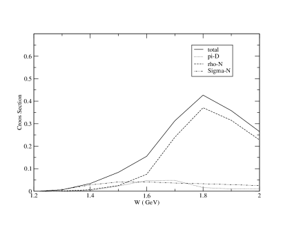
Figure 3: Calculated $\pi N\rightarrow\pi\pi N$ cross sections in $S_{11}$ channel. The partial cross sections through intermediate $\pi\Delta$ (pi-D), $\rho N$ (rho-N) and $\sigma N$ (Sigma-N) are also shown to compare with the coherent sum of these channels (Total),

To obtain reliable information for the second $S_{11}$ resonance at about 1.6 GeV, we are in the process of including $\rho N$ and $\sigma N$ channels. The importance of these two channels can be examined in a unitary calculation of $\pi N\rightarrow\pi\pi N$ cross sections. This is achieved by using the Spline-function expansion method which was developed in our previous investigations of $\pi NN$ problem. Our results of the partial cross sections of $\pi N\rightarrow\pi\pi N$ in $S_{11}$ channel are shown in Fig.3. Clearly, $\rho N$ channel must be included for a dynamical interpretation of the second $N^{*}$ and to establish whether there exists third or even fourth $N^{*}$ in this channel. Our approach is clearly different from the investigation of Chen et al.[16] who include only $\pi N$ and $\eta N$ channels and the fits to the data are achieved by including up to four $N^{*}$.

4 Summary

We have given a unified derivation of most of the models for electromagnetic meson production reactions in the nucleon resonance region. An extension of the coupled-channel approach to include $\pi\pi N$ channel is briefly described and some preliminary results for the $N^{*}(1535)$ excitation have been presented. Our complete calculations will be published elsewhere[22].

References

- [1] T. Sato and T.-S. H. Lee, Phys. Rev. C 54, 2660 (1996); Phys. Rev. C63, 055201 (2001).
- [2] Kamalov and S.N. Yang, Phys. Rev. Lett. 83, 4494 (1999); S.S. Kamalov, S. N. Yang, D. Drechsel, O. Hanstein, and L. Tiator, Phys, Rev, C64, 032201(R) (2001),
- [3] D. Drechsel, O. Hanstein, S.S. Kamalov, and L. Tiator, Nucl. Phys. A645, 145 (1999)
- [4] I. G. Aznauryan, Phys. Rev. C68, 065204 (2003)
- [5] R.L. Walker, Phys. Rev. 182, 1729 (1969)
- [6] R.A. Arndt, I.I. Strakovsky, R.L. Workman, Int. J. Mod. Phys. A18, 449 (2003)
- [7] G. Penner and U. Mosel, Phys. Rev. C66, 055211 (2002); C66, 055212 (2002).
- [8] D. M. Manley, Int. J. of Mod. Phys., A18, 441 (2003);
- [9] R.E. Cutkosky, C.P. Forsyth, R.E. Hendrick, and R.L. Kelly, Phys. Rev. D20, 2839 (1979).
- [10] M. Batinic, I. Slaus, and A. Svarc, Phys. Rev. C51, 2310 (1995)
- [11] T.P. Vrana, S.A. Dytman, and T.-S. H. Lee, Phys. Rept. 328, 181 (2000).
- [12] Yoshimoto, T. Sato, M. Arima, and T.-S. H. Lee, Phys. Rev. C61 065203 (2000).
- [13] Y. Oh, A. Titov, and T.-S. H. Lee, Phys. Rev. C63, 025201 (2001).
- [14] Y. Oh and T.-S. H. Lee, Phys. Rev. C66, 045201 (2002).
- [15] W.-T. Chiang, F. Tabakin, T.-S. H. Lee and B. Saghai, Phys. Lett. B517, 101 (2001).
- [16] G.-Y. Chen, S.S. Kamalov, S. N. Yang, D. Drechsel, and L. Tiator, Nucl. Phys. A723, 447 (2003).
- [17] O. Krehl, C. Hanhart, S. Krewald, and J. Speth, Phys. Rev. C62, 025270 (2000)
- [18] M. G. Fuda and H. Alharbi, Phys. Rev. C68, 064002 (2003).
- [19] F. Gross and Y.Surya, Phys. Rev. C47, 703 (1993); Y.Surya and F. Gross, Phys. Rev. C 53, 2422 (1996).
- [20] N. Kaiser, T. Waas, and W. Weise, Nucl. Phys. A612, 297 (1997).
- [21] E. Oset and A. Ramos, Nucl. Phys. A635, 99 (1998).
- [22] T.-S. H. Lee, A. Matsuyama, and T. Sato, in preparation
- [23] S. Capstick, Phys. Rev.D46, 2864 (1992).