nucl-th/0405077

TUM-T39-04-06

Explicit Delta(1232) Degrees of Freedom in Compton Scattering off the Deuteron

Robert P. Hildebrandt^a,, Harald W. Grießhammer^a,b,,

Thomas R. Hemmert^a,b, and Daniel R. Phillips^c,

^a Institut für Theoretische Physik (T39), Physik-Department,
Technische Universität München, D-85747 Garching, Germany

^b ECT*, Villa Tambosi, I-38050 Villazzano (Trento), Italy

^c Department of Physics and Astronomy, Ohio University, Athens, OH 45701

We examine elastic Compton scattering off the deuteron for photon energies between 50 MeV and 100 MeV in the framework of chiral effective field theories to next-to-leading order. We compare one theoretical scheme with only pions and nucleons as explicit degrees of freedom to another in which the $\Delta(1232)$ resonance is treated as an explicit degree of freedom. Whereas pion degrees of freedom suffice to describe the experimental data measured at about 70 MeV, the explicit $\Delta(1232)$ gives important contributions that help to reproduce the angular dependence at higher energies. The static isoscalar dipole polarizabilities $\alpha_{E}^{s}$ and $\beta_{M}^{s}$ are fitted to the available data, giving results for the neutron polarizabilities $\alpha_{E}^{n}=(14.2\pm 2.0\,(\mathrm{stat})\pm 1.9\,(\mathrm{syst}))\cdot 10^{-4}\;\mathrm{fm}^{3}$, $\beta_{M}^{n}=(1.8\pm 2.2\,(\mathrm{stat})\pm 0.3\,(\mathrm{syst}))\cdot 10^{-4}\;\mathrm{fm}^{3}$. These values are in good agreement with previous experimental analyses. Comparing them to the well-known proton values we conclude that there is currently no evidence for significant differences between the proton and neutron electromagnetic dipole polarizabilities.

Suggested PACS numbers: 13.40.-f, 13.60.Fz, 25.20.-x, 21.45.+v Suggested Keywords: Effective Field Theory, Compton Scattering, Deuteron, Delta Resonance, Nucleon Polarizabilities.

1 Introduction

The structure of protons and neutrons as analyzed with electromagnetic probes has been under experimental and theoretical investigation for a number of decades. In Compton scattering the external electromagnetic field of the photon attempts to deform the nucleon. The electromagnetic polarizabilities provide a measure of the global resistance of the nucleon’s internal degrees of freedom against displacement in an external electric or magnetic field, which makes them an excellent tool to study the sub-nucleonic degrees of freedom. If one defines the polarizabilities via a multipole expansion in Compton scattering, these quantities are energy dependent. The physics connected with this energy dependence is discussed in Refs. [1, 2]. In this work we are mainly concerned with the static values, which we therefore denote as the polarizabilities for simplicity. Experimentally the best-known nucleon polarizabilities are the static electric and magnetic dipole polarizabilities of the proton, $\alpha_{E}^{p}$ and $\beta_{M}^{p}$. The results of the global fit to the wealth of Compton scattering data on the proton given in Ref. [3] are

$$\alpha_{E}^{p} =(12.1\pm 0.3\,(\mathrm{stat})\mp 0.4\,(\mathrm{syst})\pm 0.3\,(\mathrm{model}))\cdot 10^{-4}\;\mathrm{fm}^{3}\,,$$

$$\beta_{M}^{p} =(1.6\pm 0.4\,(\mathrm{stat})\pm 0.4\,(\mathrm{syst})\pm 0.4\,(\mathrm{model}))\cdot 10^{-4}\;\mathrm{fm}^{3}\,.$$ (1)

The values from a Baldin Sum Rule constrained fit of the proton Compton data within the framework that we use in this work, reported in Ref. [2], agree within error bars with (1):

$$\alpha_{E}^{p}=(11.04\pm 1.36)\cdot 10^{-4}\;\mathrm{fm}^{3}\,,\;\;\;\;\beta_{M}^{p}=(2.76\mp 1.36)\cdot 10^{-4}\;\mathrm{fm}^{3}\,.$$ (2)

The errors displayed in Eq. (2) are only statistical. For the fit, the central value of the Baldin Sum Rule $\alpha_{E}^{p}+\beta_{M}^{p}=(13.8\pm 0.4)\cdot 10^{-4}\;\mathrm{fm}^{3}$ [3] has been used.

Due to the lack of stable single-neutron targets for Compton scattering it is much harder to access the neutron polarizabilities experimentally. An experiment on quasi-free Compton scattering from the proton and neutron bound in the deuteron [4] gives results for the neutron polarizabilities which suggest very small isovectorial components when compared to Eqs. (1,2):

$$\alpha_{E}^{n} =(12.5\pm 1.8\,(\mathrm{stat})\,^{+1.1}_{-0.6}\,(\mathrm{syst})\pm 1.1\,(\mathrm{model}))\cdot 10^{-4}\;\mathrm{fm}^{3}$$

$$\beta_{M}^{n} =(2.7\mp 1.8\,(\mathrm{stat})\,^{+0.6}_{-1.1}\,(\mathrm{syst})\mp 1.1\,(\mathrm{model}))\cdot 10^{-4}\;\mathrm{fm}^{3}$$ (3)

A similar observation for $\alpha_{E}^{n}$ has been made in [5], where the scattering of neutrons on lead was measured:

$$\alpha_{E}^{n}=(12.6\pm 2.5)\cdot 10^{-4}\;\mathrm{fm}^{3}$$ (4)

However, the precision of this result has been questioned by the authors of [6]. Their estimate of the correct range for the result from [5] is $7\leq\alpha_{E}^{n}\leq 19$. On the other hand, another experiment [7], using the same technique, gives a completely different result:

$$\alpha_{E}^{n}=(0.6\pm 5.0)\cdot 10^{-4}\;\mathrm{fm}^{3}$$ (5)

On the theory side Chiral Perturbation Theory predicts that the proton and neutron polarizabilities are equal at leading-one-loop order [8], since the pion loops that generate these contributions are isoscalar in nature. The absence of large isovector pieces in $\alpha_{E}$ and $\beta_{M}$ therefore is in accord with this picture.

Another possible way to determine the neutron polarizabilities is elastic low-energy Compton scattering from light nuclei, e.g. from the deuteron. Several experiments have already been performed [9, 10, 11] and further proposals exist – e.g. Compton scattering on the deuteron or $\mathrm{He}^{3}$ at TUNL/HI$\gamma$S [12] and on deuteron targets at MAXlab [13]. From a theorist’s point of view, extracting the neutron polarizabilities from elastic $\gamma d$ scattering requires an accurate description of the nucleon structure and the dynamics of the low-energy degrees of freedom within the deuteron, as one has to correct for the proton polarizabilities and meson-exchange effects. A first attempt to fit the isoscalar polarizabilities $\alpha_{E}^{s}\equiv\frac{1}{2}\,(\alpha_{E}^{p}+\alpha_{E}^{n})$, $\beta_{M}^{s}\equiv\frac{1}{2}\,(\beta_{M}^{p}+\beta_{M}^{n})$ to the elastic deuteron Compton scattering data from [9, 11] has been made in [14]. The extracted neutron polarizabilities $\alpha_{E}^{n}=(9.0\pm 3.0)\cdot 10^{-4}\;\mathrm{fm}^{3}$, $\beta_{M}^{n}=(11.0\pm 3.0)\cdot 10^{-4}\;\mathrm{fm}^{3}$ indicate the possibility of a rather large isovector part. On the other hand comparison of the elastic deuteron Compton calculation of Ref. [15] with the data from [9] is in good agreement with nearly vanishing isovector polarizabilities: $\alpha_{E}^{n}=(12.0\pm 4.0)\cdot 10^{-4}\;\mathrm{fm}^{3}$, $\beta_{M}^{n}=(2.0\pm 4.0)\cdot 10^{-4}\;\mathrm{fm}^{3}$, albeit within rather large error bars.

It is obvious from these partly contradictory results that there is still a lot of work to be done in order to have reliable values for $\alpha_{E}^{n}$ and $\beta_{M}^{n}$. In general, Chiral Effective Field Theory provides a consistent, controlled framework for elastic $\gamma d$ scattering within which nucleon effects can be disentangled from meson-exchange currents, deuteron binding, etc. It therefore gives valuable contributions to the ongoing discussion on the neutron polarizabilities. This work aims for an improved description of elastic deuteron Compton data at $\omega\sim 50$-100 MeV, compared to the calculations presented in [14, 15], which cannot match the data in this regime.

Our work is based on the calculation of Refs. [16, 17], where Compton scattering off the deuteron was examined for photon energies $\omega$ ranging from 50 MeV to 100 MeV. The central values for the isoscalar polarizabilities, derived in the recent analysis [17] of the data from [9, 10, 11] are

$$\alpha_{E}^{s} =(8.9\pm 1.5)^{+4.5}_{-0.9}\cdot 10^{-4}\;\mathrm{fm}^{3}\;,$$

$$\beta_{M}^{s} =(2.2\pm 1.5)^{+1.2}_{-0.9}\cdot 10^{-4}\;\mathrm{fm}^{3}\;.$$ (6)

Comparing with Eq. (1), these results indicate a small isovector magnetic polarizability, but signal the possibility of a rather large $\alpha_{E}^{v}$. However, the range for $\alpha_{E}^{s}$ and $\beta_{M}^{s}$ quoted in [17] is rather large: $\alpha_{E}^{s}=(8.0-13.6)\cdot 10^{-4}\;\mathrm{fm}^{3}$, $\beta_{M}^{s}=(1.3-3.4)\cdot 10^{-4}\;\mathrm{fm}^{3}$. The authors of Ref. [16] followed Weinberg’s proposal to calculate the irreducible kernel for the $\gamma NN\rightarrow\gamma NN$ process in Heavy Baryon Chiral Perturbation Theory (HB$\chi$PT) and then fold this with external deuteron wave functions such as Nijm93 [18], CD-Bonn [19] or AV18 [20]. Proceeding in this fashion means working within an Effective Field Theory in which only nucleons and pions are active degrees of freedom. This “hybrid” approach has proven quite successful in describing $\pi d$ [21], $e^{-}d$ [22], and even $\gamma d$ [16, 17] scattering. In this work we extend the calculation of Ref. [16] to an Effective Field Theory which includes the $\Delta(1232)$ resonance of the nucleon as an additional explicit degree of freedom. The advantage of our approach with respect to the NNLO calculation of Ref. [17] is that we identify the physics hidden in some of the short-distance parameters there. As we shall see, this is particularly important for quantities such as the magnetic polarizability $\beta_{M}$, where the $\Delta(1232)$ plays an important dynamical role. The huge influence of the $\Delta(1232)$ in single-nucleon Compton scattering – especially in the backward direction – is a well-known fact (see e.g. [2]). We note that the importance of the $\Delta$-contributions is due to the strong paramagnetic $M1$ coupling of the photon to the $N\rightarrow\Delta$ transition, visible already far below resonance (cf. [2]). It is therefore interesting to also investigate the role of these degrees of freedom in elastic $\gamma d$ scattering, and this is the main focus of our work.

The idea of an extension of HB$\chi$PT that includes explicit $\Delta$ degrees of freedom has its origin in the early 1990’s [23]. When including the $\Delta(1232)$ explicitly in $\chi$EFT one needs to specify how the $\Delta N$ mass splitting $\Delta_{0}$ is treated in the power counting. Here we use the so-called Small Scale Expansion (SSE) [24]. We note that there also exist alternative approaches for Chiral Effective Field Theories with explicit $\pi$, $N$ and $\Delta$ degrees of freedom, e.g. the $\delta$-expansion [25], which was recently shown to describe $\gamma p$ cross section data well in an energy range from $\omega=0$ MeV to $\omega=300$ MeV.

In Sect. 3 we discuss our predictions for the deuteron Compton cross sections for three different energies between 50 MeV and 100 MeV, comparing to experimental data and to the $\mathcal{O}(q^{3})$ HB$\chi$PT calculation [16]. Before that, we give a brief survey of the theoretical formalism in Sect. 2. There we show that combining Weinberg’s counting ideas with the SSE power counting scheme leads to no additional diagrams in the two-body part of the kernel with respect to [16]. In Sect. 4 we present our results for the isoscalar polarizabilities, derived from a fit to elastic deuteron Compton scattering data, which turn out to be in good agreement with the theoretical expectation that the isovector components are small. We conclude in Sect. 5 and give a brief outlook on future projects, one of which aims to cure the shortcomings of our calculation in the extreme low-energy regime $\omega\ll 50$ MeV (cf. Sect. 2).

2 Compton Scattering off the Deuteron in Effective Field Theory

We are calculating Compton scattering off the deuteron in the framework of the Small Scale Expansion [24], an Effective Field Theory with nucleons, pions and the $\Delta(1232)$ resonance as explicit degrees of freedom. In this extension of $\chi$PT, the expansion parameter is called $\epsilon$, denoting either a small momentum, the pion mass or the mass difference $\Delta_{0}$ between the real part of the $\Delta$ mass and the nucleon mass. The relevant pieces of the $N\pi$ and $\Delta\pi$ Lagrangeans have been discussed in the literature many times, and we refer the interested reader to [26] for the $N\pi$ Lagrangean and for a general review of HB$\chi$PT, and to [27] and [2] for the relevant pieces of the $\Delta\pi$ Lagrangean.

The power-counting scheme that we use for Compton scattering off light nuclei is motivated by Weinberg’s idea to count powers only in the interaction kernel. We base our calculation on the hybrid approach, which is a well-established tool by now. While the kernel is power counted according to the rules of the Effective Field Theory, the deuteron wave functions we use are obtained from state-of-the-art $NN$ potentials: Nijm93 [18], the CD-Bonn potential [19], the AV18 potential [20] and the NNLO chiral potential [28], where this last potential also follows Weinberg’s suggestion, and is derived by applying HB$\chi$PT power counting to the $NN$ potential $V$.

It is convenient to write the Green’s function for Compton scattering from the two-nucleon system as

$$G_{\gamma\gamma}=G\,K_{\gamma\gamma}\,G+G\,K_{\gamma}\,G\,K_{\gamma}\,G\,,$$ (7)

with $K_{\gamma\gamma}$ the two-nucleon-irreducible part of the interaction kernel, which contains both one-body and two-body mechanisms, and $K_{\gamma}\,G\,K_{\gamma}$ the so-called nuclear-resonance contribution to the kernel. $G$ is the two-particle Green’s function, constructed from the two-nucleon-irreducible interaction $V$ and the free two-nucleon Green’s function. We apply the same power counting rules to both $K_{\gamma\gamma}$ and $K_{\gamma}GK_{\gamma}$, calculating all contributions up to a specific order in $\epsilon$, namely $\epsilon^{3}$.

To do this we first note that a diagram contributing at a certain order in $q$ in HB$\chi$PT contributes at the same order $\epsilon$ in SSE. However, there are some kinematics in which HB$\chi$PT counting should not be employed for the $\gamma NN\rightarrow\gamma NN$ kernel. In HB$\chi$PT the leading order propagator of a nucleon with the energy $\omega$ of the external probe flowing through it is $\frac{i}{\omega}$. Corrections from the kinetic energy of the nucleon are treated perturbatively. In the deuteron, such a perturbative treatment is not applicable for low photon energies, due to the relative momentum $\vec{p}$ of the two nucleons. Therefore, in the low-energy regime one has to use the full non-relativistic nucleon propagator $\frac{i}{\omega-p^{2}/2M}$. Nonetheless, the approximation $\frac{i}{\omega}$ is useful for $\omega\gg B$, with $B\approx 2.225$ MeV the binding energy of the deuteron, as $p^{2}/M\sim B$ with a typical nucleon momentum $p$ inside the deuteron. These considerations demonstrate that for $\omega\gg B$ the nucleon propagator may be counted as $\mathcal{O}(\epsilon^{-1})$ like in standard HB$\chi$PT, whereas in the ‘nuclear’ regime $\omega\sim\mathcal{O}(m_{\pi}^{2}/M)$ it has to be counted as $\mathcal{O}(\epsilon^{-2})$, as $p\sim\epsilon$. Therefore, one has to strictly differentiate between two energy regimes: the nuclear regime $\omega\sim\mathcal{O}(m_{\pi}^{2}/M)$ and the regime $\omega\sim\mathcal{O}(m_{\pi})$. Here we work in the latter one, as we are mainly concerned with photon energies $\omega\geq 50$ MeV, which is the energy region where one starts to be sensitive to the nucleon polarizabilities.

We note further that only in the regime $\omega\sim\mathcal{O}(m_{\pi})$ can one treat the contributions from $K_{\gamma}GK_{\gamma}$ using a perturbative chiral expansion. Since we do treat this piece using HB$\chi$PT counting it is therefore no surprise that the Compton low-energy theorems are violated. For example, the Thomson limit for Compton scattering from a nucleus of charge $Z\,e$ and mass $A\,M$,

$$A_{\mathrm{Thomson}}=A(\omega=0)=-\frac{Z^{2}\,e^{2}}{A\,M}\,\vec{\epsilon}\cdot\vec{\epsilon}\,^{\prime}\,,$$ (8)

a direct consequence of gauge invariance [29], cannot be recovered without the full resonance term. Therefore, we strictly constrain ourselves to photon energies $\omega\sim\mathcal{O}(m_{\pi})$, where a perturbative expansion of the kernel in the standard HB$\chi$PT counting scheme, i.e. counting the nucleon propagator as $\mathcal{O}(\epsilon^{-1})$, is possible. The lower limit of this power counting turns out to be $\omega\approx 50$ MeV, so we have to caution the reader that the calculation is not supposed to work in the region $\omega\ll 50$ MeV (an extension to lower energies is in progress [30]). A more detailed discussion of the power counting applied to the meson exchange part of our calculation can be found in Refs. [16, 17]. For an Effective Field Theory approach to deuteron Compton scattering where pions are integrated out, see Ref. [31]. These calculations describe the very-low-energy region well and also reach the exact Thomson limit.

The $T$-matrix for Compton scattering off the deuteron is derived as the matrix element of the interaction kernel, evaluated between an initial and final state deuteron wave function, as explained in great detail in [16],

$$T=\left<\Psi_{f}|K_{\gamma\gamma}+K_{\gamma}\,G\,K_{\gamma}|\Psi_{i}\right>\,.$$ (9)

Stated differently, one obtains $T$ by extracting the piece of $G_{\gamma\gamma}$ corresponding to the deuteron pole at $E=-B$ in both the initial and final state.

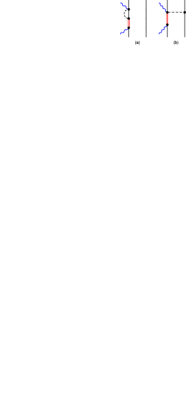
As we are calculating $\gamma d$ scattering in the Small Scale Expansion, we also have to fix our counting rules for diagrams including $\Delta(1232)$ propagators. For the one-body contributions this is straightforward, as we apply the SSE counting scheme, cf. Refs. [2, 32]. As far as the two-body physics is concerned, we combine the SSE counting rules, e.g. counting the $\Delta$-propagator as $\epsilon^{-1}$, with Weinberg’s prescription of counting only within the interaction kernel. To $\mathcal{O}(\epsilon^{3})$, the order up to which we are working, this leads to identical meson exchange diagrams as in the $\mathcal{O}(q^{3})$ HB$\chi$PT calculation. All additional diagrams are at least one order higher, an example is given in Fig. 1(b) (an example of an $\mathcal{O}(\epsilon^{4})$ one-body diagram is sketched in Fig. 1(a)). A modified counting scheme in the two-body sector has been suggested in [21], as certain pion-exchange diagrams may be enhanced when the photon energy comes close enough to the pion mass that the pions in the two-body diagrams are almost on mass shell. We do not consider such a modification necessary for our calculation, as we restrict ourselves to photon energies $\omega\leq 100$ MeV.

Figure 1: Two examples of $\mathcal{O}(\epsilon^{4})$ contributions to Compton scattering on the deuteron including explicit $\Delta(1232)$ degrees of freedom for one- and two-body contributions.

Therefore, the diagrams contributing to deuteron Compton scattering up to $\mathcal{O}(\epsilon^{3})$ are:

• One-body contributions without explicit $\Delta(1232)$ degrees of freedom. These are the single-nucleon seagull with the two-photon vertex from $\mathcal{L}_{N\pi}^{(2)}$ (Fig. 2(a)), which is the only $\mathcal{O}(\epsilon^{2})$ contribution, the nucleon-pole terms (Fig. 2(b)), the pion pole (Fig. 2(c)) and the contributions from the leading chiral dynamics of the pion cloud around the nucleon (Figs. 2(d)-(g)). Up to third order, the only difference in these diagrams, compared to Compton scattering off the single nucleon, is that the pole diagrams (Fig. 2(b)), which are conveniently calculated in the $\gamma N$ center of mass frame, have to be boosted to the $\gamma NN$ center of mass system, as the calculation is performed in the $\gamma d$ cm frame. The resulting formulae from the boost are given in [16].

  

  

  

  

  

  

  

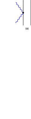
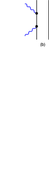
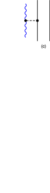
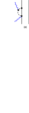
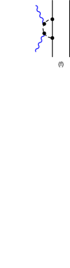
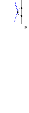
  Figure 2: One-body interactions without a $\Delta(1232)$ propagator contributing to Compton scattering on the deuteron up to $\mathcal{O}(\epsilon^{3})$ in SSE. Permutations and crossed graphs are not shown.

• One-body diagrams with explicit $\Delta$ degrees of freedom, as shown in Fig. 3: The $\Delta$-pole diagrams (Fig. 3(a)) and the contributions from the pion cloud around the $\Delta(1232)$ (Figs. 3(b)-(e)).

• Two isoscalar short-distance one-body operators (Fig. 3(f)), which give energy-inde-pendent contributions to the dipole polarizabilities $\alpha_{E}^{s}$ and $\beta_{M}^{s}$. They are formally of $\mathcal{O}(\epsilon^{4})$ but turn out to give an anomalously large contribution to the single-nucleon Compton amplitude. Therefore, they have to be promoted to next-to-leading order as discussed in detail in [2], which we also refer to for the Lagrangean. We note that except for the two contact operators (Fig. 3(f)), the $\delta$-expansion (cf. Sect. 1) up to NNLO is equivalent to $\mathcal{O}(\epsilon^{3})$ SSE in the energy range $\omega\sim m_{\pi}$ considered.

  

  

  

  

  

  

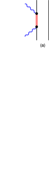
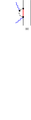
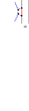
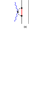
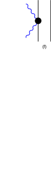
  Figure 3: One-body interactions which contribute to deuteron Compton scattering at $\mathcal{O}(\epsilon^{3})$ in SSE in addition compared to third-order HB$\chi$PT. Permutations and crossed graphs are not shown.

• Two-body contributions with one pion exchanged between the two nucleons (Fig. 4). In total there are nine two-body diagrams at $\mathcal{O}(\epsilon^{3})$. As discussed before, the meson exchange diagrams are identical in third-order HB$\chi$PT and SSE.

  
  

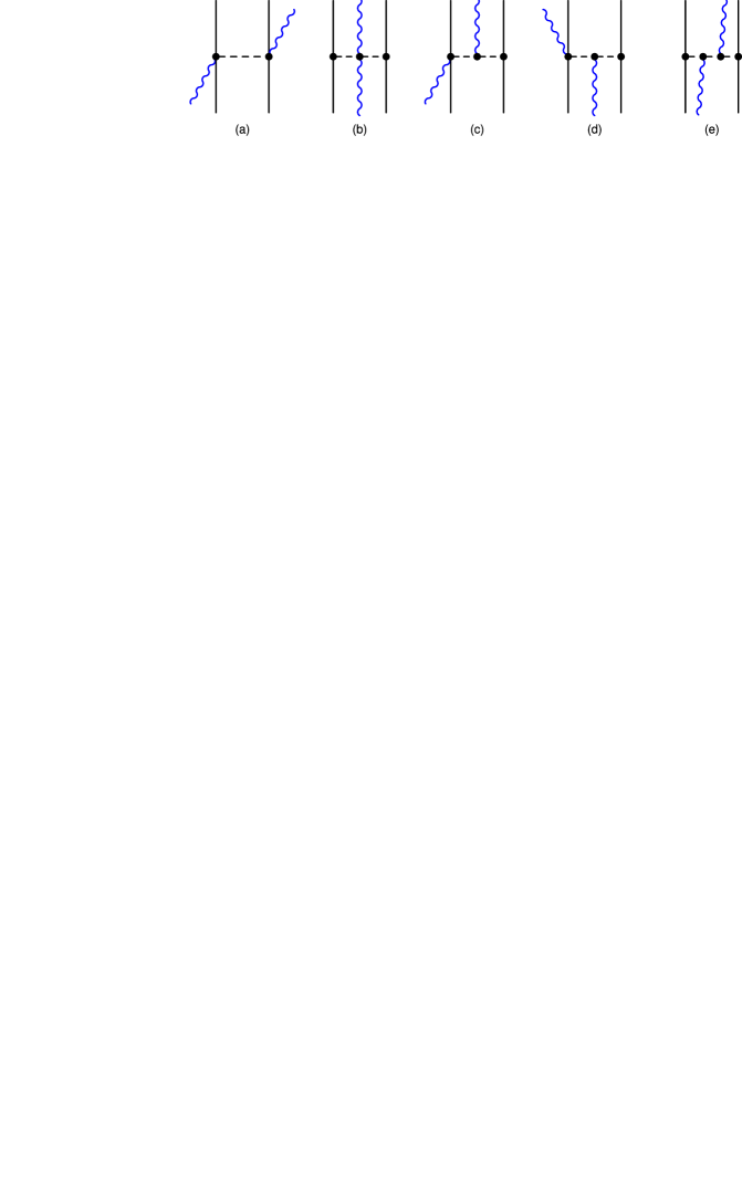
  Figure 4: Two-body interactions contributing to the kernel for Compton scattering on the deuteron at $\mathcal{O}(\epsilon^{3})$ in SSE. Diagrams which differ only by nucleon interchange are not shown.

All these diagrams (Figs. 2–4) make up our interaction kernel. The SSE single-nucleon amplitudes can be found in [2], while the two-body contributions are given explicitly in [16]. Note that we have simplified the expressions given in [2] with respect to the exact position of the pion threshold as we are only analysing Compton scattering for photon energies $\leq 100$ MeV. An estimate of the (small) size of this simplification is given in Sect. 3.2.

In the next section we compare our $\mathcal{O}(\epsilon^{3})$ SSE results for the deuteron Compton cross sections to the $\mathcal{O}(q^{3})$ HB$\chi$PT calculation performed in [16] and to the available experimental data. Special interest is put on the energy and wave-function dependence of the cross section.

3 Predictions for Deuteron Compton Cross Sections

Figure 5: Comparison of the $\mathcal{O}(q^{3})$ HB$\chi$PT (dashed) and the $\mathcal{O}(\epsilon^{3})$ SSE (solid) prediction at $\omega_{\mathrm{lab}}=49\;\mathrm{MeV}$, $\omega_{\mathrm{lab}}=69\;\mathrm{MeV}$ and $\omega_{\mathrm{lab}}=94.2\;\mathrm{MeV}$ using the chiral NNLO wave function [28]. The data are from Illinois [9] (circle), Lund [10] (star) and SAL [11] (diamond). The dotted line is the $\mathcal{O}(q^{2})$ result.

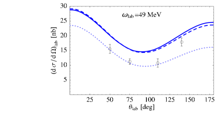
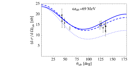
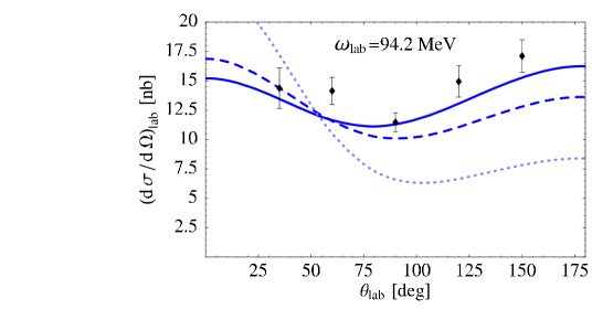
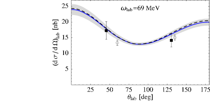
In Fig. 5 we compare the $\mathcal{O}(\epsilon^{3})$ SSE predictions to the $\mathcal{O}(q^{3})$ HB$\chi$PT calculation of Ref. [16], using the wave function derived from the NNLO chiral potential with spectral function regularization [28]. We also show the $\mathcal{O}(q^{2})$ result, which consists only of the single-nucleon seagull (Fig. 2(a)). The experiments shown have been performed at a lab-energy of 49 MeV [9], $\sim$67 MeV [10], 69 MeV [9] and $\sim$94.2 MeV [11]. (The last experiment used photons in an energy range from $84.2-104.5$ MeV; the deviation from the central value has been corrected for [11].)

The values we use for physical constants can be found in Table 1. For the coupling constants connected with the two short-distance $\gamma N$-operators (cf. Sect. 2) and the $\gamma N\Delta$ coupling $b_{1}$ we use the results of the Baldin Sum Rule constrained fit to the spin-averaged proton Compton scattering data from [2]. Fitting the short-distance operators is equivalent to fitting the static polarizabilities $\alpha_{E}^{p}$, $\beta_{M}^{p}$. We use the central values of the fit, which are $\alpha_{E}^{p}=11.04\cdot 10^{-4}\;\mathrm{fm}^{3}$, $\beta_{M}^{p}=2.76\cdot 10^{-4}\;\mathrm{fm}^{3}$ [2], cf. Sect. 1. The $\mathcal{O}(\epsilon^{3})$ SSE calculation then predicts $\alpha_{E}^{n}\equiv\alpha_{E}^{p}$, $\beta_{M}^{n}\equiv\beta_{M}^{p}$ as the isovector contributions only come in at $\mathcal{O}(\epsilon^{4})$. Therefore, there are no free parameters in our deuteron Compton calculation.

Parameter	Value	Comment
$m_{\pi}$	$139.6$ MeV	charged pion mass
$M$	$938.9$ MeV	isoscalar nucleon mass
$f_{\pi}$	$92.4$ MeV	pion decay constant
$g_{A}$	$1.267$	axial coupling constant
$\alpha$	$1/137$	QED fine structure constant
$\kappa_{v}$	$3.708$	isovector anomalous magnetic moment
$\kappa_{s}$	$-0.118$	isoscalar anomalous magnetic moment
$M_{d}$	$1875.58$ MeV	deuteron mass
$B$	$2.2246$ MeV	deuteron binding energy
$\Delta_{0}$	$271.1$ MeV	$N\Delta$ mass splitting
$g_{\pi N\Delta}$	$1.125$	$\pi N\Delta$ coupling constant
$b_{1}$	$4.67$	$\gamma N\Delta$ coupling constant
$g_{117}$	$18.82$	short-distance coupling constant
$g_{118}$	$-6.05$	short-distance coupling constant

Table 1: $\chi$EFT parameters determined independently of deuteron Compton scattering. Magnetic moments are given in nuclear magnetons.

From the 49 and 69 MeV curves shown in Fig. 5 it is obvious that explicit $\Delta$ degrees of freedom may well be neglected for these low energies. The two calculations – HB$\chi$PT and SSE – yield results which differ only within the uncertainties one expects from higher order contributions. This is an important check, as it demonstrates the correct decoupling of the resonance, which provides the same low-energy limit in both theories.

Another interesting observation can be made: The counting scheme described in Sect. 2 seems to break down for energies somewhere near 50 MeV, as both theoretical descriptions miss the 49 MeV data points, whereas the 69 MeV data (we neglect the minor corrections due to the data of [10] being measured around 67 MeV) are well described within both theories. The 49 MeV data are best described by the $\mathcal{O}(q^{2})$ calculation but we believe this is a coincidence, as the low-energy theorems are violated at this order too. However, for higher energies – i.e. for describing the 94.2 MeV data correctly – the inclusion of the explicit $\Delta$ field seems to be advantageous in a third-order calculation. Here, $\mathcal{O}(q^{3})$ $\chi$PT misses the data in the backward direction. It also fails to reproduce the shape of the data points, which shows a slight tendency towards higher cross sections in the backward than in the forward direction. This shape is very well reproduced in SSE, demonstrating once again the importance of the $\Delta$ resonance in Compton backscattering, due to the strong $M1\rightarrow M1$ transition. We note that this feature can be clearly seen in the dynamical magnetic dipole polarizability $\beta_{M1}(\omega)$, even for photon energies below the pion-production threshold (cf. [2] and Sect. 4.3). Calculations like the ones presented in Refs. [14, 15], which include the dynamics of the polarizabilities only via the leading [14, 15] and subleading terms [14] of a Taylor expansion, may therefore fail to describe the data around 95 MeV.

3.1 Energy Dependence of the $\gamma d$ Cross Sections

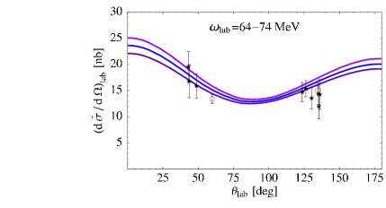
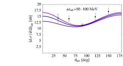
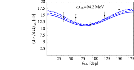
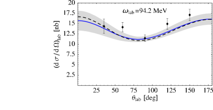
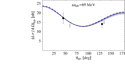
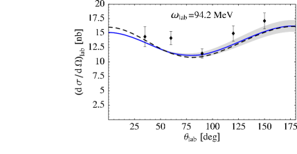
In order to decrease the statistical uncertainties, the experiment [11] had to accept scattering events in an energy range of around 20 MeV. Therefore we think it worthwhile to examine the sensitivity of our results to the photon energy. In fact, our calculations suggest that the forward-angle cross section, in particular, has a sizeable energy dependence, which is, however, nearly linear. In Fig. 6 we show our results for three different photon energies around 69 MeV and 94.2 MeV, respectively, separated only by 10 MeV. This emphasizes the importance of having a well-defined photon energy at which to examine the effects of $\alpha_{E}$ and $\beta_{M}$.

Figure 6: $\mathcal{O}(\epsilon^{3})$ SSE results for 64 MeV, 69 MeV, 74 MeV and, respectively, 90 MeV, 94.2 MeV, 100 MeV (from the upper to the lower curve in each panel), using the $\chi$PT wave function [28].

3.2 Correction due to the Pion-Production Threshold

Figure 7: Estimate of the effect of a threshold correction (dotdashed) on the $\mathcal{O}(\epsilon^{3})$ SSE results (solid), using the chiral NNLO wave function [28].

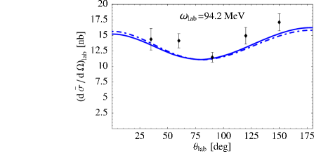
In low-order HB$\chi$PT/SSE calculations the $\gamma d\rightarrow\pi NN$ threshold is not at the correct position as dictated by relativistic kinematics. For a similar problem, regarding the correct position of the pion-production threshold in the single-nucleon sector, see e.g. [2]. So far we refrain from an analogous correction for $\gamma d$ scattering. However, in Fig. 7 we investigate what deviations one would expect from our present results, as indicated by an estimate, where we use the single-nucleon SSE amplitudes [2] with the exact expression for $\sqrt{s}-M$. Obviously, even at the highest photon energies considered here, 94.2 MeV, the corrections are negligible, given the sizeable error bars of the experimental data and the theoretical uncertainties of a leading-one-loop order calculation.

3.3 Wave-Function Dependence of the $\gamma d$ Cross Sections

Figure 8: $\mathcal{O}(\epsilon^{3})$ SSE results for 69 and 94.2 MeV, using four different wave functions: NNLO $\chi$PT [28] (solid), Nijm93 [18] (dotted), CD-Bonn [19] (dashed), AV18 [20] (dotdashed).

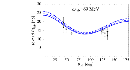
Another interesting issue is the wave-function dependence of our results. Fig. 8 investigates the sensitivity to the wave function chosen, showing sizeable deviations between the NNLO $\chi$PT wave function [28] on one hand and the wave functions derived from the Nijm93 potential [18] and the AV18 potential [20] on the other. The last two yield results which are nearly indistinguishable but are considerably higher than those found with the wave function of [28]. With the CD-Bonn wave function [19] we obtain results in between NNLO $\chi$PT and Nijm93/AV18. This pattern is identical for both energies under investigation, 69 MeV and 94.2 MeV. Given that our calculation is based on a low-energy Effective Field Theory of QCD, the dependence on the wave function is somewhat worrisome and will be discussed further in [30]. According to Weinberg counting it is an $\mathcal{O}(q^{5})$ effect, so a deviation of the order of 10% is more than one would expect. We interpret this feature as an unwanted sensitivity to short-distance physics, because the long-range part of all wave functions, described by one- and two-pion exchange, is identical. However, one must caution that the NNLO $\chi$PT potential reproduces the Nijmegen partial-wave analysis with less precision than the CD-Bonn, AV18 or Nijm93 potentials.

In this section we presented our predictions for $\gamma d$ differential cross sections. These are parameter-free as we fixed the nucleon polarizabilities via proton Compton data. The good agreement of the SSE results with experiment at 69 MeV and 94.2 MeV leaves little room for large isovector polarizabilities, since these predictions used the same values for the proton and neutron polarizabilities. It further encourages us to determine the isoscalar dipole polarizabilities $\alpha_{E}^{s}$ and $\beta_{M}^{s}$ directly from the deuteron Compton cross sections. The results are displayed in the next section, together with the results one obtains from analogous fits using the $\mathcal{O}(q^{3})$ HB$\chi$PT amplitudes.

4 Determining $\alpha_{E}^{s}$ and $\beta_{M}^{s}$ from $\gamma d$ Scattering

An accurate and systematically-improvable description of Compton scattering on deuterium offers the possibility to extract the isoscalar polarizabilities directly from deuteron Compton scattering experiments in a systematic way. The resulting numbers can then be combined with the known numbers for the proton to draw conclusions about isovector pieces $\alpha_{E}^{v}$ and $\beta_{M}^{v}$, or, equivalently, the elusive neutron polarizabilities. As our SSE calculation provides a reasonable description of the 69 MeV and the 94.2 MeV data (see Sect. 3), we present in the following our results from a fit of the isoscalar polarizabilities to these two data sets. This corresponds to fitting the coupling strengths of the two short-distance isoscalar $\gamma N$-operators (Fig. 3(f)), which we now fit to $\gamma d$ data rather than to $\gamma p$ data. In this way we can check our assumption that the short-distance operators are isoscalar at leading order. If the value extracted from $\gamma d$ data is approximately that from $\gamma p$ data, that argues in favour of short-distance mechanisms which are predominantly isoscalar.

Our SSE results are compared to the fit results that we get for $\alpha_{E}^{s}$ and $\beta_{M}^{s}$ when we use modified $\mathcal{O}(q^{3})$ HB$\chi$PT amplitudes. This modification consists of including in our calculation isoscalar short-distance $\gamma N$ operators which change both the electric and magnetic polarizability from their $\mathcal{O}(q^{3})$ values. In other words, we write

$$\alpha_{E}^{s} =\frac{5\,\alpha\,g_{A}^{2}}{96\,f_{\pi}^{2}\,m_{\pi}\,\pi}+\delta_{\alpha}\,,$$

$$\beta_{M}^{s} =\frac{\alpha\,g_{A}^{2}}{192\,f_{\pi}^{2}\,m_{\pi}\,\pi}+\delta_{\beta}\,.$$ (10)

The energy dependence of the polarizabilities is still given solely by the leading-order pion cloud. Eq. (10) promotes the short-distance contribution to $\alpha$ and $\beta$ from $\mathcal{O}(q^{4})$ to $\mathcal{O}(q^{3})$. There are indications that this change in the power counting is necessary if high-energy modes in the pion-loop graphs that generate $\alpha$ and $\beta$ are to be properly accounted for [33]. In order to avoid confusion we denote the fits done with this procedure as HB$\chi$PT $\mathcal{O}(\bar{q}^{3})$.

Fits similar to our $\mathcal{O}(\epsilon^{3})$ and $\mathcal{O}(\bar{q}^{3})$ ones have already been performed in [17], calculating in HB$\chi$PT up to $\mathcal{O}(q^{4})$. The authors of [17] used all available data sets but had to exclude the two 94.2 MeV data points measured in the backward direction. As [16, 17] and the $\mathcal{O}(\epsilon^{3})$ SSE calculation obviously have problems to describe the normalization of the data at energies below 60 MeV we decided to only include the data around 69 MeV [9, 10] and 94.2 MeV [11] in the fit. We do not make any cuts on the angles and, in contradistinction to [17], we do not allow the normalizations in the various experiments to float in the fit within their quoted systematic errors.

We performed the fits using the NNLO chiral wave function. We fitted the 16 data points using 2 free parameters ($\alpha_{E}^{s}$ and $\beta_{M}^{s}$), leaving us with 14 degrees of freedom. The resulting values for $\alpha_{E}^{s}$ and $\beta_{M}^{s}$ (see Table 2) are

$$\alpha_{E}^{s}=(12.1\pm 1.3)\cdot 10^{-4}\;\mathrm{fm}^{3},\;\;\beta_{M}^{s}=(1.8\pm 1.6)\cdot 10^{-4}\;\mathrm{fm}^{3}$$ (11)

with a $\chi^{2}/d.o.f.$ of 1.78. The corresponding plots are displayed in Fig. 9, together with the results of our $\mathcal{O}(\bar{q}^{3})$ fits. Using the experimental values from Eq. (1) [3] as input or, equivalently, the values given in Eq. (2), which are obtained from proton Compton scattering data within the same framework as we are using here, one can derive the neutron polarizabilities from the isoscalar ones:

$$\alpha_{E}^{n}=(12.1\pm 1.3)\cdot 10^{-4}\;\mathrm{fm}^{3},\;\;\beta_{M}^{n}=(2.0\pm 1.6)\cdot 10^{-4}\;\mathrm{fm}^{3}$$ (12)

From these results we deduce that the isovector polarizabilities are rather small (see Table 2), in good agreement with $\chi$PT expectations, which predict the isovector part to be of higher than third order. Therefore we find no contradiction between the results from quasi-free [4] and elastic deuteron Compton scattering.

Our results for $\alpha_{E}^{s}$ and $\beta_{M}^{s}$ in SSE (cf. Eq.(11)) are well consistent (within error bars) with the isoscalar Baldin Sum Rule

$$\alpha_{E}^{s}+\beta_{M}^{s}\bigg{|}_{\mathrm{world}\;\,\mathrm{av.}}=(14.5\pm 0.6)\cdot 10^{-4}\;\mathrm{fm}^{3},$$ (13)

which has been a serious problem in former extractions [14, 17]. The numerical value for the sum rule is derived from

$$\alpha_{E}^{p}+\beta_{M}^{p} =(13.8\pm 0.4)\cdot 10^{-4}\;\mathrm{fm}^{3}\;\;\;\;\;\cite[cite]{[\@@bibref{}{Olmos}{}{}]},$$

$$\alpha_{E}^{n}+\beta_{M}^{n} =(15.2\pm 0.5)\cdot 10^{-4}\;\mathrm{fm}^{3}\;\;\;\;\;\cite[cite]{[\@@bibref{}{Kossert}{}{}]}.$$ (14)

Due to the consistency of our fit results with the sum rule value from Eq. (13) one can in a second step use this number – we use the central value – as an additional fit constraint and thus reduce the number of free parameters to one. The resulting one-parameter fits in SSE of Table 2,

$$\alpha_{E}^{s}=(12.3\pm 0.7)\cdot 10^{-4}\;\mathrm{fm}^{3},\;\;\beta_{M}^{s}=(2.2\mp 0.7)\cdot 10^{-4}\;\mathrm{fm}^{3},$$ (15)

are in good agreement with the isoscalar average of the numbers from Eqs. (1) and (3) – or, alternatively, Eqs. (1) and (4).

Comparing our fit results to the isoscalar $\mathcal{O}(q^{4})$ HB$\chi$PT estimate [34], $\alpha_{E}^{s}=(11.95\pm 2.5)\cdot 10^{-4}\;\mathrm{fm}^{3}$, $\beta_{M}^{s}=(5.65\pm 5.1)\cdot 10^{-4}\;\mathrm{fm}^{3}$, we see only minor deviations from their value for $\alpha_{E}^{s}$. However, our values for $\beta_{M}^{s}$ are significantly smaller, but no meaningful conclusion can be drawn due to the large error bars in the $\mathcal{O}(q^{4})$ estimate. The reason for the huge error bars in the $\mathcal{O}(q^{4})$ HB$\chi$PT numbers of Ref. [34] is their sensitivity to short-distance contributions which were estimated using the resonance-saturation hypothesis.

4.1 Wave-Function Dependence of the Fits

To have an estimate on the systematic error due to the wave-function dependence, we show our results when we use the two extreme wave functions (cf. Fig. 8) for the fit: the NNLO chiral wave function [28] and the wave function from the Nijm93 potential [18]. Furthermore, we are fitting in two different ways: First the number of degrees of freedom is the number of data points (16) minus the number of free parameters (2). In a second step we use the isoscalar Baldin Sum Rule, Eq. (13), to reduce the number of degrees of freedom to 1, as described before.

Fitting the $\gamma d$ cross sections with the $\mathcal{O}(\epsilon^{3})$ and $\mathcal{O}(\bar{q}^{3})$ kernel, respectively, using the Nijm93 wave function yields larger results for $\alpha_{E}$ and smaller ones for $\beta_{M}$, but still the values of Table 2 are in reasonable agreement with the values given in Eq. (3) [4]. Comparing the differing results that we get for $\alpha_{E}^{s}$ with the Nijm93 and the NNLO $\chi$PT wave function, we estimate our systematic error to be of the order of 15 %.

Amplitudes	Quantity	2-par. fit	1-par. fit	2-par. fit	1-par. fit
		NNLO $\chi$PT	NNLO $\chi$PT	Nijm93	Nijm93
$\mathcal{O}(\epsilon^{3})$ SSE	$\chi^{2}/d.o.f.$	1.78	1.67	2.45	2.35
	$\alpha_{E}^{s}\;\,[10^{-4}\,\mathrm{fm}^{3}]$	$12.1\pm 1.3$	$12.3\pm 0.7$	$14.3\pm 1.3$	$13.8\pm 0.7$
	$\beta_{M}^{s}\;\,[10^{-4}\,\mathrm{fm}^{3}]$	$1.8\pm 1.6$	$2.2\mp 0.7$	$1.5\pm 1.6$	$0.7\mp 0.7$
	$\alpha_{E}^{s}+\beta_{M}^{s}\;\,[10^{-4}\,\mathrm{fm}^{3}]$	$13.9\pm 2.1$	$14.5\,(\mathrm{fit})$	$15.8\pm 2.1$	$14.5\,(\mathrm{fit})$
	$\alpha_{E}^{n}\;\,[10^{-4}\,\mathrm{fm}^{3}]$	$12.1\pm 1.3$	$12.5\pm 0.8$	$16.5\pm 1.3$	$15.5\pm 0.8$
	$\beta_{M}^{n}\;\,[10^{-4}\,\mathrm{fm}^{3}]$	$2.0\pm 1.6$	$2.8\pm 0.8$	$1.4\pm 1.6$	$-0.2\pm 0.8$
$\mathcal{O}(\bar{q}^{3})$ HB$\chi$PT	$\chi^{2}/d.o.f.$	2.14	2.01	2.87	2.75
	$\alpha_{E}^{s}\;\,[10^{-4}\,\mathrm{fm}^{3}]$	$11.0\pm 1.3$	$11.3\pm 0.7$	$13.2\pm 1.2$	$12.7\pm 0.7$
	$\beta_{M}^{s}\;\,[10^{-4}\,\mathrm{fm}^{3}]$	$2.8\pm 1.6$	$3.2\mp 0.7$	$2.5\pm 1.5$	$1.8\mp 0.7$
	$\alpha_{E}^{s}+\beta_{M}^{s}\;\,[10^{-4}\,\mathrm{fm}^{3}]$	$13.8\pm 2.1$	$14.5\,(\mathrm{fit})$	$15.7\pm 1.9$	$14.5\,(\mathrm{fit})$
	$\alpha_{E}^{n}\;\,[10^{-4}\,\mathrm{fm}^{3}]$	$9.9\pm 1.3$	$10.5\pm 0.8$	$14.3\pm 1.2$	$13.3\pm 0.8$
	$\beta_{M}^{n}\;\,[10^{-4}\,\mathrm{fm}^{3}]$	$4.0\pm 1.6$	$4.8\pm 0.8$	$3.4\pm 1.5$	$2.0\pm 0.8$

Table 2: Values for the isoscalar and neutron polarizabilities from a fit to the full 69 MeV and 94.2 MeV data sets [9, 10, 11], using the $\mathcal{O}(\epsilon^{3})$ SSE amplitudes and the $\mathcal{O}(\bar{q}^{3})$ HB$\chi$PT amplitudes, respectively. The neutron results are derived using the proton values from [3] (Eq. (1)) as input. All error bars displayed are only statistical.

One of the reasons for the differing results between our approach and the calculations presented in [14, 15] is the energy dependence of the polarizabilities. In our calculation, it is completely given by the Compton multipoles, whereas the authors of [14, 15] only used the leading [14, 15] and subleading [14] terms of a Taylor expansion of $\alpha_{E}(\omega)$ and $\beta_{M}(\omega)$ in the photon energy $\omega$. Comparing the range of our results for $\alpha_{E}^{s}$ and $\beta_{M}^{s}$ to the ranges quoted in [17] (cf. Sect. 1), we observe a slight tendency towards larger values of $\alpha_{E}^{s}$ and smaller ones of $\beta_{M}^{s}$ in our analysis. The reason for this deviation will be discussed in detail in Sect. 4.3.

4.2 Comparison of $\mathcal{O}(\epsilon^{3})$ SSE and $\mathcal{O}(\bar{q}^{3})$ HB$\chi$PT Fits

When we compare the $\mathcal{O}(\epsilon^{3})$ SSE fit results for $\alpha_{E}^{s}$ and $\beta_{M}^{s}$ with the corresponding $\mathcal{O}(\bar{q}^{3})$ HB$\chi$PT results (Table 2), we see that in the HB$\chi$PT fit (Eq. (10)) the electric dipole polarizability is smaller, whereas $\beta_{M}^{s}$ turns out to be larger. The reason for the systematic shift of the magnetic polarizability is that due to the missing $\Delta(1232)$ resonance in HB$\chi$PT the static value of $\beta_{M}$ is inflated in order to compensate for the paramagnetic rise of the resonance. This will be discussed further in the next subsection.

Figure 9: $\mathcal{O}(\epsilon^{3})$ SSE (solid) and $\mathcal{O}(\bar{q}^{3})$ HB$\chi$PT (dashed) results with $\alpha_{E}^{s}$, $\beta_{M}^{s}$ from Table 2, using the chiral NNLO wave function [28]. The upper panels correspond to a fit of both polarizabilities, in the lower panels the Baldin Sum Rule (cf. Eq. (13)) is used as additional fit constraint. The grey bands are derived from our (statistical) errors.

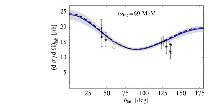
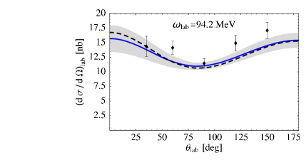
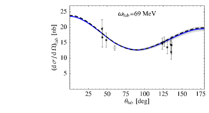
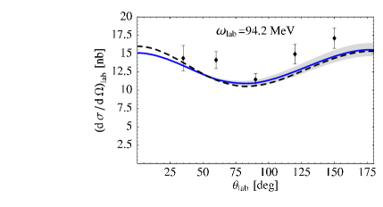
Fig. 9 demonstrates that this compensation works very well in the $\gamma d$ cross sections, as the curves, which correspond to the $\mathcal{O}(\epsilon^{3})$ SSE and to the $\mathcal{O}(\bar{q}^{3})$ HB$\chi$PT fits, are nearly indistinguishable. We consider the quality of our $\mathcal{O}(\bar{q}^{3})$ fit to be comparable to that of the $\mathcal{O}(q^{4})$ fits of Ref. [17].

The SSE and HB$\chi$PT fit results shown in Fig. 9 only differ in the associated pairs $\alpha_{E}$, $\beta_{M}$. Therefore, from the available $\gamma d$ data alone one cannot draw any firm conclusion regarding the importance of explicit $\Delta(1232)$ degrees of freedom. However, as we will show in the next section, from $\gamma p$ scattering experiments it is clear that third-order HB$\chi$PT does not describe the dynamics in the $\gamma d$ process correctly. Given that the SSE calculation describes both the $\gamma p$ and the $\gamma d$ experiments we believe we have established that a Chiral Effective Field Theory which includes the explicit $\Delta$ field is an efficient framework with which to describe low-energy Compton scattering.

4.3 Towards an Unbiased Fitting Procedure

angle [deg]	$\mathrm{d}\sigma/\mathrm{d}\Omega$ [nb]
45.6	$17.3\pm 2.8$
130.5	$14.2\pm 2.1$

Table 3: Effective data points representing the 67 MeV data from [10].

When we compare the several data sets that we use for the fits, we find eleven data points at $\omega_{\mathrm{lab}}\approx 69$ MeV, centered around only two different angles, and five points at $\omega_{\mathrm{lab}}\approx 94.2$ MeV, distributed over the whole angular spectrum. Especially around $\theta_{\mathrm{lab}}\approx 130^{\circ}$ there is a wealth of data around 69 MeV (six points from [10] and one from [9]), which gives an anomalously strong constraint to our fit routines. As long as there are no further data available at higher energies, fitting to all of the 69 MeV data thus overestimates this energy region with respect to the 94.2 MeV data from [11]. Therefore, in the following we compensate for this imbalance of data by replacing the Lund data [10] by two “effective” pseudo-data points (cf. Table 3 and Fig. 11), which represent the data in the forward and backward direction, respectively. These are obtained by weighting the angles and the differential cross section values of the represented data points by the inverse of their errors, and we assign the average over the errors of the represented data as error bars. Therefore, the remaining data are the two data points from [9] at 69 MeV, the two “effective” data at $\sim$67 MeV, shown in Table 3, representing [10], and the five data points from [11] around 94.2 MeV. With these nine data points we perform the same fits as we did before for the complete data sets. The resulting values for $\alpha_{E}$ and $\beta_{M}$ are presented in Table 4, the plots (including the two effective data points) in Fig. 11, exhibiting better agreement with the 94.2 MeV data than the fits of Sect. 4.2 (Fig. 9), as expected. Comparing the results for $\alpha_{E}^{s}$ and $\beta_{M}^{s}$ of Table 4 (or, equivalently, for $\alpha_{E}^{n}$ and $\beta_{M}^{n}$) to the results from our fits to all data points, given in Table 2, we note that both for $\mathcal{O}(\epsilon^{3})$ SSE and $\mathcal{O}(\bar{q}^{3})$ HB$\chi$PT $\alpha_{E}$ is slightly smaller ($\beta_{M}$ slightly larger).

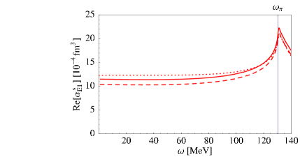
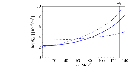
We also see once again that the theory without explicit $\Delta$ degrees of freedom leads to a systematically larger value for $\beta_{M}^{s}$, supporting our hypothesis that the enhancement is due to the insufficient dynamics in the HB$\chi$PT (cf. Table 2). This is demonstrated in Fig. 10, which shows the dynamical isoscalar dipole polarizabilities $\alpha_{E1}^{s}(\omega)$, $\beta_{M1}^{s}(\omega)$, calculated from third-order SSE and HB$\chi$PT, respectively. The static values are taken from the unconstrained fit, using the NNLO $\chi$PT wave function, i.e.

$$\alpha_{E}^{s}=11.5\cdot 10^{-4}\;\mathrm{fm}^{3}\,,\;\;\;\;\beta_{M}^{s}=2.4\cdot 10^{-4}\;\mathrm{fm}^{3}$$ (16)

for the $\mathcal{O}(\epsilon^{3})$ SSE-curve, and

$$\alpha_{E}^{s}=10.4\cdot 10^{-4}\;\mathrm{fm}^{3}\,,\;\;\;\;\beta_{M}^{s}=3.5\cdot 10^{-4}\;\mathrm{fm}^{3}$$ (17)

for the $\mathcal{O}(\bar{q}^{3})$ $\chi$PT-curve. As shown in Fig. 10 the energy dependence of the two field-theoretical calculations for $\alpha_{E1}(\omega)$ is in good agreement with each other and with the recent analysis from Dispersion Theory [2]. Matters are different for $\beta_{M1}(\omega)$: Whereas the SSE-curve reproduces the paramagnetic rise due to the explicitly included $\Delta$ resonance, the HB$\chi$PT result amounts to a nearly energy-independent average for this quantity. However, it is well-known that this paramagnetic rise in the Compton multipoles is necessary for the correct description of the $\gamma p$ data around pion threshold, as can also be seen in the Dispersion-Theory analysis. In HB$\chi$PT the static value is artificially enhanced by the fit constraint from the 94.2 MeV data in order to compensate for the missing dynamics. Both in Fig. 9 and Fig. 11 the enhanced $\beta_{M}$ is able to cure the $\gamma d$ cross sections and make the resulting curves very similar to the plots from the SSE fits (cf. Fig. 11).

Therefore, for understanding the available $\gamma d$ data via fits of $\alpha_{E}^{s}$ and $\beta_{M}^{s}$, it is essential to combine the pairs $\alpha_{E}$, $\beta_{M}$ resulting from the $\gamma d$ analysis with an energy-dependent multipole analysis of $\gamma p$ scattering. From the information available on Compton multipoles from $\gamma p$ scattering experiments, it is clear that third-order HB$\chi$PT is too simplistic a picture for the dynamics of the $\gamma d$ process at energies of $\mathcal{O}(100\;\mathrm{MeV})$. It is therefore crucial that deuteron and proton Compton experiments are available at comparable energies and that they are analyzed within the same framework.

Putting equal statistical weight on the 69 and the 94.2 MeV data can be seen as a demonstration of the importance of obtaining comparable statistics at all energies. We therefore urge for more experimental information at photon energies around 100 MeV. With such information, deuteron Compton cross sections below the pion mass provide an excellent window to investigate which internal nucleonic degrees of freedom contribute in both processes, $\gamma p\rightarrow\gamma p$ and $\gamma d\rightarrow\gamma d$.

Figure 10: Comparison of the isoscalar Dispersion Theory result (dotted) of Ref. [2] for the dynamical dipole polarizabilities $\alpha_{E1}^{s}(\omega)$ and $\beta_{M1}^{s}(\omega)$ to the $\mathcal{O}(\epsilon^{3})$ SSE (solid) and the $\mathcal{O}(\bar{q}^{3})$ HB$\chi$PT (dashed) results with the static values from the two-parameter fit using the chiral wave function, given in Table 4. $\omega_{\pi}$ denotes the pion-production threshold.

Amplitudes	Quantity	2-par. fit	1-par. fit	2-par. fit	1-par. fit
		NNLO $\chi$PT	NNLO $\chi$PT	Nijm93	Nijm93
$\mathcal{O}(\epsilon^{3})$ SSE	$\chi^{2}/d.o.f.$	2.61	2.28	3.72	3.37
	$\alpha_{E}^{s}\;\,[10^{-4}\,\mathrm{fm}^{3}]$	$11.5\pm 1.4$	$11.7\pm 0.8$	$13.6\pm 1.4$	$13.1\pm 0.7$
	$\beta_{M}^{s}\;\,[10^{-4}\,\mathrm{fm}^{3}]$	$2.4\pm 1.7$	$2.8\mp 0.8$	$2.2\pm 1.7$	$1.4\mp 0.7$
	$\alpha_{E}^{s}+\beta_{M}^{s}\;\,[10^{-4}\,\mathrm{fm}^{3}]$	$13.9\pm 2.2$	$14.5\,(\mathrm{fit})$	$15.8\pm 2.2$	$14.5\,(\mathrm{fit})$
	$\alpha_{E}^{n}\;\,[10^{-4}\,\mathrm{fm}^{3}]$	$10.9\pm 1.4$	$11.3\pm 0.9$	$15.1\pm 1.4$	$14.1\pm 0.8$
	$\beta_{M}^{n}\;\,[10^{-4}\,\mathrm{fm}^{3}]$	$3.2\pm 1.7$	$4.0\pm 0.9$	$2.8\pm 1.7$	$1.2\pm 0.8$
$\mathcal{O}(\bar{q}^{3})$ HB$\chi$PT	$\chi^{2}/d.o.f.$	3.14	2.77	4.36	3.93
	$\alpha_{E}^{s}\;\,[10^{-4}\,\mathrm{fm}^{3}]$	$10.4\pm 1.3$	$10.6\pm 0.8$	$12.4\pm 1.3$	$12.0\pm 0.8$
	$\beta_{M}^{s}\;\,[10^{-4}\,\mathrm{fm}^{3}]$	$3.5\pm 1.7$	$3.9\mp 0.8$	$3.3\pm 1.6$	$2.5\mp 0.8$
	$\alpha_{E}^{s}+\beta_{M}^{s}\;\,[10^{-4}\,\mathrm{fm}^{3}]$	$13.9\pm 2.1$	$14.5\,(\mathrm{fit})$	$15.7\pm 2.1$	$14.5\,(\mathrm{fit})$
	$\alpha_{E}^{n}\;\,[10^{-4}\,\mathrm{fm}^{3}]$	$8.7\pm 1.3$	$9.1\pm 0.9$	$12.7\pm 1.3$	$11.9\pm 0.9$
	$\beta_{M}^{n}\;\,[10^{-4}\,\mathrm{fm}^{3}]$	$5.4\pm 1.7$	$6.2\pm 0.9$	$5.0\pm 1.6$	$3.4\pm 0.9$

Table 4: Values for the isoscalar and neutron polarizabilities from a fit to the 69 MeV and 94.2 MeV data sets [9, 11], using the $\mathcal{O}(\epsilon^{3})$ SSE amplitudes and the $\mathcal{O}(\bar{q}^{3})$ HB$\chi$PT amplitudes, respectively. The data from [10] have been replaced by two pseudo-data points, specified in Table 3. The neutron results are derived using the proton values from [3] as input. All error bars displayed are only statistical.

Figure 11: $\mathcal{O}(\epsilon^{3})$ SSE (solid) and $\mathcal{O}(\bar{q}^{3})$ HB$\chi$PT (dashed) results with $\alpha_{E}^{s}$, $\beta_{M}^{s}$ from Table 4, using the chiral NNLO wave function [28]. The upper panels correspond to a fit of both polarizabilities, in the lower panels the Baldin Sum Rule (cf. Eq. (13)) is used as additional fit constraint. The grey bands are derived from our (statistical) errors. The two data points plotted as boxes are the effective data that we use as representative pseudo-data points for the data from [10]. The full set of data points can be seen in Fig. 9.

5 Conclusion and Outlook

In this work Compton scattering from the deuteron was calculated up to next-to-leading order in the Small Scale Expansion, an Effective Field Theory with nucleons, pions and the $\Delta(1232)$ resonance as explicit degrees of freedom. We investigated three different energies and compared to the available experimental data, finding good agreement for 69 MeV and 94.2 MeV and a failure of our calculation for 49 MeV. The reason for this last result is that for low energies our power counting breaks down, so one has to modify the power counting in the very-low-energy region and use non-perturbative methods in order to reproduce the correct low-energy theorems. It will be one of our future projects [30] to get the region $\omega<50$ MeV under control and finally to restore the correct Thomson limit. Here we concentrated on the energy range between 50 MeV and 100 MeV. We found that our calculation gives reasonable results for photon energies above 60 MeV. Motivated by the good agreement at these higher energies, we fitted the isoscalar polarizabilities $\alpha_{E}^{s}$ and $\beta_{M}^{s}$ to the data around 69 MeV and 94.2 MeV, yielding results in good agreement with the $\mathcal{O}(q^{4})$ HB$\chi$PT estimate of Ref. [34] and experiment. Averaging over the results of our two unconstrained SSE fits (one with the chiral NNLO wave function [28], one with the Nijm93 wave function [18], cf. Table 2) results in the isoscalar polarizabilities

$$\alpha_{E}^{s} =(13.2\pm 1.3\,(\mathrm{stat})\pm 2.1\,(\mathrm{syst}))\cdot 10^{-4}\;\mathrm{fm}^{3}\,,$$

$$\beta_{M}^{s} =(1.7\pm 1.6\,(\mathrm{stat})\pm 0.3\,(\mathrm{syst}))\cdot 10^{-4}\;\mathrm{fm}^{3}\,,$$ (18)

where we assumed the same statistical errors as in Table 2. The systematic error due to the differing results when we use different wave functions was estimated to be around 15 %. As these results are in good agreement with the isoscalar Baldin Sum Rule, cf. Eq. (13), we also used the central sum-rule value as additional fit constraint, obtaining

$$\alpha_{E}^{s} =(13.1\pm 0.7\,(\mathrm{stat})\pm 2.0\,(\mathrm{syst}))\cdot 10^{-4}\;\mathrm{fm}^{3}\,,$$

$$\beta_{M}^{s} =(1.5\mp 0.7\,(\mathrm{stat})\pm 0.2\,(\mathrm{syst}))\cdot 10^{-4}\;\mathrm{fm}^{3}\,.$$ (19)

Motivated by the statistical imbalance between experimental data around 94.2 MeV and 69 MeV, we reduced in a second fit the statistics at 69 MeV, replacing the nine data points given in [10] by two representative pseudo-data points, leading to an equal weighting between the two energy sets. The bias-corrected fitting procedure confirms our findings of small values for $\beta_{M}^{s}$, implying small isovector components. Our results for the isoscalar polarizabilities that we derive from the fit including only the two representatives of the data from [10] are

$$\alpha_{E}^{s} =(12.6\pm 1.4\,(\mathrm{stat})\pm 1.9\,(\mathrm{syst}))\cdot 10^{-4}\;\mathrm{fm}^{3}\,,$$

$$\beta_{M}^{s} =(2.3\pm 1.7\,(\mathrm{stat})\pm 0.3\,(\mathrm{syst}))\cdot 10^{-4}\;\mathrm{fm}^{3}\,.$$ (20)

Including the Baldin constraint we get

$$\alpha_{E}^{s} =(12.4\pm 0.8\,(\mathrm{stat})\pm 1.9\,(\mathrm{syst}))\cdot 10^{-4}\;\mathrm{fm}^{3}\,,$$

$$\beta_{M}^{s} =(2.1\mp 0.8\,(\mathrm{stat})\pm 0.3\,(\mathrm{syst}))\cdot 10^{-4}\;\mathrm{fm}^{3}\,.$$ (21)

We consider these “unbiased” results, Eqs. (20) and (21), to be the more reliable values, since in a straightforward fit to the existing $\gamma d$ data there is an obvious imbalance between the number of points at 69 and 94.2 MeV. The data base should be enlarged at higher energies so that unbiased fit results can be obtained. If further experiments, as planned at TUNL/HI$\gamma$S or at MAXlab, provide additional data at energies between 70 MeV and the pion mass over the whole angular range, an unbiased fitting routine including data over this entire energy region will be possible. However, we caution that we found a very strong energy dependence of the $\gamma d$ cross sections in the forward direction. Therefore, we would recommend that any future data taken over a range of photon energies be analyzed using a model which incorporates this rapid energy dependence.

A previous analysis of $\gamma p$ data within the same chiral Effective Field Theory used here yielded the values $\alpha_{E}^{p}=(11.04\pm 1.36)\cdot 10^{-4}\;\mathrm{fm}^{3}$, $\beta_{M}^{p}=(2.76\mp 1.36)\cdot 10^{-4}\;\mathrm{fm}^{3}$ for the proton polarizabilities [2], cf. Eq. (2), which are consistent with experimental values [3]. Combining the numbers of Eq. (20) with these results, we obtain a consistent Effective Field Theory determination of the neutron polarizabilities with a precision comparable to [4]:

$$\alpha_{E}^{n} =(14.2\pm 2.0\,(\mathrm{stat})\pm 1.9\,(\mathrm{syst}))\cdot 10^{-4}\;\mathrm{fm}^{3}\,$$

$$\beta_{M}^{n} =(1.8\pm 2.2\,(\mathrm{stat})\pm 0.3\,(\mathrm{syst}))\cdot 10^{-4}\;\mathrm{fm}^{3}\,$$ (22)

Eq. (22) does not include the Baldin Sum Rule, whereas the one-parameter fit using the Baldin constraint gives

$$\alpha_{E}^{n} =(13.8\pm 1.6\,(\mathrm{stat})\pm 2.1\,(\mathrm{syst}))\cdot 10^{-4}\;\mathrm{fm}^{3}\,,$$

$$\beta_{M}^{n} =(1.4\mp 1.6\,(\mathrm{stat})\pm 0.2\,(\mathrm{syst}))\cdot 10^{-4}\;\mathrm{fm}^{3}\,.$$ (23)

It is clear from Eqs. (2), (22), (23) that the isovectorial components – i.e. the differences between proton and neutron polarizabilities – are rather small. This finding is in good agreement with [4], where quasi-elastic Compton scattering off the proton and neutron was measured. Eqs. (22) and (23) prove that small isovectorial nucleon polarizabilities are not in contradiction with elastic deuteron Compton scattering data. We conclude that both the quasi-elastic and the elastic deuteron Compton experiments are consistent with small isovectorial polarizabilities.

Furthermore we used the $\mathcal{O}(\bar{q}^{3})$ HB$\chi$PT amplitudes for analogous fits, finding similar values for $\alpha_{E}$ but larger ones for $\beta_{M}$, which is not surprising, as the dynamics of the resonant Compton multipoles is not well captured in third-order HB$\chi$PT. Therefore, the static value becomes large, since it must correct for the missing $\Delta$ resonance, leading $\mathcal{O}(\bar{q}^{3})$ HB$\chi$PT to a disagreement with the single-nucleon Compton multipoles extracted in theories with an explicit $\Delta(1232)$, e.g. Ref. [2]. Obviously, $\gamma d$ scattering alone is not sufficient to investigate the relevant low-energy degrees of freedom in nuclear Compton scattering, but one has to combine information from $\gamma d$ and $\gamma p$ scattering and analyze both in the same framework.

Finally, in future work one needs to address the issue of the sensitivity to the wave function (cf. Sect. 3.3), as one would expect that for photon energies below 100 MeV any effects of short distance, i.e. high-energy physics, should be able to be encoded in counter-terms within a well-understood power counting scheme.

References

- [1] H.W. Grießhammer and T.R. Hemmert, Phys. Rev. C 65, 045207 (2002).
- [2] R.P. Hildebrandt, H.W. Grießhammer, T.R. Hemmert and B. Pasquini, Eur. Phys. J. A 20, 293 (2004).
- [3] Olmos de Leon et al., Eur. Phys. J. A 10, 207-215 (2001).
- [4] K. Kossert et al., Eur. Phys. J. A 16, 259 (2003).
- [5] J. Schmiedmayer et al., Phys. Rev. Lett. 66, 1015 (1991).
- [6] T.L. Enik et al., Sov. J. Nucl. Phys. 60, 567 (1997).
- [7] L. Koester et al., Phys. Rev. C 51, 3363 (1995).
- [8] V. Bernard, N. Kaiser, J. Kambor, U.-G. Meißner, Nucl. Phys. B 388, 315 (1992).
- [9] M. Lucas, Ph.D. thesis, University of Illinois (1994).
- [10] M. Lundin et al., Phys. Rev. Lett. 90, 192501 (2003).
- [11] D.L. Hornidge et al., Phys. Rev. Lett. 84, 2334 (2000).
- [12] Haiyan Gao, private communication (2002, 2003).
- [13] Bent Schröder, private communication (2004).
- [14] M.I. Levchuk and A.I. L’vov, Nucl. Phys. A 674, 449 (2000).
- [15] J.J. Karakowski and G.A. Miller, Phys. Rev. C 60, 014001 (1999).
- [16] S.R. Beane, M. Malheiro, D.R. Phillips and U. van Kolck, Nucl. Phys. A 656, 367 (1999).
- [17] S.R. Beane, M. Malheiro, J.A. McGovern, D.R. Phillips and U. van Kolck, Phys. Lett. B 567, 200 (2003) and [nucl-th/0403088].
- [18] V.G. Stoks, R.A. Klomp, C.P. Terheggen and J.J. de Swart, Phys. Rev. C 49, 2950 (1994).
- [19] R. Machleidt, F. Sammarruca and Y. Song, Phys. Rev. C 53, 1483 (1996).
- [20] R.B. Wiringa, V.G. Stoks and R. Schiavilla, Phys. Rev. C 51, 38 (1995).
- [21] S.R. Beane, V. Bernard, E. Epelbaum, U.-G. Meißner and D.R. Phillips, Nucl. Phys. A 720, 399 (2003).
- [22] D.R. Phillips, Phys. Lett. B 567, 12 (2003).
- [23] E. Jenkins and A. Manohar, Phys. Lett. B 259, 353 (1991).
- [24] T.R. Hemmert, B.R. Holstein and J. Kambor, Phys. Lett. B 395, 89 (1997).
- [25] V. Pascalutsa and D.R. Phillips, Phys. Rev. C 67, 055202 (2003).
- [26] V. Bernard, N. Kaiser and U.-G. Meißner, Int. J. Mod. Phys. E 4, 193 (1995).
- [27] T.R. Hemmert, B.R. Holstein, J. Kambor and G. Knöchlein: Phys. Rev. D 57, 5746 (1998).
- [28] E. Epelbaum, W. Glöckle and U.-G. Meissner, Eur. Phys. J. A 19, 125 (2004); ibid. 19, 401 (2004).
- [29] J.L. Friar, Ann. of Phys. 95, 170 (1975).
- [30] R.P. Hildebrandt, H.W. Grießhammer, T.R. Hemmert and D.R. Phillips, in preparation.
- [31] S.R. Beane and M.J. Savage, Nucl. Pys. A 694, 511 (2001); H.W. Grießhammer and G. Rupak, Phys. Lett. B 529, 57 (2002).
- [32] T.R. Hemmert, B.R. Holstein and J. Kambor, J. Phys. G 24, 1831 (1998).
- [33] T.R. Hemmert and B.R. Holstein, in preparation.
- [34] V. Bernard, N. Kaiser, U.-G. Meißner and A. Schmidt, Phys. Lett. B 319, 269 (1993); Z. Phys. A 348, 317 (1994).