Abstract

In this thesis, several color-superconducting phases where quarks of the same flavor form Cooper pairs are investigated. In these phases, a Cooper pair carries total spin one. A systematic classification of theoretically possible phases, discriminated by the color-spin structure of the order parameter and the respective symmetry breaking pattern, is presented. In the weak-coupling limit, i.e., for asymptotically high densities, a universal form of the QCD gap equation is derived, applicable to arbitrary color-superconducting phases. It is applied to several spin-one and spin-zero phases in order to determine their energy gaps and critical temperatures. In some of the spin-one phases the resulting gap function is anisotropic and has point or line nodes. It is shown that the phases with two different gaps violate the well-known BCS relation between the critical temperature and the zero-temperature gap. Moreover, the screening properties of color superconductors regarding gluons and photons are discussed. In particular, it turns out that, contrary to spin-zero color superconductors, spin-one color superconductors exhibit an electromagnetic Meissner effect. This property is proven by symmetry arguments as well as by an explicit calculation of the gluon and photon Meissner masses.

Kapitel 1 Introduction

The first three sections of this thesis serve as a motivation and as an introduction into the basics of the underlying theories that describe the physics. In these introductory sections, we essentially address the following questions. The first question is related to the second term of the thesis’ title, “cold and dense quark matter”. It is, of course, “Why do we study cold and dense quark matter?”. This question naturally is connected with the questions “Where and when (= under which conditions) does cold and dense quark matter exist?” and, simply, but important, “What is cold and dense quark matter?”. The first part of this introduction, Sec. 1.1, is dedicated to these questions, which will be studied without discussing technical details in order to allow an easy understanding of the thesis’ main goals.

The second question addressed in the introduction, namely in Sec. 1.2, is related to the first term of the thesis’ title, more precisely to its third word, “superconductivity”. This question simply is “What is superconductivity?”. Since this is a theoretical thesis, this question basically will turn out to be “What are the theoretical means to explain superconductivity?”. This section is a pure “condensed-matter section”, or more precisely, a “low-energy condensed-matter section”, i.e., we focus on many-particle (= many-fermion) systems adequately described solely by electromagnetic interactions. It introduces the basics of the famous BCS theory, developed in the fifties in order to explain the phenomena and the mechanism of superconductivity in metals and alloys. A special emphasis is put on the theoretical concept of “spontaneous symmetry breaking”, a concept widely and successfully applied to a variety of different fields in physics. Although phenomenologically quite different from superconductors, a second physical system is introduced in Sec. 1.2, namely superfluid Helium 3 (³He). From the theoretical point of view, superfluidity is very similar to superconductivity. Furthermore, the theory of superfluid ³He contains important aspects (not relevant in ordinary superconductivity) which are applicable to color superconductivity, and especially to spin-one color superconductivity.

Therefore, in the last part of the introduction, Sec. 1.3, we approach the question “What is color superconductivity?” by asking “How are color superconductors related to ordinary superconductors and superfluid ³He?”. It turns out that the methods on which the theory of color superconductors is built on, do not differ essentially from the well-established methods introduced in Sec. 1.2. However, we consider quark matter! Therefore, this “condensed-matter physics of QCD” is more than a transfer of well-known theories to a different physical system. Besides the physically completely different implications, which extensively touch the field of astrophysics, also the theory gains complexity due to the complicated nature of quarks and the involved properties of QCD. Of course, Sec. 1.3 also discusses the question “What is special about spin-one color superconductors?”, and, since particularly spin-zero color superconductors have been a matter of study in a large number of publications in recent years, “Why should not only spin-zero, but also spin-one color superconductors be considered?”.

1.1 Cold and dense quark matter

1.1.1 The phase diagram of QCD

In the phase diagram of quantum chromodynamics (QCD), Fig. 1.1, every point represents an infinitely large system of quarks and gluons in thermal equilibrium with a certain temperature $T$ and a quark chemical potential $\mu$. Since the particle number density $\rho$ is a monotonously increasing function with $\mu$, $\rho\sim\mu^{3}$, we can, for the following qualitative and introductory discussion, equivalently use “system with high chemical potential” and “dense system”. We expect that QCD is the suitable theory even for the extreme regions of this phase diagram, namely very hot or very dense systems. Due to a special property of QCD, called asymptotic freedom [1], the coupling between quarks and gluons becomes weaker in the case of a large momentum exchange or in the case of a small mutual distance. Therefore, applying QCD to systems with high temperature and/or large densities, we expect the quarks to be in a deconfined phase [2], contrary to the low temperature/density phase, where they are confined into hadrons.

In recent years, these “extreme” systems have gained more and more attention in experimental as well as in theoretical physics. There are several reasons for this interest. First of all, it is a general experience in physics that the study of systems in extreme regions of the phase diagram (or in extreme energy regions, or with extreme velocities, masses, etc.) often are followed by genuinely new developments in theory and experiment, leading to a deeper understanding of the existing theories (and of nature) or to a completely new theory. Therefore, it is an outstanding goal of research to go beyond temperatures and densities at which quarks are in the ordinary hadronic phase. Simply speaking, take a system of quark matter and heat it up and/or squeeze it to a sufficient amount and you will definitely learn a lot of new physics. Second, the investigation of systems under extreme conditions might help to understand special regions (in space and in time) of the universe. In other words, most likely there exists or existed quark matter in the deconfined phase, also called quark-gluon plasma. For instance, in the early stages of its evolution the universe was very hot. While cooling down, the universe passed through a cross-over into the hadronic phase (note that the quark-hadron phase boundary ends in a critical point; thus, for small densities, as present in the early universe, there is no phase transition in the strict sense from the quark-gluon plasma to the hadronic phase).

Through collisions of heavy nuclei at ultrarelativistic energies one tries to imitate the situation of the early universe in the laboratory [3]. In these experiments, one expects to create a quark-gluon plasma at least for a short time, after which the temporarily deconfined quarks again form hadrons. Since these hadrons are the particles that can be observed by the detectors (and not the individual quarks), it is a subtle task to deduce the properties (or even the existence) of the quark-gluon plasma from the experimental data. Nevertheless, in recent years, a fruitful, though often controversial, interplay between different experimental groups as well as between experiment and theory has led to an established opinion that the quark-gluon plasma can be created in heavy-ion collisions (with bombarding energies experimentally accessible nowadays or in the near future) or that it already has been created. Still, there are a lot of open questions in this field (note for instance, that, in order to describe heavy-ion collisions properly, one needs nonequilibrium methods).

Theoretically, the region of high temperature and low density (strictly speaking, $\mu=0$) can be described by “lattice QCD” [4]. In lattice QCD, one calculates the partition function of thermal QCD numerically on a lattice in the four-dimensional space spanned by the three spatial directions and the inverse temperature axis. Making use of the so-called Polyakov loop (or Wilson line) as an order parameter, lattice QCD is able to make predictions for the nature and the critical temperature of the quark-hadron phase transition [5, 6]. Recently, also the technically involved problem of extending lattice QCD calculations to nonzero chemical potentials has been approached; for a review, see Ref. [7].

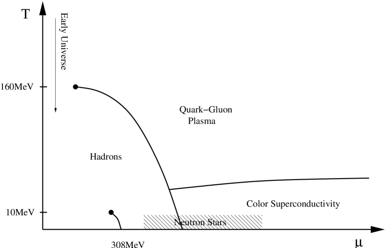
Abbildung 1.1: Schematic view of the QCD phase diagram. The curves indicate the phase boundaries of: the liquid/gas phase transition of nuclear matter, starting at $(T,\mu)=(0,308\,{\rm MeV})$, ending in a critical point at $T=10\,{\rm MeV}$); the hadron-quark phase transition, separating hadronic matter from the quark-gluon plasma and ending in a critical point at $T=160\,{\rm MeV}$; the normal-conducting/superconducting phase transition in the quark-gluon plasma.

Let us now turn to the region of the phase diagram that is of special interest in this thesis, the region of cold and dense matter, named “color superconductivity” in Fig. 1.1. In this plot of the QCD phase diagram, no value of the chemical potential has been assigned to the intersection point of the quark-hadron phase boundary and the $T=0$ axis; unlike the gas-liquid nuclear matter phase transition, which, for $T=0$, occurs at the well-known value $\mu=308\,{\rm MeV}$. The reason for the missing number is simple: One does not know it. This region of the phase diagram, namely cold quark matter at densities ranging from a few times nuclear matter ground state density, $\rho_{0}\sim 0.15\,{\rm fm}^{-3}$, up to infinite density, is poorly understood. Therefore, one (initially theoretical) motivation of this thesis is to contribute to a further understanding of a special region in the QCD phase diagram. The rich phase structure of ordinary condensed-matter physics (one might call it “condensed-matter physics of quantum electrodynamics (QED)”) suggests that also in “condensed-matter physics of QCD” a variety of different phases appears. This connection with ordinary condensed-matter (and solid-state) physics can be considered as another motivation for the study of cold and dense quark matter. On the one hand, both research fields share the interest for similar physical systems, on the other hand, these physical systems differ in essential properties, wherefore it is promising to learn from each other and induce new developments in both fields. This interplay will be illustrated for instance in the next two sections, where color superconductivity (Sec. 1.3) will be based on the theory of ordinary superconductivity and superfluidity (Sec. 1.2).

Another motivation for the investigation of cold and dense matter is its relevance for astrophysics. The densest matter systems have not been produced in the laboratory, they rather exist in nature, namely in compact stellar objects. Therefore, let us insert a short introduction about neutron stars. Elementary introductions about properties and the evolution of neutron stars can be found in text books such as Refs. [8, 9]. For more specialized reviews and articles, treating neutron star properties of special interest for this thesis, see Refs. [10, 11, 12, 13].

1.1.2 Neutron stars

Neutron stars are compact stellar objects that originate from supernova explosions. First observations of neutron stars were done in the late sixties [14]. Neutron stars have a radius of about 10 km and a mass which is of the order of the sun’s mass, $M\sim 0.1M_{S}-2M_{S}$ [9]. Consequently, the matter that a neutron star is composed of is extremely dense; note for a comparison that the sun’s radius is $6.7\cdot 10^{5}\,{\rm km}$. The matter density increases from the surface to the center of the star. Therefore, the matter of a neutron star exists in different phases, each phase forming a layer of the spherical star. At the surface of the neutron star, there is a thin crust of iron, followed by a layer that consists of neutron-rich nuclei in an electron gas. At still higher densities there is a phenomenon called “neutron drip”, i.e., neutrons start to coexist individually in equilibrium with nuclei and electrons. Even closer to the center of the star, approaching nuclear matter density $\rho_{0}$, nuclei cease to exist and a phase of neutrons, protons, and electrons is the preferred state of matter. Neutron stars are called neutron stars because this phase (and the nuclear phase at lower densities) is very neutron-rich. Approaching even higher densities, a phase containing pions, muons, and hyperons is predicted to be the favorite state, i.e., simply speaking, the fundamental elements of neutrons and protons, $u$ and $d$ quarks, start to form different hadrons and also the heavier $s$ quarks might be involved. At the core of the neutron star, matter density might very well reach values an order of magnitude larger than $\rho_{0}$ [9]. Therefore, pure quark matter is likely to be found in the interior of the star.

Properties of neutron stars are explored by theoretical considerations as well as astrophysical observations. Theoretical models make use of two essential ingredients. First, the equation of state, which connects pressure with temperature and energy density. Second, general relativity, i.e., Einstein’s field equations. Experimental data is essentially based on a certain property of a neutron star, namely its rotation. Due to this rotation, neutron stars are pulsars, i.e., they emit electromagnetic radiation in periodic pulses. The rotating periods are in the range of milliseconds [9]. Observations have shown that the spinning-down of the star (the rotation frequency decreases due to radiative energy loss) is interrupted by sudden spin-ups, called glitches.

From the spectra and frequency of the radiation pulses, properties of the neutron star can be deduced. The most important properties, more or less well known, are mass, radius, temperature, and magnetic field of the star. The typical values for mass and radius have been quoted above; let us now briefly discuss temperature and magnetic field. The temperature of neutron stars right after their creation is in the range of $10^{11}\,{\rm K}$, or 10 MeV. During its evolution, the star cools down. This decrease of temperature is dominated by neutrino emission. After a time of about a million years, the star has cooled down to temperatures $\sim 10^{5}\,{\rm K}$, or 10 eV [9, 12]. Consequently, matter in the interior of neutron stars indeed is a realization of “cold and dense matter”, where “cold”, of course, refers to the scale given in the QCD phase diagram, Fig. 1.1. As will be shown in Sec. 2, temperatures present in old neutron stars are certainly lower than the critical temperatures of color superconductors.

Next, let us discuss the magnetic field. Indirect measurements suggest that the magnetic field at the surface of a neutron star is of the order of $10^{12}\,{\rm G}$ [9]. This is thirteen orders of magnitude larger than the magnetic field at the surface of the earth. Many questions concerning the magnetic fields of neutron stars, especially its origin, are not well understood. On the other hand, this physical quantity perhaps is the most important one in order to investigate possible superconducting phases in the interior of the star. Since color superconductivity and its magnetic properties will be a matter of investigation in the main part of this thesis, especially in Sec. 2.3, let us now summarize the conventional picture of a neutron star (= without quark matter) regarding superconductivity and superfluidity. Recent developments in this interesting field can be found in Refs. [10, 13, 15, 16, 17].

As a simplified picture, assume that the neutron star consists of two different phases. One of them containing neutron-rich nuclei and forming the crust of approximately one kilometer. The other one forming the core of the star and consisting of neutrons and protons (and electrons). For sufficiently low temperatures, $T\sim 10^{9}\,{\rm K}$, the neutrons are in a superfluid state while the protons form a superconductor. Therefore, the core of the star is governed by an interplay between a superfluid and a superconductor, both present in the same spatial region. There are at least two observed properties of the star that are closely related to these exotic states in the interior. First, the above mentioned glitches, and second, the precession periods of the star. The explanation of the glitches is closely related to the superfluidity of the neutrons. Due to the rotation of the star, an array of vortex lines is formed. This vortex array expands when the star spins down. Sudden jumps of the rotation frequency are explained by the fact that the vortex lines are pinned to the crust of the star [10]. The picture becomes more complicated if one includes the superconducting protons. If this superconductor is of type-II, there are magnetic flux tubes through which the magnetic field may penetrate the core of the star. Taking into account an interaction between these flux tubes and the superfluid vortices, it has been shown that this picture of a neutron star contradicts the observed precession periods of about one year [16]. In Refs. [15, 17], however, the possibility is pointed out that protons form a type-I superconductor.

At the end of this astrophysical intermezzo, let us also mention that not only conventional neutron stars and neutron stars with a quark core have been studied, but also the possibility of pure quark stars. Recent interpretations of observations regarding this question can be found in Refs. [18].

1.2 Superconductivity and superfluidity

Superconductivity as well as superfluidity are states of interacting many-fermion systems that are distinguished from the normal state by an order parameter. The transition from the normal state to the superconducting or superfluid state therefore is a phase transition. The order parameter characterizes the different phases and, as a function of temperature, changes its value at a certain temperature, the critical temperature $T_{c}$. While this function is zero in the normal phase, it assumes a nonzero value in the superconducting and superfluid phases. The concept of an order parameter and a critical temperature is common to all phase transitions. For instance, in the liquid/gas phase transition of water the order parameter is the particle density, which discontinuously changes from one phase to the other. Another example is ferromagnetism, where the order parameter is given by the magnetization.

In both superconductivity and superfluidity the order parameter is given by a less trivial quantity. Although the mathematical structure of the order parameter can be quite different for superconductors and superfluids (and also for different kinds of these systems), the underlying physical mechanism is the same in each case. This fact allows us to identify the order parameter as the quantity accounting for existence (superconductor/superfluid) or non-existence (normal state) of Cooper pairs. In the following we will elaborate on the properties and theories of superconductors and superfluids. In the case of the latter, we will focus on superfluid ³He. One can find reviews of these theories in many textbooks such as Refs. [19, 20, 21, 22].

1.2.1 Superconductivity

The history of superconductivity started in 1911, when Kamerlingh Onnes discovered that the electric resistance of mercury became unmeasurably small below temperatures of $4.2\,{\rm K}$ [23]. Almost fifty years later, in 1957, a theoretical model for the phenomenon of superconductivity, based on microscopic theories, was published [24]. This theory by Bardeen, Cooper, and Schrieffer (BCS theory) has been very successful in explaining and predicting the properties of conventional superconductors until this day. However, in 1986, with the first discovery of high-$T_{c}$ superconductors [25], a class of superconductors was started to be studied, for which still no satisfactory theoretical explanation has been found. These high-$T_{c}$ superconductors can have transition temperatures up to $125\,{\rm K}$.

As mentioned above, the nonzero value of the order parameter in the superconducting phase is equivalent to the existence of Cooper pairs. Let us explain this in some more detail. The physical system we are dealing with is a metal or alloy. Theoretically, it can be described by an interacting many-electron system in the presence of phonons, i.e., lattice oscillations. Since electrons are fermions, they obey the Pauli exclusion principle and thus, at $T=0$, all quantum states up to a certain energy, the Fermi energy $\epsilon_{F}=\mu$ (where $\mu$ is the electron chemical potential), are occupied, each by a single electron, while all energy states above $\epsilon_{F}$ are empty. In momentum space, due to $\epsilon_{k}^{0}=p^{2}/(2m)$, where $\epsilon_{k}^{0}$ is the energy, $p\equiv\hbar k$ the momentum, and $m$ the mass of the electron, the boundary between occupied and empty states is the surface of a sphere, the Fermi sphere, whose radius is given by the Fermi momentum $p_{F}\equiv\hbar k_{F}$. Cooper showed that if there is an arbitrarily weak attractive force between the fermions, a new ground state of the system will be preferred, in which electrons at the vicinity of the Fermi surface form pairs (comparable to a bound state). Then, the total energy of the system is reduced by the amount of the sum of the binding energies of the electron pairs. Moreover, the single particle excitation energies are modified. They acquire a gap $\phi_{k}$, accounting for the fact that in the superconducting state one needs a finite amount of energy to excite an electron (more precisely, a quasiparticle) at the Fermi surface, which is not the case in the normal state, where an infinitesimally small energy is needed to excite an electron at the Fermi surface (cf. Fig. 1.2).

Abbildung 1.2: Fermionic (quasi)particle dispersion relations for the normal and superconducting phases (nonrelativistic).

Coopers theorem applies to a superconductor since, indeed, and in spite of the repulsive Coulomb interaction, there is an attractive force between the electrons. This is provided by exchange of virtual phonons and was first pointed out by Fröhlich [26]. In a crystal, the phonon energy is bounded by the Debye energy $\hbar\omega_{D}$. Thus, the exchanged momentum is much smaller than $\hbar k_{F}$. Therefore, due to Pauli blocking, only electrons at the vicinity of the Fermi surface, say, in an interval $[k_{F}-q,k_{F}+q]$, where $q\ll k_{F}$ is determined by the Debye energy, can interact via this phonon exchange. This is the reason why superconductivity is a pure Fermi surface phenomenon.

In conventional superconductors, each Cooper pair has a vanishing total spin, $S=0$, as well as a vanishing angular momentum, $L=0$ ($s$-wave). In high-$T_{c}$ superconductors, however, the situation seems to be more complicated. Superconductors with $d$-wave states as well as spin-triplet superconductors, $S=1$, have been found experimentally and studied in theoretical models [27, 28]. But let us continue with the simplest situation of conventional superconductors. In this case, both electrons of a Cooper pair have momenta of equal absolute value but opposite direction. Consequently, the total momentum of a Cooper pair vanishes, which is illustrated in Fig. 1.3. The fact that all Cooper pairs must have the same total momentum can, roughly speaking, be explained by a Bose-Einstein condensation of the pairs. In a Bose-Einstein condensate, a macroscopic number (= proportional to the volume of the system) of bosons are in one quantum state, the ground state. But note that in conventional (weak coupling) superconductors the Cooper pairs are extensively overlapping in space. Therefore, they are far from being considered as separated, well-defined bosons and the picture of Bose-condensed Cooper pairs is questionable. Nevertheless, one speaks of a “condensation of Cooper pairs” to describe the superconducting state. However, in strong-coupling superconductors, where the spatial extension of a Cooper pair might be smaller than the average distance between the electrons, a real Bose-Einstein condensation might set in. The difference between BCS Cooper pairing and a Bose-Einstein condensation of Cooper pairs has been studied for instance in Refs. [29, 30] and, for color superconductivity, in Ref. [31].

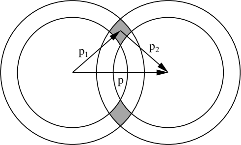
Abbildung 1.3: Schematic picture of the total momentum ${\bf p}$ of an electron Cooper pair, composed of the two electron momenta ${\bf p}_{1}$ and ${\bf p}_{2}$. Only electrons with momenta in a small vicinity around the Fermi surface can form Cooper pairs. Therefore, only electrons in the shaded areas (= volumes in three-dimensional momentum space) can form Cooper pairs with a given momentum ${\bf p}$. The shaded region and thus the total binding energy is maximized for ${\bf p}=0$, i.e., ${\bf p}_{1}=-{\bf p}_{2}$.

Let us now quote the essential equations for a quantitative treatment of superconductivity according to BCS theory. The BCS gap equation for a temperature $T$ and a chemical potential $\mu$ reads [20],

$$1=g\int\frac{d^{3}{\bf k}}{(2\pi)^{3}}\frac{1}{2\epsilon_{k}}\tanh\left(\frac{\epsilon_{k}}{2k_{B}T}\right)\,\,,$$ (1.1)

Here, $k_{B}$ is the Boltzmann constant, $g$ the coupling constant of the attractive electron-electron interaction and $\epsilon_{k}$ the quasiparticle excitation energy (see Fig. 1.2),

$$\epsilon_{k}=\sqrt{(\epsilon_{k}^{0}-\mu)^{2}+\phi^{2}}\,\,.$$ (1.2)

Note that, in order to derive Eq. (1.1), one assumes the interaction to be constant for electrons at the vicinity of the Fermi surface and zero elsewhere. In this case, the gap function $\phi_{k}$ assumes a constant value $\phi$ at the Fermi surface and thus can be cancelled from the original integral equation which leads to Eq. (1.1), where $\phi$ is only present in the excitation energies. Introducing a cut-off for the momentum integration, naturally given by the limit of the phonon energy, $\hbar\omega_{D}$, i.e., integrating solely over the above mentioned momentum interval around the Fermi surface, the gap equation can easily be solved for $T=0$. One obtains

$$\phi=2\hbar\,\omega_{D}\,\exp\left(-\frac{1}{N(0)\,g}\right)\,\,,$$ (1.3)

where

$$N(0)=\frac{m\,k_{F}}{2\pi^{2}\hbar^{2}}$$ (1.4)

is the density of states at the Fermi surface. In the limit $T\to T_{c}$, the gap equation yields a relation between the zero-temperature gap $\phi$ and the critical temperature,

$$\frac{k_{B}T_{c}}{\phi}=\frac{e^{\gamma}}{\pi}\simeq 0.57\,\,,$$ (1.5)

where $\gamma\simeq 0.577$ is the Euler-Mascheroni constant.

The relations given in Eqs. (1.3) and (1.5), regarding the gap parameter and the critical temperature, respectively, are two fundamental results of BCS theory. In the following sections, especially in Sec. 2.1, it will be discussed if and how these results have to be modified for color superconductors.

As discussed in Sec. 1.1.2, it is of great physical importance if a superconductor is of type I or type II. This classification has direct consequences for the behaviour of the superconductor in an external magnetic field. Superconductors of type I are characterized by one critical magnetic field $H_{c}$ (depending on temperature). Therefore, for a fixed temperature and an external magnetic field $H>H_{c}$ the system is in the normal-conducting state, whereas for a magnetic field $H<H_{c}$, the system is in the superconducting state. Moreover, in this case, the superconductor exhibits the Meissner effect, i.e., the magnetic field is expelled from the interior of the superconductor. More precisely, there is a finite penetration length $\lambda$ for the magnetic field, or in other words, the magnetic photon acquires a mass (“Meissner mass”), $m_{M}\sim 1/\lambda$. Superconductors of type II, however, are characterized by two different critical magnetic fields, $H_{c1}<H_{c2}$. For magnetic fields $H>H_{c2}$ the system is in the normal phase, and for $H<H_{c1}$ the system is superconducting with complete expulsion of magnetic fields. For magnetic fields with a strength between the two critical fields, $H_{c1}<H<H_{c2}$, the system is superconducting but the magnetic field penetrates partially into the superconductor through so-called flux tubes. These objects are one-dimensional “topological defects” (= vortices), i.e., tubes with a width of the order of the coherence length $\xi$ where the order parameter or, equivalently, the density of Cooper pairs, vanishes. The type of a superconductor is determined by the Ginzburg-Landau parameter

$$\kappa\equiv\frac{\lambda}{\xi}\,\,.$$ (1.6)

A superconductor is of type I if $\kappa<1/\sqrt{2}$ and of type II if $\kappa>1/\sqrt{2}$. This difference between superconductors with certain values for $\kappa$ and the existence of vortices was theoretically predicted by Abrikosov in 1957 [32], based on the phenomenological Ginzburg-Landau Theory [33]. This prediction turned out to be relevant especially for high-$T_{c}$ superconductors which are of type II and thus show a pattern of flux tubes for suitable external magnetic fields.

1.2.2 Superfluid ³He

Superfluidity in helium was first observed for the isotope ⁴He [34]. Its transition temperature was found to be $T_{c}=2\,{\rm K}$. Since ⁴He atoms are bosons, their superfluid phase is theoretically explained by a Bose-Einstein condensation of the atoms. The lighter isotope ³He, however, is fermionic since it is composed of three nucleons and two electrons, adding up to a non-integer total spin. Motivated by the success of BCS theory, in the sixties, theoreticians applied the mechanism of Cooper pairing to systems with fermionic atoms. Experimentally, superfluid ³He was first observed in 1971 at temperatures around $T_{c}=2\,{\rm mK}$ [35], cf. Fig. 1.4, i.e., three orders of magnitude smaller than in the case of ⁴He. The theoretical breakthrough concerning the explanation of the rich phase structure of superfluid ³He was done by Leggett in 1975 [36].

Abbildung 1.4: Phase diagram for ³He. Two different phases can be found in the superfluid region, namely the A and B phases.

Let us in the following elaborate on some aspects of the theory of superfluid ³He; it will turn out that, in order to understand (spin-one) color superconductivity, it is very useful to be familiar not only with the BCS theory of conventional superconductors but also with the theory of superfluid ³He.

Roughly speaking, superfluidity is the same as superconductivity, with the only difference that the Cooper pairs are not charged. This simplified statement has to be treated with great care (especially in the case of color superconductivity/superfluidity!) and even can be misleading. But nevertheless, let us start with this statement for a brief theoretical introduction into superfluid ³He. Here, as for the electron liquid in metals, there is an attractive interaction between the fermions. This interaction is provided by the van-der-Waals force. Consequently, Cooper’s theorem applies and Cooper pairs of atoms are formed below the transition temperature. These pairs have total momentum ${\bf p}=0$, and there is a gap equation which has a nonzero solution for the gap that occurs in the quasiparticle excitation energies. In this sense, superfluidity is very similar to superconductivity. But since ³He atoms (and thus also the Cooper pairs) are neutral, while electrons carry electric charge, the physical implications are very different for the two systems. The question of electric (and color) neutrality in the case of a color superconductor is much more complicated and will be discussed in Secs. 1.3 and 2.3.

But note another difference between superfluid ³He and conventional superconductors. The atomic interaction potential becomes repulsive for short mutual distances. Therefore, a Cooper pair in ³He has total angular momentum $L=1$ ($p$-wave state), since, in this case, the pair wave function vanishes for zero distance. This has direct implications for the total spin of the pair, as can be seen from the following simple symmetry argument. Since the total wave function of the Cooper pair, consisting of two fermions, has to be antisymmetric and the $p$-wave function is antisymmetric with respect to exchange of the coordinates of the two fermions, it must be symmetric with respect to exchange of the two spin states of the fermions. Thus, in superfluid ³He, the Cooper pairs are in an $S=1$ state. This special feature of a nonzero angular momentum as well as a nonzero spin is the origin for a rich phase structure, i.e., there are several different superfluid phases as can be seen in the phase diagrams shown in Figs. 1.4 and 1.5.

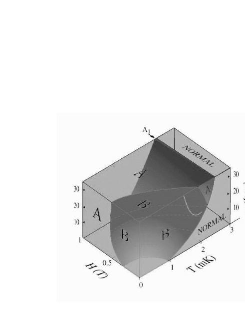
Abbildung 1.5: Phase diagram for ³He including an external magnetic field $H$. For an increasing magnetic field, the B phase becomes more and more disfavored while the A phase covers most of the superfluid region of the phase diagram, and an additional phase, the ${\rm A}_{1}$ phase, that is absent in the situation of a vanishing magnetic field, occurs.

A simple way to understand the occurrence of several different superfluid phases is provided by the concept of spontaneous symmetry breaking. This concept is used in many different fields of physics since it is closely connected with the theory of phase transitions. In order to make use of it in the discussion of color superconductivity, we explain some basic aspects in this introduction and apply them to superfluid ³He.

First, let us discuss the simple example of ferromagnetism. Consider a lattice of localized spins where each spin vector points in a random direction of three-dimensional space, cf. left panel of Fig. 1.6. Then, macroscopically, the system is invariant under arbitrary rotations in real space, i.e., its symmetry group is $G=SO(3)$. This is the non-magnetic phase, where the magnetization, which is the order parameter for this phase transition, vanishes. For temperatures below the critical temperature $T_{c}$, all microscopic spins align in one direction, causing a finite magnetization, cf. right panel of Fig. 1.6. Obviously, the system is no longer invariant under arbitrary rotations. The symmetry is broken. But still, rotations around the axis parallel to the direction of the magnetization do not change the system macroscopically. Therefore, the symmetry is not completely broken, but there is a residual symmetry given by the subgroup $H=U(1)\subseteq G$. The term spontaneous symmetry breaking accounts for the fact that even an infinitesimally small external magnetic field causes the phase transition into the ferromagnetic phase.

Abbildung 1.6: Illustration of the ferromagnetic phase transition. The symmetry is spontaneously broken down from $SO(3)$ (left panel) to $U(1)$ (right panel).

Now we extend our discussion, first on a purely mathematical level, to a symmetry group that is a direct product of two groups $G=U(1)_{a}\times U(1)_{b}$. At this point, let us recall some related group theoretical facts, relevant for various sections of this thesis. All symmetries we are dealing with in this thesis are described by Lie groups or direct products of several Lie groups. Remember that a Lie group is defined as a group that is a differentiable manifold and for which the group operations are continuous. The local structure of the Lie group is determined by the tangent space at the unit element. This vector space is a Lie algebra, i.e., the multiplication in this space is given by the Lie product $[-,-]$ with the usual properties. Since all Lie groups considered in this thesis are matrix groups, $[-,-]$ always is the commutator of two matrices. The basis elements of the Lie algebra are the generators of the Lie group, which means that, via the exponential map, the generators are mapped onto Lie group elements. A direct product of (Lie) groups $G_{1}\times G_{2}$, as in the current example, is again a (Lie) group with group elements $(g_{1},g_{2})$, $g_{1}\in G_{1}$, $g_{2}\in G_{2}$, and the group operation $(g_{1},g_{2})(h_{1},h_{2})=(g_{1}h_{1},g_{2}h_{2})$. Denoting the Lie algebra of $G_{1,2}$ as ${\cal G}_{1,2}$, the Lie algebra of the product group $G_{1}\times G_{2}$ is given by ${\cal G}_{1}\oplus{\cal G}_{2}$. This expression has to be understood as the direct sum of the two vector spaces ${\cal G}_{1}$ and ${\cal G}_{2}$ with the additional property $[A_{1},A_{2}]=0$ for all $A_{1}\in{\cal G}_{1}$, $A_{2}\in{\cal G}_{2}$. Remember also that a subgroup of $G_{1}\times G_{2}$ corresponds to a subalgebra of ${\cal G}_{1}\oplus{\cal G}_{2}$. This correspondence between Lie groups and Lie algebras is used in those sections of this thesis where a detailed discussion of symmetry breaking patterns is presented, see especially Sec. 2.2. In this introduction, let us return to the elementary discussion of symmetry breaking patterns of the group $G=U(1)_{a}\times U(1)_{b}$.

In Fig. 1.7, panel $(i)$ shows a system with a symmetry given by the group $G=U(1)_{a}\times U(1)_{b}$. The solid arrows correspond to $U(1)_{a}$ while the dashed ones correspond to $U(1)_{b}$. More precisely, the system is described by a representation $a\otimes b$ of the group $G$, where $U(1)_{a}$ and $U(1)_{b}$ act on vectors in $a$ (= solid arrows) and vectors in $b$ (= dashed arrows), respectively. In panel $(i)$, arbitrary rotations of both kinds of arrows do not change the macroscopic properties of the system. (Note that, unlike Fig. 1.6, Fig. 1.7 has to be understood as a two-dimensional system; therefore, the rotation group is the one-dimensional $U(1)\cong SO(2)$.) In panel $(ii)$, the symmetry is broken down to the residual subgroup $H=U(1)_{b}$, i.e., the system is still invariant under rotations of the dashed arrows but no longer invariant under rotations of the solid arrows. The corresponding situation with $H=U(1)_{a}$ is represented in panel $(iii)$. In panel $(iv)$, there is no nontrivial subgroup. Any rotation of either of the two classes of arrows changes the macroscopic properties of the system. Thus, the residual group only consists of the unit element, $H=\{{\bf 1}\}$, or, more precisely, $H=\{({\bf 1},{\bf 1})\}$. In this case, the original symmetry is completely broken. The most interesting case is shown in panel $(v)$. A new symmetry arises through the relative orientation of the vectors, the angle between the solid and dashed arrows. Assuming that this microscopic angle corresponds to a macroscopic observable, separate rotation of either solid or dashed arrows changes the system whereas any joint rotation leaves the system invariant. Therefore, we denote the residual symmetry by $H=U(1)_{a+b}$. Mathematically speaking, this subgroup of $G$ is generated by a linear combination of the generators of the original groups $U(1)_{a}$ and $U(1)_{b}$. In the following brief summary of different phases in superfluid ³He it is shown that this symmetry breaking pattern indeed is realized in nature. Another realization can be found in the Weinberg-Salam model of electroweak interactions. And, last but not least, for the study of color superconductivity, cf. for instance Sec. 1.3, it is an essential theoretical ingredient.

Abbildung 1.7: Patterns of symmetry breaking for the case of a direct product group $G=U(1)_{a}\times U(1)_{b}$. Solid arrows correspond to $U(1)_{a}$ while dashed arrows correspond to $U(1)_{b}$.

In the case of superfluid ³He, the symmetry group

$$G=SO(3)_{L}\times SO(3)_{S}\times U(1)_{N}$$ (1.7)

is spontaneously broken. Here, $SO(3)_{L}$ and $SO(3)_{S}$ describe rotations in angular momentum and spin space, respectively, and $U(1)_{N}$ accounts for particle number conservation. The order parameter $\Delta$ is a complex $3\times 3$ matrix since it is an element of the nine-dimensional representation space $[{\bf 3}]_{L}\otimes[{\bf 3}]_{S}$, where $[{\bf 3}]_{L}$ and $[{\bf 3}]_{S}$ are the triplet representations of $SO(3)_{L}$ and $SO(3)_{S}$, respectively. The group $U(1)_{N}$ simply acts via multiplication of a phase factor on this representation. Let us list the order parameters and corresponding residual symmetry groups of the three phases occurring in the phase diagrams in Figs. 1.4 and 1.5.

B phase: $$\Delta_{B}=\frac{1}{\sqrt{3}}\left(\begin{array}[]{ccc}1&0&0\\ 0&1&0\\ 0&0&1\end{array}\right)\,\,,\qquad H_{B}=SO(3)_{L+S}\,\,,$$ (1.8d)

A phase: $$\Delta_{A}=\frac{1}{\sqrt{2}}\left(\begin{array}[]{ccc}0&0&0\\ 0&0&0\\ 1&i&0\end{array}\right)\,\,,\qquad H_{A}=U(1)_{S}\times U(1)_{L+N}\,\,,$$ (1.8h)

$${\rm A}_{1} \Delta_{A_{1}}=\frac{1}{2}\left(\begin{array}[]{ccc}1&i&0\\ -i&1&0\\ 0&0&0\end{array}\right)\,\,,\qquad H_{A_{1}}=U(1)_{S+N}\times U(1)_{L+N}\,\,.$$ phase: (1.8l)

Here and in the following, we use the term “order parameter” somewhat sloppily for the pure matrix (or vector) structure. More rigorously, the order parameter is this matrix multiplied by a gap function, since the order parameter has to be a function that vanishes in the normal phase.

In the B phase, there is a residual group consisting of joint rotations in angular momentum and spin space. Furthermore, the particle number conservation symmetry is completely broken. Note that this phase covers the largest superfluid region of the phase diagram for zero external magnetic field. For a sufficiently large external magnetic field, however, the B phase disappears from the phase diagram. This can be understood from the following symmetry argument. Since an external homogeneous magnetic field, pointing in a constant direction, reduces the original spatial symmetries of the system from arbitrary rotations, $SO(3)$, to rotations around a fixed axis, $U(1)$, there is “no space” for a residual $SO(3)$ as it is present in the B phase. More precisely, in the presence of a magnetic field that reduces the original symmetry, the B phase (and also the A phase) is modified to the so-called ${\rm B}_{2}$ (${\rm A}_{2}$) phase whose residual symmetry is given by $H=U(1)_{L+S}$ ($H=U(1)_{L+N}$).

In the A phase as well as in the ${\rm A}_{1}$ phase, $G$ is broken to a two-dimensional residual subgroup. In both cases, the particle number conservation symmetry couples with the symmetries corresponding to spin and angular momentum. Here, an interesting question arises regarding superfluidity of these phases. Naively speaking, one expects a phase to be superfluid only if $U(1)_{N}$ is broken. In this sense, the B phase in ³He is a superfluid. But how about the A and ${\rm A}_{1}$ phases? Indeed, the superfluidity of these phases in the usual sense is questionable. For instance, in superfluid ⁴He and the B phase in ³He there is a (topologically) stable superflow. This is equivalent to the existence of line defects in the rotating bulk liquid (as already mentioned for superfluid neutron matter in neutron stars, cf. Sec. 1.1.2). This superflow is unstable in the A phase and only becomes stable in the presence of a magnetic field. We do not elaborate further on this point (for more details regarding this interesting problem, see Refs. [22, 37]) but, since in color superconductivity one encounters similar problems, we emphasize that the coupling of the $U(1)_{N}$ symmetry with other symmetries is the origin of nontrivial properties regarding superfluidity.

Finally, we mention one more interesting feature of superfluid ³He, namely the anisotropy of the gap function. As can be seen from Eq. (1.3), for conventional superconductors the gap function is constant on the Fermi sphere. Of course, this is not necessarily valid in cases where the order parameter breaks the rotational symmetry of the system. Therefore, in some phases of superfluid ³He, the gap function $\phi_{k}$ depends on the direction of the fermion momentum $\hbar{\bf k}$. In Fig. 1.8 we schematically show this dependence for the three phases mentioned above.

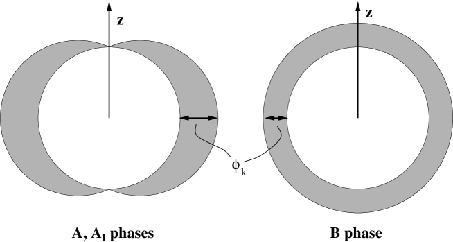
Abbildung 1.8: Angular dependence (schematic) of the gap functions $\phi_{k}$ in the A, ${\rm A}_{1}$, and B phases of superfluid ³He. Both plotted functions are symmetric with respect to rotations around the $z$-axis.

The gap in the B phase is isotropic, while in both other phases there is an anisotropy. Moreover, in the A phase as well as in the ${\rm A}_{1}$ phase, the gap function has nodal points at the north and south pole of the Fermi surface. Consequently, quasiparticles at the Fermi surface whose momentum points into a certain direction (parallel or antiparallel to the $z$-axis) can be excited by an infinitesimally small energy. Therefore, the nodal structure of the gap function is of physical relevance. For instance, the temperature dependence of the specific heat is different in the A phase compared to the B phase (power-law dependence versus exponential dependence). Again, for more details we refer the reader to the special condensed-matter literature [22, 38].

Let us now, being well-prepared by low-energy condensed-matter physics, turn to high-energy condensed-matter physics, i.e., color superconductivity.

1.3 Color superconductivity

In order to provide a plain introduction into the theory of color superconductors (reviews about color superconductivity can be found in Refs. [39, 40, 41, 42, 43, 44]), we connect the physics presented in the previous two sections of this introduction: The theoretical models describing ordinary superconductivity and superfluidity, Sec. 1.2, are applied to cold and dense (= deconfined) quark matter, Sec. 1.1. Since this transfer implies the inclusion of the theory of strong interactions, QCD, and the transition from a nonrelativistic to a relativistic treatment, it is not surprising that a lot of new questions arise in the case of dense quark systems. Nevertheless, the basic mechanism, i.e., Cooper’s theorem, explained in Sec. 1.2.1, can be directly applied. All one has to do is to replace the electron liquid, interacting via exchange of virtual phonons, by a quark system interacting via the strong interaction (thus, no lattice is required for color superconductivity). Due to asymptotic freedom, the strong interaction at (asymptotically) high densities is dominated by the exchange of a single gluon. And indeed, there is an attractive channel of this interaction, providing the condition for the application of Cooper’s theorem. Consequently, for sufficiently low temperatures, the quarks at their Fermi surface rearrange in order to form a ground state characterized by the existence of quark Cooper pairs [45, 46, 47, 48]. Note that, unlike the case of electrons, it is not a priori clear that two quarks, possibly distinguished by their flavor, their color, and their electric charges have identical Fermi momenta. We comment on this question below and first assume that in this respect they behave like electrons in a conventional superconductor.

Then, analogous to a conventional superconductor, in a color superconductor the quarks in the vicinity of the Fermi surface form Cooper pairs with zero total momentum and acquire an energy gap in their (quasiparticle) excitation spectrum. But, considering the different intrinsic properties of quarks compared to electrons, such as flavor, color, and electric charge, the following natural questions arise. Are quark Cooper pairs charged? What is the total spin of a Cooper pair? Is there a Meissner effect in a color superconductor? Are color superconductors also electromagnetic superconductors? How does the quasiparticle dispersion relation look like? How about superfluidity in a color superconductor? Are there vortices/flux tubes? Is a color superconductor of type I or II?

It turns out that color superconductors provide a multitude of theoretically possible phases, and the answers to almost all of the above questions depend on the specific phase and especially on the number of quark flavors $N_{f}$ involved in the system. Therefore, in the following, we briefly discuss several different phases in color superconductors. Common to all phases is the attractive color channel $[\bar{\bf 3}]_{c}^{a}$,

$$[{\bf 3}]_{c}\otimes[{\bf 3}]_{c}=[\bar{\bf 3}]_{c}^{a}\oplus[{\bf 6}]_{c}^{s}\,\,,$$ (1.9)

where the lower index “$c$” indicates “color”, and the upper indices “$a$” and “$s$” stand for “antisymmetric” and “symmetric”, respectively. In this equation, the coupling of two quarks forming a Cooper pair is described with the help of representation theory. The complex vector space on the right-hand side of the equation is nine-dimensional, since each single-quark space $[{\bf 3}]_{c}$ accounts for three fundamental colors, say red, green, and blue. The tensor product can be decomposed into a direct sum of two representations of the color gauge group $SU(3)_{c}$. This is shown on the right hand side of the equation, where the antisymmetric antitriplet $[\bar{\bf 3}]_{c}^{a}$ and the symmetric sextet $[{\bf 6}]_{c}^{s}$ are three- and six-dimensional representations of $SU(3)_{c}$, respectively. (Remember the analogous ansatz for mesons, composed of $u$, $d$, and $s$ quarks and the corresponding antiquarks, $[{\bf 3}]\otimes[\bar{\bf 3}]$, or for baryons, composed of three $u$, $d$, and $s$ quarks $[{\bf 3}]\otimes[{\bf 3}]\otimes[{\bf 3}]$, resulting in the well-known multiplets.) The antisymmetry of the attractive color channel implies that a quark Cooper pair always is composed of two quarks with different colors.

In order to proceed, one has to specify the number of flavors.

1.3.1 Two- and three-flavor color superconductors

Let us first consider the simplest case, a system of massless $u$ and $d$ quarks, i.e., $N_{f}=2$ [46]. According to the number of flavors, the superconducting phase in this system is commonly called the “2SC phase”. In this phase, besides the color antitriplet, Cooper pairs are formed in the flavor-singlet $[{\bf 1}]_{f}^{a}$ and spin-singlet $[{\bf 1}]_{J}^{a}$ channels. While the former is a representation of the flavor group $SU(2)_{f}$ (more precisely, of both the left-handed and right-handed chirality groups $SU(2)_{\ell}$ and $SU(2)_{r}$), the latter is a representation of the spin group $SU(2)_{J}$. Note that in relativistic theories one has to consider the total spin $J=L+S$ rather than separately treating angular momentum $L$ and spin $S$. This is in contrast to the nonrelativistic treatment of superfluid ³He, presented in the previous section. Since both $[{\bf 1}]_{f}^{a}$, $[{\bf 1}]_{J}^{a}$, as well as the color representation $[\bar{\bf 3}]_{c}^{a}$, are antisymmetric with respect to exchange of the corresponding quantum numbers of the single quarks, the total wave function of the quark Cooper pair is antisymmetric, as required by the Pauli principle. Mathematically speaking, a quark Cooper pair in the 2SC phase is an element of the space $[\bar{\bf 3}]_{c}^{a}\otimes[{\bf 1}]_{f}^{a}\otimes[{\bf 1}]_{J}^{a}\cong[\bar{\bf 3}]_{c}^{a}$. Therefore, the order parameter $\Delta$, which, as explained in Sec. 1.2, directly connects the existence of Cooper pairs with a spontaneous breakdown of symmetries, is a complex 3-vector. It is easy to show that, for $N_{f}=2$, any choice of $\Delta$ leads to an equivalent symmetry breaking pattern. For simplicity, one chooses $\Delta_{i}=\delta_{i3}$. The original symmetry of the system,

$$G=SU(3)_{c}\times SU(2)_{f}\times SU(2)_{J}\times U(1)_{em}\times U(1)_{B}\,\,,$$ (1.10)

is broken to

$$H_{2SC}=SU(2)_{c}\times SU(2)_{f}\times SU(2)_{J}\times U(1)_{c+em}\times U(1)_{em+B}\,\,,$$ (1.11)

where $U(1)_{em}$ is the electromagnetic gauge group and $U(1)_{B}$ the baryon number conservation symmetry. Consequently, in the 2SC phase, the flavor and spin groups remain unbroken. However, the color gauge group is broken down to $SU(2)_{c}$. Furthermore, there are two residual $U(1)$’s. The notation for these $U(1)$’s in Eq. (1.11) is explained in Sec. 1.2.2, see Fig. 1.7 and Eqs. (1.8), i.e., $U(1)_{c+em}$ is generated by a linear combination of the generators of $SU(3)_{c}$ and $U(1)_{em}$. Physically, in the 2SC phase, a Cooper pair carries spin zero, $J=0$, it is composed of a $u$ and a $d$ quark, and it carries anti-blue (= anti-3) color charge, since it is composed of a red and a green quark (using the above convention for the order parameter). As can be seen from the residual symmetry group $H_{2SC}$, the question of the electric charge of a Cooper pair is more subtle. It will be discussed in the following section, Sec. 1.3.2. Nevertheless, let us already mention the fundamental differences between the symmetry groups in Eqs. (1.10) and (1.11) compared to the corresponding symmetry breaking patterns in ³He, Eqs. (1.8). While in the latter case, all groups correspond to global symmetries, here two local gauge groups are involved, accounting for the strong and the electromagnetic interaction. Note that in ordinary superconductors, the local group $U(1)_{em}$ is completely broken, whereas the occurrence of the $U(1)_{em}$ generator in the residual group of the 2SC phase demands a careful interpretation (cf. Sec. 1.3.2). Similarly, due to the residual subgroup $U(1)_{em+B}$, the 2SC phase is not superfluid in the usual sense; cf. discussion below Eqs. (1.8) about the A and ${\rm A}_{1}$ phases of superfluid ³He.

Next, we consider a system of three massless quark flavors, $N_{f}=3$. As in the 2SC phase, the condensation of Cooper pairs occurs in the antisymmetric flavor and spin channels, which, together with the antisymmetric color channel, ensures the antisymmetry of the pair wave function. The only difference, caused by the different number of flavors, is the fact that the antisymmetric flavor representation of $SU(3)_{f}$ is an antitriplet (instead of a singlet in the case of $SU(2)_{f}$). Therefore, the order parameter in three-flavor color superconductors is an element of $[\bar{\bf 3}]_{c}^{a}\otimes[\bar{\bf 3}]_{f}^{a}\otimes[{\bf 1}]_{J}^{a}\cong[\bar{\bf 3}]_{c}^{a}\otimes[\bar{\bf 3}]_{f}^{a}$. Consequently, unlike the two-flavor case, the order parameter $\Delta$ is a complex $3\times 3$ matrix. As discussed for the case of superfluid ³He, this structure of the order parameter allows for several different phases. However, in the case of three-flavor color superconductors, it is generally believed that the only important phase is the so-called color-flavor-locked (CFL) phase with an order parameter $\Delta_{ij}=\delta_{ij}$ [49, 50]. In this phase, the symmetry given by the group $G$ in Eq. (1.10) is spontaneously broken to

$$H_{CFL}=SU(3)_{c+f}\times U(1)_{c+em}\,\,.$$ (1.12)

Since not obvious in our simplified notation, it should be mentioned that the order parameter in the CFL phase breaks chiral symmetry in the form $SU(3)_{c}\times SU(3)_{\ell}\times SU(3)_{r}\to SU(3)_{c+\ell+r}$ (in contrast to the 2SC phase, where $SU(2)_{\ell}\times SU(2)_{r}$ is unbroken). In the CFL phase, the order parameter is invariant under joint rotations in color and flavor space. This, of course, is the reason for the term “color-flavor locking”. Furthermore, as in the 2SC phase, there is a local residual $U(1)$ originating from both the color and electromagnetic gauge groups. And, unlike the 2SC phase, $U(1)_{B}$ is completely broken, which renders this phase superfluid.

Let us now elaborate on the physical meaning of the residual gauge group $U(1)_{c+em}$, occurring in both the 2SC and CFL phases.

1.3.2 Anderson-Higgs mechanism in color superconductors

In this section, we point out a certain aspect of spontaneous symmetry breaking, which is relevant for broken gauge symmetries. In conventional superconductors, the electromagnetic gauge symmetry is broken by the order parameter. As mentioned in Sec. 1.2.1, this leads to the Meissner effect, or, equivalently, to a massive photon. This photon mass is generated by the so-called Anderson-Higgs mechanism [51, 52], which is a general mechanism occurring in theories with spontaneously broken gauge symmetries. In color superconductivity, not only the electromagnetic, but also the color gauge group is involved. Let us first briefly introduce the mechanism in a general way. Then, applying it to cold and dense quark matter, we make use of the analogy between the Weinberg-Salam model of electroweak interactions [53] and the two- and three-flavor phases of color superconductivity.

Remember the following basics of spontaneous symmetry breaking in field theories [54]. Consider a Lagrangian for a complex field $\phi\in V$, where $V$ is an $r$-dimensional representation of a Lie group $G$. Suppose that this Lagrangian is invariant under global transformations in $G$. Furthermore, suppose that there is a nonzero ground state of the system (= lowest energy solution of the corresponding equations of motion) $\phi_{0}$ which is invariant under transformations of a subgroup $H$ of $G$, but not under all transformations in $G$. In this case, the symmetry of the system is said to be spontaneously broken and there are ${\rm dim}\,G/H={\rm dim}\,G-{\rm dim}\,H$ massless “Goldstone bosons”, i.e., the originally $r$ degrees of freedom of the matter field generate ${\rm dim}\,G/H$ massless and $r-{\rm dim}\,G/H$ massive modes (present in the vicinity of the vacuum state, i.e., for low energies). Obviously, $r-{\rm dim}\,G/H>0$ is a restriction for possible residual groups $H$. Here, the dimension of a Lie group is defined as the dimension of its Lie algebra.

Now let us gauge the Lagrangian. This is done by introducing a covariant derivative containing gauge fields $A_{a}$, $a=1,\ldots,{\rm dim}\,G$. Then, the Lagrangian is invariant under local transformations of the group $G$; and besides the $r$ degrees of freedom of the field $\phi$, there are $2\,{\rm dim}\,G$ (2 for each massless gauge field) additional degrees of freedom. In this case, spontaneous symmetry breaking caused by a nonzero value of the ground state expectation value creates $r-{\rm dim}\,G/H$ massive modes, as in the non-gauged case. But, instead of the Goldstone bosons there are now ${\rm dim}\,G/H$ massive gauge fields, leaving only the remaining ${\rm dim}\,H$ gauge fields massless. In other words, the degrees of freedom of the “would-be” Goldstone bosons are absorbed (“eaten up”) by the gauge fields which acquire a third degree of freedom and thus become massive. This generation of masses for the gauge fields by spontaneuos symmetry breaking is called Anderson-Higgs mechanism. It was first introduced by Anderson in solid-state physics [51] and then applied by Higgs [52], and later by Weinberg and Salam in particle physics, especially in the theory of electroweak interactions [53].

In the Weinberg-Salam model, the Higgs field is introduced in order to generate the masses of the electron, as well as for the $W^{\pm}$ and $Z$ gauge bosons, since explicit mass terms in the Lagrangian would violate gauge invariance. Let us focus on the gauge fields in this model. The gauge group is $G=SU(2)_{I}\times U(1)_{Y}$ (corresponding to isospin and hypercharge); since ${\rm dim}\,G=3+1=4$, there are originally four massless gauge fields, say $W_{1}$, $W_{2}$, $W_{3}$ for $SU(2)_{I}$, and $W_{0}$ for $U(1)_{Y}$. The vacuum expectation value of the Higgs field, however, is only invariant under $H=U(1)_{I+Y}$, which is generated by a linear combination of one generator of $SU(2)_{I}$ and one of $U(1)_{Y}$. Therefore, there are ${\rm dim}\,G/H=3$ massive gauge fields, called $W^{+}$, $W^{-}$, and $Z$, and ${\rm dim}\,H=1$ massless field $A$. Since the residual group $U(1)_{I+Y}$ contains joint rotations of the original two groups $SU(2)_{I}$ and $U(1)_{Y}$, the pair of fields $(Z,A)$ is generated by an orthogonal rotation of the original pair $(W_{3},W_{0})$. The angle $\theta_{W}$ of the rotation is called Weinberg angle. The resulting fields are the gauge bosons of the weak interaction and the photon field $A$; the residual group is the gauge group of electromagnetism, $U(1)_{I+Y}\equiv U(1)_{em}$. Furthermore, the electromagnetic coupling constant is determined by the coupling constants of the original theory and the Weinberg angle. These facts are summarized in the first column of Table 1.1.

	Weinberg-Salam	CFL phase
gauge	$SU(2)_{I}\times U(1)_{Y}$	$SU(3)_{c}\times U(1)_{em}$
group	isospin, hypercharge	color, electromagnetism
gauge fields	$W_{1},W_{2},W_{3},W_{0}$	$A_{1},\ldots,A_{8},A$
coupling constants	$G$, $G^{\prime}$	$g$, $e$
symmetry	$SU(2)_{I}\times U(1)_{Y}$	$SU(3)_{c}\times U(1)_{em}$
breaking	$\to U(1)_{em}$	$\to U(1)_{c+em}$
	$W^{+},W^{-}$	$A_{1},\ldots,A_{7}$
new fields	$Z=\cos\theta_{W}W_{3}+\sin\theta_{W}W_{0}$	$\tilde{A}_{8}=\cos\theta A_{8}+\sin\theta A$
	$A=-\sin\theta_{W}W_{3}+\cos\theta_{W}W_{0}$	$\tilde{A}=-\sin\theta A_{8}+\cos\theta A$
new coupling constant	$e=G^{\prime}\cos\theta_{W}$	$\tilde{e}=e\cos\theta$
massive fields	$W^{+}$, $W^{-}$, $Z$	$A_{1},\ldots,A_{7},\tilde{A}_{8}$
massless fields	$A$	$\tilde{A}$

Tabelle 1.1: Analogy between the Weinberg-Salam model of electroweak interaction and the CFL phase in a three-flavor color superconductor. In both cases there is a mixing between the original gauge fields. In the case of the CFL phases, all gluons acquire a mass via the Anderson-Higgs mechanism (= color Meissner effect), while the (rotated) photon remains massless (= no electromagnetic Meissner effect).

The second column of Table 1.1 shows the analogous situation in a three-flavor color superconductor. Since the mechanism is exactly the same (the role of the nonvanishing vacuum expectation value of the Higgs field is played by the order parameter of the superconducting state), no further explanation is needed. Physically, one finds that the eighth gluon $A_{8}$ couples to the photon $A$, giving rise to a new (rotated) eighth gluon $\tilde{A}_{8}$ and a new (rotated) photon $\tilde{A}$ [55, 56, 57, 58]. While all original gluons $A_{1},\ldots,A_{7}$ and the new gluon $\tilde{A}_{8}$ acquire a mass via the Anderson-Higgs mechanism, the new photon $\tilde{A}$ remains massless. Consequently, there is a color Meissner effect for all gluons, i.e., color magnetic fields are expelled from the CFL color superconductor. But there is no electromagnetic Meissner effect in the CFL phase, which means that this color superconductor is no electromagnetic superconductor. One should emphasize that the original photon field $A$ has no physical meaning in the interior of the superconductor. The real fields are the rotated fields. This, although at first sight peculiar, can again be understood with the analogous statement in the standard model. In this case, below the “electroweak phase transition”, only the gauge bosons $W^{\pm}$, $Z$, and $A$ are relevant, while the gauge fields of the original symmetry are not existent. Due to the huge difference of the strong and electromagnetic coupling constants, the mixing angle in a color superconductor is small. Therefore, one can interpret the absence of the electromagnetic Meissner effect as follows. An incoming photon is not absorbed at the surface of the superconductor (as in the case of a Meissner effect) but slightly rotated into a new photon that can penetrate the superconductor and thus create a magnetic field in the interior.

The situation in the 2SC phase is very similar. While, for exactly the same reason as in the CFL phase, there is no electromagnetic Meissner effect either, the only difference is the residual color group $SU(2)_{c}$, cf. Eq. (1.11). Therefore, only five gluons become massive, whereas the three remaining ones can penetrate the superconductor. These three massless gluons are those that do not see the third color (remember that all Cooper pairs in the 2SC phase carry (anti-)blue color charge).

A more detailed and quantitative discussion of the Meissner effect (and the Meissner masses) as well as the extension to one-flavor color superconductors are presented in Sec. 2.3.

1.3.3 One-flavor color superconductors

The apparently most trivial situation in cold and dense quark matter is a system with only one quark flavor, $N_{f}=1$. But in this case, a complication enters the color-superconducting phase for the following reason. Due to the antisymmetry of the attractive color channel, cf. Eq. (1.9), the Cooper pair condensation in a one-flavor system has to occur in a symmetric spin channel. Note that in a two- or three-flavor system, the antisymmetric spin channel where the Cooper pairs carry spin zero can be chosen because an antisymmetric flavor channel is available to make the total pair wave function antisymmetric. This is not the case for only one quark flavor. Therefore, in the simplest case, a Cooper pair here carries total spin one, $J=1$, and the order parameter $\Delta$ is an element of $[\bar{\bf 3}]_{c}^{a}\otimes[{\bf 3}]_{J}^{s}$, which is a representation of $SU(3)_{c}\times SU(2)_{J}$. Since integer spin representations are not only representations of $SU(2)_{J}$ but also of $SO(3)_{J}$, we could equivalently choose the symmetry group $SU(3)_{c}\times SO(3)_{J}$. (The groups $SU(2)$ and $SO(3)$ have the same Lie algebra, i.e., they are locally isomorphic, however, globally, they are not isomorphic.) As in the three-flavor case and the case of superfluid ³He, $\Delta$ is a complex $3\times 3$ matrix. Unlike the color-superconducting phases discussed in the previous sections, here the order parameter potentially breaks rotational symmetry in real space. Thus, as in superfluid ³He, anisotropy effects are expected.

Spin-one (or one-flavor) color superconductivity was first studied in Ref. [46]. More recent works discussing spin-one phases can be found in Refs. [59, 60, 61, 62, 63, 64]. In the main part of this thesis, Sec. 2, we study the properties of several possible spin-one color superconducting phases, i.e., we discuss their gap functions, their gap parameters, and their critical temperatures. Moreover, we discuss their response to electric and magnetic fields; in particular, we answer the question if spin-one color superconductors exhibit an electromagnetic Meissner effect. Finally, we study the effective potential in order to determine the preferred phase in a spin-one color superconductor.

1.3.4 More on (color) superconductors

In the previous three introductory subsections about color superconductivity, we focussed on the symmetry aspects of the superconducting phases with $N_{f}=1,2,3$ and pointed out the similarities and differences to ordinary superconductivity and superfluid ³He. In this section, a brief introduction into color-superconducting phases beyond the (idealized) 2SC and CFL phases is given. Most of these phases are not treated in the main part of this thesis, wherefore we cite some useful references. For the investigation of these phases, properties of realistic physical systems, especially of neutron stars, are implemented into the theory of color superconductors. This leads to superconducting phases which are not or only partially based on the traditional BCS theory. Some of these phases have their analogues in ordinary condensed-matter physics. Finally, the following discussion of realistic systems leads to an argument why spin-one color superconductors might be relevant in nature.

It is essential to notice that the above introduced 2SC and CFL phases are based on one fundamental assumption. This assumption is the identity of the Fermi momenta of all $N_{f}$ quark flavors. In conventional superconductors this assumption is valid, since both constituents of a Cooper pair are electrons with identical properties, especially with identical mass and chemical potential, and hence with identical Fermi momenta. Also in superfluid ³He, one expects one single spherical Fermi surface for all helium atoms. Nevertheless, even in conventional condensed-matter physics, this ideal scenario does not always seem to be an appropriate description of the system. There might be two (or more) species of particles having different Fermi surfaces. For instance, in an external magnetic field, due to Zeeman splitting, the electron energy depends on the spin projection and consequently there are two different Fermi momenta for spin-up and spin-down electrons. In this case, a superconducting state may be formed in which the Cooper pairs carry nonzero total momentum, leading to a spatially varying order parameter. This state (FFLO state) was already theoretically predicted in 1964 [65]; experimental evidence for the existence of the FFLO state has been discussed recently [66]. The FFLO state can be understood as a displacement of the Fermi spheres, breaking translational invariance.

Note that a splitting of the Fermi momenta does not necessarily have to originate from an external magnetic field, it might as well be caused by different densities or masses of two fermion species. Besides the formation of Cooper pairs with nonzero momentum, theoretical studies have discussed the possibility of a so-called “interior gap” (or “breached pair”) for systems with two different Fermi momenta [67]. In this case, the fermions with smaller Fermi momentum have to be lifted to a higher energy in order to form Cooper pairs with the fermions with larger Fermi momentum. If this energy cost is lower than the energy gain of the formation of Cooper pairs, the superconducting state is preferred.

Not only for electrons in a metal, but also in atomic systems, the situation of a splitting of Fermi surfaces is investigated [68]. Experiments with ⁶Li and ⁴⁰K (here, the splitting of Fermi surfaces also originates from the spin projections of the atoms) seem to suggest the observation of a superfluid state in a magnetic trap [69, 70]. (Note that these experiments are similar to the celebrated experiments with bosonic atoms where Bose-Einstein condensation of atoms in a magnetic trap has been observed.)

In cold and dense quark matter, it is not surprising that, considering realistic systems, there might be a separation of Fermi surfaces for different quarks. Since quarks carry flavor, color, and electric charge, (and a mass), there are a priori enough intrinsic properties to account for more than one single Fermi momentum. These intrinsic properties have to be combined with the macroscopic properties of realistic systems, such as neutron stars. One of these properties is the overall electric charge neutrality. A second one is the condition of $\beta$-equilibrium (including electrons into the system). Both requirements are implemented in color superconducting quark systems for instance in Refs. [71, 72, 73, 74, 75, 76, 77, 78, 79]. Another complication arises when one relaxes the assumption of ultrarelativistic quarks. In realistic systems, one at least has to take into account the mass difference between the two light $u$ and $d$ quarks and the heavier $s$ quark. (Assuming that $0\simeq m_{u}=m_{d}\ll m_{s}$, the three quark Fermi momenta are given by $k_{F,u}=\mu_{u}$, $k_{F,d}=\mu_{d}$, and $k_{F,s}=\sqrt{\mu_{s}^{2}-m_{s}^{2}}$, where $\mu_{u}$, $\mu_{d}$, and $\mu_{s}$ are the corresponding chemical potentials.) In principle, also the condition of overall color neutrality has to be included. This is done in model calculations via introducing color chemical potentials $\mu_{3}$ and $\mu_{8}$ (cf. for instance Refs. [77, 78, 80]). However, for QCD calculations, it has been shown that color neutrality in a (two-flavor) color superconductor is automatically ensured via a nonvanishing color background field [81, 82].

Anyhow, the question arises if, in spite of the difference between the Fermi momenta of different quark flavors, the superconducting phase is still favored. For color superconductors, there have been suggestions for possible scenarios similar to the ones for electrons or atoms mentioned above. For instance, the FFLO phase is discussed in Refs. [83, 84] (therein called LOFF phase). Besides the deplacement of the Fermi surface in the LOFF phase, also a deformation of the Fermi surfaces, breaking rotational invariance, has been proposed [85]. An interior gap structure is studied in Ref. [86]. The mechanism of breached pairing in a two-flavor color superconductor leads to an interesting phase, called the “gapless 2SC” phase [87] which also has been applied to neutron stars [88]. (Recently, also the possibility of a gapless CFL phase has been investigated [89, 90].) In this phase, a difference (if not too large) between the Fermi momenta of $u$ and $d$ quarks, leads to quasiparticle spectra, which, although exhibiting a nonzero gap parameter $\phi$, for certain quasiparticle momenta look like the normal spectrum, i.e., the spectrum is “gapless”. Note the topological difference between this situation and the nodal structure of the gap in the A phase of superfluid ³He, cf. Fig. 1.8. In the latter, the vanishing gap leads to a gapless excitation energy for quasiparticles with two certain directions of the momentum ${\bf k}$ (but with $|{\bf k}|=k_{F}$). Sloppily speaking, there are two gapless points on the Fermi surface. In the gapless 2SC phase, however, there are two values of $|{\bf k}|$ between the original two Fermi momenta, for which the spectrum becomes gapless. Consequently, there are two gapless spherical surfaces. In the discussion of spin-one color superconductors, we also encounter the situation of gapless lines on the Fermi surface, cf. Sec. 2.1.

It should be mentioned that the values of crucial quantities such as the quark density in the interior of a neutron star, the strange quark mass or the strong coupling constant at moderate (= not asymptotically large) densities are poorly known. Since all these quantities enter the description of the difference in Fermi momenta, the quantitative value of this difference is absolutely unclear. It is easy to understand that there is a limit value for this difference, above which the superconducting state, with Cooper pairs formed by fermions with different Fermi momenta, is no longer favored. Consequently, in this case, besides the normal-conducting state, only pairing between fermions with equal Fermi momenta is possible. In a dense quark system, this is equivalent to one-flavor superconductivity, meaning either a system consisting only of quarks of a single flavor or a many-flavor system where each flavor separately forms Cooper pairs. Therefore, in the main part of this thesis, we focus on this special case which, as shown in Sec. 1.3.3, corresponds to the spin-one phases of color superconductivity.

Finally, let us quote several different theoretical approaches to color superconductivity. Most of the above mentioned works are based on a phenomenological Nambu-Jona-Lasinio (NJL) model [47, 48], which is valid at densities of the order of a few times nuclear matter ground state density. In the following sections of this thesis, color superconductivity is studied from first principles in the framework of QCD at weak coupling [60, 61, 91, 92, 93], which is rigorously valid at asymptotically large densities. Extrapolating the QCD gap parameter (for two and three flavors) to moderate densities yields a value that is in agreement with the NJL approach. Another approach to color superconductivity is the phenomenological Ginzburg-Landau theory, already mentioned in Sec. 1.2.1. This approach [71, 94, 95] is valid in temperature regions in the vicinity of the critical temperature and has been used for instance for the investigation of vortices in (two- and three-flavor) superconducting/superfluid quark matter [96, 97].

Kapitel 2 Spin-one color superconductivity

In this chapter, which forms the main part of the thesis, we mainly study the properties of spin-one color superconductors. In its first section, Sec. 2.1, which is based on Refs. [98, 99], we compute the gap parameters, the excitation energies, and the critical temperatures for several phases in a spin-one color superconductor and compare them to the corresponding values in a spin-zero color superconductor. A derivation of the gap equation starting from the QCD partition function is outlined in Sec. 2.1.1. In Sec. 2.1.2, the structure of the quasiparticle excitation spectra for color superconductors are determined. In the case of the spin-one phases, there are anisotropies occurring in these spectra, as expected from the discussion in the introduction. Moreover, there are phases with a two-gap structure, i.e., two excitation energies with different, nonzero energy gaps, as it is known from the CFL phase. The gap equation is solved in Sec. 2.1.3 in order to determine the gap parameter, i.e., the value of the energy gap at the Fermi surface for zero temperature. This is done by using a general notation valid for an arbitrary order parameter. Consequently, a general result for the gap parameter is obtained, which can be evaluated for several different phases. First, we recover the well-known results for the 2SC and CFL phases. Second, we apply the result to four different spin-one phases. Finally, in Sec. 2.1.4, the critical temperatures are determined for the several phases (again, after deriving a general expression from the gap equation). We discuss the validity of the BCS relation between the zero-temperature gap and the critical temperature, cf. Eq. (1.5).

In Sec. 2.2, we discuss a systematic classification of possible order parameters for spin-one color superconductors. From the discussion of superfluid ³He we know that an order parameter in the form of a complex $3\times 3$ matrix a priori allows for more than one superfluid/superconducting phase. Therefore, we use group-theoretical arguments in order to list all matrices that lead to a superconducting phase. Obviously, a residual subgroup (called $H$ in the introduction) can be assigned to each of those order parameters. From these subgroups one can qualitatively read off several properties of the corresponding state. One of the most interesting properties is related to the Anderson-Higgs mechanism, namely, one can read off whether the phase exhibits a Meissner effect.

The quantitative discussion of the Meissner effect in spin-one color superconductors is presented in Sec. 2.3. This section is based on Refs. [100, 101]. We present a fundamental derivation of the mixing between gluons and photons (which has been explained in simple words in the introduction), starting from the QCD partition function. From a calculation of the gluon and photon polarization tensors we deduce the Meissner masses for the gauge bosons. Furthermore, besides magnetic screening, also electric screening is discussed via a calculation of the Debye masses. The final results are given for the 2SC and CFL phases (partially already known in the literature [57, 102, 103]) and for two spin-one phases. At the end of this section, we discuss the Meissner effect in many-flavor systems, where each flavor separately forms spin-one Cooper pairs.

In the last section of the main part, Sec. 2.4, the QCD effective potential is considered in order to determine the pressure of several color-superconducting phases. Using the results of the previous sections, especially those of Sec. 2.1, a relatively simple calculation shows which of the spin-one phases corresponds to the maximum pressure at zero temperature and therefore is expected to be the favored one.

Our convention for the metric tensor is $g^{\mu\nu}=\mbox{diag}\{1,-1,-1,-1\}$. Our units are $\hbar=c=k_{B}=1$ (deviating from the nonrelativistic convention used in Sec. 1.2). Four-vectors are denoted by capital letters, $K\equiv K^{\mu}=(k_{0},{\bf k})$, and $k\equiv|{\bf k}|$, while $\hat{\mathbf{k}}\equiv{\bf k}/k$. We work in the imaginary-time formalism, i.e., $T/V\sum_{K}\equiv T\sum_{n}\int d^{3}{\bf k}/(2\pi)^{3}$, where $n$ labels the Matsubara frequencies $\omega_{n}\equiv ik_{0}$. For bosons, $\omega_{n}=2n\pi T$, for fermions, $\omega_{n}=(2n+1)\pi T$.

2.1 The gap equation

2.1.1 Derivation of the gap equation

In the following, we outline the derivation of the QCD gap equation [43]. We apply the so-called “Cornwall-Jackiw-Tomboulis” (CJT) formalism [104], which allows for a derivation of self-consistent Dyson-Schwinger equations from the QCD partition function. It is especially useful in the case of spontaneous symmetry breaking, which is taken into account via a bilocal source term in the QCD action. We start from the partition function

$${\cal Z}=\int{\cal D}A\,{\cal D}\bar{\psi}{\cal D}\psi\,\exp S\,\,,$$ (2.1)

where the action $S$ is composed of three parts,

$$S=S_{A}+S_{F}+g\int_{X}\bar{\psi}(X)\gamma^{\mu}T_{a}\psi(X)A_{\mu}^{a}(X)\,\,.$$ (2.2)

The first term is the gluon field part, which will be discussed in detail in Sec. 2.3. It contains a gauge field term, $S_{F^{2}}$, a gauge fixing term, $S_{gf}$, and a ghost term, $S_{FPG}$,

$$S_{A}=S_{F^{2}}+S_{gf}+S_{FPG}\,\,.$$ (2.3)

The second term is the free fermion part in the presence of a chemical potential $\mu$,

$$S_{F}=\int_{X}\bar{\psi}(X)\,(i\gamma\cdot\partial_{X}+\mu\gamma_{0}-m)\psi(X)\,\,.$$ (2.4)

Here, $\psi(X)$ and $\bar{\psi}(X)=\psi^{\dagger}(X)\gamma_{0}$ are the quark and adjoint quark fields, respectively. The space-time integration is defined as $\int_{X}\equiv\int_{0}^{1/T}d\tau\int_{V}d^{3}{\bf x}$, where $T$ is the temperature and $V$ the volume of the system, and $m$ is the fermion mass. In principle, $m$ is a mass matrix accounting for different masses of different quark flavors.

The third term in Eq. (2.2) describes the coupling between quarks and gluons. Such a term arises in any gauge theory where the requirement of gauge invariance leads to a covariant derivative including a gauge field. Here, the gauge fields $A_{\mu}^{a}$ $(a=1,\ldots,8)$ are gluon fields, while the Gell-Mann matrices $T_{a}$ are the generators of the gauge group $SU(3)_{c}$ in the adjoint representation. As already introduced in Table 1.1, $g$ is the strong coupling constant. In this section, we restrict our discussion to the strong interaction which is responsible for the formation of Cooper pairs. In Sec. 2.3, also the photon field is taken into account in order to investigate the mixing between photons and gluons.

In order to implement a bilocal source term into the action, it is convenient to introduce Nambu-Gor’kov spinors

$$\Psi=\left(\begin{array}[]{c}\psi\\ \psi_{C}\end{array}\right)\,\,,\qquad\bar{\Psi}=(\bar{\psi},\bar{\psi}_{C})\,\,,$$ (2.5)

where $\psi_{C}\equiv C\bar{\psi}^{T}$ is the charge conjugate spinor, arising from the original spinor through multiplication with the charge conjugation matrix $C\equiv i\gamma^{2}\gamma_{0}$. In the $2N_{c}N_{f}$-dimensional Nambu-Gor’kov space, the fermion action, Eq. (2.4), can be written as

$$S_{F}=\frac{1}{2}\int_{X,Y}\bar{\Psi}(X)\,{\cal S}_{0}^{-1}(X,Y)\,\Psi(X)\,\,.$$ (2.6)

The factor $1/2$ accounts for the doubling of degrees of freedom. The inverse free fermion propagator now has an additional $2\times 2$ structure,

$${\cal S}_{0}^{-1}\equiv\left(\begin{array}[]{cc}[G_{0}^{+}]^{-1}&0\\ 0&[G_{0}^{-}]^{-1}\end{array}\right)\,\,,$$ (2.7)

where

$$[G_{0}^{\pm}]^{-1}(X,Y)\equiv-i\,(i\gamma\cdot\partial_{X}\pm\mu\gamma_{0}-m)\,\delta^{(4)}(X-Y)\,\,.$$ (2.8)

The interaction term reads in the new basis

$$g\int_{X}\bar{\psi}(X)\gamma^{\mu}T_{a}\psi(X)A_{\mu}^{a}(X)=\frac{1}{2}g\int_{X}\bar{\Psi}(X)\Gamma_{a}^{\mu}\Psi(X)A_{\mu}^{a}(X)\,\,,$$ (2.9)

where

$$\Gamma_{a}^{\mu}\equiv\left(\begin{array}[]{cc}\gamma^{\mu}T_{a}&0\\ 0&-\gamma^{\mu}T_{a}^{T}\end{array}\right)\,\,.$$ (2.10)

Now we extend the action $S\to S[{\cal K}]$ by adding a bilocal source term ${\cal K}(X,Y)$, which is a $2\times 2$ matrix,

$${\cal K}\equiv\left(\begin{array}[]{cc}\sigma^{+}&\varphi^{-}\\ \varphi^{+}&\sigma^{-}\end{array}\right)\,\,.$$ (2.11)

Including this term, the new action $S[{\cal K}]$ is given by

$$S[{\cal K}]=S+\int_{X,Y}\bar{\Psi}(X)\,{\cal K}(X,Y)\Psi(Y)\,\,.$$ (2.12)

Note that the crucial quantities regarding superconductivity are the off-diagonal elements of ${\cal K}$, $\varphi^{+}$ and $\varphi^{-}$. Since they couple two (adjoint) quarks (while the diagonal elements $\sigma^{+}$ and $\sigma^{-}$ couple quarks with adjoint quarks), a nonzero value of these elements is equivalent to Cooper pairing, or, in other words, to a nonvanishing diquark expectation value $\langle\psi\psi\rangle$. The four entries of ${\cal K}$ are not independent. They are related via $\sigma^{-}=C[\sigma^{+}]^{\dagger}C^{-1}$ (due to charge conjugation invariance) and $\varphi^{-}=\gamma_{0}[\varphi^{+}]^{\dagger}\gamma_{0}$ (since the action has to be real-valued). Finally, we arrive at the new QCD partition function

$${\cal Z}[{\cal K}]=\int{\cal D}A\,{\cal D}\bar{\Psi}{\cal D}\Psi\,\exp S[{\cal K}]\,\,.$$ (2.13)

At this point, the CJT formalism can be applied. Details can be found in Ref.  [104]. It results in an effective action $\Gamma$ which, in general, is a functional of one- and two-point functions. In the following, we neglect the expectation value of the gluon field, present in order to ensure color neutrality [82]. Then, the effective action is a functional only of two-point functions, namely the gauge boson and fermion propagators $D_{G}$ and $D_{F}$,

$$\Gamma[D_{G},D_{F}]=-\frac{1}{2}{\rm Tr}\ln D_{G}^{-1}-\frac{1}{2}{\rm Tr}(\Delta_{0}^{-1}D_{G}-1)+\frac{1}{2}{\rm Tr}\ln D_{F}^{-1}+\frac{1}{2}{\rm Tr}({\cal S}_{0}^{-1}D_{F}-1)+\Gamma_{2}[D_{G},D_{F}]\,\,,$$ (2.14)

where $\Delta_{0}^{-1}$ is the inverse free gluon propagator and the traces run over Nambu-Gor’kov, Dirac, flavor, color, and momentum space. The functional $\Gamma_{2}[D_{G},D_{F}]$ denotes the sum of all two-particle irreducible diagrams without external legs and with internal lines given by the gluon and quark propagators. The physical situations correspond to the stationary points of the effective potential, obtained after taking the functional derivatives with respect to the gluon and fermion propagators. One then obtains a set of equations for the stationary point $(D_{G},D_{F})=(\Delta,{\cal S})$,

$$\Delta^{-1} = \Delta_{0}^{-1}+\Pi\,\,,$$ (2.15a)

$${\cal S}^{-1} = {\cal S}_{0}^{-1}+\Sigma\,\,,$$ (2.15b)

where we defined the gluon and photon self-energies as the functional derivatives of $\Gamma_{2}$ at the stationary point,

$$\Pi\equiv-2\left.\frac{\delta\Gamma_{2}}{\delta D_{G}}\right|_{(D_{G},D_{F})=(\Delta,{\cal S})}\,\,,\qquad\Sigma\equiv 2\left.\frac{\delta\Gamma_{2}}{\delta D_{F}}\right|_{(D_{G},D_{F})=(\Delta,{\cal S})}\,\,.$$ (2.16)

In order to find the full propagators, one has to solve the Dyson-Schwinger equations, Eqs. (2.15), self-consistently. To this end, we denote the entries of the $2\times 2$ fermion self-energy by

$$\Sigma\equiv\left(\begin{array}[]{cc}\Sigma^{+}&\Phi^{-}\\ \Phi^{+}&\Sigma^{-}\end{array}\right)\,\,,$$ (2.17)

and invert Eq. (2.15b) formally [105], which yields the full quark propagator in the form

$${\cal S}=\left(\begin{array}[]{cc}G^{+}&\Xi^{-}\\ \Xi^{+}&G^{-}\end{array}\right)\,\,,$$ (2.18)

where the fermion propagators for quasiparticles and charge-conjugate quasiparticles are

$$G^{\pm}=\left\{[G_{0}^{\pm}]^{-1}+\Sigma^{\pm}-\Phi^{\mp}([G_{0}^{\mp}]^{-1}+\Sigma^{\mp})^{-1}\Phi^{\pm}\right\}^{-1}\,\,,$$ (2.19)

and the so-called anomalous propagators, typical for a superconducting system, are given by

$$\Xi^{\pm}=-([G_{0}^{\mp}]^{-1}+\Sigma^{\mp})^{-1}\Phi^{\pm}G^{\pm}\,\,.$$ (2.20)

At this point, one has to restrict oneself to an approximation for $\Gamma_{2}[D_{G},D_{F}]$. In Fig. 2.1, all two-particle irreducible diagrams with two loops are shown. It is an important property of the CJT formalism that truncating the infinite set of diagrams contained in $\Gamma_{2}$ still yields a well-defined, self-consistent set of equations. The two-loop approximation of $\Gamma_{2}$ is equivalent to a one-loop approximation of the self-energies $\Pi$ and $\Sigma$.

Abbildung 2.1: Two-loop approximation of $\Gamma_{2}[D_{G},D_{F}]$ (without ghost contributions). Dashed lines represent the gluon propagator $D_{G}$ while full lines represent the quark propagator $D_{F}$.

According to its definition, given in Eq. (2.16), the quark self-energy $\Sigma$ is obtained from $\Gamma_{2}$ by cutting one quark line. In the above approximation, this is equivalent to cutting a quark line in the left diagram in Fig. 2.1. Consequently, in momentum space, we obtain

$$\Sigma(K)=-g^{2}\int_{Q}\Gamma^{\mu}_{a}\,{\cal S}(Q)\,\Gamma_{b}^{\nu}\,\Delta_{\mu\nu}^{ab}(K-Q)\,\,.$$ (2.21)

Due to the Nambu-Gor’kov structure, this equation actually is a set of four equations. With Eqs. (2.17) and (2.18) these equations are

$$\Sigma^{+}(K) = -g^{2}\int_{Q}\gamma^{\mu}\,T_{a}\,G^{+}(Q)\,\gamma^{\nu}\,T_{b}\,\Delta_{\mu\nu}^{ab}(K-Q)\,\,,$$ (2.22a)

$$\Sigma^{-}(K) = -g^{2}\int_{Q}\gamma^{\mu}\,T_{a}^{T}\,G^{-}(Q)\,\gamma^{\nu}\,T_{b}^{T}\,\Delta_{\mu\nu}^{ab}(K-Q)\,\,,$$ (2.22b)

$$\Phi^{+}(K) = g^{2}\int_{Q}\gamma^{\mu}\,T_{a}^{T}\,\Xi^{+}(Q)\,\gamma^{\nu}\,T_{b}\,\Delta_{\mu\nu}^{ab}(K-Q)\,\,,$$ (2.22c)

$$\Phi^{-}(K) = g^{2}\int_{Q}\gamma^{\mu}\,T_{a}\,\Xi^{-}(Q)\,\gamma^{\nu}\,T_{b}^{T}\,\Delta_{\mu\nu}^{ab}(K-Q)\,\,.$$ (2.22d)

In Fig. 2.2, we represent these equations diagrammatically, taking into account the structure of the anomalous propagators given in Eq. (2.20).

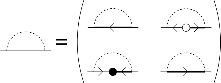
Abbildung 2.2: Diagrammatic representation of Eq. (2.21). The quark self-energy is shown as a $2\times 2$ Nambu-Gor’kov matrix (cf. also Eqs. (2.22)). Dashed lines correspond to the gluon propagator $\Delta$. The normal full quasiparticle propagators $G^{+}$ and $G^{-}$ are denoted by thick lines with an arrow pointing to the left and right, respectively. The anomalous propagators $\Xi^{\pm}$ are drawn according to their structure given in Eq. (2.20): Thin lines correspond to the term $([G_{0}^{\mp}]^{-1}+\Sigma^{\mp})^{-1}$, while the full and empty circles denote the gap matrices $\Phi^{+}$ and $\Phi^{-}$, respectively.

The last two equations, Eqs. (2.22c) and (2.22d), are the gap equations. The quantities $\Phi^{\pm}(K)$ are matrices in flavor, color, and Dirac space and functions of the quark four-momentum $K$. They occur on the left-hand side of the equations as well as on the right-hand side, implicitly present under the integral in the anomalous propagators. Both quantities are related via

$$\Phi^{-}=\gamma_{0}[\Phi^{+}]^{\dagger}\gamma_{0}\,\,.$$ (2.23)

In the following, we will use the term gap matrix for $\Phi^{+}(K)$. A complete self-consistent solution of the four coupled integral equations is too difficult and certain approximations have to be made. In Secs. 2.1.3 and 2.1.4, we use the gap equation to determine the value of the gap at the Fermi surface for $T=0$ and the critical temperature $T_{c}$. In the next section, Sec. 2.1.2, we determine the structure of the quasiparticle excitation energies which follows from the ansatz for the gap matrix $\Phi^{+}$ (without solving the gap equation).

2.1.2 Excitation energies

Before we solve the gap equation, let us first investigate the structure of the full quasiparticle propagator $G^{+}$. From this propagator we can read off the excitation energy of the quasiparticles. This energy spectrum has a nonzero gap in the case of a superconductor, as discussed in Sec. 1.2.1. In this section, it is shown how the ansatz for the gap matrix, and especially the form of the order parameter, determines the excitation spectrum. Here and in all following sections of this thesis, for the sake of simplicity, we consider ultrarelativistic quarks, $m=0$, which is a very good approximation at least for the $u$ and $d$ quarks. Nonzero quark masses cause tremendous technical complications [106]. In this case, restricting to Cooper pairing in the even-parity channel, the gap matrix can be written as

$$\Phi^{+}(K)=\sum_{e=\pm}\phi^{e}(K)\,{\cal M}_{\bf k}\,\Lambda^{e}_{\bf k}\,\,,$$ (2.24)

where $\phi^{e}(K)$ is the gap function, ${\cal M}_{\bf k}$ is a matrix defined by the symmetries of the color-superconducting condensate, and $\Lambda_{\bf k}^{e}=(1+e\gamma_{0}\mbox{\boldmath${\gamma}$}\cdot\hat{\mathbf{k}})/2$, $e=\pm$, are projectors onto states of positive or negative energy. In general, ${\cal M}_{\bf k}$ is a matrix in color, flavor, and Dirac space, and it can be chosen such that

$$[{\cal M}_{\bf k},\Lambda^{e}_{\bf k}]=0\,\,.$$ (2.25)

Let us comment on the relation between the matrix ${\cal M}_{\bf k}$ and the order parameter $\Delta$ discussed in the introduction of this thesis. In the matrix ${\cal M}_{\bf k}$ not only the order parameter $\Delta$ is implicitly present but also the basis elements of the special representation of the underlying symmetry groups accounting for the (anti-)symmetry of the representation. As explained in the introduction, the representation solely depends on the number of flavors, while the choice of the order parameter corresponds to a special phase. This will become more transparent below, in Sec. 2.1.2, when ${\cal M}_{\bf k}$ is specified for several numbers of flavors and several phases, see, for instance, Eq. (2.86). What might appear awkward at first sight, but is technically convenient, is that the $4\times 4$ Dirac structure is partially included into ${\cal M}_{\bf k}$ and partially explicitly written via the energy projectors. For details concerning the Dirac structure of the gap matrix, cf. Ref. [107].

Using Eq. (2.19), we can write the quasiparticle propagator as

$$G^{+} = ([G^{-}_{0}]^{-1}+\Sigma^{-})\left\{([G_{0}^{+}]^{-1}+\Sigma^{+})([G^{-}_{0}]^{-1}+\Sigma^{-})\right.$$ (2.26)

$$\left.-\;\Phi^{-}([G_{0}^{-}]^{-1}+\Sigma^{-})^{-1}\Phi^{+}([G_{0}^{-}]^{-1}+\Sigma^{-})\right\}^{-1}\,\,.$$

The free fermion (charge-conjugate) propagator for massless quarks in momentum space is

$$G_{0}^{\pm}(K)=(\gamma^{\mu}K_{\mu}\pm\mu\gamma_{0})^{-1}\,\,,$$ (2.27)

In Ref. [108], it was shown that, in order to solve the gap equation to subleading order, it is permissible to approximate the diagonal elements of the quark self-energy by

$$\Sigma(K)\equiv\Sigma^{+}(K)=\Sigma^{-}(K)\simeq\gamma_{0}\,\bar{g}^{2}\,k_{0}\,\ln\frac{M^{2}}{k_{0}^{2}}\,\,,$$ (2.28)

where

$$\bar{g}\equiv\frac{g}{3\sqrt{2}\pi}\,\,,\qquad M^{2}\equiv\frac{3\pi}{4}m_{g}^{2}\,\,,$$ (2.29)

and the zero-temperature gluon mass parameter (squared) is

$$m_{g}^{2}\equiv\frac{N_{f}g^{2}\mu^{2}}{6\pi^{2}}\,\,.$$ (2.30)

Then, using the above ansatz for the gap matrix, the second term in curly brackets in Eq. (2.26) is

$$\Phi^{-}([G_{0}^{-}]^{-1}+\Sigma^{-})^{-1}\Phi^{+}([G_{0}^{-}]^{-1}+\Sigma^{-})=\sum_{e}|\phi^{e}(K)|^{2}\,L_{\bf k}\,\Lambda^{-e}_{\bf k}\,\,,$$ (2.31)

where

$$L_{\bf k}\equiv\gamma_{0}\,{\cal M}^{\dagger}_{\bf k}{\cal M}_{\bf k}\,\gamma_{0}\,\,.$$ (2.32)

In principle, a notation that includes a “+”, such as $L^{+}_{\bf k}$, would be appropriate since, in general, the corresponding matrix $L^{-}_{\bf k}$ occurring in the expression for the charge-conjugate propagator $G^{-}$ might be different. Indeed, in one of the phases we consider in this thesis, namely the A phase in a spin-one color superconductor, we have $L^{+}_{\bf k}\neq L^{-}_{\bf k}$. For more details concerning this special case, see Sec. 2.4. Here and in the following sections it is sufficient to consider $L_{\bf k}\equiv L^{+}_{\bf k}$, since in the gap equation, only $G^{+}$ and not $G^{-}$ occurs, and thus we simplify the notation by omitting the +.

Note that also $L_{\bf k}$ commutes with the energy projectors, $[L_{\bf k},\Lambda_{\bf k}^{e}]=0$. Since $L_{\bf k}$ is hermitian, it has real eigenvalues and can be expanded in terms of a complete set of orthogonal projectors ${\cal P}_{\bf k}^{r}$,

$$L_{\bf k}=\sum_{r}\lambda_{r}\,{\cal P}_{\bf k}^{r}\,\,,$$ (2.33)

where $\lambda_{r}$ are the eigenvalues of $L_{\bf k}$. In this decomposition, the sum over $r$ is defined such that all $\lambda_{r}$ are different, i.e., the corresponding projectors ${\cal P}_{\bf k}^{r}$ project onto $n_{r}$-dimensional eigenspaces, where $n_{r}\equiv{\rm Tr}{\cal P}_{\bf k}^{r}$ is the degeneracy of the eigenvalue $\lambda_{r}$. In general, these eigenvalues can depend on the direction of the quark 3-momentum ${\bf k}$. For the sake of notational convenience, we do not write this $\hat{\mathbf{k}}$-dependence explicitly. Denoting the number of different eigenvalues with $n$, the projectors can be computed via

$${\cal P}_{\bf k}^{r}=\prod_{s\neq r}^{n}\frac{L_{\bf k}-\lambda_{s}}{\lambda_{r}-\lambda_{s}}\,\,.$$ (2.34)

For a proof of this relation, see Appendix A. Obviously, these projectors also commute with the energy projectors, $[{\cal P}_{\bf k}^{r},\Lambda_{\bf k}^{e}]=0$. The maximum number of different eigenvalues for the color-superconducting phases we consider in this thesis is $n=3$. However, we solve the gap equation only for special cases in which there are at most two different eigenvalues of $L_{\bf k}$. Therefore, let us explicitly write the expression for the projectors in this case,

$${\cal P}_{\bf k}^{1,2}=\frac{L_{\bf k}-\lambda_{2,1}}{\lambda_{1,2}-\lambda_{2,1}}\,\,.$$ (2.35)

The next step is to compute the full quasiparticle propagator $G^{+}$. The inversion of the term in curly brackets in Eq. (2.26) is now particularly simple, because the $2n$ projectors ${\cal P}_{\bf k}^{r}\Lambda_{\bf k}^{\pm}$ are orthogonal and form a complete set in color, flavor, and Dirac space. With Eqs. (2.26), (2.28), (2.31), and (2.33) we obtain

$$G^{+}(K)=([G_{0}^{-}(K)]^{-1}+\Sigma^{-}(K))\sum_{e,r}{\cal P}_{\bf k}^{r}\,\Lambda_{\bf k}^{-e}\,\frac{1}{\left[k_{0}/Z(k_{0})\right]^{2}-\left[\epsilon_{k,r}^{e}(\phi^{e})\right]^{2}}\,\,,$$ (2.36)

where

$$Z(k_{0})\equiv\left(1+\bar{g}^{2}\,\ln\frac{M^{2}}{k_{0}^{2}}\right)^{-1}$$ (2.37)

is the wave function renormalization factor introduced in Ref. [105], and

$$\epsilon_{k,r}^{e}(\phi^{e})\equiv\left[(k-e\mu)^{2}+\lambda_{r}|\phi^{e}|^{2}\right]^{1/2}$$ (2.38)

are the excitation energies for quasiparticles, $e=+$, or quasi-antiparticles, $e=-$. They are the relativistic analogues to Eq. (1.2), extended by a possibly nontrivial (multi-)gap structure, which also includes possible anisotropies of the “true” gaps $\sqrt{\lambda_{r}}\,|\phi^{e}|$. It was the goal of this section to show that the investigation of this gap structure is equivalent to studying the spectrum of the matrix $L_{\bf k}$.

2.1.3 Solution of the gap equation

In this section, we present a method to compute the value of the gap at the Fermi surface at zero temperature from the gap equation. In the case of the 2SC phase, this value is given by

$$\phi_{0}^{\rm 2SC}=2\,\tilde{b}\,b_{0}^{\prime}\,\mu\,\exp\left(-\frac{\pi}{2\,\bar{g}}\right)\,\,,$$ (2.39)

where

$$\tilde{b}\equiv 256\pi^{4}\left(\frac{2}{N_{f}g^{2}}\right)^{5/2}\,\,,\qquad b_{0}^{\prime}\equiv\exp\left(-\frac{\pi^{2}+4}{8}\right)\,\,.$$ (2.40)

The term in the exponent of Eq. (2.39) was first computed by Son [91]. It arises from the exchange of almost static magnetic gluons. The factor $\tilde{b}$ in front of the exponential originates from the exchange of static electric and non-static magnetic gluons [61, 92, 93]. The prefactor $b_{0}^{\prime}$ is due to the quark self-energy [108, 109].

In color superconductors with $N_{f}=1$ and 3 flavors, various other prefactors may arise [62, 110], but the exponential $\exp[-\pi/(2\bar{g})]$ remains the same. As will be demonstrated in the following, this is not an accident, but due to the fact that the leading-order contribution to the QCD gap equation does not depend on the detailed color, flavor, and Dirac structure of the color-superconducting order parameter. This structure only enters at subleading order, and we provide a simple method to extract these subleading contributions.

Let us briefly recall what the terms “leading,” “subleading,” and “sub-subleading order” mean in the context of the QCD gap equation [108]. Due to the non-analytic dependence of $\phi_{0}$ on the strong coupling constant $g$ one cannot apply the naive perturbative counting scheme in powers of $g$ in order to identify contributions of different order. In the QCD gap equation there are also logarithms of the form $\ln(\mu/\phi_{0})$, which are $\sim 1/g$ due to Eq. (2.39) and thus may cancel simple powers of $g$. A detailed discussion of the resulting, modified power-counting scheme was given in the introduction of Ref. [108] and need not be repeated here. In short, leading-order contributions in the QCD gap equation are due to the exchange of almost static magnetic gluons and are proportional to $g^{2}\,\phi_{0}\,\ln^{2}(\mu/\phi_{0})\sim\phi_{0}$. They determine the argument of the exponential in Eq. (2.39). Subleading-order contributions are due to the exchange of static electric and non-static magnetic gluons and are $\sim g^{2}\,\phi_{0}\,\ln(\mu/\phi_{0})\sim g\,\phi_{0}$. They determine the prefactor of the exponential in Eq. (2.39). Finally, sub-subleading contributions arise from a variety of sources and, at present, cannot be systematically calculated. They are proportional to $g^{2}\,\phi_{0}$ and constitute $O(g)$ corrections to the prefactor in Eq. (2.39). It was argued that also gauge-dependent terms enter at this order [111]. This is, of course, an artefact of the mean-field approximation which was used to derive the QCD gap equation [107]. On the quasiparticle mass shell, the true gap parameter is in principle a physical observable and thus cannot be gauge dependent.

Let us anticipate the most important results of this section. The general result for the gap parameter, which will be proven in the remainder of this section, is (if $L_{\bf k}$ has two different eigenvalues $\lambda_{1}$, $\lambda_{2}$)

$$\phi_{0}=2\,\,b\,b_{0}^{\prime}\,\mu\,\exp\left(-\frac{\pi}{2\,\bar{g}}\right)\,\left(\langle\lambda_{1}\rangle^{a_{1}}\,\langle\lambda_{2}\rangle^{a_{2}}\right)^{-1/2}\,\,,$$ (2.41)

where $a_{1},a_{2}$ are positive constants obeying the constraint

$$a_{1}+a_{2}=1\,\,.$$ (2.42)

With $\langle-\rangle$ we denote the angular average (in the case of the spin-one phases, the eigenvalues might depend on the direction of the quark momentum ${\bf k}$),

$$\langle\lambda_{r}\rangle\equiv\int\frac{d\Omega_{\bf k}}{4\pi}\lambda_{r}\,\,.$$ (2.43)

The constant $b$ is defined as

$$b\equiv\tilde{b}\,\exp(-d)\,\,,$$ (2.44)

with $\tilde{b}$ from Eq. (2.40), and $d$ a constant of order one. The constant $d$ originates from subleading contributions to the gap equation. For spin-zero condensates, $d=0$, due to an accidental cancellation of some of the subleading terms arising from static electric and non-static magnetic gluon exchange. In the spin-one cases, this cancellation does not occur and, consequently, $d\neq 0$. Actually, in one of the spin-one phases considered below, $d$ is not a constant but depends on the direction of the quark momentum, $d=d(\hat{\mathbf{k}})$. Nevertheless, let us keep the simplified notation $d$ without explicitly writing a potential $\hat{\mathbf{k}}$ dependence (as we also do for the eigenvalues $\lambda_{1}$, $\lambda_{2}$).

From Eqs. (2.39) and (2.41) one immediately determines $\phi_{0}$ in units of the gap in the 2SC phase,

$$\frac{\phi_{0}}{\phi_{0}^{\rm 2SC}}=\exp(-d)\,\left(\langle\lambda_{1}\rangle^{a_{1}}\,\langle\lambda_{2}\rangle^{a_{2}}\right)^{-1/2}\,\,.$$ (2.45)

In this thesis we present a simple method to extract the value of the constant $d$ without actually solving a gap equation. This method utilizes the fact that, to subleading order, the integration over gluon momenta in the QCD gap equation can be written as a sum of a few integrals multiplied by constants. Only these constants depend on the detailed color, flavor, and Dirac structure of the order parameter. The integrals are generic for all cases studied here and have to be computed only once.

This is a nontrivial fact. It means that the leading contribution to the gap equation is unique. If it were not, then the prefactor of the gap integral would be different for each case. In other words, the contribution of almost static magnetic gluons to the gap equation is universal in the sense that it is independent of the detailed color, flavor, and Dirac structure of the color-superconducting order parameter. Differences between the cases studied here occur at subleading order. Only at this order the specific structure of the order parameter is important and leads to different values for the constant $d$ in Eq. (2.44).

Let us now start to prove Eq. (2.41) (and consequently also Eq. (2.45)) using the gap equation, Eq. (2.22c). For the right-hand side of this equation we need the anomalous propagator $\Xi^{+}(K)$, defined in Eq. (2.20). Inserting the expression for the propagator $G^{+}$, Eq. (2.36), into this definition and using the form of the gap matrix $\Phi^{+}$ given in Eq. (2.24), we obtain

$$\Xi^{+}(K)=-\sum_{e,r}\gamma_{0}\,{\cal M}_{\bf k}\,\gamma_{0}\,{\cal P}_{\bf k}^{r}\Lambda_{\bf k}^{-e}\,\frac{\phi^{e}(K)}{\left[k_{0}/Z(k_{0})\right]^{2}-\left[\epsilon_{k,r}^{e}(\phi^{e})\right]^{2}}\,\,.$$ (2.46)

To derive the gap equation for the gap function $\phi^{e}(K)$, we insert Eq. (2.46) into Eq. (2.22c), multiply both sides from the right with ${\cal M}^{\dagger}_{\bf k}\,\Lambda_{\bf k}^{e}$ and trace over color, flavor, and Dirac space. To subleading order in the gap equation, it is permissible to use the gluon propagator in the Hard-Dense-Loop (HDL) approximation [112], where it is diagonal in adjoint color space, $\Delta^{\mu\nu}_{ab}=\delta_{ab}\,\Delta^{\mu\nu}$. We obtain

$$\phi^{e}(K)=g^{2}\frac{T}{V}\sum_{Q}\sum_{e^{\prime},s}\frac{\phi^{e^{\prime}}(Q)}{\left[q_{0}/Z(q_{0})\right]^{2}-\left[\epsilon_{q,s}^{e^{\prime}}(\phi^{e^{\prime}})\right]^{2}}\,\Delta^{\mu\nu}(K-Q)\,{\cal T}_{\mu\nu}^{ee^{\prime},s}({\bf k},{\bf q})\,\,,$$ (2.47)

where the sum over $s$ corresponds to the two eigenvalues $\lambda_{1}$ and $\lambda_{2}$, i.e., $s=1,2$, and

$${\cal T}_{\mu\nu}^{ee^{\prime},s}({\bf k},{\bf q})\equiv-\frac{{\rm Tr}\left[\gamma_{\mu}\,T_{a}^{T}\,\gamma_{0}\,{\cal M}_{\bf q}\,\gamma_{0}\,{\cal P}_{\bf q}^{s}\,\Lambda_{\bf q}^{-e^{\prime}}\,\gamma_{\nu}\,T_{a}\,{\cal M}^{\dagger}_{\bf k}\,\Lambda_{\bf k}^{e}\right]}{{\rm Tr}\left[{\cal M}_{\bf k}\,{\cal M}^{\dagger}_{\bf k}\,\Lambda_{\bf k}^{e}\right]}\,\,.$$ (2.48)

The form (2.47) of the gap equation holds for all cases considered in this thesis. What is different in each case is the structure of the term ${\cal T}_{\mu\nu}^{ee^{\prime},s}({\bf k},{\bf q})$. Our computation will be done in pure Coulomb gauge, where

$$\Delta^{00}(P)=\Delta_{\ell}(P)\,\,,\,\,\,\Delta^{0i}(P)=0\,\,,\,\,\,\Delta^{ij}(P)=(\delta^{ij}-\hat{p}^{i}\hat{p}^{j})\,\Delta_{t}(P)\,\,,$$ (2.49)

with the longitudinal and transverse propagators $\Delta_{\ell,t}$ and $P\equiv K-Q$. Consequently, we only need the 00-component, ${\cal T}_{00}^{ee^{\prime},s}({\bf k},{\bf q})$, and the transverse projection of the $ij$-components,

$${\cal T}_{t}^{ee^{\prime},s}({\bf k},{\bf q})\equiv-(\delta^{ij}-\hat{p}^{i}\hat{p}^{j})\,{\cal T}_{ij}^{ee^{\prime},s}({\bf k},{\bf q})\,\,,$$ (2.50)

of the tensor (2.48). (The extra minus sign is included for the sake of notational convenience.) It will turn out that in all cases studied here the quantities ${\cal T}_{00,t}^{ee^{\prime},s}({\bf k},{\bf q})$ are related in the following way:

$$\frac{{\cal T}_{00}^{ee^{\prime},2}({\bf k},{\bf q})}{{\cal T}_{00}^{ee^{\prime},1}({\bf k},{\bf q})}=\frac{{\cal T}_{t}^{ee^{\prime},2}({\bf k},{\bf q})}{{\cal T}_{t}^{ee^{\prime},1}({\bf k},{\bf q})}=\mbox{const.}\,\,.$$ (2.51)

The right-hand side of Eq. (2.48) depends on $k$, $q$, and $\hat{\mathbf{k}}\cdot\hat{\mathbf{q}}$. The latter can be replaced by the square of the gluon 3-momentum $p^{2}$ via $\hat{\mathbf{k}}\cdot\hat{\mathbf{q}}=(k^{2}+q^{2}-p^{2})/(2kq)$. Thus, the relevant components can be written in terms of a power series in $p^{2}$,

$${\cal T}_{00}^{ee^{\prime},s}({\bf k},{\bf q}) = a_{s}\sum_{m=-1}^{\infty}\,\eta_{2m}^{\ell}(ee^{\prime},k,q)\,\left(\frac{p^{2}}{kq}\right)^{m}\,\,,$$ (2.52a)

$${\cal T}_{t}^{ee^{\prime},s}({\bf k},{\bf q}) = a_{s}\sum_{m=-1}^{\infty}\,\eta_{2m}^{t}(ee^{\prime},k,q)\,\left(\frac{p^{2}}{kq}\right)^{m}\,\,.$$ (2.52b)

Here, the coefficients $\eta_{2m}^{\ell,t}(ee^{\prime},k,q)$ no longer depend on $s$ on account of Eq. (2.51). The overall normalization on the right-hand sides of Eqs. (2.52) is still free, and we choose it such that Eq. (2.42) is fulfilled. This uniquely determines the values of the dimensionless coefficients $\eta_{2m}^{\ell,t}(ee^{\prime},k,q)$ and we have the following relation for the coefficients $a_{1}$, $a_{2}$,

$$a_{1/2}\equiv\frac{{\cal T}_{t}^{ee^{\prime},1/2}({\bf k},{\bf q})}{{\cal T}_{t}^{ee^{\prime},1}({\bf k},{\bf q})+{\cal T}_{t}^{ee^{\prime},2}({\bf k},{\bf q})}=\frac{{\cal T}_{00}^{ee^{\prime},1/2}({\bf k},{\bf q})}{{\cal T}_{00}^{ee^{\prime},1}({\bf k},{\bf q})+{\cal T}_{00}^{ee^{\prime},2}({\bf k},{\bf q})}\,\,.$$ (2.53)

We now perform the Matsubara sum in Eq. (2.47), which does not depend on the detailed structure of the tensor ${\cal T}_{\mu\nu}^{ee^{\prime},s}({\bf k},{\bf q})$. This calculation is similar to that of Ref. [61]. The difference is the appearance of the wave function renormalization factor $Z(q_{0})$ [108]. To subleading order, this amounts to an extra factor $Z(\epsilon_{q,s}^{e^{\prime}})$ in the gap equation. Since there are two different excitation energies $\epsilon_{q,1}$ and $\epsilon_{q,2}$ on the right-hand side of the gap equation, we can put the gap function on the left-hand side on either one of the two possible quasiparticle mass shells $k_{0}=\epsilon_{k,1}$ or $k_{0}=\epsilon_{k,2}$. One then obtains

$$\phi^{e}(\epsilon_{k,r}^{e},k) = \frac{g^{2}}{16\pi^{2}k}\int_{\mu-\delta}^{\mu+\delta}dq\,q\sum_{e^{\prime},s}a_{s}\,Z(\epsilon_{q,s}^{e^{\prime}})\,\frac{\phi^{e^{\prime}}(\epsilon_{q,s}^{e^{\prime}},q)}{\epsilon_{q,s}^{e^{\prime}}}\,\tanh\left(\frac{\epsilon_{q,s}^{e^{\prime}}}{2T}\right)$$ (2.54)

$$\times\sum_{m}\int_{|k-q|}^{k+q}dp\,p\left(\frac{p^{2}}{kq}\right)^{m}\,\left\{\frac{2}{p^{2}+3m_{g}^{2}}\,\eta_{2m}^{\ell}+\left[\;\frac{2}{p^{2}}\,\Theta(p-M)\right.\right.$$

$$\left.\left.+\Theta(M-p)\left(\frac{p^{4}}{p^{6}+M^{4}(\epsilon_{q,s}^{e^{\prime}}+\epsilon_{k,r}^{e})^{2}}+\frac{p^{4}}{p^{6}+M^{4}(\epsilon_{q,s}^{e^{\prime}}-\epsilon_{k,r}^{e})^{2}}\right)\right]\eta_{2m}^{t}\right\}\,\,.$$

The first term in braces arises from static electric gluons, while the two terms in brackets originate from non-static and almost static magnetic gluons, respectively. Various other terms which yield sub-subleading contributions to the gap equation [61] have been omitted. In deriving Eq. (2.54), the angular integration $d\Omega_{\bf q}=\sin\theta d\theta d\varphi$ has been reduced to an integration over the modulus of the gluon momentum $p$: The integral over the polar angle $\theta$ can be transformed into an integral over $p$ by choosing the coordinate system such that $\hat{\mathbf{k}}\cdot\hat{\mathbf{q}}=\cos\theta$ and applying the relation $\hat{\mathbf{k}}\cdot\hat{\mathbf{q}}=(k^{2}+q^{2}-p^{2})/(2kq)$. The integration over the azimuthal angle $\varphi$ has already been performed. This integration is trivial in the 2SC and CFL phases, since in these cases the gap function only depends on the modulus of ${\bf q}$ and the eigenvalues $\lambda_{s}$ are constants. However, in the spin-one phases, there might occur angular dependent terms, and consequently, the $d\Omega_{\bf q}$ integration becomes nontrivial. First, through a potential angular dependence of $\lambda_{s}$, the excitation energies in the integrand can be $\hat{\mathbf{q}}$-dependent. Second, the gap function itself may turn out to depend on $\hat{\mathbf{q}}$. In order to proceed, we approximate the angular integral by replacing the eigenvalues in the excitation energies $\epsilon_{q,s}^{e^{\prime}}$ by their angular averages

$$\lambda_{s}\to\langle\lambda_{s}\rangle\,\,,$$ (2.55)

and then performing the resulting integral over the azimuthal angle and over $p$. In order to avoid a too complicated notation, we keep the same symbols for the excitation energies, $\epsilon_{q,s}^{e^{\prime}}$, but understand them with the above replacement. This simple approximation is based on the assumption that all neglected terms are of sub-subleading order, for which, in principle, a rigorous proof is required. An angular-dependent gap function $\phi^{e^{\prime}}(\epsilon_{q,s}^{e^{\prime}},q)$ occurs in one of the spin-one phases, namely the polar phase. This dependence, entering via an angular dependent function $d=d(\hat{\mathbf{q}})$, is neglected here, cf. also comments in the discussion of this phase, Sec. 2.1.5.

Although the coefficients $\eta_{2m}^{\ell,t}$ depend on $k$ and $q$, to subleading order in the gap equation we may approximate $k\simeq q\simeq\mu$. This can be easily proven by power counting. To this end, it is sufficient to take $k=\mu$, and write $q=\mu+\xi$, where $\xi=q-\mu$. In weak coupling, the gap function is sharply peaked around the Fermi surface, and thus the range of integration in the gap equation can be restricted to a small region of size $2\,\delta$ around the Fermi surface. All that is necessary is that $\delta$ is parametrically much larger than $\phi_{0}$, but still much smaller than $\mu$, $\phi_{0}\ll\delta\ll\mu$ [61]. It turns out that $\delta\sim m_{g}$ is a convenient choice [113]. Since the integral over $\xi$ is symmetric around $\xi=0$, terms proportional to odd powers of $\xi$ vanish by symmetry. Thus, corrections to the leading-order terms are at most $\sim(\xi/\mu)^{2}$. As long as $\delta$ is parametrically of the order of $m_{g}$, $\xi\leq m_{g}$, and these corrections are $\sim g^{2}$, i.e., suppressed by two powers of the coupling constant. Even for the leading terms in the gap equation the correction due to terms $\sim(\xi/\mu)^{2}$ is then only of sub-subleading order and thus negligible.

Since the coefficients $\eta_{2m}^{\ell,t}$ are dimensionless, with the approximation $k\simeq q\simeq\mu$ they become pure numbers which, as we shall see in the following, are directly related to the constant $d$. In all cases considered here, $\eta_{2m}^{\ell,t}=0$ for $m\geq 3$, and the series in Eqs. (2.52) terminate after the first few terms. Moreover, $\eta_{-2}^{\ell}$ always vanishes and, to subleading order, also $\eta_{-2}^{t}=0$. For the remaining $m$, the $p$ integral in Eq. (2.54) can be performed exactly. The details of this calculation are deferred to Appendix B. We obtain

$$\phi^{e}(\epsilon_{k,r}^{e},k) = \frac{g^{2}}{16\pi^{2}}\int_{\mu-\delta}^{\mu+\delta}dq\sum_{e^{\prime},s}a_{s}\,Z(\epsilon_{q,s}^{e^{\prime}})\,\frac{\phi^{e^{\prime}}(\epsilon_{q,s}^{e^{\prime}},q)}{\epsilon_{q,s}^{e^{\prime}}}\,\tanh\left(\frac{\epsilon_{q,s}^{e^{\prime}}}{2T}\right)$$ (2.56)

$$\times\left[\eta_{0}^{t}\,\frac{1}{3}\,\ln\frac{M^{2}}{|(\epsilon_{q,s}^{e^{\prime}})^{2}-(\epsilon_{k,r}^{e})^{2}|}+\eta_{0}^{\ell}\,\ln\frac{4\mu^{2}}{3m_{g}^{2}}\right.$$

$$\left.+\eta_{0}^{t}\,\ln\frac{4\mu^{2}}{M^{2}}+4(\eta_{2}^{\ell}+\eta_{2}^{t})+8(\eta_{4}^{\ell}+\eta_{4}^{t})\right]\;.$$

Note that the contribution from almost static magnetic gluons only appears in the term proportional to $\eta_{0}^{t}$, while non-static magnetic and static electric gluons contribute to all other terms.

The antiparticle contribution ($e^{\prime}=-$) does not have a BCS logarithm, since $\epsilon_{q,s}^{-}\simeq q+\mu$. For the same reason, for antiparticles the logarithm from almost static magnetic gluons is also only of order 1, and furthermore there is no large logarithm from the $p$ integrals. Therefore, the antiparticles contribute at most to sub-subleading order to the gap equation and can be neglected. In the following, we may thus set $e=e^{\prime}=+$ and omit this superscript for the sake of simplicity. Then, the gap equation for the quasiparticle gap function reads

$$\phi(\epsilon_{k,r},k)=\bar{g}^{2}\int_{0}^{\delta}d(q-\mu)\;\sum_{s}a_{s}\,Z(\epsilon_{q,s})\,\frac{\phi(\epsilon_{q,s},q)}{\epsilon_{q,s}}\;\tanh\left(\frac{\epsilon_{q,s}}{2T}\right)\;\frac{3}{4}\,\eta_{0}^{t}\,\ln\left(\frac{b^{2}\mu^{2}}{|\epsilon_{q,s}^{2}-\epsilon_{k,r}^{2}|}\right)\,\,,$$ (2.57)

where

$$b^{2}=\frac{64\,\mu^{4}}{M^{4}}\left(\frac{4\mu^{2}}{3m_{g}^{2}}\right)^{3\eta_{0}^{\ell}/\eta_{0}^{t}}\exp(-2d)\,\,,$$ (2.58)

with

$$d=-\frac{6}{\eta_{0}^{t}}\,\left[\eta_{2}^{\ell}+\eta_{2}^{t}+2(\eta_{4}^{\ell}+\eta_{4}^{t})\right]\,\,.$$ (2.59)

In all cases considered here, $\eta_{0}^{\ell}=\eta_{0}^{t}$, so that $b$ assumes the value quoted in Eq. (2.44). The expression (2.59) is a general formula to compute the constant $d$ from the coefficients $\eta_{2m}^{\ell,t}$. We also find that, for all cases considered here, $\eta_{0}^{t}=2/3$. This is the uniqueness of the leading-order contribution to the gap equation mentioned before.

Let us, in order to solve Eq. (2.57), distinguish between the cases where $a_{1}=1,\,a_{2}=0$, and where both $a_{1}$ and $a_{2}$ are nonzero. It turns out that the former case corresponds to only one gapped quasiparticle excitation, i.e., $\lambda_{2}=0$. This is expected, since in this case, due to $a_{2}=0$, the ungapped excitation is not present in the gap equation. The solution of the gap equation is well-known for this case. It was discussed in detail in Ref. [108]. All one has to do is replace the constant $\tilde{b}$ in the calculation of Ref. [108] by the constant $b=\tilde{b}\exp(-d)$, cf. Eq. (2.44). The result for the value of the gap function at the Fermi surface is Eq. (2.41), but without the factor $(\langle\lambda_{1}\rangle^{a_{1}}\,\langle\lambda_{2}\rangle^{a_{2}})^{-1/2}$. However, in the respective cases this factor simply is $\langle\lambda_{1}\rangle^{-1/2}$ (remember that $0^{0}=1$). This factor is easily reproduced using the method presented in Ref. [108]: One has to multiply both sides of Eq. (2.57) with $\langle\lambda_{1}\rangle^{1/2}$ in order to obtain a gap equation for which the solution of Ref. [108] applies.

In the case of two gapped quasiparticle excitations, which is equivalent to $a_{1}\neq 0$, $a_{2}\neq 0$, the solution of Eq. (2.57) is more complicated. A priori, one has to solve two gap equations, one for each quasiparticle mass shell, $k_{0}=\epsilon_{k,1}$ and $k_{0}=\epsilon_{k,2}$. Therefore, as a function of momentum $k$, there are in principle two different gap functions, $\phi_{r}(k)\equiv\phi(\epsilon_{k,r},k),\,r=1,2$.

In order to proceed with the solution, to subleading order we may approximate the logarithm in Eq. (2.57) in a way first proposed by Son [91],

$$\frac{1}{2}\,\ln\left(\frac{b^{2}\mu^{2}}{|\epsilon_{q,s}^{2}-\epsilon_{k,r}^{2}|}\right)\simeq\Theta(\epsilon_{q,s}-\epsilon_{k,r})\,\ln\left(\frac{b\mu}{\epsilon_{q,s}}\right)+\Theta(\epsilon_{k,r}-\epsilon_{q,s})\,\ln\left(\frac{b\mu}{\epsilon_{k,r}}\right)\,\,.$$ (2.60)

With this approximation and the new variables

$$x_{r}\equiv\bar{g}\,\ln\left(\frac{2b\mu}{k-\mu+\epsilon_{k,r}}\right)\quad,\qquad y_{s}\equiv\bar{g}\,\ln\left(\frac{2b\mu}{q-\mu+\epsilon_{q,s}}\right)\,\,,$$ (2.61)

to subleading order the gap equation (2.57) transforms into [108]

$$\phi(x_{r}) = \sum_{s}a_{s}\left\{x_{r}\int_{x_{r}}^{x_{s}^{*}}dy_{s}\,(1-2\,\bar{g}\,y_{s})\,\tanh\left[\frac{\epsilon(y_{s})}{2T}\right]\,\phi(y_{s})\right.$$ (2.62)

$$\left.\hskip 28.45274pt+\int_{x_{0}}^{x_{r}}dy_{s}\,y_{s}\,(1-2\,\bar{g}\,y_{s})\,\tanh\left[\frac{\epsilon(y_{s})}{2T}\right]\,\phi(y_{s})\right\}\,\,.$$

Here, we denoted the value of $x_{s}$ at the Fermi surface, i.e, for $k=\mu$ and $\epsilon_{k,s}=\epsilon_{\mu,s}$, by

$$x_{s}^{*}\equiv\bar{g}\,\ln\left(\frac{2b\mu}{\sqrt{\langle\lambda_{s}\rangle}\,\phi_{0,s}}\right)\,\,,$$ (2.63)

where $\phi_{0,s}\equiv\phi(x_{s}^{*})$ is the value of the function $\phi(x_{s})$ at the Fermi surface. Remember that in the excitation energies $\epsilon_{q,s}$ we replaced $\lambda_{s}$ by the angular average $\langle\lambda_{s}\rangle$. The single point $k=\mu$ in momentum space thus corresponds to two different points $x_{1}^{*},\,x_{2}^{*}$, $x_{1}^{*}\neq x_{2}^{*}$ , in the new variables $x_{s}$. Since we expect $\phi_{0,s}$ to be $\sim\exp(-1/\bar{g})$, $x_{s}^{*}$ is a constant of order one. Furthermore we defined

$$x_{0}\equiv\bar{g}\,\ln\left(\frac{b\mu}{\delta}\right)\,\,.$$ (2.64)

This constant is parametrically of order $O(\bar{g})$. To subleading order, the relation between the new variable $y_{s}$ and the excitation energy is given by [61],

$$\epsilon(y_{s})=b\,\mu\,\exp\left(-\frac{y_{s}}{\bar{g}}\right)\,\,.$$ (2.65)

A consequence of the transformation of variables (2.61) and of neglecting sub-subleading corrections is that the two equations (2.62) for $r=1$ and $r=2$ become identical. The only difference is the notation for the argument of the function $\phi$, which in both cases we may simply call $x$. Therefore, instead of two separate equations, we only have to consider a single equation which determines the function $\phi(x)$. Moreover, $y_{s}$ is merely an integration variable, and we may set $y_{s}\equiv y$ in the following.

With Eq. (2.42), we rewrite Eq. (2.62) in the form

$$\phi(x) = x\int_{x}^{x_{2}^{*}}dy\,(1-2\,\bar{g}\,y)\,\tanh\left[\frac{\epsilon(y)}{2T}\right]\,\phi(y)+\int_{x_{0}}^{x}dy\,y\,(1-2\,\bar{g}\,y)\,\tanh\left[\frac{\epsilon(y)}{2T}\right]\,\phi(y)$$ (2.66)

$$-a_{1}\,x\int_{x_{1}^{*}}^{x_{2}^{*}}dy\,(1-2\,\bar{g}\,y)\,\tanh\left[\frac{\epsilon(y)}{2T}\right]\,\phi(y)\,\,.$$

One can also write this equation in a form where $x_{2}^{*}$ is replaced by $x_{1}^{*}$ and $a_{1}$ by $a_{2}$, respectively. Equation (2.66) is an integral equation for the function $\phi(x)$, which is solved in the standard manner by converting it into a set of differential equations [91],

$$\frac{d\phi}{dx} = \int_{x}^{x_{2}^{*}}dy\,(1-2\,\bar{g}\,y)\,\tanh\left[\frac{\epsilon(y)}{2T}\right]\,\phi(y)-a_{1}\int_{x_{1}^{*}}^{x_{2}^{*}}dy\,(1-2\,\bar{g}\,y)\,\tanh\left[\frac{\epsilon(y)}{2T}\right]\,\phi(y)\,\,,$$ (2.67a)

$$\frac{d^{2}\phi}{dx^{2}} = -(1-2\,\bar{g}\,x)\,\tanh\left[\frac{\epsilon(x)}{2T}\right]\,\phi(x)\,\,.$$ (2.67b)

We now solve the second-order differential equation (2.67b) at zero temperature, $T=0$. One immediately observes that this equation is identical to Eq. (22c) of Ref. [108], and its solution proceeds along the same lines as outlined there. The only difference compared to the previous calculation are the extra terms $\sim a_{1}$ in Eqs. (2.66) and (2.67a). To subleading order, we expect $\phi_{0,1}/\phi_{0,2}\simeq 1$ (we show below that this assumption is consistent with our final result), such that the difference

$$x_{2}^{*}-x_{1}^{*}=\bar{g}\,\ln\left(\frac{\sqrt{\langle\lambda_{1}\rangle}\,\phi_{0,1}}{\sqrt{\langle\lambda_{2}\rangle}\,\phi_{0,2}}\right)\simeq\frac{\bar{g}}{2}\,\ln\left(\frac{\langle\lambda_{1}\rangle}{\langle\lambda_{2}\rangle}\right)$$ (2.68)

is of order $O(\bar{g})$. Consequently, the extra terms $\sim a_{1}$ are of subleading order, $O(\bar{g}\phi_{0})$, and we may approximate

$$\int_{x_{1}^{*}}^{x_{2}^{*}}dy\,(1-2\,\bar{g}\,y)\,\,\phi(y)\simeq(x_{2}^{*}-x_{1}^{*})\,\phi_{0,2}\,\,.$$ (2.69)

Ordering the eigenvalues such that $\langle\lambda_{1}\rangle>\langle\lambda_{2}\rangle$, we have $x_{2}^{*}-x_{1}^{*}>0$.

The subleading correction (2.69) qualitatively changes the behavior of the gap function $\phi(x)$ near the Fermi surface. In the absence of the term $\sim a_{1}$ in Eq. (2.67a), the derivative of the gap function vanishes for $x=x_{2}^{*}$, and the gap function assumes its maximum at this point [108]. The subleading correction (2.69) induced by the two-gap structure causes the derivative (2.67a) of the function $\phi(x)$ to be negative at the Fermi surface. Consequently, since we still expect $\phi(x)$ to rapidly vanish away from the Fermi surface, this function assumes its maximum not right at the Fermi surface, but at a point $x_{\rm max}$ which is close, but not identical to $x_{2}^{*}$. We shall see that $x_{2}^{*}-x_{\rm max}\sim O(\bar{g})$.

The subleading correction (2.69) modifies the solution of the differential equation (2.67b) from the one given in Ref. [108]. Again, we fix the two unknown constants in the general solution of the second-order differential equation (2.67b) by matching the solution and its derivative to the right-hand sides of Eqs. (2.66) and (2.67a) at the point $x=x_{2}^{*}$. Introducing the variables $z\equiv-(2\bar{g})^{-2/3}\,(1-2\bar{g}x)$ and $z^{*}\equiv-(2\bar{g})^{-2/3}\,(1-2\bar{g}x_{2}^{*})$, the solution reads

$$\phi(z) = \phi_{0,2}\left\{\frac{M(|z|)}{M(|{z^{*}}|)}\frac{\sin\left[\varphi(|z^{*}|)-\theta(|z|)\right]}{\sin\left[\varphi(|z^{*}|)-\theta(|z^{*}|)\right]}\right.$$ (2.70)

$$\left.+a_{1}\,(x_{2}^{*}-x_{1}^{*})\,(2\bar{g})^{-1/3}\,\frac{M(|z|)}{N(|{z^{*}}|)}\,\frac{\sin\left[\theta(|z^{*}|)-\theta(|z|)\right]}{\sin\left[\varphi(|z^{*}|)-\theta(|z^{*}|)\right]}\right\}\,\,,$$

where the functions $M(|z|),\,N(|z|),\,\varphi(|z|),$ and $\theta(|z|)$ are related to the Airy functions ${\rm Ai}(z),\,{\rm Bi}(z)$ and their derivatives in the standard way [114]. The derivative $d\phi(z)/dz$ can be obtained from Eq. (2.70) simply by replacing $M(|z|)$ and $\theta(|z|)$ by $N(|z|)$ and $\varphi(|z|)$, respectively. The difference to the solution for a single gapped quasiparticle excitation, cf. Eq. (27) of Ref. [108], is the term proportional to $a_{1}$.

Finally, we have to determine the value of $\phi_{0,2}$. To this end, we rewrite Eq. (2.66) at the point $x=x_{2}^{*}$ in the form

$$\left[z_{0}+(2\bar{g})^{-2/3}\right]\,\frac{d\phi}{dz}(z_{0})=\phi(z_{0})\,\,,$$ (2.71)

where $z_{0}\equiv-(2\bar{g})^{-2/3}\,(1-2\bar{g}x_{0})$. Remarkably, this equation holds in this form also in the case of a single gapped quasiparticle excitation, cf. Eq. (29) of Ref.  [108]. In weak coupling, the dependence on the variable $z_{0}$ is spurious. Inserting the solution (2.70) and its derivative for $z=z_{0}$ and expanding $M(|z_{0}|),\,N(|z_{0}|),\,\varphi(|z_{0}|),$ and $\theta(|z_{0}|)$ to order $O(\bar{g})$ as demonstrated in Ref. [108], one derives the condition

$$x_{2}^{*}\simeq\frac{\pi}{2}+\bar{g}\,\frac{\pi^{2}+4}{8}+a_{1}\,(x_{2}^{*}-x_{1}^{*})\,\,.$$ (2.72)

The second term is the $O(\bar{g})$ correction originating from the quark self-energy. It leads to the constant $b_{0}^{\prime}$ in Eq. (2.39) and was first derived in Refs. [108, 109]. The last term $\sim a_{1}$ is the correction arising from the two-gap structure to the result (33) of Ref. [108]. Because of Eq. (2.68), this correction is also of order $O(\bar{g})$. Using the definition (2.63) of $x_{2}^{*}$, as well as the condition (2.42), we conclude that the expression for $\phi_{0,2}$ is identical to the one for $\phi_{0}$ in Eq. (2.41). This is the value of the gap function at the Fermi surface, $k=\mu$, or $x=x_{2}^{*}$, for the quasiparticle excitation branch $\epsilon_{k,2}$. The additional factor compared to the 2SC gap $\phi_{0}^{\rm 2SC}$ of Eq. (2.39), which originates from the two-gap structure, is $\left(\langle\lambda_{1}\rangle^{a_{1}}\,\langle\lambda_{2}\rangle^{a_{2}}\right)^{-1/2}$.

We can also compute the gap function at the Fermi surface for the first excitation branch $\epsilon_{k,1}$, i.e., at $x=x_{1}^{*}$. The difference $\phi_{0,2}-\phi_{0,1}$ can be obtained from Eq. (2.66) as

$$\phi_{0,2}-\phi_{0,1}=\int_{x_{1}^{*}}^{x_{2}^{*}}dy\,\left[y-x_{1}^{*}-a_{1}\,(x_{2}^{*}-x_{1}^{*})\right]\,(1-2\,\bar{g}\,y)\,\phi(y)\,\,.$$ (2.73)

An upper bound for the term in brackets is given by setting $y=x_{2}^{*}$, where it assumes the value $a_{2}(x_{2}^{*}-x_{1}^{*})$ on account of Eq. (2.42). Pulling this factor out of the integral, the latter can be estimated with Eq. (2.69). This proves that the difference $\phi_{0,2}-\phi_{0,1}$ is only of order $O(\bar{g}^{2}\phi_{0})$, which shows that our above assumption $\phi_{0,1}/\phi_{0,2}\simeq 1$ is consistent up to subleading order. To this order, we may therefore set $\phi_{0,1}=\phi_{0,2}\equiv\phi_{0}$.

We now determine the value of $x_{\rm max}$, where the gap function assumes its maximum, by setting the left-hand side of Eq. (2.67a) equal to zero. This leads to the condition

$$\int_{x_{\rm max}}^{x_{2}^{*}}dy\,(1-2\,\bar{g}\,y)\,\phi(y)=a_{1}\int_{x_{1}^{*}}^{x_{2}^{*}}dy\,(1-2\,\bar{g}\,y)\,\phi(y)\,\,.$$ (2.74)

To order $O(\bar{g}\phi_{0})$, one may easily solve this equation for $x_{\rm max}$, with the result

$$x_{\rm max}=x_{2}^{*}-a_{1}\,\frac{\bar{g}}{2}\,\ln\left(\frac{\langle\lambda_{1}\rangle}{\langle\lambda_{2}\rangle}\right)\,\,,$$ (2.75)

i.e., $x_{\rm max}$ is indeed smaller than $x_{2}^{*}$ by a term of order $O(\bar{g})$, as claimed above. Obviously, since $a_{1}<1$, from Eq. (2.68) we derive the inequality $x_{1}^{*}<x_{\rm max}<x_{2}^{*}$, i.e., the gap function assumes its maximum between the values $x_{1}^{*}$ and $x_{2}^{*}$. The value of the gap function at $x_{\rm max}$ can be estimated via a calculation similar to the one for the difference $\phi_{0,2}-\phi_{0,1}$ above. The result is $\phi_{max}\simeq\phi_{0}\,[1+O(\bar{g}^{2})]$. This means that the gap function is fairly flat over a region of size $O(\bar{g})$ (in the variable $x$) in the vicinity of the Fermi surface.

2.1.4 The critical temperature

In this section, we compute the critical temperature $T_{c}$ for the color-superconducting phase transition. Again, let us present the final result before we prove it. We find for the ratio of the critical temperature and the gap parameter

$$\frac{T_{c}}{\phi_{0}}=\frac{e^{\gamma}}{\pi}\,\left(\langle\lambda_{1}\rangle^{a_{1}}\,\langle\lambda_{2}\rangle^{a_{2}}\right)^{1/2}\simeq 0.57\,\left(\langle\lambda_{1}\rangle^{a_{1}}\,\langle\lambda_{2}\rangle^{a_{2}}\right)^{1/2}\,\,,$$ (2.76)

where $\gamma\simeq 0.577$ is the Euler-Mascheroni constant, already introduced in Eq. (1.5). In the case of $(\langle\lambda_{1}\rangle^{a_{1}}\,\langle\lambda_{2}\rangle^{a_{2}})^{1/2}=1$, we recover the relation (1.5) from BCS theory.

Note that, although a factor $(\langle\lambda_{1}\rangle^{a_{1}}\,\langle\lambda_{2}\rangle^{a_{2}})^{1/2}\neq 1$ renders the ratio $T_{c}/\phi_{0}$ different from BCS theory, the absolute value of $T_{c}$ is not affected by this factor. If the energy scale is set by $\phi_{0}^{\rm 2SC}$, then

$$\frac{T_{c}}{\phi_{0}^{\rm 2SC}}=\exp(-d)$$ (2.77)

because the factor $(\langle\lambda_{1}\rangle^{a_{1}}\,\langle\lambda_{2}\rangle^{a_{2}})^{-1/2}$ in Eq. (2.45) simply cancels the factor $(\langle\lambda_{1}\rangle^{a_{1}}\,\langle\lambda_{2}\rangle^{a_{2}})^{1/2}$ in Eq. (2.76). As mentioned above, in one of the cases we study, namely the polar phase, the gap function $\phi_{0}$ depends on the direction of the quark momentum. This dependence enters via the function $d=d({\bf k})$, cf. Sec. 2.1.5. In this case, Eq. (2.77) has to be replaced by

$$\frac{T_{c}}{\phi_{0}^{\rm 2SC}}=\langle\exp(-d)\rangle\,\,.$$ (2.78)

Let us now prove Eq. (2.76). In the case where $a_{1}=1$ and $a_{2}=0$, the calculation of Ref. [108] applies. Therefore, let us focus on the more complicated case where both $a_{1}$ and $a_{2}$ are nonzero. The calculation follows the line of arguments presented in Ref. [108], taking into account the additional term $\sim a_{1}$ in Eq. (2.66). As in Refs. [61, 108] we assume that, to leading order, the effect of temperature is a change of the magnitude of the gap, but not of the shape of the gap function,

$$\phi(x,T)\simeq\phi(T)\,\frac{\phi(x,0)}{\phi_{0}}\;,$$ (2.79)

where $\phi(T)\equiv\phi(x_{2}^{*},T)$ is the value of the gap at the Fermi surface at temperature $T$, $\phi(x,0)$ is the zero-temperature gap function $\phi(x)$ computed in the last section, cf. Eq. (2.70), and $\phi_{0}\equiv\phi_{0,2}=\phi(x_{2}^{*},0)$. With this assumption, Eq. (2.66) reads at the Fermi surface

$$1 = \int_{x_{0}}^{x_{\kappa}}dy\,y\,(1-2\,\bar{g}\,y)\,\tanh\left[\frac{\epsilon(y)}{2T}\right]\,\frac{\phi(y,0)}{\phi_{0}}+\int_{x_{\kappa}}^{x_{2}^{*}}dy\,y\,(1-2\,\bar{g}\,y)\,\tanh\left[\frac{\epsilon(y)}{2T}\right]\,\frac{\phi(y,0)}{\phi_{0}}$$ (2.80)

$$-a_{1}\,x_{2}^{*}\int_{x_{1}^{*}}^{x_{2}^{*}}dy\,(1-2\,\bar{g}\,y)\,\tanh\left[\frac{\epsilon(y)}{2T}\right]\,\frac{\phi(y,0)}{\phi_{0}}$$

$$\equiv {\cal I}_{1}+{\cal I}_{2}+{\cal I}_{3}\,\,,$$

where we divided the second integral in Eq. (2.66) into two integrals: ${\cal I}_{1}$ which runs from $x_{0}$ to $x_{\kappa}$, with $x_{\kappa}\equiv x_{2}^{*}-\bar{g}\,\ln(2\kappa)$, $\kappa\gg 1$, and ${\cal I}_{2}$ which runs from $x_{\kappa}$ to $x_{2}^{*}$ [61]. We now compute the integrals ${\cal I}_{1}$ through ${\cal I}_{3}$ separately to subleading accuracy, i.e., to order $O(\bar{g})$.

In the first integral ${\cal I}_{1}$, which runs over a region far from the Fermi surface, $\epsilon(y)\gg T$, and we may approximate the $\tanh$ by 1. This integral can be formally solved by integration by parts using the differential equation (2.67b),

$${\cal I}_{1}=\frac{1}{\phi_{0}}\,\left[\phi(x_{\kappa},0)-x_{\kappa}\,\frac{d\phi}{dx}(x_{\kappa},0)\right]\,\,,$$ (2.81)

where we exploited the condition (2.71). Expanding the functions on the right-hand side around $x_{2}^{*}$ we obtain to subleading order

$${\cal I}_{1}=1-\frac{\pi}{2}\,\left[\bar{g}\,\ln(2\kappa)-a_{1}\,(x_{2}^{*}-x_{1}^{*})\right]\,\,.$$ (2.82)

This estimate is similar to the one made in Eq. (36) of Ref. [108]. The main difference to that calculation is the term $\sim a_{1}$ which appears because the first derivative of the gap function no longer vanishes at the Fermi surface, cf. the discussion in the previous section.

In the second integral ${\cal I}_{2}$, which only contributes to order $O(\bar{g})$ to the right-hand side of Eq. (2.80), to subleading order we may set $\phi(y,0)/\phi_{0}\simeq 1$ and $y\simeq x_{2}^{*}\simeq\pi/2$. Reverting the transformation of variables (2.61) we obtain

$${\cal I}_{2}=\frac{\pi}{2}\bar{g}\int_{0}^{\sqrt{\langle\lambda_{2}\rangle}\kappa\phi_{0}}\frac{d(q-\mu)}{\epsilon_{q,2}}\,\tanh\left(\frac{\epsilon_{q,2}}{2T}\right)\,\,.$$ (2.83)

The last integral in Eq. (2.80), ${\cal I}_{3}$, also contributes a term of order $O(\bar{g})$, and may thus be approximated by an argument similar to that leading to Eq. (2.69),

$${\cal I}_{3}=a_{1}\,x_{2}^{*}(x_{2}^{*}-x_{1}^{*})\,\tanh\left[\frac{\phi(T)}{2T}\right]\,\,.$$ (2.84)

At the critical temperature $T_{c}$, where $\phi(T_{c})=0$, this term vanishes. Putting everything together, at $T=T_{c}$ Eq. (2.80) becomes

$$\bar{g}\int_{0}^{\sqrt{\langle\lambda_{2}\rangle}\kappa\phi_{0}}d(q-\mu)\,\left[\frac{1}{q-\mu}\,\tanh\left(\frac{q-\mu}{2T_{c}}\right)-\frac{1}{\sqrt{(q-\mu)^{2}+\langle\lambda_{2}\rangle\phi_{0}^{2}}}\right]=-a_{1}\,(x_{2}^{*}-x_{1}^{*})\,\,,$$ (2.85)

where the term $\ln(2\kappa)$ in Eq. (2.82) was expressed in terms of an integral according to Eq. (96) of Ref. [61]. In the integral on the left-hand side, we may send $\kappa\rightarrow\infty$ [61]. This allows us to perform it analytically, which yields the result $\ln[e^{\gamma}\sqrt{\langle\lambda_{2}\rangle}\phi_{0}/(\pi T_{c})]$. If the right-hand side of Eq. (2.85) were zero, for $\langle\lambda_{2}\rangle=1$ this would then lead to the BCS relation $T_{c}/\phi_{0}=e^{\gamma}/\pi$. However, using Eq. (2.68) we now obtain Eq. (2.76). The last factor on the right-hand side of this equation is exactly the inverse of the additional factor in Eq. (2.41). This factor violates the BCS relation $T_{c}/\phi_{0}=e^{\gamma}/\pi$.

2.1.5 Results: The 2SC, CFL, polar, planar, A, and CSL phases

In the previous sections we derived general expressions for the gap parameter and the critical temperature. The final expressions are given in Eqs. (2.41) and (2.76), respectively. In this section, we apply these expressions to spin-zero color superconductors in the 2SC and CFL phases, as well as to spin-one color superconductors in four different phases. For each case, we need to determine the following quantities:

• The eigenvalues $\lambda_{s}$ (and their degeneracies) of the matrix $L_{\bf k}$. This leads to the excitation spectrum, cf. Eq. (2.38).

• The projectors ${\cal P}_{\bf k}^{s}$, which project onto the corresponding eigenspaces. They are needed for

• the traces ${\cal T}_{00,t}^{ee^{\prime},s}({\bf k},{\bf q})$, defined in Eq. (2.48) and occurring in the gap equation.

• The constants $a_{1}$, $a_{2}$, introduced in Eqs. (2.52) and computed via Eq. (2.53).

• The coefficients $\eta_{2m}^{\ell,t}$, which lead to

• the number $d$, entering the prefactor of the gap, cf. Eqs. (2.41) and (2.44).

The 2SC phase

For $N_{f}=2$, the spin-zero condensate is a singlet in flavor and an antitriplet in color space [46], cf. Sec. 1.3.1. As explained in the introduction, the order parameter of the 2SC phase is $\Delta_{i}=\delta_{i3}$. Consequently, the matrix ${\cal M}_{\bf k}$ reads

$${\cal M}_{\bf k}=\Delta_{i}J_{i}\,\tau_{2}\,\gamma_{5}=J_{3}\,\tau_{2}\,\gamma_{5}\,\,,$$ (2.86)

where $\gamma_{5}$ takes into account that we restrict our discussion to the even-parity channel. The antisymmetric $3\times 3$ matrices $(J_{i})_{jk}=-i\epsilon_{ijk}$, $i,j,k=1,2,3$, form a basis of the color antitriplet $[{\bf\bar{3}}]^{a}_{c}$. They are, up to a factor $\pm 2$ , identical to three of the Gell-Mann matrices, $2\,T_{2}=J_{3}$, $2\,T_{5}=-J_{2}$, and $2\,T_{7}=J_{1}$. The antisymmetric singlet structure in flavor space is represented by the second Pauli matrix $(\tau_{2})_{fg}=-i\,\epsilon_{fg}$, $f,g=1,2$. The matrix ${\cal M}_{\bf k}$ obviously fulfills the condition (2.25). From Eq. (2.32) we construct the matrix

$$\left(L_{\bf k}\right)_{ij}^{fg}=(J_{3}^{2})_{ij}\,(\tau_{2}^{2})^{fg}=(\delta_{ij}-\delta_{i3}\delta_{j3})\,\delta^{fg}\,\,.$$ (2.87)

In this case, $L_{\bf k}$ does not depend on ${\bf k}$, and consists of a unit matrix in flavor space and a projector onto the first two colors in color space. In principle, it also consists of a unit matrix in Dirac space, which we disregard on account of the spin-zero nature of the condensate.

The eigenvalues of $L_{\bf k}$ are (cf. Appendix C)

$$\lambda_{1}=1\quad(\mbox{4-fold})\quad,\qquad\lambda_{2}=0\quad(\mbox{2-fold})\,\,.$$ (2.88)

From Eq. (2.38) we conclude that there are four gapped and two ungapped excitations. (Taking into account the $4\times 4$ Dirac structure, the degeneracies are 16 and 8, respectively.)

The projectors ${\cal P}^{r}_{\bf k}$ follow from Eq. (2.35),

$${\cal P}_{\bf k}^{1}=J_{3}^{2}\quad,\qquad{\cal P}_{\bf k}^{2}=1-J_{3}^{2}\,\,.$$ (2.89)

They have the property that $J_{3}{\cal P}_{\bf k}^{1}=J_{3}$ and $J_{3}{\cal P}_{\bf k}^{2}=0$. Consequently, the tensor ${\cal T}_{\mu\nu}^{ee^{\prime},2}({\bf k},{\bf q})$ vanishes trivially. Therefore, as expected, the ungapped excitation branch does not enter the gap equation. For $s=1$ we obtain

$${\cal T}_{00}^{ee^{\prime},1}({\bf k},{\bf q}) = \frac{1}{3}\,\left(1+ee^{\prime}\,\hat{\mathbf{k}}\cdot\hat{\mathbf{q}}\right)\,\,,$$ (2.90a)

$${\cal T}_{t}^{ee^{\prime},1}({\bf k},{\bf q}) = \frac{1}{3}\,\left[3-ee^{\prime}\,\hat{\mathbf{k}}\cdot\hat{\mathbf{q}}-\frac{(ek-e^{\prime}q)^{2}}{p^{2}}\,\left(1+ee^{\prime}\,\hat{\mathbf{k}}\cdot\hat{\mathbf{q}}\right)\right]\,\,.$$ (2.90b)

We now match this result to the expansion in terms of $p^{2}$, Eq. (2.52). Since ${\cal T}_{\mu\nu}^{ee^{\prime},2}({\bf k},{\bf q})=0$ and because of Eq. (2.42) we have

$$a_{1}=1\quad,\qquad a_{2}=0\,\,.$$ (2.91)

This uniquely fixes the coefficients $\eta_{2m}^{\ell,t}(ee^{\prime},k,q)$. To subleading order we only require their values for $e=e^{\prime}=+$ and $k\simeq q\simeq\mu$,

$$\eta_{0}^{\ell}=\frac{2}{3}\quad,\qquad\eta_{2}^{\ell}=-\frac{1}{6}\quad,\qquad\eta_{4}^{\ell}=0\quad,\qquad\eta_{0}^{t}=\frac{2}{3}\quad,\qquad\eta_{2}^{t}=\frac{1}{6}\quad,\qquad\eta_{4}^{t}=0\,\,.$$ (2.92)

This result implies that the contributions from static electric and non-static magnetic gluons to the constant $d$ defined in Eq. (2.59) cancel, and consequently $d=0$.

The CFL phase

In the CFL phase, the spin-zero condensate is a flavor antitriplet locked with a color antitriplet [49], cf. Sec. 1.3.1. The order parameter is $\Delta_{ij}=\delta_{ij}$, and therefore,

$${\cal M}_{\bf k}=\Delta_{ij}J_{i}\,I_{j}\,\gamma_{5}={\bf J}\cdot{\bf I}\,\gamma_{5}\,\,,$$ (2.93)

where, as above, ${\bf J}=(J_{1},J_{2},J_{3})$ represents the antitriplet in color space. The vector ${\bf I}$ represents the antitriplet in flavor space and is defined analogously. Consequently, $({\bf J}\cdot{\bf I})_{ij}^{fg}=-\delta_{i}^{f}\,\delta_{j}^{g}+\delta_{i}^{g}\,\delta_{j}^{f}$.

From Eq. (2.32) we obtain the matrix

$$(L_{\bf k})_{ij}^{fg}=\left[({\bf J}\cdot{\bf I})^{2}\right]_{ij}^{fg}=\delta_{i}^{f}\,\delta_{j}^{g}+\delta_{ij}\,\delta^{fg}\,\,.$$ (2.94)

As in the 2SC case, the operator $L_{\bf k}$ is independent of ${\bf k}$, and we omitted its trivial Dirac structure. It can be expanded in terms of its eigenvalues and projectors as in Eq. (2.33), with (cf. Appendix C)

$$\lambda_{1}=4\quad(\mbox{1-fold})\quad,\qquad\lambda_{2}=1\quad(\mbox{8-fold})\,\,,$$ (2.95)

and

$$({\cal P}_{\bf k}^{1})_{ij}^{fg}=\frac{1}{3}\,\delta_{i}^{f}\,\delta_{j}^{g}\quad,\qquad({\cal P}_{\bf k}^{2})_{ij}^{fg}=\delta_{ij}\delta^{fg}-\frac{1}{3}\,\delta_{i}^{f}\,\delta_{j}^{g}\,\,,$$ (2.96)

where ${\cal P}_{\bf k}^{1}$ and ${\cal P}_{\bf k}^{2}$ correspond to the singlet and octet projector, also used in Refs. [115, 116].

We now compute the relevant components of the tensor ${\cal T}_{\mu\nu}^{ee^{\prime},s}({\bf k},{\bf q})$. Since the Dirac structure of ${\cal M}_{\bf k}$ is the same as in the 2SC case, the dependence on ${\bf k}$ and ${\bf q}$ is identical to the one in Eq. (2.90). However, since the color-flavor structure is different, we obtain a non-trivial result both for $s=1$ and $s=2$, with different prefactors,

$${\cal T}_{00}^{ee^{\prime},1}({\bf k},{\bf q})=\frac{1}{2}\,{\cal T}_{00}^{ee^{\prime},2}({\bf k},{\bf q}) = \frac{1}{9}\,\left(1+ee^{\prime}\,\hat{\mathbf{k}}\cdot\hat{\mathbf{q}}\right)\,\,,$$ (2.97a)

$${\cal T}_{t}^{ee^{\prime},1}({\bf k},{\bf q})=\frac{1}{2}\,{\cal T}_{t}^{ee^{\prime},2}({\bf k},{\bf q}) = \frac{1}{9}\,\left[3-ee^{\prime}\,\hat{\mathbf{k}}\cdot\hat{\mathbf{q}}-\frac{(ek-e^{\prime}q)^{2}}{p^{2}}\,\left(1+ee^{\prime}\,\hat{\mathbf{k}}\cdot\hat{\mathbf{q}}\right)\right]\,\,.$$ (2.97b)

Obviously, the condition (2.51) is fulfilled. The coefficients $\eta_{2m}^{\ell,t}$ remain the same as in Eq. (2.92), which again yields $d=0$. However, the two-gap structure leads to the constants

$$a_{1}=\frac{1}{3}\quad,\qquad a_{2}=\frac{2}{3}\,\,.$$ (2.98)

In our treatment we have so far neglected the color-sextet, flavor-sextet gap which is induced by condensation in the color-antitriplet, flavor-antitriplet channel [117]. Such a color-flavor symmetric structure is generated in the anomalous propagator $\Xi^{+}$, even for the completely antisymmetric order parameter of Eq. (2.93). (This does not happen in the 2SC case, where the color-flavor structure of $\Xi^{+}$ remains completely antisymmetric.) Consequently, it also appears on the right-hand side of the gap equation. The reason why it disappeared in our calculation is that we projected exclusively onto the antisymmetric color-flavor channel when we multiplied both sides of Eq. (2.22c) with ${\cal M}^{\dagger}_{\bf k}\,\Lambda_{\bf k}^{e}$ and traced over color, flavor, and Dirac space. To be consistent, one should have started with an order parameter which includes both the symmetric and the antisymmetric color-flavor structures. In weak coupling, however, the symmetric gap is suppressed by an extra power of the strong coupling constant $g$ [110]. This fact by itself is not sufficient to neglect the symmetric gap in the weak-coupling solution of the gap equation because this could still lead to a subleading correction which modifies the prefactor of the (antisymmetric) gap. A more detailed investigation of this problem, however, is outside the scope of this thesis.

The spin-one phases

In the following, we discuss four different phases in spin-one (= one-flavor) color superconductors, namely the polar, planar, A, and color-spin-locked (CSL) phases. The former three are termed according to their analogues in superfluid ³He (remember that in spin-one color superconductors as well as in superfluid ³He the order parameter is a complex $3\times 3$ matrix). The latter corresponds to the B phase in ³He. While in the B phase angular momentum is locked with (nonrelativistic) spin (cf. Sec. 1.2.2), the CSL phase locks color with (total) spin in a similar way (and with the same order parameter $\Delta$). A detailed discussion of the symmetry breaking patterns in spin-one color superconductors is presented in Sec. 2.2, where it is also argued in which sense the above mentioned four phases are the most important ones. Here, we simply insert the different order parameters in order to determine the quasiparticle excitation spectrum and the gap parameter.

The general form of the matrix ${\cal M}_{\bf k}$ in the case of a spin-one color superconductor is

$${\cal M}_{\bf k}=\sum_{i,j=1}^{3}J_{i}\,\Delta_{ij}\left[\alpha\,\hat{k}_{j}+\beta\,\gamma_{\perp}^{j}({\bf k})\right]\,\,.$$ (2.99)

Contrary to the spin-zero phases, the flavor structure is trivial. Instead, the spin-triplet structure has to be taken into account. This is done by the terms in the angular brackets, which are components of 3-vectors and therefore serve as a basis for the spin-triplet representation $[{\bf 3}]_{J}$. The first term, proportional to $\hat{k}_{j}$, describes pairing of quarks with the same chirality, since it commutes with the chirality projector ${\cal P}_{r,\ell}=(1\pm\gamma_{5})/2$. The second one, proportional to

$$\gamma_{\perp}^{j}({\bf k})\equiv\gamma_{j}-\hat{k}_{j}\mbox{\boldmath${\gamma}$}\cdot\hat{\mathbf{k}}\,\,,\qquad j=1,2,3\,\,,$$ (2.100)

corresponds to pairing of quarks of opposite chirality, since commuting this term with the chirality projector flips the sign of chirality. In the above ansatz for the gap matrix we allow for a general linear combination of these two terms, determined by the real coefficients $\alpha$ and $\beta$ with

$$\alpha^{2}+\beta^{2}=1\,\,.$$ (2.101)

This normalization was chosen in Ref. [62] in order to introduce a single parameter $\vartheta$ and $\alpha\to\sin\vartheta$, $\beta\to\cos\vartheta$. Since our results are not essentially simplified by this redefinition, we will keep the coefficients $\alpha$ and $\beta$. In Refs. [61, 98] the special cases $(\alpha,\beta)=(1,0)$ and $(\alpha,\beta)=(0,1)$ were termed “longitudinal” and “transverse” gaps, respectively. We will also use these terms in the following. (In Ref. [62], the LL and RR gaps correspond to the longitudinal and the LR and RL gaps to the transverse gaps.) The reason why both cases can be studied separately is that a purely longitudinal gap matrix on the right-hand side of the gap equation does not induce a transverse gap on the left-hand side and vice versa. More precisely, inserting the matrix ${\cal M}_{\bf k}$ from Eq. (2.99) with $\beta=0$ into the anomalous propagator from Eq. (2.46), and the result into the right-hand side of the gap equation (2.22c), we realize that the Dirac structure still commutes with $\gamma_{5}$ and thus preserves chirality. The analogous argument holds for the transverse gap, $\alpha=0$. For the case of an equal admixture of longitudinal and transverse gaps, i.e., $\alpha=\beta=1/\sqrt{2}$, let us use the term “mixed” gap. In the following, we determine the eigenvalues of $L_{\bf k}$ for a general linear combination of longitudinal and transverse gaps, i.e., for arbitrary coefficients $\alpha$, $\beta$. But in the calculation of the gap parameter, for simplicity, we focus on the three special cases of a longitudinal, a mixed, and a transverse gap (except for the polar phase, where a general treatment is presented).

Note that the ansatz for the matrix ${\cal M}_{\bf k}$ given in Eq. (2.99) fulfills the condition (2.25), due to the fact that $\Lambda_{\bf k}^{e}$ commutes with $\mbox{\boldmath${\gamma}$}_{\perp}({\bf k})$. Had we used ${\gamma}$ in Eq. (2.99), like in Ref. [62], this condition would have been violated and the general discussion presented above would not be applicable to the spin-one phases. However, both choices are equivalent as was shown in Appendix C of Ref. [98].

The polar phase

In the polar phase, the order parameter is given by $\Delta_{ij}=\delta_{i3}\delta_{j3}$ [22, 62, 98]. Inserting this into Eq. (2.99) yields

$${\cal M}_{\bf k}=J_{3}\,\left[\alpha\,\hat{k}_{3}+\beta\,\gamma_{\perp}^{3}({\bf k})\right]\,\,.$$ (2.102)

From Eq. (2.32) we then conclude

$$L_{\bf k}=J_{3}^{2}\left[\beta^{2}+(\alpha^{2}-\beta^{2})\,\cos^{2}\theta\right]\,\,,$$ (2.103)

where $\theta$ is the angle between the direction of the quark momentum ${\bf k}$ and the $z$-axis, $\cos\theta=\hat{k}_{3}$. Note that $L_{\bf k}$ is a $12\times 12$ matrix in color and Dirac space. However, color and Dirac parts factorize and the Dirac part is trivial, i.e., proportional to the unit matrix. Therefore, it is obvious that, for arbitrary coefficients $\alpha$, $\beta$, four eigenvalues of the matrix $L_{\bf k}$ are zero, since the color part is given by $J_{3}^{2}={\rm diag}(1,1,0)$. Physically, this means that, as in the 2SC phase, there are ungapped excitation branches in the polar phase. The eigenvalues are

$$\lambda_{1}=\beta^{2}+(\alpha^{2}-\beta^{2})\,\cos^{2}\theta\qquad(\mbox{8-fold})\quad,\qquad\lambda_{2}=0\qquad(\mbox{4-fold})\,\,.$$ (2.104)

Consequently, in general, the first eigenvalue depends on $\hat{k}_{3}$; nevertheless, the projectors do not. They are the same as in the 2SC phase,

$${\cal P}_{\bf k}^{1}=J_{3}^{2}\quad,\qquad{\cal P}_{\bf k}^{2}=1-J_{3}^{2}\,\,.$$ (2.105)

Therefore, we immediately conclude ${\cal T}_{00,t}^{ee^{\prime},2}({\bf k},{\bf q})=0$, and thus, on account of Eq. (2.53),

$$a_{1}=1\quad,\qquad a_{2}=0\,\,.$$ (2.106)

Because of their length, we do not show the explicit results for the traces ${\cal T}_{00,t}^{ee^{\prime},1}({\bf k},{\bf q})$ and the coefficients $\eta_{2m}^{\ell,t}(ee^{\prime},k,q)$ in the general case (= keeping $\alpha$ and $\beta$). We find

$$d=\frac{3}{2}\frac{(3\beta^{2}-4\alpha^{2})\,\cos^{2}\theta-3\,\beta^{2}}{(\beta^{2}-\alpha^{2})\,\cos^{2}\theta-\beta^{2}}\,\,,$$ (2.107)

The function $d=d(\hat{\mathbf{k}})$ is constant with respect to $\hat{\mathbf{k}}$ in the cases of a longitudinal and a transverse gap, where it assumes the values $d=6$ and $d=9/2$, respectively. In all other cases, the factor $\exp(-d)$ causes an anisotropy of the function $\phi_{0}$.

In order to elaborate on the anisotropies of the polar phase, let us discuss the special case of a mixed gap in somewhat more detail. In this case, i.e., for $\alpha=\beta=1/\sqrt{2}$, we find

$$\lambda_{1}=\frac{1}{2}\quad(\mbox{8-fold})\quad,\qquad\lambda_{2}=0\quad(\mbox{4-fold})\,\,.$$ (2.108)

Note that these eigenvalues differ from those of Ref. [98] by a factor 2. The reason for this is the choice of the coefficients $\alpha$ and $\beta$. While in Ref. [98], $\alpha=\beta=1$, here we choose $\alpha=\beta=1/\sqrt{2}$, in order to fulfill the normalization given in Eq. (2.101). Therefore, let us check which are the implications of a rescaling with a constant factor $c$, i.e.,

$${\cal M}_{\bf k}\to c\,{\cal M_{\bf k}}\,\,.$$ (2.109)

We find

$$\lambda_{r}\to c^{2}\lambda_{r}\,\,,\qquad d\to d\,\,,\qquad\phi_{0}\to\frac{1}{c}\phi_{0}\,\,.$$ (2.110)

Consequently, the physically relevant quantities are not influenced by the rescaling,

$$\sqrt{\lambda_{r}}\,\phi_{0}\to\sqrt{\lambda_{r}}\,\phi_{0}\,\,,\qquad T_{c}\to T_{c}\,\,.$$ (2.111)

(Remember that in the quasiparticle excitation energies $\phi_{0}$ is multiplied by $\sqrt{\lambda_{r}}$.)

Since the projectors do not depend on $\alpha$ and $\beta$, Eq. (2.105) also holds for the mixed gap. This yields

$${\cal T}_{00}^{ee^{\prime},1}({\bf k},{\bf q}) = \frac{1}{3}\,\left\{\left(1+ee^{\prime}\,\hat{\mathbf{k}}\cdot\hat{\mathbf{q}}\right)\,\left[1+(1+ee^{\prime})\,\hat{k}_{3}\,\hat{q}_{3}\right]-(e\hat{k}_{3}+e^{\prime}\hat{q}_{3})^{2}\right\}\,\,,$$ (2.112a)

$${\cal T}_{t}^{ee^{\prime},1}({\bf k},{\bf q}) = \frac{1}{3}\,\Big{(}2\,\hat{k}_{3}\,\hat{q}_{3}\,\left(1-ee^{\prime}\hat{\mathbf{k}}\cdot\hat{\mathbf{q}}\right)+\left[1-\frac{(ek-e^{\prime}q)^{2}}{p^{2}}\right]$$ (2.112b)

$$\times\left\{\left(1+ee^{\prime}\,\hat{\mathbf{k}}\cdot\hat{\mathbf{q}}\right)\left[1+(1+ee^{\prime})\,\hat{k}_{3}\,\hat{q}_{3}\right]-(e\hat{k}_{3}+e^{\prime}\hat{q}_{3})^{2}\right\}\Big{)}\,\,.$$

There is a marked difference between the expressions (2.112) and the corresponding ones for the previously discussed spin-zero cases. In contrast to these cases, there are two independent, fixed spatial directions, that chosen by the order parameter and that of the vector ${\bf k}$. Since we already aligned the order parameter with the $z$-direction, we are no longer free to choose ${\bf k}=(0,0,k)$ for the $d^{3}{\bf q}$-integration. Without loss of generality, however, we may assume ${\bf k}$ to lie in the $xz$-plane, i.e., ${\bf k}=k\,(\sin\theta,0,\cos\theta)$. Then, we rotate the coordinate frame for the $d^{3}{\bf q}$-integration by the angle $\theta$ around the $y$-axis, such that the rotated $z$-direction aligns with ${\bf k}$. The quantities $\hat{\mathbf{k}}\cdot\hat{\mathbf{q}}$, $\hat{q}_{3}$, and $\hat{k}_{3}$ appearing in Eqs. (2.112) are expressed in terms of the new spherical coordinates $(q,\theta^{\prime},\varphi^{\prime})$ and the rotation angle $\theta$ as follows:

$$\hat{\mathbf{k}}\cdot\hat{\mathbf{q}}=\cos\theta^{\prime}\quad,\qquad\hat{q}_{3}=\cos\theta^{\prime}\,\cos\theta-\sin\theta^{\prime}\,\sin\theta\,\cos\varphi^{\prime}\quad,\qquad\hat{k}_{3}=\cos\theta\,\,.$$ (2.113)

In the new coordinates the angle between ${\bf k}$ and ${\bf q}$ is identical with $\theta^{\prime}$, and thus $p$ becomes independent of $\varphi^{\prime}$. Still, the $\varphi^{\prime}$-integral is not trivial because of the potential $\varphi^{\prime}$ dependence of the gap function. At this point we can only proceed by assuming the gap function to be independent of $\varphi^{\prime}$. With this assumption, the $\varphi^{\prime}$-integration becomes elementary, and we are finally able to read off the coefficients $\eta_{2m}^{\ell,t}$, which now depend on $\theta$,

$$\eta_{0}^{\ell}=\frac{2}{3}\;,\quad\eta_{2}^{\ell}=-\frac{2+\cos^{2}\theta}{6}\;,\quad\eta_{4}^{\ell}=\frac{1+\cos^{2}\theta}{24}\;,\quad\eta_{0}^{t}=\frac{2}{3}\;,\quad\eta_{2}^{t}=-\frac{2-\cos^{2}\theta}{6}\;,\quad\eta_{4}^{t}=\frac{1-3\cos^{2}\theta}{24}\,\,.$$ (2.114)

From this and Eq. (2.59) we compute

$$d=\frac{3(3+\cos^{2}\theta)}{2}\,\,,$$ (2.115)

which is in agreement with the general formula, Eq. (2.107), setting $\alpha=\beta$.

Let us now comment on our assumption that the gap function is independent of $\varphi^{\prime}$. As shown above, the value of the gap function at the Fermi surface, $\phi_{0}$, is proportional to $\exp(-d)$. The angular dependence of $d$ then implies a similar dependence of the gap itself. If ${\bf k}$ points in the same direction as the order parameter, $\theta=0$, we find $d=6$, while for ${\bf k}$ being orthogonal to the order parameter, $\theta=\pi/2$, one obtains $d=9/2$. These two cases have also been discussed in Refs. [62, 109], with the same results for the constant $d$. Our results surpass the previous ones in that they interpolate between these two limiting cases.

However, the angular dependence of $\phi_{0}$ causes the following problem, already mentioned below Eq. (2.55). Since the gap function $\phi(\epsilon_{k,1},{\bf k})$ is proportional to $\phi_{0}$, it also depends on $\theta$. Under the $d^{3}{\bf q}$-integral on the right-hand side of the gap equation, this dependence translates into a $\varphi^{\prime}$ dependence of $\phi(\epsilon_{q,1},{\bf q})$. Our previous assumption, which was necessary in order to perform the $\varphi^{\prime}$-integral, precisely neglected this dependence. Therefore, this approximation is in principle inconsistent. Nevertheless, the agreement of our results with the ones of Refs. [62, 109] suggest that the $\varphi^{\prime}$-dependence of the gap function could be a sub-subleading effect.

The planar phase

In the planar phase, the order parameter is given by $\Delta_{ij}=\delta_{ij}-\delta_{i3}\delta_{j3}$ [22, 62, 99]. This leads to

$${\cal M}_{\bf k}=J_{1}[\alpha\,\hat{k}_{1}+\beta\,\gamma_{\perp}^{1}({\bf k})]+J_{2}[\alpha\,\hat{k}_{2}+\beta\,\gamma_{\perp}^{2}({\bf k})]\,\,$$ (2.116)

and

$$L_{\bf k} = J_{1}^{2}\,[(\alpha^{2}-\beta^{2})\,\hat{k}^{2}_{1}+\beta^{2}]+J_{2}^{2}\,[(\alpha^{2}-\beta^{2})\,\hat{k}^{2}_{2}+\beta^{2}]+\{J_{1},J_{2}\}(\alpha^{2}-\beta^{2})\hat{k}_{1}\hat{k}_{2}$$

$$+[J_{1},J_{2}]\,\beta\left\{\alpha\left[\hat{k}_{2}\,\gamma_{\perp}^{1}({\bf k})-\hat{k}_{1}\,\gamma_{\perp}^{2}({\bf k})\right]-\beta\left[\gamma_{\perp}^{1}({\bf k})\,\gamma_{\perp}^{2}({\bf k})-\hat{k}_{1}\hat{k}_{2}\right]\right\}\,\,,$$

where $\{-,-\}$ denotes the anticommutator and $[-,-]$ the commutator. For the eigenvalues of $L_{\bf k}$ we find ($\theta$ defined as above)

$$\lambda_{1}=\alpha^{2}\sin^{2}\theta+\beta^{2}(1+\cos^{2}\theta)\qquad(\mbox{8-fold})\quad,\qquad\lambda_{2}=0\qquad(\mbox{4-fold})\,\,.$$ (2.118)

In Appendix C we present a proof for this result. Then, with Eq. (2.35), the projectors obviously are

$${\cal P}_{\bf k}^{1}=\frac{1}{\lambda_{1}}L_{\bf k}\quad,\qquad{\cal P}_{\bf k}^{2}=1-\frac{1}{\lambda_{1}}L_{\bf k}\,\,.$$ (2.119)

The fact that there is an ungapped excitation branch again leads to ${\cal T}_{\mu\nu}^{ee^{\prime},2}({\bf k},{\bf q})=0$, and

$$a_{1}=1\quad,\qquad a_{2}=0\,\,.$$ (2.120)

For simplicity, we do not consider the general case of arbitrary coefficients $\alpha$, $\beta$, but focus on the three cases of a longitudinal, a mixed, and a transverse gap. In all three cases, there is a gapped excitation branch with degeneracy 8 and an ungapped one with degeneracy 4. Also, we do not show the traces ${\cal T}_{00,t}^{ee^{\prime},1}({\bf k},{\bf q})$ explicitly, but rather quote the final result for the constant $d$. Contrary to the polar phase, $d$ is not only constant for longitudinal and transverse gaps but also for $\alpha=\beta$. We find

$$d=\left\{\begin{array}[]{cl}6&(\mbox{longitudinal})\,\,,\\ &\\ \frac{21}{4}&(\mbox{mixed})\,\,,\\ &\\ \frac{9}{2}&(\mbox{transverse})\,\,.\end{array}\right.$$ (2.121)

The A phase

The A phase in superfluid ³He has been discussed in the introduction, cf. Sec. 1.2.2 and phase diagrams in Figs. 1.4 and 1.5. In spin-one color superconductors, we use the term A phase for the analogous phase, i.e., the phase which is described by the same order parameter, $\Delta_{ij}=\delta_{i3}(\delta_{j1}+i\delta_{j2})$ [62], cf. also Eq. (1.8h). Consequently,

$${\cal M}_{\bf k}=J_{3}\,\left[\alpha\,(\hat{k}_{1}+i\hat{k}_{2})+\beta\,(\gamma_{\perp}^{1}({\bf k})+i\gamma_{\perp}^{2}({\bf k}))\right]\,\,.$$ (2.122)

This leads to

$$L_{\bf k}=J_{3}^{2}\left(\alpha^{2}(1-\hat{k}^{2}_{3})+\beta^{2}(1+\hat{k}^{2}_{3})2i\beta\left\{\alpha\left[\hat{k}_{2}\,\gamma_{\perp}^{1}({\bf k})-\hat{k}_{1}\,\gamma_{\perp}^{2}({\bf k})\right]-\beta\left[\gamma_{\perp}^{1}({\bf k})\,\gamma_{\perp}^{2}({\bf k})-\hat{k}_{1}\hat{k}_{2}\right]\right\}\right)\,\,.$$ (2.123)

In Appendix C, we show that the eigenvalues of $L_{\bf k}$ are

$$\lambda_{1/2} = \alpha^{2}\sin^{2}\theta+\beta^{2}(1+\cos^{2}\theta)\pm 2\,\beta\,\sqrt{\alpha^{2}\sin^{2}\theta+\beta^{2}(1+\cos^{2}\theta)-\beta^{2}}\qquad(\mbox{4-fold}\,\,{\rm each})\,\,,$$

$$\lambda_{3} = 0\qquad(\mbox{4-fold})\,\,.$$ (2.124)

For the corresponding projectors see Eqs. (C.23) in Appendix C. Contrary to all previously discussed phases, there are, in general, three different eigenvalues and thus three different excitation branches, one of which is ungapped.

Again, for the determination of the gap parameter we focus on three special cases: In the case of a longitudinal gap, $\lambda_{1}=\lambda_{2}=\sin^{2}\theta$, i.e., there is one gapped branch with an 8-fold degeneracy and an ungapped branch with a 4-fold degeneracy. In this case, we find

$$d=6\qquad(\mbox{longitudinal})\,\,.$$ (2.125)

For a mixed gap, there is also one gapped and one ungapped branch. But since in this case $\lambda_{1}=2$ and $\lambda_{2}=0$, the degeneracy of the gapped energies is 4, while the one of the ungapped energies is 8. Here we have

$$d=\frac{21}{4}\qquad(\mbox{mixed})\,\,,$$ (2.126)

as in the planar phase. In the case of a transverse gap, there are two different gapped branches, $\lambda_{1/2}=(1\pm|\cos\theta|)^{2}$. In principle, for this case one needs three constants $a_{1}$, $a_{2}$, $a_{3}$, instead of two as in Eqs. (2.52). One finds

$$a_{1}=a_{2}=\frac{1}{2}\,\,,\qquad a_{3}=0\,\,.$$ (2.127)

However, as in all other cases with one ungapped excitation branch, the corresponding coefficient (here: $a_{3}$) vanishes. Therefore, the additional third eigenvalue does not cause any complications for the solution of the gap equation. The structure of the gap equation is similar to the one in the CFL phase, where also two different nonzero eigenvalues are present, and thus the above presented general formalism applies also for the transverse A phase. One finds that

$$d=\frac{9}{2}\qquad(\mbox{transverse})\,\,.$$ (2.128)

The CSL phase

The CSL phase is the analogue of the B phase in superfluid ³He. Therefore, the order parameter is given by $\Delta_{ij}=\delta_{ij}$, cf. Eq. (1.8d). We obtain

$${\cal M}_{\bf k}={\bf J}\cdot\left[\alpha\,\hat{\mathbf{k}}+\beta\,\mbox{\boldmath${\gamma}$}_{\perp}({\bf k})\right]\,\,,$$ (2.129)

Denoting color indices by $i$, $j$, we find

$$(L_{\bf k})^{ij}=(\alpha^{2}+2\beta^{2})\,\delta^{ij}-\left[\alpha\,\hat{k}^{j}+\beta\,\gamma_{\perp}^{j}({\bf k})\right]\left[\alpha\,\hat{k}^{i}-\beta\,\gamma_{\perp}^{i}({\bf k})\right]\,\,.$$ (2.130)

Note that $i$, $j$ indeed indicate the components in color space, although they appear with the vectors $\hat{\mathbf{k}}$ and $\mbox{\boldmath${\gamma}$}_{\perp}({\bf k})$. This is the consequence of color-spin locking, where each spatial component is assigned to a direction in color space, $(x,y,z)\to({\rm red},{\rm green},{\rm blue})$. For more details about this interesting symmetry breaking pattern see Sec. 2.2. The eigenvalues of $L_{\bf k}$ are given by [62]

$$\lambda_{1/2}=\frac{1}{2}\alpha^{2}+2\beta^{2}\pm\frac{1}{2}\alpha\sqrt{\alpha^{2}+8\beta^{2}}\qquad(\mbox{4-fold}\,\,{\rm each})\quad,\qquad\lambda_{3}=\alpha^{2}\qquad(\mbox{4-fold})\,\,.$$ (2.131)

Here, in general three different nonzero gaps are possible. Note that for all $\alpha$, $\beta$, the eigenvalues are independent of $\hat{\mathbf{k}}$. Let us elaborate on the cases of a longitudinal, a mixed, and a transverse gap. In these cases, at most two of the eigenvalues $\lambda_{1}$, $\lambda_{2}$, $\lambda_{3}$ assume a nonzero value.

In the CSL phase with longitudinal gaps only, the matrix ${\cal M}_{\bf k}$ can be read off from the general case in Eq. (2.130),

$$(L_{\bf k})^{ij}=\delta^{ij}-\hat{k}^{i}\,\hat{k}^{j}\,\,.$$ (2.132)

This matrix is a projector onto the subspace orthogonal to $\hat{\bf k}$. However, due to color-spin locking, the indices $i,j$ run over fundamental colors and not over spatial dimensions, and thus, amusingly, this projection actually occurs in color space. Since $L_{\bf k}$ is a projector, the eigenvalues are (also obvious from the general ones given above)

$$\lambda_{1}=1\quad(\mbox{8-fold})\quad,\qquad\lambda_{2}=0\quad(\mbox{4-fold})\,\,.$$ (2.133)

The projectors ${\cal P}_{\bf k}^{1,2}$ follow from Eq. (2.35),

$${\cal P}_{\bf k}^{1}=L_{\bf k}\quad,\qquad{\cal P}_{\bf k}^{2}=1-L_{\bf k}\,\,.$$ (2.134)

The peculiar feature of Eq. (2.134) is that the projector ${\cal P}_{\bf k}^{1}$ belongs to the eigenvalue corresponding to quasiparticle excitations with a longitudinal gap, but it actually projects onto the subspace orthogonal to $\hat{\bf k}$. This is, however, not a contradiction, since the projection occurs in color space, while the gap is longitudinal (parallel to $\hat{\bf k}$) in real space.

For $s=2$, the quantities ${\cal T}_{00,t}^{ee^{\prime},s}({\bf k},{\bf q})$ vanish because ${\bf J}\cdot\hat{\mathbf{k}}\,{\cal P}_{\bf k}^{2}=0$. For $s=1$, we obtain

$${\cal T}_{00}^{ee^{\prime},1}({\bf k},{\bf q}) = \frac{1}{3}\,\hat{\mathbf{k}}\cdot\hat{\mathbf{q}}\,\left(1+ee^{\prime}\,\hat{\mathbf{k}}\cdot\hat{\mathbf{q}}\right)\,\,,$$ (2.135a)

$${\cal T}_{t}^{ee^{\prime},1}({\bf k},{\bf q}) = \frac{1}{3}\,\hat{\mathbf{k}}\cdot\hat{\mathbf{q}}\,\left[3-ee^{\prime}\,\hat{\mathbf{k}}\cdot\hat{\mathbf{q}}-\frac{(ek-e^{\prime}q)^{2}}{p^{2}}\,\left(1+ee^{\prime}\,\hat{\mathbf{k}}\cdot\hat{\mathbf{q}}\right)\right]\,\,,$$ (2.135b)

which only differ by an overall factor $\hat{\mathbf{k}}\cdot\hat{\mathbf{q}}$ from those of Eq. (2.90). While the constants $a_{r}$ are the same as in the 2SC case, see Eq. (2.91), this factor substantially changes the coefficients $\eta_{2m}^{\ell,t}$,

$$\eta_{0}^{\ell}=\frac{2}{3}\quad,\qquad\eta_{2}^{\ell}=-\frac{1}{2}\quad,\qquad\eta_{4}^{\ell}=\frac{1}{12}\quad,\qquad\eta_{0}^{t}=\frac{2}{3}\quad,\qquad\eta_{2}^{t}=-\frac{1}{6}\quad,\qquad\eta_{4}^{t}=-\frac{1}{12}\,\,.$$ (2.136)

This leads to $d=6$.

In the mixed CSL phase, we find from Eq. (2.130) with $\alpha=\beta=1/\sqrt{2}$ (and denoting Dirac indices with $a,b,c$)

$$(L_{\bf k})_{ab}^{ij}=\delta^{ij}\,\delta_{ab}+\left[\hat{k}^{i}\,\delta_{ac}+\gamma_{\perp ac}^{i}({\bf k})\right]\left[\hat{k}^{j}\,\delta_{cb}-\gamma_{\perp cb}^{j}({\bf k})\right]\,\,.$$ (2.137)

The eigenvalues are

$$\lambda_{1}=2\quad(\mbox{4-fold})\quad,\qquad\lambda_{2}=\frac{1}{2}\quad(\mbox{8-fold})\,\,.$$ (2.138)

Again, the eigenvalues differ by a factor of two from those of Ref. [98], cf. remarks below Eq. (2.108).

The projectors follow from Eq. (2.35),

$$({\cal P}^{1}_{\bf k})_{ab}^{ij} = \frac{1}{3}\,\left[\hat{k}^{i}\,\delta_{ac}+\gamma_{\perp ac}^{i}({\bf k})\right]\left[\hat{k}^{j}\,\delta_{cb}-\gamma_{\perp cb}^{j}({\bf k})\right]\,\,,$$ (2.139a)

$$({\cal P}^{2}_{\bf k})_{ab}^{ij} = \delta^{ij}\,\delta_{ab}-\frac{1}{3}\,\left[\hat{k}^{i}\,\delta_{ac}+\gamma_{\perp ac}^{i}({\bf k})\right]\left[\hat{k}^{j}\,\delta_{cb}-\gamma_{\perp cb}^{j}({\bf k})\right]\,\,.$$ (2.139b)

Inserting these projectors into Eq. (2.48) we obtain

$$\frac{1}{2}\,{\cal T}_{00}^{ee^{\prime},1}({\bf k},{\bf q}) = {\cal T}_{00}^{ee^{\prime},2}({\bf k},{\bf q})=\frac{1}{27}\,\left(1+ee^{\prime}\,\hat{\mathbf{k}}\cdot\hat{\mathbf{q}}\right)\left[1+(1+ee^{\prime})\,\hat{\mathbf{k}}\cdot\hat{\mathbf{q}}\right]\,\,,$$ (2.140a)

$$\frac{1}{2}\,{\cal T}_{t}^{ee^{\prime},1}({\bf k},{\bf q}) = {\cal T}_{t}^{ee^{\prime},2}({\bf k},{\bf q})=\frac{1}{27}\,\Big{\{}2\,\hat{\mathbf{k}}\cdot\hat{\mathbf{q}}\left(1-ee^{\prime}\,\hat{\mathbf{k}}\cdot\hat{\mathbf{q}}\right)+\left[1-\frac{(ek-e^{\prime}q)^{2}}{p^{2}}\right]$$ (2.140b)

$$\hskip 71.13188pt\times\left(1+ee^{\prime}\,\hat{\mathbf{k}}\cdot\hat{\mathbf{q}}\right)\left[1+(1+ee^{\prime})\,\hat{\mathbf{k}}\cdot\hat{\mathbf{q}}\right]\Big{\}}\,\,.$$

Comparing this to Eq. (2.97), the prefactor 1/2 now accompanies ${\cal T}_{00,t}^{ee^{\prime},1}$ instead of ${\cal T}_{00,t}^{ee^{\prime},2}$. Consequently, the constants $a_{1}$ and $a_{2}$ exchange their roles compared to the CFL case, Eq. (2.98),

$$a_{1}=\frac{2}{3}\quad,\qquad a_{2}=\frac{1}{3}$$ (2.141)

and, to subleading order,

$$\eta_{0}^{\ell}=\frac{2}{3}\quad,\qquad\eta_{2}^{\ell}=-\frac{7}{18}\quad,\qquad\eta_{4}^{\ell}=\frac{1}{18}\quad,\qquad\eta_{0}^{t}=\frac{2}{3}\quad,\qquad\eta_{2}^{t}=-\frac{5}{18}\quad,\qquad\eta_{4}^{t}=0\,\,.$$ (2.142)

According to Eq. (2.59), this yields $d=5$.

As in the CFL case, another condensate with a symmetric color structure is induced. This condensate belongs to the color-sextet representation and, for $N_{f}=1$, necessarily carries spin zero. To identify this induced condensate, one has to explicitly analyze the color structure of $\Xi^{+}$. By analogy to the CFL case, we expect this condensate to be suppressed by a power of $g$ compared to the primary spin-one, color-antitriplet condensate. Its contribution to the gap equation could be of sub-subleading order, if there is a cancellation of the leading terms involving the spin-zero gap in the gap equation for the spin-one gap. A more detailed investigation, however, is beyond the scope of this thesis.

For transverse gaps in the CSL phase we obtain

$$(L_{\bf k})_{ab}^{ij}=2\,\hat{k}^{i}\,\hat{k}^{j}\,\delta_{ab}-\gamma_{\perp ac}^{i}({\bf k})\,\gamma_{\perp cb}^{j}({\bf k})\,\,.$$ (2.143)

The eigenvalues of this matrix are

$$\lambda_{1}=2\quad(\mbox{8-fold})\quad,\qquad\lambda_{2}=0\quad(\mbox{4-fold})\,\,.$$ (2.144)

The projectors ${\cal P}_{\bf k}^{1,2}$ are given by

$${\cal P}_{\bf k}^{1}=\frac{1}{2}\,L_{\bf k}\quad,\qquad{\cal P}_{\bf k}^{2}=1-\frac{1}{2}\,L_{\bf k}\,\,.$$ (2.145)

Although ${\bf J}\cdot\mbox{\boldmath${\gamma}$}_{\perp}({\bf k})\,{\cal P}_{\bf k}^{s}\neq 0$ for both $s=1$ and $s=2$, the final result for ${\cal T}_{00,t}^{ee^{\prime},2}({\bf k},{\bf q})$ is nevertheless zero. To see this, however, one has to explicitly perform the trace in Eq. (2.48). For $s=1$, we obtain

$${\cal T}_{00}^{ee^{\prime},1}({\bf k},{\bf q}) = \frac{1}{6}\,\left(1+ee^{\prime}\,\hat{\mathbf{k}}\cdot\hat{\mathbf{q}}\right)^{2}\,\,,$$ (2.146a)

$${\cal T}_{t}^{ee^{\prime},1}({\bf k},{\bf q}) = \frac{1}{6}\,\left(1+ee^{\prime}\,\hat{\mathbf{k}}\cdot\hat{\mathbf{q}}\right)^{2}\,\left[1-\frac{(ek-e^{\prime}q)^{2}}{p^{2}}\right]\,\,.$$ (2.146b)

The constants $a_{r}$ are the same as in the 2SC and longitudinal CSL phases, see Eq. (2.91). The coefficients $\eta_{2m}^{\ell,t}$ are

$$\eta_{0}^{\ell}=\frac{2}{3}\quad,\qquad\eta_{2}^{\ell}=-\frac{1}{3}\quad,\qquad\eta_{4}^{\ell}=\frac{1}{24}\quad,\qquad\eta_{0}^{t}=\frac{2}{3}\quad,\qquad\eta_{2}^{t}=-\frac{1}{3}\quad,\qquad\eta_{4}^{t}=\frac{1}{24}\,\,.$$ (2.147)

This gives $d=9/2$.

Summary of the results

We summarize our results in Table 2.1, Fig. 2.3, and Table 2.2.

$\sqrt{\lambda_{r}}\phi_{0}/\phi_{0}^{\rm 2SC}$	longitudinal	mixed	transverse
polar	$3^{1/2}|\cos\theta|\,e^{-6}$	$e^{-3(3+\cos^{2}\theta)/2}$	$\left(\frac{3}{2}\right)^{1/2}|\sin\theta|\,e^{-9/2}$
planar	$\left(\frac{3}{2}\right)^{1/2}|\sin\theta|\,e^{-6}$	$e^{-21/4}$	$\left(\frac{3}{4}\right)^{1/2}\sqrt{1+\cos^{2}\theta}\,e^{-9/2}$
A	$\left(\frac{3}{2}\right)^{1/2}|\sin\theta|\,e^{-6}$	$e^{-21/4}$	$\left(\frac{3}{\sqrt{7}}\right)^{1/2}(1\pm|\cos\theta|)\,e^{-9/2}$
CSL	$e^{-6}$	$2^{(-1\pm 3)/6}\,e^{-5}$	$e^{-9/2}$

Tabelle 2.1: The ratio $\sqrt{\lambda_{r}}\phi_{0}/\phi_{0}^{2SC}$ for four different spin-one color superconductors and longitudinal, mixed, and transverse gaps. The angle $\theta$ is the angle between the quark momentum and the $z$-axis. (Fig. 2.3 shows the same results graphically.) In the cases of the transverse A phase and the mixed CSL phase, there are two gapped excitation branches, $\lambda_{1}\neq 0$, $\lambda_{2}\neq 0$.

In Table 2.1, we show the ratio $\sqrt{\lambda_{r}}\phi_{0}/\phi_{0}^{2SC}$ for all spin-one phases that were discussed in detail. There are three essential contributions to that ratio. First, through the eigenvalue $\lambda_{r}$ an angular dependence enters. The eigenvalue is included into the table, since it also multiplies the gap in the quasiparticle energies, Eq. (2.38). Only for the CSL phase, the eigenvalues are constants in all three cases (longitudinal, mixed, and transverse gap) . In all other phases, the eigenvalues for the longitudinal and transverse gap depend on $\hat{\mathbf{k}}$. However, for an equal admixture of longitudinal and transverse gaps, $\alpha=\beta$ in Eq. (2.99), no angular dependence of the eigenvalues is present in any phase.

The second contribution is the factor $\exp(-d)$, typical for all spin-one gaps (for spin-zero condensates, $d=0$). From the table it is obvious that all longitudinal gaps carry the same suppression factor $e^{-6}\simeq 2.5\cdot 10^{-3}$. In Appendix D, we prove that this is indeed a universal result (= independent of the order parameter $\Delta$). Also for the transverse gaps a common factor $e^{-9/2}\simeq 1.1\cdot 10^{-2}$ is found. Consequently, the magnitude of the gap is larger in the case of the transverse gaps. In the case of the mixed phases, the factor $e^{-d}$ differs from phase to phase. The polar phase is the only one where this factor is angular dependent. In all phases, the mixed gap is larger than the longitudinal, but smaller than the transverse gap. (Note that $e^{-21/4}\simeq 5.2\cdot 10^{-3}$ and $e^{-5}\simeq 6.7\cdot 10^{-3}$.) In conclusion, the factor $e^{-d}$, arising in all spin-one phases, reduces the magnitude of the gap compared to the spin-zero phases by two to three orders of magnitude. Assuming that the gap in the 2SC phase is of the order of 10 - 100 MeV, the gap in spin-one color superconductors is of the order of 20 - 400 keV.

The third factor listed in Table 2.1 arises from a potential two-gap structure. It is absent in all cases with only one nonzero eigenvalue $\lambda_{1}$. In these cases, there is one gapped and one ungapped excitation branch. The factor is nontrivial (and of order one) in the cases with two different nonzero eigenvalues $\lambda_{1}$, $\lambda_{2}$. In three of the cases we consider, this situation occurs: The first case is the CFL phase (not included into Table 2.1). In this phase, an additional factor $(\lambda_{1}^{a_{1}}\lambda_{2}^{a_{2}})^{-1/2}=2^{-1/3}$ arises compared to the 2SC gap. Including the factor $\sqrt{\lambda_{r}}$, as in Table 2.1, we obtain the two factors $\sqrt{\lambda_{1,2}}\,2^{-1/3}=2^{(1\pm 3)/6}$. The second case is the mixed CSL phase, which, in this respect, is very similar to the CFL phase. While the eigenvalues are identical in both cases (up to an irrelevant factor, cf. discussion below Eq. (2.108)), the difference is the reversed order of the constants $a_{1}$, $a_{2}$ (cf. Eqs. (2.98) and (2.141)). Therefore, as can be seen in the last row of Table 2.1, the factor arising from the two-gap structure is slightly different than in the CFL phase. The third phase with two nonzero eigenvalues of the matrix $L_{\bf k}$ is the transverse A phase. In this case, $(\langle\lambda_{1}\rangle^{a_{1}}\langle\lambda_{2}\rangle^{a_{2}})^{-1/2}=(3/\sqrt{7})^{1/2}$, where we used Eqs. (2.1.5) and (2.127).

The results of Table 2.1 are shown graphically in Fig. 2.3. In this figure, we show the angular dependence of the gap schematically. We also indicate the effect of the suppression factor, which leads to larger gaps in the transverse cases than in the longitudinal ones.

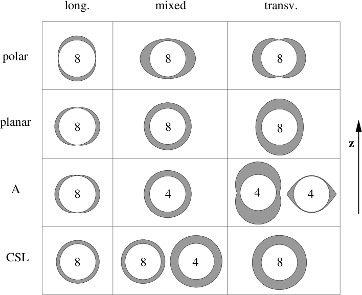
Abbildung 2.3: Schematic representation of the functions $\sqrt{\lambda_{r}}\phi_{0}$ occurring in the quasiparticle excitation energies, Eq. (2.38), for longitudinal, mixed, and transverse gaps in four different spin-one color-superconducting phases. All functions are symmetric with respect to rotations around the $z$-axis. The numbers correspond to the degeneracies of the respective excitation branch. In each case there are 12 excitation branches, from which we only show the gapped ones.

In the first line of Fig. 2.3 we show the angular structure of the gap in the polar phase. In the longitudinal case (first column), the gap vanishes at the equator of the Fermi surface since $\sqrt{\lambda_{1}}=|\cos\theta|$, i.e., there is a nodal line. In the mixed phase, $\lambda_{1}$ does not depend on the angle $\theta$. Nevertheless, there is an anisotropy due to the exponential factor $\exp(-d)$, cf. Eqs. (2.41) and (2.115). This anisotropy is also indicated schematically in Fig. 2.3. In the case of a transverse gap, $\beta=1$, the gap function has nodal points at the north and south pole of the Fermi surface since $\sqrt{\lambda_{1}}=|\sin\theta|$.

In the planar phase, the longitudinal gap has point nodes, since $\sqrt{\lambda_{1}}=|\sin\theta|$, while in the transverse case the gap is nonvanishing for all angles, $\sqrt{\lambda_{1}}=\sqrt{(1+\cos^{2}\theta)}$. In the mixed case, the gap is isotropic, $\lambda_{1}=1$.

The results for the A phase are illustrated in the third row of Fig. 2.3. In the longitudinal case, the gap has two point nodes, identical to the planar phase. It is not surprising that this structure can also be found in the A phase of superfluid ³He (cf. Fig. 1.8 in the introduction). The reason for this is the similarity of the matrix ${\cal M}_{\bf k}$, Eq. (2.99), in the case $\beta=0$ with the corresponding ansatz for the gap matrix in superfluid ³He [22]. Therefore, all longitudinal gaps reproduce the nonrelativistic limit. The 3-vector $\mbox{\boldmath${\gamma}$}_{\perp}({\bf k})$, accounting for pairing of quarks with opposite chirality, is not present in nonrelativistic theories, wherefore the results presented in the second and third column of Fig. 2.3 can be considered as relativistic extensions of the first column.

The mixed gap in the A phase is isotropic (note that this case is the only one where the ungapped excitation has degeneracy eight), whereas the transverse case exhibits two different gap structures, one having point nodes at the north and south pole of the Fermi surface, one nonvanishing for all directions of the quark momentum. Of course, these structures cannot be seen in the nonrelativistic theory of the A phase in ³He.

In the CSL phase, the gaps in all three cases are isotropic. Again, the nonrelativistic case reproduces the result for the B phase in ³He, shown in Fig. 1.8.

$T_{c}/\phi_{0}^{2SC}$	longitudinal	mixed	transverse
polar	$e^{-6}$	$1.4\,e^{-21/4}$	$e^{-9/2}$
planar	$e^{-6}$	$e^{-21/4}$	$e^{-9/2}$
A	$e^{-6}$	$e^{-21/4}$	$e^{-9/2}$
CSL	$e^{-6}$	$e^{-5}$	$e^{-9/2}$

Tabelle 2.2: The critical temperature $T_{c}$ in units of $\phi_{0}^{\rm 2SC}$ for four different spin-one color superconductors and longitudinal, mixed, and transverse gaps.

In Table 2.2, we present the absolute value of the critical temperature in units of the 2SC gap, $\phi_{0}^{\rm 2SC}$. Then, $T_{c}$ simply is given by $\exp(-d)$, cf. Eq. (2.77). In the polar phase with a mixed gap, the critical temperature is given by the angular average of this term, cf. Eq. (2.78). With $\phi_{0}^{\rm 2SC}\sim$ 10 - 100 MeV, the critical temperature in a spin-one color superconductor is therefore of the order of 10 - 400 keV. Finally, we remark that the BCS relation (1.5) for the critical temperature is violated in the cases of the mixed CSL and the transverse A phases, which can be seen from Eq. (2.76). This violation, also present in the CFL phase, originates from the two-gap structure, i.e., two excitation branches with different, non-zero energy gaps.

2.2 Patterns of symmetry breaking

In this section, we discuss possible symmetry breaking patterns in a spin-one color superconductor. In other words, we present a systematic classification of theoretically possible superconducting phases. As explained in the introduction, a superconducting phase is mathematically described by a nonvanishing order parameter $\Delta$ that spontaneously breaks the original symmetry group $G$ of the system. Remember that $\Delta$ is an element of a representation of $G$. In the case of a spin-one color superconductor, this representation is given by the tensor product of the antisymmetric color antitriplet $[\bar{\bf 3}]_{c}^{a}$ and the symmetric spin triplet $[{\bf 3}]_{J}^{s}$, cf. Eq. 1.9 and Sec. 1.3.3,

$$\Delta\in[\bar{\bf 3}]_{c}^{a}\otimes[{\bf 3}]_{J}^{s}\,\,.$$ (2.148)

Therefore, $\Delta$ is, as in the case of superfluid ³He, a complex $3\times 3$ matrix. There is no nontrivial contribution from the flavor structure since we consider systems with only one quark flavor. In Sec. 1.2.2, it has been discussed that the order parameter breaks down the group $G$ to a residual (proper) subgroup $H\subseteq G$. This means that any transformation $g\in H$ leaves the order parameter invariant,

$$g(\Delta)=\Delta\,\,.$$ (2.149)

In the following, we investigate this invariance condition in order to determine all possible order parameters $\Delta$ and the corresponding residual groups $H$. The method we use in this section is motivated by the analogous one for the case of superfluid ³He [22]. Note that in the previous section $\Delta$ already has been introduced as a part of the gap matrix, cf. Eqs. (2.24) and (2.99). The specific structure of $\Delta$ has been used for four different spin-one color-superconducting phases, namely the polar, planar, A, and CSL phases. Therefore, we expect to recover these four phases (among others) in the following discussion.

Let us first elaborate on the mathematical contents of Eq. (2.149). From Sec. 1.3.3 we know that the relevant symmetry group in the case of a spin-one color superconductor is

$$G=SU(3)_{c}\times SU(2)_{J}\times U(1)_{em}\times U(1)_{B}\,\,,$$ (2.150)

where $SU(3)_{c}$ is the (local) color gauge group, $SU(2)_{J}$ the (global) spin group, $U(1)_{em}$ the (local) electromagnetic gauge group, and $U(1)_{B}$ the (global) baryon number conservation group. Here, we put “local” and “global” in parentheses because these properties of the symmetries are not essential for the following classification. They are of relevance only for the interpretation of the results. Without loss of generality, we can restrict ourselves to the group

$$G=G_{1}\times G_{2}\times G_{3}\,\,,$$ (2.151)

where

$$G_{1}=SU(3)_{c}\,\,,\qquad G_{2}=SU(2)_{J}\,\,,\qquad G_{3}=U(1)\,\,.$$ (2.152)

Since in the one-flavor case the transformations of both $U(1)_{em}$ and $U(1)_{B}$ correspond to a multiplication with a phase factor, we can reduce our following arguments to a single $U(1)$. The extension to both $U(1)$’s can be done straightforwardly at the end. After specifying the group $G$, we have to specify how $G$ acts on the order parameter in Eq. (2.149). To this end, we write an arbitrary group element $g\in G$ as (in this section, no confusion with the strong coupling constant $g$ is possible)

$$g=(g_{1},g_{2},g_{3})\,\,,$$ (2.153)

where

$$g_{1}=\exp(-ia_{m}T_{m}^{T})\,\,,\qquad g_{2}=\exp(ib_{n}J_{n})\,\,,\qquad g_{3}=\exp(2ic\bf{1})\,\,,$$ (2.154)

with real coefficients $a_{m}$ ($m=1,\ldots,8$), $b_{n}$ ($n=1,2,3$), and $c$. The Gell-Mann matrices $T_{m}$ generate the group $SU(3)_{c}$, and we have taken into account that the color representation is an antitriplet. The matrices $J_{n}$ are the same as in Eq. (2.99), where they served as the basis of the color antitriplet. Here, they are used as the generators of the spin group $SU(2)_{J}$. For the generator of $U(1)$ we choose $2\cdot{\bf 1}$, where ${\bf 1}$ is the $3\times 3$ unit matrix. The factor 2 accounts for the diquark nature of the order parameter. The transformation $g$ acts on the matrix ${\cal M}_{\bf k}$, defined in Eq. (2.99), in the following way (abbreviating the 3-vector $\kappa_{j}\equiv[\alpha\,\hat{k}_{j}+\beta\,\gamma_{\perp}^{j}({\bf k})]$, such that ${\cal M}_{\bf k}=J_{i}\Delta_{ij}\kappa_{j}$)

$$g({\cal M}_{\bf k}) = g_{3}\,(g_{1}J_{i})\,\Delta_{ij}\,(g_{2}\kappa_{j})$$ (2.155)

$$= g_{3}\,g_{1}^{ik}\,J_{k}\,\Delta_{ij}\,g_{2}^{j\ell}\,\kappa_{\ell}\,\,.$$

Therefore, since $J_{i}\otimes\kappa_{j}$ is a basis of the representation $[\bar{\bf 3}]_{c}^{a}\otimes[{\bf 3}]_{J}^{s}$, the matrix $\Delta$ transforms as

$$g(\Delta_{ij})=g_{3}\,g_{1}^{ki}\,\Delta_{k\ell}\,g_{2}^{\ell j}\,\,.$$ (2.156)

Then, using Eqs. (2.154), the infinitesimal transformations of $\Delta$ by $G$ are given by

$$g(\Delta)\simeq\Delta-a_{m}T_{m}\Delta+b_{n}\Delta J_{n}+2c\,\Delta\,\,,$$ (2.157)

where $T_{m}\Delta$ as well as $\Delta J_{n}$ are matrix products. The invariance condition for the order parameter (2.149) is thus equivalent to

$$-a_{m}T_{m}\Delta+b_{n}\Delta J_{n}+2c\,\Delta=0\,\,.$$ (2.158)

This matrix equation can be written as a system of nine equations for the nine complex entries $\Delta_{11},\ldots,\Delta_{33}$ of the matrix $\Delta$. In principle, one can find all possible symmetry breaking patterns and corresponding order parameters by setting the determinant of the coefficient matrix to zero. Then, each possibility to make the determinant vanish yields a set of conditions for the coefficients $a_{m}$, $b_{n}$, $c$, and it can be checked if these conditions correspond to a residual subgroub $H$. But since this is much too complicated, we proceed via investigating possible subgroups explicitly. In the following, we focus only on the continuous subgroups of $G$.

Let us start with subgroups $H$ that contain the smallest possible continuous group, $U(1)$, i.e.,

$$H=U(1)\times H^{\prime}\,\,,$$ (2.159)

where $H^{\prime}$ is a direct product of Lie groups. The residual $U(1)$ must be generated by a $3\times 3$ matrix $U$ which is a linear combination of the generators of $G$, i.e., in general,

$$U=a_{m}T_{m}+b_{n}J_{n}+2c{\bf 1}\,\,.$$ (2.160)

Let us restrict to linear combinations that involve one generator of each group $G_{1}$, $G_{2}$, $G_{3}$, for instance

$$U=a_{8}T_{8}+b_{3}J_{3}+2c{\bf 1}\,\,.$$ (2.161)

In order to find all possible order parameters, it is necessary to consider at least one more combination, namely $U=a_{2}T_{2}+b_{3}J_{3}+2c{\bf 1}$. We comment on these two choices of the residual generator below. With Eq. (2.161), the invariance condition

$$e^{iU}(\Delta)=\Delta$$ (2.162)

results in a system of nine equations, which can be discussed explicitly,

$$\left(-\frac{a_{8}}{2\sqrt{3}}+2c\right)\Delta_{11}+ib_{3}\Delta_{12} = 0\,\,,$$ (2.163a)

$$\left(-\frac{a_{8}}{2\sqrt{3}}+2c\right)\Delta_{12}-ib_{3}\Delta_{11} = 0\,\,,$$ (2.163b)

$$\left(-\frac{a_{8}}{2\sqrt{3}}+2c\right)\Delta_{13} = 0\,\,,$$ (2.163c)

$$\left(-\frac{a_{8}}{2\sqrt{3}}+2c\right)\Delta_{21}+ib_{3}\Delta_{22} = 0\,\,,$$ (2.163d)

$$\left(-\frac{a_{8}}{2\sqrt{3}}+2c\right)\Delta_{22}-ib_{3}\Delta_{21} = 0\,\,,$$ (2.163e)

$$\left(-\frac{a_{8}}{2\sqrt{3}}+2c\right)\Delta_{23} = 0\,\,,$$ (2.163f)

$$\left(-\frac{a_{8}}{\sqrt{3}}+2c\right)\Delta_{31}+ib_{3}\Delta_{32} = 0\,\,,$$ (2.163g)

$$\left(-\frac{a_{8}}{\sqrt{3}}+2c\right)\Delta_{32}-ib_{3}\Delta_{31} = 0\,\,,$$ (2.163h)

$$\left(-\frac{a_{8}}{\sqrt{3}}+2c\right)\Delta_{33} = 0\,\,.$$ (2.163i)

The corresponding coefficient matrix $A$ exhibits a block structure and the determinant thus factorizes into four sub-determinants. Therefore, we have to consider the equation

$$0={\rm det}A={\rm det}A_{1}\,{\rm det}A_{2}\,{\rm det}A_{3}\,{\rm det}A_{4}\,\,,$$ (2.164)

where

$${\rm det}A_{1} = \left[\left(-\frac{a_{8}}{2\sqrt{3}}+2c\right)^{2}-b_{3}^{2}\right]^{2}\,\,,$$ (2.165a)

$${\rm det}A_{2} = \left(-\frac{a_{8}}{2\sqrt{3}}+2c\right)^{2}\,\,,$$ (2.165b)

$${\rm det}A_{3} = \left(\frac{a_{8}}{\sqrt{3}}+2c\right)^{2}-b_{3}^{2}\,\,,$$ (2.165c)

$${\rm det}A_{4} = \frac{a_{8}}{\sqrt{3}}+2c\,\,.$$ (2.165d)

Now, one can systematically list all possibilities that yield a zero determinant of the coefficient matrix and thus allow for a nonzero order parameter. For convenience, let us introduce a normalization for the order parameter,

$${\rm Tr}(\Delta\Delta^{\dagger})=1\,\,.$$ (2.166)

1. ${\rm det}A_{1}=0$.

   Here we distinguish between the cases (i) where the two terms in the angular brackets of Eq. (2.165a) cancel each other and (ii) where they separately vanish.

   1. $a_{8}$, $c$ arbitrary, $b_{3}=-a_{8}/(2\sqrt{3})+2c$.

      Inserting these conditions for the coefficients into Eqs. (2.163)), one obtains for the order parameter matrix

      $$\Delta=\frac{1}{N}\left(\begin{array}[]{ccc}\Delta_{1}&i\Delta_{1}&0\\ \Delta_{2}&i\Delta_{2}&0\\ 0&0&0\end{array}\right)\,\,,$$ (2.167)

      where the factor $1/N$ with $N=(2|\Delta_{1}|^{2}+2|\Delta_{2}|^{2})^{1/2}$ accounts for the normalization (2.166). In this case, the order parameter contains two independent parameters $\Delta_{1}$ and $\Delta_{2}$. From this form of the order parameter, we can now determine the group $H^{\prime}$ in Eq. (2.159). Inserting $\Delta$ into Eq. (2.158) and using the fact that the parameters $\Delta_{1}$, $\Delta_{2}$ are independent of each other, one obtains the conditions

      $$a_{1}=\ldots=a_{7}=b_{1}=b_{2}=0\,\,,\quad\frac{1}{2\sqrt{3}}a_{8}+b_{3}-2c=0\,\,.$$ (2.168)

      Consequently,

      $$H=U(1)\times U(1)\,\,,$$ (2.169)

      since a vanishing coefficient in Eq. (2.168) translates to a “broken dimension” of $G$. For instance, $a_{1}=0$ means that $T_{1}$ does not occur in the generators of $H$, etc. The dimensions of the residual Lie group can be counted with the help of the number of the conditions for the coefficients. Since ${\rm dim}\,G={\rm dim}\,G_{1}+{\rm dim}\,G_{2}+{\rm dim}\,G_{3}=8+3+1=12$, and the number of conditions in Eqs. (2.168) is 10, we conclude ${\rm dim}\,H=2$, which is in agreement with Eq. (2.169). Or, in other words, there is an additional $U(1)$, i.e., $H^{\prime}=U(1)$ in Eq. (2.159) because the equation relating the three coefficients $a_{8}$, $b_{3}$, $c$ allows for two linear independent generators $U$ and $V$ which are linear combinations of the generators $T_{8}$, $J_{3}$, ${\bf 1}$. Note that $U$ and $V$ are not uniquely determined. One possible choice is

      $$U=T_{8}-\frac{1}{2\sqrt{3}}J_{3}\,\,,\qquad V=2J_{3}+{\bf 1}\,\,.$$ (2.170)

      Different order parameters are obtained from two subcases:

      First, one can impose the additional relation $c=-a_{8}/(2\sqrt{3})$ between the two coefficients that have been arbitrary above. Then, $b_{3}=-a_{8}\sqrt{3}/2$. These two conditions yield

      $$\Delta=\frac{1}{N}\left(\begin{array}[]{ccc}\Delta_{1}&i\Delta_{1}&0\\ \Delta_{2}&i\Delta_{2}&0\\ 0&0&\Delta_{3}\end{array}\right)\,\,,$$ (2.171)

      where $N=(2|\Delta_{1}|^{2}+2|\Delta_{2}|^{2}+|\Delta_{3}|^{2})^{1/2}$. In this case, Eq. (2.158) leads to 11 conditions for the coefficients $a_{m}$, $b_{n}$, $c$, which leaves a subgroup

      $$H=U(1)\,\,,$$ (2.172)

      generated by a linear combination of generators of all three original subgroups $G_{1}$, $G_{2}$, $G_{3}$,

      $$U=T_{8}-\frac{\sqrt{3}}{2}J_{3}-\frac{1}{2\sqrt{3}}{\bf 1}\,\,.$$ (2.173)

      Second, one can set one of the coefficients $a_{8}$, $c$ to zero. The condition $c=0$ does not yield a new case. But $a_{8}=0$, and consequently $b_{3}=2c$, has to be treated separately. In this case, Eqs. (2.163) yield

      $$\Delta=\frac{1}{N}\left(\begin{array}[]{ccc}\Delta_{1}&i\Delta_{1}&0\\ \Delta_{2}&i\Delta_{2}&0\\ \Delta_{3}&i\Delta_{3}&0\end{array}\right)\,\,,$$ (2.174)

      where $N=(2|\Delta_{1}|^{2}+2|\Delta_{2}|^{2}+2|\Delta_{3}|^{2})^{1/2}$. The residual group is given by

      $$H=U(1)\,\,,$$ (2.175)

      generated by

      $$U=2J_{3}+{\bf 1}\,\,.$$ (2.176)

   2. $c=a_{8}/(4\sqrt{3})$, $b_{3}=0$.

      Here, one obtains

      $$\Delta=\frac{1}{N}\left(\begin{array}[]{ccc}\Delta_{1}&\Delta_{2}&\Delta_{3}\\ \Delta_{4}&\Delta_{5}&\Delta_{6}\\ 0&0&0\end{array}\right)\,\,,$$ (2.177)

      where $N=(\sum_{i=1}^{6}|\Delta_{i}|^{2})^{1/2}$. Again, the residual group is one-dimensional,

      $$H=U(1)\,\,,$$ (2.178)

      generated by

      $$U=T_{8}+\frac{1}{4\sqrt{3}}{\bf 1}\,\,.$$ (2.179)

2. ${\rm det}A_{2}=0$.

   This determinant vanishes in the following cases:

   1. $b_{3}$ arbitrary, $c=a_{8}/(4\sqrt{3})$.

      With Eqs. (2.163), one obtains

      $$\Delta=\frac{1}{N}\left(\begin{array}[]{ccc}0&0&\Delta_{1}\\ 0&0&\Delta_{2}\\ 0&0&0\end{array}\right)\,\,,$$ (2.180)

      where $N=(|\Delta_{1}|^{2}+|\Delta_{2}|^{2})^{1/2}$. Inserting $\Delta$ into Eq. (2.158) yields

      $$a_{1}=\ldots=a_{7}=b_{1}=b_{2}=0\,\,,\quad c=\frac{1}{4\sqrt{3}}a_{8}\,\,.$$ (2.181)

      As for the order parameter (2.167), the residual group is given by

      $$H=U(1)\times U(1)\,\,.$$ (2.182)

      However, the corresponding generators differ from those in Eqs. (2.170),

      $$U=T_{8}+\frac{1}{4\sqrt{3}}{\bf 1}\,\,,\qquad V=J_{3}\,\,.$$ (2.183)

   2. $b_{3}$ arbitrary, $a_{8}=c=0$.

      In this case,

      $$\Delta=\frac{1}{N}\left(\begin{array}[]{ccc}0&0&\Delta_{1}\\ 0&0&\Delta_{2}\\ 0&0&\Delta_{3}\end{array}\right)\,\,,$$ (2.184)

      where $N=(|\Delta_{1}|^{2}+|\Delta_{2}|^{2}+|\Delta_{3}|^{2})^{1/2}$. The residual group is

      $$H=U(1)\,\,,$$ (2.185)

      which is a subgroup of the spin group $G_{2}=SU(2)_{J}$, since it is generated by

      $$U=J_{3}\,\,.$$ (2.186)

3. ${\rm det}A_{3}=0$.

   1. $a_{8}$, $c$ arbitrary, $b_{3}=a_{8}/\sqrt{3}+2c$.

      In this case, we find with Eqs. (2.163),

      $$\Delta=\frac{1}{\sqrt{2}}\left(\begin{array}[]{ccc}0&0&0\\ 0&0&0\\ 1&i&0\end{array}\right)\,\,.$$ (2.187)

      This matrix differs from all previously discussed order parameters in that it is uniquely determined. Here, as in all cases above, we omitted a possible phase factor which could multiply $\Delta$ without violating the normalization. In Eq. (2.187) we recover the A phase, which already has been introduced in Eq. (1.8h) for superfluid ³He and in Eq. (2.122) for a spin-one color superconductor. Inserting $\Delta$ into Eqs. (2.158) yields the following relations,

      $$a_{4}=\ldots=a_{7}=b_{1}=b_{2}=0\,\,,\quad\frac{1}{\sqrt{3}}a_{8}-b_{3}+2c=0\,\,.$$ (2.188)

      Consequently, besides the relation between $a_{8}$, $b_{3}$, and $c$, there are only 6 additional conditions. Thus, the dimension of the residual group is $12-7=5$. We obtain

      $$H=SU(2)\times U(1)\times U(1)\,\,,$$ (2.189)

      where $SU(2)$ is generated by $2T_{1}$, $2T_{2}$, $2T_{3}$, and thus is a subgroup of the color gauge group $G_{1}=SU(3)_{c}$. The factor 2 accounts for the validity of the $SU(2)$ commutation relations,

      $$[J_{i},J_{j}]=i\,\epsilon_{ijk}J_{k}\,\,,\qquad i,j,k\leq 3\,\,.$$ (2.190)

      For the generators of the two $U(1)$’s one can choose

      $$U=T_{8}-\frac{1}{2\sqrt{3}}{\bf 1}\,\,,\qquad V=J_{3}+{\bf 1}\,\,.$$ (2.191)

      As in case 1.(i), there is a subcase that produces an additional order parameter. Namely, if we require the condition $c=a_{8}/(4\sqrt{3})$, which yields $b_{3}=\sqrt{3}\,a_{8}/2$, we obtain

      $$\Delta=\frac{1}{N}\left(\begin{array}[]{ccc}0&0&\Delta_{2}\\ 0&0&\Delta_{3}\\ \Delta_{1}&i\Delta_{1}&0\end{array}\right)\,\,,$$ (2.192)

      where $N=(2|\Delta_{1}|^{2}+|\Delta_{2}|^{2}+|\Delta_{3}|^{2})^{1/2}$. From Eq. (2.163) we conclude that all other coefficients vanish. Consequently,

      $$H=U(1)\,\,,$$ (2.193)

      with the generator

      $$U=T_{8}+\frac{\sqrt{3}}{2}J_{3}+\frac{1}{4\sqrt{3}}{\bf 1}\,\,.$$ (2.194)

   2. $b_{3}=0$, $c=-a_{8}/(2\sqrt{3})$.

      With Eqs. (2.163) one obtains

      $$\Delta=\frac{1}{N}\left(\begin{array}[]{ccc}0&0&0\\ 0&0&0\\ \Delta_{1}&\Delta_{2}&\Delta_{3}\end{array}\right)\,\,,$$ (2.195)

      where $N$ is defined as in Eq. (2.184). From Eq. (2.158) we conclude in this case

      $$a_{4}=\ldots=a_{7}=b_{1}=b_{2}=b_{3}=0\,\,,\quad c=-\frac{a_{8}}{2\sqrt{3}}\,\,.$$ (2.196)

      Hence, the residual group is

      $$H=SU(2)\times U(1)\,\,,$$ (2.197)

      generated by $2T_{1}$, $2T_{2}$, $2T_{3}$, and

      $$U=T_{8}-\frac{1}{2\sqrt{3}}{\bf 1}\,\,.$$ (2.198)

4. ${\rm det}A_{4}=0$.

   There are two cases in which ${\rm det}A_{4}=0$:

   1. $b_{3}$ arbitrary, $c=-a_{8}/(2\sqrt{3})$.

      These relations lead to

      $$\Delta=\left(\begin{array}[]{ccc}0&0&0\\ 0&0&0\\ 0&0&1\end{array}\right)\,\,,$$ (2.199)

      As in the A phase, Eq. (2.187), the order parameter is uniquely determined. It describes the polar phase, which has been studied in the previous section. Inserting the order parameter of the polar phase into the invariance condition, Eq. (2.158), yields

      $$a_{4}=\ldots=a_{7}=b_{1}=b_{2}=0\,\,,\quad c=-\frac{1}{2\sqrt{3}}a_{8}\,\,.$$ (2.200)

      Therefore, the residual group is

      $$H=SU(2)\times U(1)\times U(1)$$ (2.201)

      with the generators $2T_{1}$, $2T_{2}$, $2T_{3}$, and

      $$U=T_{8}-\frac{1}{2\sqrt{3}}{\bf 1}\,\,,\qquad V=J_{3}\,\,.$$ (2.202)

      Thus, the symmetry breaking pattern in the polar phase is similar to that in the A phase, cf. (2.191). But while in the A phase both residual $U(1)$’s are combinations of the original symmetries, in the polar phase one of them is a subgroup of $G_{2}=SU(2)_{J}$.

   2. $b_{3}$ arbitrary, $a_{8}=c=0$.

      This case is identical to case 2.(ii).

As mentioned above, one also has to take into account generators of a residual $U(1)$ where $T_{8}$ in Eq. (2.161) is replaced by $T_{2}$, i.e.,

$$U=a_{2}T_{2}+b_{3}J_{3}+2c{\bf 1}\,\,.$$ (2.203)

The reason why $T_{2}$ plays a special role is that we used the generator $J_{3}$ of the spin group, which is proportional to $T_{2}$. Consequently, we expect to find additional residual groups that connect the color group with the spin group (meaning a residual $U(1)$ generated by a combination of a color and a spin generator). The calculations with this generator are completely analogous to the ones with the ansatz (2.161). Therefore, without presenting the details, let us mention that the ansatz (2.203) yields one new unique order parameter, namely

$$\Delta=\frac{1}{\sqrt{2}}\left(\begin{array}[]{ccc}1&0&0\\ 0&1&0\\ 0&0&0\end{array}\right)\,\,.$$ (2.204)

This order parameter corresponds to the planar phase, introduced in Eq. (2.116). In this case, Eq. (2.158) yields

$$a_{1}=0\,\,,\quad a_{3}=a_{4}=\ldots=a_{7}=b_{1}=b_{2}=0\,\,,\quad a_{2}=2b_{3}\,\,,\quad c=\frac{1}{4\sqrt{3}}a_{8}\,\,.$$ (2.205)

Thus, the residual group is

$$H=U(1)\times U(1)\,\,,$$ (2.206)

with the generators

$$U=2T_{2}+J_{3}\,\,,\qquad V=T_{8}+\frac{1}{4\sqrt{3}}\,{\bf 1}\,\,.$$ (2.207)

Let us now turn to possible groups $H$ that do not contain any $U(1)$ but solely consist of higher-dimensional Lie groups, say

$$H=SU(2)\times H^{\prime}\,\,.$$ (2.208)

Let $U_{1}$, $U_{2}$, $U_{3}$ be the generators of the residual $SU(2)$. They are linear combinations of the generators of $G$,

$$U_{1} = a^{1}_{m}T_{m}+b^{1}_{n}J_{n}+2c^{1}{\bf 1}\,\,,$$ (2.209a)

$$U_{2} = a^{2}_{m}T_{m}+b^{2}_{n}J_{n}+2c^{2}{\bf 1}\,\,,$$ (2.209b)

$$U_{3} = a^{3}_{m}T_{m}+b^{3}_{n}J_{n}+2c^{3}{\bf 1}\,\,.$$ (2.209c)

Since they must fulfill the $SU(2)$ commutation relations, Eq. (2.190), they must not contain the generator of $G_{3}=U(1)$, the unit matrix, i.e., $c^{1}=c^{2}=c^{3}=0$ . Therefore, there are three possibilities. First, each $U_{i}$ is a combination of color and spin generators. Second and third, each $U_{i}$ is composed solely of color or spin generators, respectively. The simplest options to realize these cases are

$$(a)\qquad U_{i}=T_{i}^{\prime}+J_{i}\,\,,$$ (2.210a)

$$(b)\qquad U_{i}=T_{i}^{\prime}\,\,,$$ (2.210b)

$$(c)\qquad U_{i}=J_{i}\,\,,$$ (2.210c)

where $(T_{1}^{\prime},T_{2}^{\prime},T_{3}^{\prime})$ is either given by $(2T_{1},2T_{2},2T_{3})$ or $(2T_{7},-2T_{5},2T_{2})$, which both fulfill the required commutation relations. Using the options $(a)$, $(b)$, $(c)$, let us first show that $H^{\prime}$ in Eq. (2.208) cannot be a second $SU(2)$. To this end, assume that $H^{\prime}=SU(2)$ with generators $V_{1}$, $V_{2}$, $V_{3}$, which have the same form as the generators $U_{i}$ in Eqs. (2.210). Then, since the Lie algebra of $H$ is a direct sum of the constituent Lie algebras, cf. Sec. 1.2.2, we have to require

$$[U_{i},V_{j}]=0\,\,.$$ (2.211)

This condition reduces all options to one, namely

$$U_{i}=T_{i}^{\prime}\,\,,\qquad V_{i}=J_{i}$$ (2.212)

(or vice versa). However, now the invariance equation for the order parameter yields

$$\Delta J_{i}=0\,\,,$$ (2.213)

for all $i=1,2,3$, which does not allow for a nonzero order parameter $\Delta$. Therefore, $H^{\prime}=SU(2)$ is forbidden. Since the cases with $H^{\prime}=U(1)$ and $H^{\prime}=U(1)\times U(1)$ were already covered in the above discussion, the only possibility that is left is $H^{\prime}={\bf 1}$ and thus $H=SU(2)$.

From Eqs. (2.210), case $(c)$ can be immediately excluded since it also leads to Eq. (2.213). The same argument excludes case $(b)$ with $(T_{1}^{\prime},T_{2}^{\prime},T_{3}^{\prime})=(2T_{7},-2T_{5},2T_{2})$. Case $(b)$ with $(T_{1}^{\prime},T_{2}^{\prime},T_{3}^{\prime})=(2T_{1},2T_{2},2T_{3})$ leads to two order parameters already considered above, namely the A phase, Eq. (2.187), and the polar phase, Eq. (2.199). In case $(a)$, only $(T_{1}^{\prime},T_{2}^{\prime},T_{3}^{\prime})=(2T_{7},-2T_{5},2T_{2})$ is possible. With

$$U_{i}\Delta=-T_{i}^{\prime}\Delta+\Delta J_{i}=0\,\,,$$ (2.214)

one finds

$$\Delta=\frac{1}{\sqrt{3}}\left(\begin{array}[]{ccc}1&0&0\\ 0&1&0\\ 0&0&1\end{array}\right)\,\,.\\$$ (2.215)

Indeed, it can be checked with Eq. (2.158) that this order parameter leads to

$$a_{1}=a_{3}=a_{4}=a_{6}=a_{8}=c=0\,\,,\quad a_{2}=2b_{3}\,\,,\quad a_{5}=-2b_{2}\,\,,\quad a_{7}=2b_{1}\,\,,$$ (2.216)

which corresponds to $H=SU(2)$, consisting of joint rotations in color and spin space. This is the CSL phase introduced for a spin-one color superconductor in Eq. (2.129) and for superfluid ³He (therein called B phase) in Eq. (1.8d).

Finally, we give an argument why an even larger subgroup, i.e., an $SU(3)$, cannot occur in the residual group $H$. Assume that there are eight generators $W_{1},\ldots,W_{8}$ of this $SU(3)$. Then, as for the $SU(2)$ subgroup above, there can be no contribution to $W_{1},\ldots,W_{8}$ from the $G_{3}$ generator due to the $SU(3)$ commutation relations for the generators,

$$[W_{i},W_{j}]=i\,f_{ijk}W_{k}\,\,,\qquad i,j,k\leq 8\,\,,$$ (2.217)

where $f_{ijk}$ are the $SU(3)$ structure constants. Also, $W_{i}=T_{i}$ is excluded because in this case the invariance condition yields $T_{8}\Delta=0$ and thus $\Delta=0$. Therefore, at least one of the spin generators has to be included. For instance, choose $W_{8}=T_{8}+b_{3}J_{3}$. Then, from the commutation relation $[W_{4},W_{5}]\sim W_{8}$ we conclude that also $J_{1}$ and $J_{2}$ must be included via $W_{4}=T_{4}+b_{1}J_{1}$ and $W_{5}=T_{5}+b_{2}J_{2}$. But now the three equations $W_{4}\Delta=W_{5}\Delta=W_{8}\Delta=0$ lead to $\Delta=0$. Therefore, we conclude that there is no residual group $H$ that contains an $SU(3)$. For a more rigorous proof one has to take into account more complicated linear combinations of the original generators.

Before we summarize and interpret the results, let us add two remarks.

First, we explain how the above discussion can be extended to two original $U(1)$ symmetries, one accounting for electromagnetism (local) and one for baryon number conservation (global). Denoting the generators of these two groups by $2q\,{\bf 1}_{em}$ and $2\cdot{\bf 1}_{B}$, respectively, where $q$ is the electric charge of the quark, it is very simple to generalize the results to this situation. For instance, in the polar phase there are not only two residual $U(1)$’s generated by $U=T_{8}-1/(2\sqrt{3}){\bf 1}$ and $V=J_{3}$, cf. Eqs. (2.202), but three $U(1)$’s generated by $U_{1}=T_{8}-1/(2q\sqrt{3}){\bf 1}_{em}$ (local!), $U_{2}=T_{8}-1/(2\sqrt{3}){\bf 1}_{B}$ (global!), and $V=J_{3}$. The extension in the other phases works analogously. Note that the same problem in a two- or three-flavor color superconductor is less trivial. In these cases, the generator of the electromagnetic gauge group is not proportional to the unit matrix since it involves different electric charges of the respective quark flavors.

The second remark concerns the difference between the uniquely determined order parameters, such as those for the polar, planar, A, and CSL phases, and the ones that depend on one or more free parameters. Without elaborating on the group-theoretical details, let us refer to the analogous situation in ³He. In this case, all order parameters of the first kind lead to so-called “inert” states [22]. All experimentally known states of superfluid ³He belong to this class of order parameters. Mathematically speaking, these order parameter matrices play a special role due to a theorem (“Michel’s Theorem”) [22, 118], which ensures that these order parameters correspond to a stationary point of any $G$-invariant functional of $\Delta$ (for instance the effective potential). This is the reason why in Secs. 2.1, 2.3, and 2.4 we focus on these order parameters.

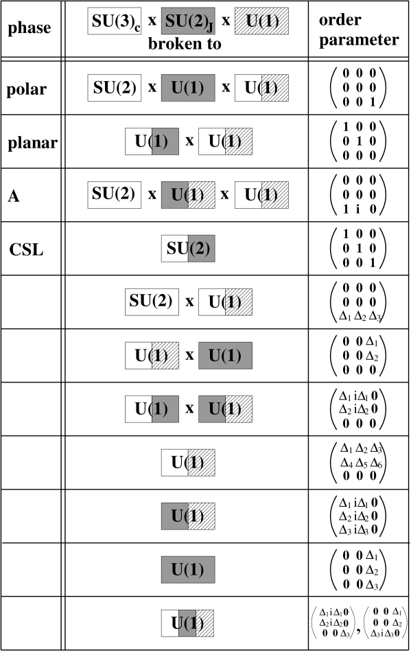
Abbildung 2.4: Symmetry breaking patterns and order parameters for a spin-one color superconductor. The original symmetry group (first line) is given by the color gauge group $SU(3)_{c}$ (blank background), the spin group $SU(2)_{J}$ (grey background), and a $U(1)$ (hatched background). The latter can be regarded as the electromagnetic gauge group or the baryon number conservation group. The backgrounds of the residual groups illustrate the symmetry breaking pattern. For instance, the blank $SU(2)$ occuring in the residual group of the polar phase is generated solely by generators of the original $SU(3)_{c}$ while the blank/hatched $U(1)$ in the same line is generated by a linear combination of the generators of the original $SU(2)_{J}$ and $U(1)$ groups. For the explicit expression of these generators, see text.

In Fig. 2.4, we summarize our results in a list of all superconducting phases that we have found in the above discussion. It should be mentioned that this list is not complete, since for the generators of the residual $U(1)$’s we have restricted ourselves to two special forms given in Eqs. (2.161) and (2.203). Therefore, there are certainly more (at least noninert) order parameters that lead to an allowed symmetry breaking. The inert states are listed in the first four lines. Each of these four states has its analogue in superfluid ³He [22]. Note that the ${\rm A}_{1}$ phase, which is experimentally observed in ³He in the presence of an external magnetic field (see the phase diagram in Fig. 1.4), does not lead to an allowed symmetry breaking in the case of a spin-one color superconductor [62]. To see this, one inserts the corresponding order parameter from Eq. (1.8l) into Eq. (2.158). One obtains

$$a_{1}=a_{3}=b_{1}=b_{2}=0\,\,,\quad a_{4}=a_{7}\,\,,\quad a_{5}=a_{6}\,\,,\quad\frac{1}{2}a_{2}+\frac{1}{2\sqrt{3}}a_{8}-b_{3}-2c=0\,\,.$$ (2.218)

These 7 conditions suggest that ${\rm dim}\,H=12-7=5$ and thus $H=SU(2)\times U(1)\times U(1)$. However, there is no possibility to construct three generators from the above conditions that fulfill the commutation relations (2.190). For instance, assume that two of these generators are given by $U_{1}=T_{4}+T_{7}$ and $U_{2}=T_{5}+T_{6}$. Then, with Eq. (2.217), $[U_{1},U_{2}]\sim T_{3}$. But since $a_{3}=0$, the third generator $U_{3}$ cannot be proportional to $T_{3}$. Consequently, there is no ${\rm A}_{1}$ phase in a spin-one color superconductor.

Below the four inert states we list the eight noninert states which have been found above. Note that one of these noninert phases, given in Eq. (2.195), has a larger residual symmetry group than the planar and CSL phases.

There are several properties of the spin-one phases which can easily be read off from Fig. 2.4. First, consider the spin group $SU(2)_{J}$. This symmetry accounts for the rotational symmetry in real space of the normal-conducting phase (remember that, in the case of the spin-one representation, one can equivalently consider $SO(3)_{J}$ instead of $SU(2)_{J}$). The list shows that spatial symmetry is broken in each case. For instance, in the polar phase, $SU(2)_{J}$ is broken to its subgroup $U(1)_{J}$. Therefore, the superconducting phase is invariant under rotations around one fixed axis in real space. This axis (the 3-axis) is chosen by the spins of the Cooper pairs which all are aligned in one direction. In the previous section it has been shown that this breakdown of the rotational symmetry leads to an anisotropy of the energy gap. In most of the other cases, the breaking of the spatial rotation symmetry is more subtle: For instance in the planar phase, the superconducting state is invariant under a special joint rotation in color and real space. Note that in the planar phase, unlike the polar phase, the special role of the third spatial direction originates from the fact that the spins are aligned perpendicular to the 3-axis. The most interesting breakdown of spatial symmetries is present in the CSL phase. Here, any rotation in real space leaves the system invariant as long as one simultaneously performes the same rotation in fundamental color space which is spanned by the three directions red, green, and blue. This special form of locking of color and spatial indices is responsible for the fact that the CSL phase (and the B phase in ³He) is “pseudoisotropic”. In fact, in the previous section it has been shown that there is no anisotropy in the gap function, cf. Fig. 2.3.

Next, let us read off some properties concerning the color symmetry. It is obvious that in none of the cases the full color symmetry is preserved. In this sense, it is justified to call each phase a color superconductor. In three of the cases, there is a residual color subgroup $SU(2)$, namely in the polar phase, the A phase, and the noninert phase given by Eq. (2.195). Mathematically speaking, this residual group originates from the fact that the order parameter has only nonzero elements in its third row. Therefore, the third direction in fundamental color space is preferred. Physically, this means that the Cooper pairs carry color charge anti-blue, or, in other words, only red and green quarks form Cooper pairs. Of course, the choice of the anti-blue direction is convention; more generally speaking, quarks of one color remain unpaired. Remember that this is also true for the 2SC phase in a two-flavor color superconductor, cf. Sec. 1.3.1.

From Sec. 1.3.2 we know that a spontaneously broken gauge symmetry is equivalent to massive gauge bosons. In the case of a color superconductor, these masses are the magnetic screening masses of the gluons. Therefore, in the cases where there is a residual color subgroup $SU(2)$, we expect a Meissner effect for five of the eight gluons. Three of the gluons, however, namely those corresponding to the generators $T_{1}$, $T_{2}$, $T_{3}$, do not attain a Meissner mass. This is also obvious from the fact that these gluons do not see the (anti-)blue color charge which is carried by the Cooper pairs. For a more detailed and quantitative discussion of the color Meissner effect, see the next section. Also with respect to the breakdown of the color symmetry, the CSL phase is exceptional. Although there is a residual $SU(2)$, where three of the color generators are involved, we expect all eight gluons to attain a Meissner mass. To this end, note that this residual $SU(2)$ is a global symmetry and therefore all dimensions of the gauge group have to be considered as broken. This is analogous to the CFL phase introduced in Sec. 1.3.1. In this three-flavor color-superconducting phase, color is locked to flavor which results in a color Meissner effect for all eight gluons.

In order to discuss the question whether the color superconductors in Fig. 2.4 are also electromagnetic superconductors, one regards the $U(1)$ of the original symmetry (hatched background in the figure) as the electromagnetic gauge group $U(1)_{em}$. From ordinary superconductors, cf. Sec. 1.2.1, we know that this symmetry is spontaneously broken below the critical temperature. Therefore, a simple conclusion is that all states in the list without a hatched background occurring in the residual group are electromagnetic superconductors. Obviously, this is the case for the CSL phase and for one of the noninert states, defined in Eq. (2.184). This is a remarkable result because electromagnetic superconductivity is absent in both spin-zero superconductors that were discussed in the introduction. Moreover, the presence of the electromagnetic Meissner effect in a spin-one color superconductor probably leads to observable implications for the properties of a neutron star [100].

In most of the phases listed in Fig. 2.4, the question of the electromagnetic Meissner effect is less trivial. Although in none of the cases the electromagnetic gauge group is untouched, there are residual groups that involve the $U(1)_{em}$ generator. Here we have to distinguish between two cases. First, $U(1)_{em}$ may only be coupled to the global spin group which results in a global residual (sub)group. In this case we expect the photon to attain a magnetic screening mass since this situation is analogous to the CFL (and CSL) phase(s), where a coupling of the gluons to the global flavor (spin) symmetry leads to a color Meissner effect for all gluons. Second, $U(1)_{em}$ may couple to the color gauge group. This happens for instance in the polar, planar, and A phases. Since this scenario exactly corresponds to the cases of the 2SC and CFL phases, we expect a “rotated” magnetic photon (cf. Sec. 1.3.2) that can penetrate the superconductor (= no electromagnetic Meissner effect). Besides the color Meissner effect, also the electromagnetic Meissner effect is treated quantitatively in Sec. 2.3. In this section, we also discuss the case of a many-flavor system in which each quark flavor separately forms spin-one Cooper pairs in the polar phase. It turns out that in this case there is an electromagnetic Meissner effect, in spite of the apparently contradicting conclusion from Fig. 2.4.

Finally, let us comment on the superfluidity of the phases. To this end, regard the hatched $U(1)$ as the particle number conservation symmetry $U(1)_{B}$. As discussed in the introduction, a spontaneous breakdown of this symmetry leads to superfluidity (= a stable superflow and vortices in a rotating system). Again, the only phases in the list, where the breakdown of this symmetry is obvious, are the CSL phase and the phase from Eq. (2.184). In all other cases, the question of superfluidity is nontrivial. It is comparable to the A phase in ³He, see discussion in Sec. 1.2.2. Remember that in the CFL phase, $U(1)_{B}$ is completely broken, cf. Eq. (1.12), which renders this phase a superfluid, contrary to the 2SC phase, cf. Eq. (1.11), which behaves similar to most of the spin-one phases (e.g., the polar phase) and is no superfluid. In Sec. 1.1.2, it has been indicated that also the question of superfluidity is of great physical relevance, since superfluid vortices (together with magnetic flux tubes) play an important role for possible explanations of the properties of a neutron star.

2.3 Mixing and screening of photons and gluons

From the previous section, where symmetry breaking patterns in a spin-one color superconductor have been studied, we know that different color-superconducting phases have different properties with respect to electromagnetic and color fields, i.e., with respect to photons and gluons. With the help of simple group-theoretical arguments it has been shown that for instance the CSL phase exhibits an electromagnetic Meissner effect. This is in contrast to the 2SC and CFL phases in a spin-zero color superconductor. In these phases there is a color Meissner effect for five and eight gluons, respectively, but due to a locking of the color and electromagnetic gauge groups there is no electromagnetic Meissner effect. In Sec. 1.3.2, it was mentioned that this absence of the Meissner effect is somehow related to a mixing of the gauge boson fields and that this is analogous to what happens in the Weinberg-Salam model of electroweak interactions.

It is the goal of this section to clarify this mixing between photons and gluons, which is also expected to be present in several spin-one phases, cf. Fig. 2.4. Furthermore, we not only present a calculation of the magnetic screening masses (= Meissner masses) in order to quantitatively verify the group-theoretical predictions from the last section, but also compute the electric screening masses (= Debye masses) for all gauge bosons. The calculations are shown for four different color-superconducting phases. We consider the 2SC and CFL phases as well as the polar and CSL phases. More precisely, for the spin-one phases we focus on the “mixed polar” and the “mixed CSL” phases, cf. explanation below Eq. (2.99), but refer to them shortly as “polar” and “CSL” phases

This section is organized as follows. In Sec. 2.3.1 we start from the QCD partition function for massless quarks in the presence of gluon and photon gauge fields in order to derive the gauge boson propagators in a color superconductor. This fundamental study provides the basis for the following sections, since it can be applied for arbitrary phases in color superconductivity. It is also general in the sense that we consider gauge fields for arbitrary four-momenta $P$ while afterwards we focus on the limiting case $P\to 0$ in order to discuss screening of static and homogeneous electric and magnetic fields.

In Sec. 2.3.2, we present a general definition of the mixing angle. This mixing angle is the analogue of the Weinberg angle, cf. Table 1.1, and quantitatively describes the mixing between photons and gluons. Its definition is based on the results of Sec. 2.3.1. Making use of the results of the group-theoretical study in Sec. 2.2, the explicit form of the mixing angle in terms of the strong and electromagnetic coupling constants $g$ and $e$ is presented for the above mentioned four color-superconducting phases.

In the next sections we extend the results of Sec. 2.3.2 by performing a calculation of the Debye and Meissner masses for all gauge bosons. These masses correspond to the inverse screening lengths for electric and magnetic fields, respectively. They are obtained from the longitudinal and transverse components of the polarization tensors in the zero-energy, low-momentum limit. In the first of these sections, Sec. 2.3.3, we perform all calculations that do not depend on the special color-superconducting phase. A part of these calculations, namely the integrals over the absolute value of the quark momentum, are deferred to Appendix E. In Sec. 2.3.4, we specify the results for the above mentioned phases, i.e., we derive the particular expressions for the relevant components of the polarization tensors. Readers who are not interested in the technical details may skip this section. All results and a discussion are given in Sec. 2.3.5. We present all screening masses for photons and gluons which yield the mixing angles and the masses for the (physically relevant) mixed, or “rotated”, gauge bosons. One of the points we discuss in this section is in which cases these mixing angles obtained from the calculation of the screening masses differ from the ones obtained in Sec. 2.3.2.

2.3.1 Gluon and photon propagators

In the following, we provide the theoretical basis for the calculation of the Debye and Meissner masses in a color superconductor. The results of this section are the final form for gluon and photon propagators, Eq. (2.254), and the definitions for the “rotated” Debye and Meissner masses, Eqs. (2.255).

As in Sec. 2.1.1, where the QCD gap equation has been derived, we start from the QCD partition function for massless quarks. (In Sec. 2.1.1, the quark mass $m$ was kept for the derivation of the gap equation, but was set to zero before the explicit calculations were performed.) Besides the gluon fields $A_{a}^{\mu}$, however, we also include a photon field $A^{\mu}$,

$${\cal Z}=\int{\cal D}A\,e^{S_{A}}{\cal Z}_{q}[A]\,\,.$$ (2.219)

Since the emphasis of this section is put on the gauge fields, we choose a slightly different notation compared to Eq. (2.1). The action for gluon and photon fields is given by $S_{A}$. It consists of three parts, cf. also Eq. (2.2),

$$S_{A}=S_{F^{2}}+S_{gf}+S_{FPG}\,\,,$$ (2.220)

where $S_{gf}$ and $S_{FPG}$ are the gauge fixing and ghost terms, respectively, and

$$S_{F^{2}}\equiv-\frac{1}{4}\int_{X}(F_{a}^{\mu\nu}F^{a}_{\mu\nu}+F^{\mu\nu}F_{\mu\nu})$$ (2.221)

is the gauge field part. The space-time integration is defined as in Sec. 2.1.1. The field strength tensors $F^{a}_{\mu\nu}=\partial_{\mu}A_{\nu}^{a}-\partial_{\nu}A_{\mu}^{a}+gf^{abc}A_{\mu}^{b}A_{\nu}^{c}$ correspond to the gluon fields $A_{\mu}^{a}$, while $F_{\mu\nu}=\partial_{\mu}A_{\nu}-\partial_{\nu}A_{\mu}$ corresponds to the photon field $A_{\mu}$. The functional ${\cal Z}_{q}[A]$ is the grand partition function of massless quarks in the presence of gluon and photon fields and a chemical potential $\mu$. It is given by

$${\cal Z}_{q}[A]=\int{\cal D}\bar{\psi}\,{\cal D}\psi\exp\left[\int_{X}\bar{\psi}\,(i\,\gamma^{\mu}\partial_{\mu}+\mu\gamma_{0}+g\,\gamma^{\mu}A_{\mu}^{a}T_{a}+e\,\gamma^{\mu}A_{\mu}Q)\,\psi\right]\,\,,$$ (2.222)

where $T_{a}$ are the generators in the fundamental representation of the gauge group of strong interactions, $SU(3)_{c}$, and $Q$ is the generator of the electromagnetic $U(1)_{em}$. Here, $Q$ is not necessarily proportional to the unit matrix (as it was the case in Sec. 2.2), since in the current general treatment the number of flavors is not specified. The coupling constants for the strong interaction and electromagnetism are denoted by $g$ and $e$, respectively. The quark fields $\psi$ are spinors in color, flavor, and Dirac space.

In order to take into account Cooper pairing of the quarks, we include a diquark source term. This has been done for instance in Refs. [46, 119]. We generalize this treatment by also taking into account the photon field. Then, after integrating out the fermion fields, the partition function is given by [119]

$${\cal Z}=\int{\cal D}A\exp\left[S_{A}+\frac{1}{2}{\rm Tr}\,\ln({\cal S}^{-1}+A_{\mu}^{a}\hat{\Gamma}^{\mu}_{a})\right]\,\,,$$ (2.223)

where the trace runs over space-time, Nambu-Gor’kov, color, flavor, and Dirac indices. The sum over $a$ now runs from 1 to 9, where $A_{\mu}^{9}\equiv A_{\mu}$ is the photon field. ${\cal S}\equiv{\cal S}(X,Y)$ is the quasiparticle propagator in Nambu-Gor’kov space. We also defined the $2\times 2$ Nambu-Gor’kov matrices

$$\hat{\Gamma}_{a}^{\mu}\equiv{\rm diag}\left(\Gamma_{a}^{\mu},\overline{\Gamma}_{a}^{\mu}\right)\equiv\left\{\begin{array}[]{lll}{\rm diag}(g\,\gamma^{\mu}T_{a},-g\,\gamma^{\mu}T_{a}^{T})&\mbox{for}&\quad a=1,\ldots,8\,\,,\\ \\ {\rm diag}(e\,\gamma^{\mu}Q,-e\,\gamma^{\mu}Q)&\mbox{for}&\quad a=9\,\,.\end{array}\right.$$ (2.224)

For convenience, we included the coupling constants into $\Gamma_{a}^{\mu}$ and $\overline{\Gamma}_{a}^{\mu}$, although it differs from the notation introduced in Sec. 2.1, see Eq. (2.10).

In Eq. (2.223), we did not explicitly keep the fluctuations of the order parameter field, cf. Eq. (26) of Ref. [119]. This is possible, since we are only interested in the gauge field propagator. Nevertheless, it should be kept in mind that, like in any theory with spontaneously broken gauge symmetry, these fluctuations mix with the (4-)longitudinal (unphysical) components of the gauge field. As usual, using a suitable choice of ’t Hooft gauge, the fluctuations can be decoupled from the gauge field. Then, in unitary gauge, one finds that the gauge field propagator is explicitly (4-)transverse [119], in accordance with general principles [120, 121].

Expanding the logarithm in Eq. (2.223) to second order in the gauge fields, we obtain

$$\frac{1}{2}{\rm Tr}\,\ln({\cal S}^{-1}+A_{\mu}^{a}\hat{\Gamma}^{\mu}_{a})\simeq\frac{1}{2}{\rm Tr}\,\ln{\cal S}^{-1}+\frac{1}{2}\,{\rm Tr}[A_{\mu}^{a}\,\hat{\Gamma}_{a}^{\mu}\,{\cal S}]-\frac{1}{4}{\rm Tr}[A_{\mu}^{a}\,\hat{\Gamma}_{a}^{\mu}\,{\cal S}\,A_{\nu}^{b}\,\hat{\Gamma}_{b}^{\nu}\,{\cal S}]\,\,.$$ (2.225)

Following Ref. [119], the sum of all terms which are quadratic in the gauge fields will be denoted by $S_{2}$. $S_{2}$ does not only contain the pure gluon and photon terms but also two terms which mix gluon and photon fields. In order to perform the trace over space-time, we introduce the Fourier transforms

$${\cal S}(X,Y) = \frac{T}{V}\sum_{K}e^{-iK\cdot(X-Y)}{\cal S}(K)\,\,,$$ (2.226a)

$$A_{\mu}^{a}(X) = \sum_{P}e^{-iP\cdot X}A_{\mu}^{a}(P)\,\,,$$ (2.226b)

where we used translational invariance, ${\cal S}(X,Y)={\cal S}(X-Y)$. Then we obtain

$$S_{2} = -\frac{1}{4}\int_{X,Y}{\rm Tr}[A_{\mu}^{a}(X)\,\hat{\Gamma}_{a}^{\mu}\,{\cal S}(X,Y)\,A_{\nu}^{b}(Y)\,\hat{\Gamma}_{b}^{\nu}\,{\cal S}(Y,X)]$$ (2.227)

$$= -\frac{1}{4}\sum_{K,P}{\rm Tr}[A_{\mu}^{a}(-P)\,\hat{\Gamma}_{a}^{\mu}\,{\cal S}(K)\,A_{\nu}^{b}(P)\,\hat{\Gamma}_{b}^{\nu}\,{\cal S}(K-P)]$$

$$= -\frac{1}{2}\frac{V}{T}\sum_{P}A_{\mu}^{a}(-P)\,\Pi_{ab}^{\mu\nu}(P)\,A_{\nu}^{b}(P)\,\,,$$

where the trace now runs over Nambu-Gor’kov, color, flavor, and Dirac indices and where we defined the polarization tensor

$$\Pi_{ab}^{\mu\nu}(P)\equiv\frac{1}{2}\frac{T}{V}\sum_{K}{\rm Tr}[\hat{\Gamma}_{a}^{\mu}\,{\cal S}(K)\,\hat{\Gamma}_{b}^{\nu}\,{\cal S}(K-P)]\,\,.$$ (2.228)

The Nambu-Gor’kov quasiparticle propagator in momentum space ${\cal S}(K)$ is defined as in Eq. (2.18),

$${\cal S}(K)=\left(\begin{array}[]{cc}G^{+}(K)&\Xi^{-}(K)\\ \Xi^{+}(K)&G^{-}(K)\end{array}\right)\,\,.$$ (2.229)

In the following, we may put the regular self-energies $\Sigma^{\pm}$ to zero since, to the order we are computing, they do not influence the results for the polarization tensors. Consequently,

$$G^{\pm}(K) = \left\{[G_{0}^{\pm}]^{-1}(K)-\Phi^{\mp}(K)\,G_{0}^{\mp}(K)\,\Phi^{\pm}(K)\right\}^{-1}\,\,,$$ (2.230a)

$$\Xi^{\pm}(K) = -G_{0}^{\mp}(K)\Phi^{\pm}(K)G^{\pm}(K)\,\,,$$ (2.230b)

where $G_{0}^{\pm}(K)=(\gamma_{\mu}K^{\mu}\pm\mu\gamma_{0})^{-1}$ is the free propagator. The gap matrices $\Phi^{\pm}(K)$ are given by Eqs. (2.23) and (2.24). The quasiparticle propagators are

$$G^{\pm}(K)=[G_{0}^{\mp}(K)]^{-1}\sum_{e=\pm}\sum_{r=1,2}{\cal P}^{r}_{\bf k}\,\Lambda_{\bf k}^{\mp e}\,\frac{1}{k_{0}^{2}-\left[\epsilon_{k,r}^{e}(\phi^{e})\right]^{2}}\,\,.$$ (2.231)

In Sec. 2.1, only $G^{+}$ was needed, cf. Eq. (2.36). In order to derive the corresponding expression for $G^{-}$, we used the identity $\gamma_{0}{\cal M}_{\bf k}^{\dagger}{\cal M}_{\bf k}\gamma_{0}={\cal M}_{\bf k}{\cal M}_{\bf k}^{\dagger}$. This identity is valid in the phases we consider, i.e., the 2SC, CFL, polar, and CSL phases. (However, in the A phase it does not hold, which causes a slight modification of the above result, cf. Sec. 2.4.) All quantities in Eq. (2.231) are defined as in Sec. 2.1, i.e., ${\cal P}^{r}_{\bf k}$ are projectors onto the eigenspaces of the hermitian matrix $L_{\bf k}=\gamma_{0}{\cal M}_{\bf k}^{\dagger}{\cal M}_{\bf k}\gamma_{0}$. In all phases considered here, there are two eigenvalues of this matrix, denoted by $\lambda_{1}$ and $\lambda_{2}$. They appear in the quasiparticle excitation energies

$$\epsilon_{k,r}^{e}(\phi^{e})\equiv\left[(\mu-ek)^{2}+\lambda_{r}|\phi^{e}|^{2}\right]^{1/2}\,\,.$$ (2.232)

The projectors are given by Eq. (2.35). The anomalous propagators can be written as

$$\Xi^{+}(K) = -\sum_{e,r}\gamma_{0}{\cal M}_{\bf k}\gamma_{0}\,{\cal P}^{r}_{\bf k}\,\Lambda_{\bf k}^{-e}\,\frac{\phi^{e}(K)}{k_{0}^{2}-\left[\epsilon_{k,r}^{e}(\phi^{e})\right]^{2}}\,\,,$$ (2.233a)

$$\Xi^{-}(K) = -\sum_{e,r}{\cal M}_{\bf k}^{\dagger}\,{\cal P}^{r}_{\bf k}\,\Lambda_{\bf k}^{e}\,\frac{\phi^{e\,*}(K)}{k_{0}^{2}-\left[\epsilon_{k,r}^{e}(\phi^{e})\right]^{2}}\,\,.$$ (2.233b)

As in Ref. [119], we introduce a set of complete, orthogonal projectors for each 4-vector $P^{\mu}=(p_{0},{\bf p})$,

$${\cal Q}_{1}^{\mu\nu}\equiv g^{\mu\nu}-{\cal Q}_{2}^{\mu\nu}-{\cal Q}_{3}^{\mu\nu}\,\,,\qquad{\cal Q}_{2}^{\mu\nu}\equiv\frac{N^{\mu}N^{\nu}}{N^{2}}\,\,,\qquad{\cal Q}_{3}^{\mu\nu}\equiv\frac{P^{\mu}P^{\nu}}{P^{2}}\,\,.$$ (2.234)

With $N^{\mu}\equiv(p_{0}p^{2}/P^{2},p_{0}^{2}{\bf p}/P^{2})$, the projector ${\cal Q}_{2}^{\mu\nu}$ projects onto the one-dimensional subspace that is (4-)orthogonal to $P^{\mu}$ but (3-)parallel to ${\bf p}$. The operator ${\cal Q}_{3}^{\mu\nu}$ projects onto the one-dimensional subspace parallel to $P^{\mu}$. Consequently, ${\cal Q}_{1}^{\mu\nu}$ projects onto a two-dimensional subspace that is (4-)orthogonal to both $P^{\mu}$ and $N^{\mu}$. Furthermore, this subspace is (3-)orthogonal to ${\bf p}$. With the additional tensor

$${\cal Q}_{4}^{\mu\nu}=N^{\mu}P^{\nu}+P^{\mu}N^{\nu}$$ (2.235)

we can decompose the polarization tensor [121],

$$\Pi^{\mu\nu}_{ab}(P)=\sum_{i}\Pi^{i}_{ab}(P)\,{\cal Q}_{i}^{\mu\nu}\,\,.$$ (2.236)

(In the notation of Refs. [119, 121], ${\cal Q}_{1}\equiv{\rm A},{\cal Q}_{2}\equiv{\rm B},{\cal Q}_{3}\equiv{\rm E},{\cal Q}_{4}\equiv{\rm C}$.) Since for $i=1,2,3$, ${\cal Q}_{i}^{\mu\nu}{\cal Q}_{4\nu\mu}=0$, the coefficients $\Pi^{i}_{ab}(P)$ of the projection operators are given by

$$\Pi^{i}_{ab}(P)=\frac{\Pi^{\mu\nu}_{ab}(P){\cal Q}_{i\nu\mu}}{{\cal Q}_{i\lambda}^{\lambda}}\quad,\qquad i=1,2,3\,\,.$$ (2.237)

The remaining coefficient corresponding to ${\cal Q}_{4}$ is

$$\Pi^{4}_{ab}(P)=\frac{\Pi_{ab}^{\mu\nu}(P){\cal Q}_{4\nu\mu}}{{\cal Q}_{4}^{\lambda\sigma}{\cal Q}_{4\sigma\lambda}}\,\,.$$ (2.238)

The explicit forms for $\Pi^{i}_{ab}(P)$ are given in Ref. [119], Eqs. (42) and (43). Employing the decomposition of the polarization tensor in Eq. (2.227), we obtain

$$S_{2} = -\frac{1}{2}\frac{V}{T}\sum_{P}\sum_{i}A_{\mu}^{a}(-P){\cal Q}_{i}^{\mu\nu}\Pi_{ab}^{i}(P)A_{\nu}^{b}(P)\,\,.$$ (2.239)

Now we add the free gauge field term

$$S^{(0)}_{F^{2}}=-\frac{1}{2}\frac{V}{T}\sum_{P}A_{\mu}^{a}(-P)(P^{2}g^{\mu\nu}-P^{\mu}P^{\nu})A_{\nu}^{a}(P)=-\frac{1}{2}\frac{V}{T}\sum_{P}A_{\mu}^{a}(-P)P^{2}({\cal Q}_{1}^{\mu\nu}+{\cal Q}_{2}^{\mu\nu})A_{\nu}^{a}(P)\,\,.$$ (2.240)

We obtain

$$S_{2}+S^{(0)}_{F^{2}}=-\frac{1}{2}\frac{V}{T}\sum_{P}A_{\mu}^{a}(-P)\left\{\sum_{i=1}^{2}{\cal Q}_{i}^{\mu\nu}\left[\delta_{ab}P^{2}+\Pi_{ab}^{i}(P)\right]+\sum_{i=3}^{4}{\cal Q}_{i}^{\mu\nu}\Pi_{ab}^{i}(P)\right\}A_{\nu}^{b}(P)\,\,.$$ (2.241)

Since we finally want to read off the gluon and photon propagators, we have to transform this expression in two ways. First, concerning the Dirac structure it is necessary to get rid of the term proportional to ${\cal Q}_{4}$ which mixes the longitudinal mode (3-parallel to ${\bf p}$) with the unphysical mode (4-parallel to $P^{\mu}$). Then, inverting the inverse propagator becomes trivial, because it is just a linear combination of the complete, orthogonal projectors ${\cal Q}_{1},{\cal Q}_{2},{\cal Q}_{3}$. Second, in order to obtain the physical modes we have to diagonalize the resulting $9\times 9$ matrices which, after eliminating ${\cal Q}_{4}$, will replace $\delta_{ab}P^{2}+\Pi_{ab}^{i}(P)$, $i=1,2$, and $\Pi_{ab}^{i}(P)$, $i=3,4$ in Eq. (2.241).

We first write $S_{2}+S^{(0)}_{F^{2}}$ as

$$S_{2}+S^{(0)}_{F^{2}} = -\frac{1}{2}\frac{V}{T}\sum_{P}\Big{\{}\sum_{i=1}^{2}A_{i}^{a\mu}(-P)\left[\delta_{ab}P^{2}+\Pi_{ab}^{i}(P)\right]A^{b}_{i\mu}(P)+A_{3}^{a\mu}(-P)\Pi_{ab}^{3}(P)A^{b}_{3\mu}(P)$$ (2.242)

$$\hskip 59.75095pt+\;A_{2}^{a\mu}(-P)N_{\mu}\Pi^{4}_{ab}(P)P_{\nu}A_{3}^{b\nu}(P)$$

$$\hskip 59.75095pt+\;A_{3}^{a\mu}(-P)P_{\mu}\Pi^{4}_{ab}(P)N_{\nu}A_{2}^{b\nu}(P)\Big{\}}\,\,,$$

where $A_{i}^{a\mu}(P)\equiv{\cal Q}_{i}^{\mu\nu}A_{\nu}^{a}(P)$ are the gauge fields projected on the subspace corresponding to ${\cal Q}_{i}$. Now one can “unmix” the fields $A_{2}^{\mu}(P)$ and $A_{3}^{\mu}(P)$ by the following transformation of the unphysical field component $A^{a}_{3\mu}(P)$, which does not affect the final result since we integrate over all fields in the partition function,

$$A_{3}^{a\mu}(-P) \longrightarrow A_{3}^{a\mu}(-P)-A_{2}^{c\nu}(-P)N_{\nu}\Pi^{4}_{cb}(P)\left[\Pi^{3}(P)\right]^{-1}_{ba}\,P^{\mu}\,\,,$$ (2.243a)

$$A^{a}_{3\mu}(P) \longrightarrow A^{a}_{3\mu}(P)-P_{\mu}\left[\Pi^{3}(P)\right]^{-1}_{ab}\Pi^{4}_{bc}(P)\,N_{\nu}A_{2}^{c\nu}(P)\,\,.$$ (2.243b)

After this transformation, one is left with quadratic expressions in the projected fields. The transformation modifies the term corresponding to $i=2$,

$$S_{2}+S^{(0)}_{F^{2}} = -\frac{1}{2}\frac{V}{T}\sum_{P}A_{\mu}^{a}(-P)\Big{(}{\cal Q}_{1}^{\mu\nu}\left[\delta_{ab}P^{2}+\Pi_{ab}^{1}(P)\right]$$ (2.244)

$$+\;{\cal Q}_{2}^{\mu\nu}\left\{\delta_{ab}P^{2}+\Pi_{ab}^{2}(P)-P^{2}N^{2}\Pi^{4}_{ac}(P)\,\left[\Pi^{3}(P)\right]^{-1}_{cd}\,\Pi^{4}_{db}(P)\right\}$$

$$+\;{\cal Q}_{3}^{\mu\nu}\Pi^{3}_{ab}(P)\Big{)}A^{b}_{\nu}(P)\,\,.$$

Before we do the diagonalization in the 9-dimensional gluon-photon space, we add the gauge fixing term $S_{gf}$. We choose the following gauge with gauge parameter $\lambda$,

$$S_{gf}=-\frac{1}{2\lambda}\frac{V}{T}\sum_{P}A_{\mu}^{a}(-P)P^{\mu}P^{\nu}A_{\nu}^{a}(P)=-\frac{1}{2\lambda}\frac{V}{T}\sum_{P}A_{\mu}^{a}(-P)P^{2}{\cal Q}_{3}^{\mu\nu}A_{\nu}^{a}(P)\,\,.$$ (2.245)

This looks like a covariant gauge but, including the fluctuations of the order parameter, which we did not write explicitly, it is actually some kind of ’t Hooft gauge, cf. Eq. (50) of Ref. [119]. Moreover, had we fixed the gauge prior to the shift (2.243) of the gauge fields, we would have to start with an expression which is non-local and also involves the (3-)longitudinal components $A_{2}^{a\mu}$ of the gauge field.

Adding the gauge fixing term (2.245) to Eq. (2.244) leads to

$$S_{2}+S^{(0)}_{F^{2}}+S_{gf}=-\frac{1}{2}\frac{V}{T}\sum_{P}\sum_{i=1}^{3}A^{a}_{\mu}(-P){\cal Q}_{i}^{\mu\nu}\Theta^{i}_{ab}(P)A^{b}_{\nu}(P)\,\,,$$ (2.246)

with

$$\Theta^{i}_{ab}(P)\equiv\left\{\begin{array}[]{cl}\delta_{ab}P^{2}+\Pi_{ab}^{1}(P)&\mbox{for}\quad i=1\,\,,\\ \\ \delta_{ab}P^{2}+\Pi_{ab}^{2}(P)-P^{2}N^{2}\Pi^{4}_{ac}(P)\,\left[\Pi^{3}(P)\right]^{-1}_{cd}\,\Pi^{4}_{db}(P)&\mbox{for}\quad i=2\,\,,\\ \\ \delta_{ab}\frac{1}{\lambda}P^{2}+\Pi^{3}_{ab}(P)&\mbox{for}\quad i=3\,\,.\end{array}\right.$$ (2.247)

In order to obtain the physical modes, we have to diagonalize the $9\times 9$ matrices $\Theta^{i}_{ab}(P)$. Since $\Theta^{i}_{ab}(P)$ is real and symmetric, diagonalization is achieved via an orthogonal transformation with a $9\times 9$ matrix ${\cal O}_{i}(P)$,

$$S_{2}+S^{(0)}_{F^{2}}+S_{gf}=-\frac{1}{2}\frac{V}{T}\sum_{P}\sum_{i=1}^{3}\tilde{A}_{\mu,i}^{a}(-P){\cal Q}_{i}^{\mu\nu}\tilde{\Theta}_{aa}^{i}(P)\tilde{A}_{\nu,i}^{a}(P)\,\,,$$ (2.248)

where

$$\tilde{A}_{\mu,i}^{a}(P)={\cal O}_{i}^{ab}(P)A_{\mu}^{b}(P)$$ (2.249)

are the rotated gauge fields and

$$\tilde{\Theta}_{aa}^{i}(P)={\cal O}_{i}^{ab}(P)\Theta^{i}_{bc}(P){\cal O}_{i}^{ac}(P)$$ (2.250)

are diagonal matrices. The index $i$ in $\tilde{A}^{a}_{\mu,i}$ has a different origin than in $A^{a}_{i\mu}$ introduced in Eq. (2.242). For $\tilde{A}^{a}_{\mu,i}$, it indicates that for each $i=1,2,3$ one has to perform a separate diagonalization. For $A^{a}_{i\mu}$ it denoted the projection corresponding to the projector ${\cal Q}_{i}^{\mu\nu}$.

Note that the orthogonal matrix ${\cal O}_{i}(P)$ depends on $P^{\mu}$. For energies and momenta much larger than the superconducting gap parameter the polarization tensor is explicitly (4-)transverse, $\Pi^{3}=0$, and diagonal in $a,b$. In this case, ${\cal O}_{i}(P)\to{\bf 1}$. Consequently, the gauge fields are not rotated. However, in the limit $p_{0}=0$, $p\to 0$ it is known that gluons and photons mix at least in the 2SC and CFL phases, cf. Sec. 1.3.2 and references therein, ${\cal O}_{i}(P)\neq{\bf 1}$. Thus, the mixing angle between gluons and photons, which will be discussed in Sec. 2.3.2, is in general a function of $P^{\mu}$ and interpolates between a nonvanishing value at $p_{0}=0$, $p\to 0$ and zero when $p_{0},p\to\infty$. Note also that the orthogonal matrix ${\cal O}_{i}(P)$ depends on $i$, i.e., it may be different for longitudinal and transverse modes. We comment on this in more detail below.

From Eq. (2.248), we can immediately read off the inverse propagator for gluons and photons. It is

$${\Delta^{-1}}_{aa}^{\mu\nu}(P)=\sum_{i=1}^{3}{\cal Q}_{i}^{\mu\nu}\tilde{\Theta}_{aa}^{i}(P)\,\,.$$ (2.251)

From the definition of $\tilde{\Theta}_{aa}^{i}(P)$ we conclude

$$\tilde{\Theta}^{i}_{aa}(P)\equiv\left\{\begin{array}[]{cl}P^{2}+\tilde{\Pi}_{aa}^{i}(P)&\mbox{for}\quad i=1,2\,\,,\\ \\ \frac{1}{\lambda}P^{2}+\tilde{\Pi}^{3}_{aa}(P)&\mbox{for}\quad i=3\,\,,\end{array}\right.$$ (2.252)

where

$$\tilde{\Pi}_{aa}^{i}(P)=\left\{\begin{array}[]{cl}{\cal O}_{i}^{ab}(P)\Pi^{i}_{bc}(P){\cal O}_{i}^{ac}(P)&\mbox{for}\quad i=1,3\,\,,\\ \\ {\cal O}_{2}^{ab}(P)\left\{\Pi_{bc}^{2}(P)-P^{2}N^{2}\Pi^{4}_{bd}(P)\,\left[\Pi^{3}(P)\right]^{-1}_{de}\,\Pi^{4}_{ec}(P)\right\}{\cal O}_{2}^{ac}(P)&\mbox{for}\quad i=2\,\,.\end{array}\right.$$ (2.253)

In the case $p_{0}=0$, using Eqs. (42) and (43) of Ref. [119] one realizes that the extra term involving $\Pi^{3}$ and $\Pi^{4}$ for $i=2$ vanishes. Thus, in this case one only has to diagonalize the original polarization tensors $\Pi^{i}_{ab}$.

Finally, we end up with the gauge boson propagator

$$\Delta_{aa}^{\mu\nu}(P)=\frac{1}{P^{2}+\tilde{\Pi}_{aa}^{1}(P)}{\cal Q}_{1}^{\mu\nu}+\frac{1}{P^{2}+\tilde{\Pi}_{aa}^{2}(P)}{\cal Q}_{2}^{\mu\nu}+\frac{\lambda}{P^{2}+\lambda\tilde{\Pi}_{aa}^{3}(P)}{\cal Q}_{3}^{\mu\nu}\,\,.$$ (2.254)

Setting the gauge parameter $\lambda=0$, we are left with the transverse and (3-)longitudinal modes, in accordance with general principles [120, 121]. The static color and electromagnetic properties of the color superconductor are characterized by the Debye masses $\tilde{m}_{D,a}$ and the Meissner masses $\tilde{m}_{M,a}$ which are defined as

$$\tilde{m}^{2}_{D,a} \equiv -\lim\limits_{p\to 0}\tilde{\Pi}_{aa}^{2}(0,{\bf p})=-\lim\limits_{p\to 0}\tilde{\Pi}_{aa}^{00}(0,{\bf p})\,\,,$$ (2.255a)

$$\tilde{m}^{2}_{M,a} \equiv -\lim\limits_{p\to 0}\tilde{\Pi}_{aa}^{1}(0,{\bf p})=\frac{1}{2}\lim\limits_{p\to 0}(\delta^{ij}-\hat{p}^{i}\hat{p}^{j})\tilde{\Pi}_{aa}^{ij}(0,{\bf p})\,\,.$$ (2.255b)

Since the orthogonal matrices ${\cal O}_{i}(P)$ are regular in the limit $p_{0}=0$, $p\to 0$, the masses can also be obtained by first computing $\lim_{p\to 0}\Pi_{ab}^{\mu\nu}(0,{\bf p})$ and then diagonalizing the resulting $9\times 9$ mass matrix. In Sec. 2.3.3, we use this method to compute $\tilde{m}^{2}_{D,a}$ and $\tilde{m}^{2}_{M,a}$, since the diagonalization of the matrix $\Pi_{ab}^{\mu\nu}(P)$ for arbitrary $P^{\mu}$ is too difficult.

2.3.2 The mixing angle

In this section, we investigate the structure of the orthogonal matrices ${\cal O}_{i}(P)$ which diagonalize the gauge field part of the grand partition function. In general, the matrices ${\cal O}_{i}(P)$ mix all gluon components among themselves and with the photon. However, in the limit $p_{0}=0$, $p\to 0$ it turns out that the only non-zero off-diagonal elements of the tensor $\Pi_{ab}^{i}\equiv\lim_{p\to 0}\Pi_{ab}^{i}(0,{\bf p})$ are $\Pi_{89}^{i}=\Pi_{8\gamma}^{i}=\Pi_{\gamma 8}^{i}$. Physically speaking, gluons do not mix among themselves and only the eighth gluon mixes with the photon. In this case, Eq. (2.253) reduces to the diagonalization of a $2\times 2$ matrix. Consequently, the diagonalization is determined by only one parameter $\theta_{i}$ and the (nontrivial part of the) transformation operator reads

$${\cal O}_{i}=\left(\begin{array}[]{cc}\cos\theta_{i}&\sin\theta_{i}\\ -\sin\theta_{i}&\cos\theta_{i}\end{array}\right)\,\,.$$ (2.256)

The new fields are

$$\tilde{A}^{8}_{\mu,i} = \cos\theta_{i}\,A^{8}_{\mu}+\sin\theta_{i}\,A_{\mu}\,\,,$$ (2.257a)

$$\tilde{A}_{\mu,i} = -\sin\theta_{i}\,A^{8}_{\mu}+\cos\theta_{i}\,A_{\mu}\,\,.$$ (2.257b)

The new polarization functions (eigenvalues of $\Pi_{ab}^{i}$) are

$$\tilde{\Pi}_{88}^{i} = \Pi_{88}^{i}\cos^{2}\theta_{i}+2\Pi_{8\gamma}^{i}\sin\theta_{i}\cos\theta_{i}+\Pi^{i}_{\gamma\gamma}\sin^{2}\theta_{i}\,\,,$$ (2.258a)

$$\tilde{\Pi}^{i}_{\gamma\gamma} = \Pi_{88}^{i}\sin^{2}\theta_{i}-2\Pi_{8\gamma}^{i}\sin\theta_{i}\cos\theta_{i}+\Pi^{i}_{\gamma\gamma}\cos^{2}\theta_{i}\,\,.$$ (2.258b)

The mixing angle $\theta_{i}$ is given by

$$\tan 2\theta_{i}=\frac{2\Pi_{8\gamma}^{i}}{\Pi_{88}^{i}-\Pi^{i}_{\gamma\gamma}}\,\,.$$ (2.259)

If $[\Pi_{8\gamma}^{i}]^{2}=\Pi_{88}^{i}\Pi^{i}_{\gamma\gamma}$, the determinant of $\Pi_{ab}^{i}$ is zero, which means that there is a vanishing eigenvalue. In this case, we have

$$\cos^{2}\theta_{i}=\frac{\Pi_{88}^{i}}{\Pi_{88}^{i}+\Pi_{\gamma\gamma}^{i}}\,\,,$$ (2.260)

and the new polarization tensors, Eqs. (2.258), have the simple form

$$\tilde{\Pi}_{88}^{i}=\Pi_{88}^{i}+\Pi^{i}_{\gamma\gamma}\quad,\qquad\tilde{\Pi}^{i}_{\gamma\gamma}=0\,\,.$$ (2.261)

Physically, a vanishing polarization tensor for the rotated photon corresponds to the absence of the electromagnetic Meissner effect for $i=1$, or the absence of Debye screening for $i=2$.

Next, we show how to determine the specific mixing angles from the results of Sec. 2.2. In an ordinary superconductor, the Meissner effect and thus a non-vanishing Meissner mass $m_{M,\gamma}$ originate from a non-zero electric charge of a Cooper pair. Besides this magnetic screening there is also electric screening of photons described by the photon Debye mass $m_{D,\gamma}$. Of course, in a color superconductor, in addition to the electric charge we also have to take into account the color charge. The group-theoretical method from Sec. 2.2 allows us to investigate whether there exists a (new) charge which generates an unbroken symmetry. In this case, a Cooper pair is neutral with respect to this charge, and consequently one expects that there is neither a Meissner effect nor Debye screening. The new charge is a linear combination of electric and color charges. Correspondingly, the associated gauge field is a linear combination of the photon and the eighth gluon field, which, in turn, defines the mixing angle. The group-theoretical method only allows to identify a new charge, and thus does not distinguish between electric Debye or magnetic Meissner screening. Consequently, the mixing angles for longitudinal (electric) and transverse (magnetic) modes deduced by this method are identical, $\theta_{1}=\theta_{2}\equiv\theta$.

From Sec. 2.2 we know that in the polar phase (and in several other spin-one phases) there is a residual symmetry group $U(1)$ generated by a linear combination of the generators $Q\equiv 2q$ of $U(1)_{em}$ and $T_{8}$ of $SU(3)_{c}$. Let us denote this residual group by $\tilde{U}(1)_{em}$ and the corresponding generator by $\tilde{Q}$. In general, the new charge generator is given by

$$\tilde{Q}=Q+\eta\,T_{8}\,\,,$$ (2.262)

where $\eta$ is a real coefficient. For instance, in the polar phase, cf. Eqs. (2.202), $\eta=-2\sqrt{3}q$. In Table 2.3, we list the relevant quantities regarding the spontaneous breakdown of the gauge symmetries $SU(3)_{c}\times U(1)_{em}$. The results for the polar and CSL phases are taken from Sec. 2.2. Note that in the case of the CSL phase, there is no nontrivial residual gauge group. The only residual symmetry is global, cf. Fig. 2.4. The corresponding results for the spin-zero phases can be found using exactly the same method as presented in Sec. 2.2, see Refs. [55, 56, 57, 58, 101]. The respective charge generators $Q={\rm diag}(q_{1},\ldots,q_{N_{f}})$ are defined by the electric charges of the quark flavors. With $q_{1}=2/3$, $q_{2}=q_{3}=-1/3$ for $u$, $d$, and $s$ quarks, the charge generators shown in the table apply to a system with $u$ and $d$ quarks (2SC) and a system with $d$, $s$, and $u$ quarks (CFL).

	Q	generators of	$\eta$
		residual gauge group
2SC	diag$(2/3,-1/3)$	$T_{1},T_{2},T_{3},Q+\eta T_{8}$	$-1/\sqrt{3}$
CFL	diag$(-1/3,-1/3,2/3)\,\,$	$Q+\eta T_{8}$	$2/\sqrt{3}$
CSL	$2q$	0	–
polar	$2q$	$\,\,T_{1},T_{2},T_{3},Q+\eta T_{8}\,\,$	$\,\,-2\sqrt{3}\,q\,\,$

Tabelle 2.3: Charge generators $Q$, generators of the residual gauge group, and coefficients $\eta$ for all color-superconducting phases considered in this section. For the CSL and polar phases, the electric charge of the quark is denoted by $q$.

In order to deduce the mixing angle $\theta$, we rewrite the covariant derivative, $D_{\mu}=\partial_{\mu}-igA_{\mu}^{a}T_{a}-ieA_{\mu}Q$, in terms of the new charge generator $\tilde{Q}$ and the linearly independent generator

$$\tilde{T}_{8}=T_{8}+\lambda Q\,\,,$$ (2.263)

which belongs to the broken part of the group; $\lambda$ is a real constant to be determined below. We also have to replace the gauge fields $A_{\mu}^{8}$ and $A_{\mu}$ by the rotated fields (2.257) and the associated coupling constants $g$, $e$ by new coupling constants $\tilde{g}$, $\tilde{e}$. Thus, we demand the identity [55, 56, 58]

$$gA_{\mu}^{8}T_{8}+eA_{\mu}Q=\tilde{g}\tilde{A}_{\mu}^{8}\tilde{T}_{8}+\tilde{e}\tilde{A}_{\mu}\tilde{Q}\,\,.$$ (2.264)

Inserting Eqs. (2.257) for the rotated fields and the definitions of $\tilde{Q}$ and $\tilde{T}_{8}$ we determine

$$\tilde{g}=g\cos\theta\quad,\qquad\tilde{e}=e\cos\theta\quad,\qquad\lambda=-\eta\frac{e^{2}}{g^{2}}\,\,,$$ (2.265)

and the mixing angle

$$\cos^{2}\theta=\frac{g^{2}}{g^{2}+\eta^{2}e^{2}}\,\,.$$ (2.266)

Since $g\gg e$, the mixing angle in all three cases is small. Thus, according to Eqs. (2.257), the gluon almost remains a gluon and the photon almost remains a photon and therefore it is justified to call the rotated gauge bosons the new gluon and the new photon.

In the 2SC, CFL, and polar phases, the new charge is neither Debye- nor Meissner-screened. We therefore expect that the polarization tensor for the rotated photon vanishes in the zero-energy, zero-momentum limit,

$$\tilde{\Pi}_{\gamma\gamma}^{1,2}=0\,\,.$$ (2.267)

As we shall see in the following section, this argument is not quite correct for the 2SC and polar phases, as it neglects the effect of the unpaired blue quarks on the screening of electric and magnetic fields. In the CSL phase, on the other hand, there is no residual $\tilde{U}(1)_{em}$ symmetry and we conclude that all gauge fields experience the Meissner effect and Debye screening, since in this case there does not exist any charge with respect to which a Cooper pair is neutral. Concerning color screening, one concludes from Table 2.3, that in the 2SC phase and the polar phase only the gluons 4-8 are screened while in the CFL and CSL phases all gluons are screened (see also discussion in Sec. 2.2).

2.3.3 Calculation of the polarization tensors

In this section, we calculate the polarization tensors $\Pi_{ab}^{\mu\nu}(P)$ given in Eq. (2.228) in the limit $p_{0}=0$, $p\to 0$. In this case, the Debye and Meissner masses, cf. Eqs. (2.255), are obtained from the coefficients of the first two projectors in the decomposition (2.236). They will be calculated in the next section. Here, we first derive a general expression for the polarization tensor that holds for all different phases. Then we insert the order parameters of the 2SC, CFL, polar, and CSL phases, and show the results for each phase separately.

We start from Eq. (2.228) and first perform the trace over Nambu-Gor’kov space,

$$\Pi_{ab}^{\mu\nu}(P) = \frac{1}{2}\frac{T}{V}\sum_{K}\left\{{\rm Tr}[\Gamma_{a}^{\mu}\,G^{+}(K)\,\Gamma_{b}^{\nu}G^{+}(K-P)]+{\rm Tr}[\overline{\Gamma}_{a}^{\mu}\,G^{-}(K)\,\overline{\Gamma}_{b}^{\nu}\,G^{-}(K-P)]\right.$$ (2.268)

$$\left.+{\rm Tr}[\Gamma_{a}^{\mu}\,\Xi^{-}(K)\,\overline{\Gamma}_{b}^{\nu}\,\Xi^{+}(K-P)]+{\rm Tr}[\overline{\Gamma}_{a}^{\mu}\,\Xi^{+}(K)\,\Gamma_{b}^{\nu}\,\Xi^{-}(K-P)]\right\}\,\,,$$

where the traces now run over color, flavor, and Dirac space. In the following, we first consider the traces with the quark propagators $G^{\pm}$ and afterwards investigate the traces containing the anomalous propagators $\Xi^{\pm}$.

In order to find the results for the former, we first perform the Matsubara sum. This is completely analogous to the calculation of Ref. [102]. The only difference is our more compact notation with the help of the projectors ${\cal P}_{\bf k}^{r}$, cf. Eq. (2.231). Thus, abbreviating $K_{1}\equiv K$, $K_{2}\equiv K-P$, and $k_{i}\equiv|{\bf k}_{i}|$ for $i=1,2$, we conclude

$$T\,\sum_{k_{0}}{\rm Tr}\left[\Gamma_{a}^{\mu}G^{+}(K_{1})\Gamma_{b}^{\nu}G^{+}(K_{2})\right]$$

$$\hskip 56.9055pt=\sum_{e_{1},e_{2}}\sum_{r,s}{\rm Tr}\left[\Gamma_{a}^{\mu}\,\gamma_{0}\,{\cal P}_{{\bf k}_{1}}^{r}\,\Lambda_{{\bf k}_{1}}^{-e_{1}}\,\Gamma_{b}^{\nu}\,\gamma_{0}\,{\cal P}_{{\bf k}_{2}}^{s}\,\Lambda_{{\bf k}_{2}}^{-e_{2}}\right]\,v_{e_{1}e_{2}}^{rs,+}(k_{1},k_{2},p_{0})\,\,,$$ (2.269a)

$$T\,\sum_{k_{0}}{\rm Tr}\left[\overline{\Gamma}_{a}^{\mu}G^{-}(K_{1})\overline{\Gamma}_{b}^{\nu}G^{-}(K_{2})\right]$$

$$\hskip 56.9055pt=\sum_{e_{1},e_{2}}\sum_{r,s}{\rm Tr}\left[\overline{\Gamma}_{a}^{\mu}\,\gamma_{0}\,{\cal P}_{{\bf k}_{1}}^{r}\,\Lambda_{{\bf k}_{1}}^{e_{1}}\,\overline{\Gamma}_{b}^{\nu}\,\gamma_{0}\,{\cal P}_{{\bf k}_{2}}^{s}\,\Lambda_{{\bf k}_{2}}^{e_{2}}\right]\,v_{e_{1}e_{2}}^{rs,-}(k_{1},k_{2},p_{0})\,\,,$$ (2.269b)

where (cf. Eq. (40) of Ref. [102])

$$v_{e_{1}e_{2}}^{rs,+}(k_{1},k_{2},p_{0}) \equiv -\left(\frac{n_{1,r}(1-n_{2,s})}{p_{0}+\epsilon_{1,r}+\epsilon_{2,s}}-\frac{(1-n_{1,r})n_{2,s}}{p_{0}-\epsilon_{1,r}-\epsilon_{2,s}}\right)(1-N_{1,r}-N_{2,s})$$ (2.270a)

$$-\left(\frac{(1-n_{1,r})(1-n_{2,s})}{p_{0}-\epsilon_{1,r}+\epsilon_{2,s}}-\frac{n_{1,r}n_{2,s}}{p_{0}+\epsilon_{1,r}-\epsilon_{2,s}}\right)(N_{1,r}-N_{2,s})\,\,,$$

$$v_{e_{1}e_{2}}^{rs,-}(k_{1},k_{2},p_{0}) \equiv -\left(\frac{(1-n_{1,r})n_{2,s}}{p_{0}+\epsilon_{1,r}+\epsilon_{2,s}}-\frac{n_{1,r}(1-n_{2,s})}{p_{0}-\epsilon_{1,r}-\epsilon_{2,s}}\right)(1-N_{1,r}-N_{2,s})$$ (2.270b)

$$-\left(\frac{n_{1,r}n_{2,s}}{p_{0}-\epsilon_{1,r}+\epsilon_{2,s}}-\frac{(1-n_{1,r})(1-n_{2,s})}{p_{0}+\epsilon_{1,r}-\epsilon_{2,s}}\right)(N_{1,r}-N_{2,s})\,\,.$$

Here, we abbreviated

$$\epsilon_{i,r}\equiv\epsilon^{e_{i}}_{k_{i},r}\quad,\qquad n_{i,r}\equiv\frac{\epsilon_{i,r}+\mu-e_{i}k_{i}}{2\epsilon_{i,r}}\quad,\qquad N_{i,r}\equiv\frac{1}{\exp(\epsilon_{i,r}/T)+1}\qquad(i=1,2)\,\,.$$ (2.271)

Note that, for $p_{0}=0$, we have

$$v_{e_{1}e_{2}}^{rs,+}(k_{1},k_{2},0)=v_{e_{1}e_{2}}^{rs,-}(k_{1},k_{2},0)\equiv v_{e_{1}e_{2}}^{rs}(k_{1},k_{2},0)\,\,.$$ (2.272)

Next we discuss the traces containing the anomalous propagators. Again the Matsubara sum is completely analogous to the calculation in Ref. [102]. Therefore, using Eq. (2.233), we obtain

$$T\,\sum_{k_{0}}{\rm Tr}\left[\Gamma_{a}^{\mu}\Xi^{-}(K_{1})\,\overline{\Gamma}_{b}^{\nu}\,\Xi^{+}(K_{2})\right]$$

$$\hskip 28.45274pt=\sum_{e_{1},e_{2}}\sum_{r,s}{\rm Tr}\left[\Gamma_{a}^{\mu}{\cal M}_{{\bf k}_{1}}^{\dagger}{\cal P}_{{\bf k}_{1}}^{r}\Lambda_{{\bf k}_{1}}^{e_{1}}\overline{\Gamma}_{b}^{\nu}\gamma_{0}{\cal M}_{{\bf k}_{2}}\gamma_{0}{\cal P}_{{\bf k}_{2}}^{s}\Lambda_{{\bf k}_{2}}^{-e_{2}}\right]\,w_{e_{1}e_{2}}^{rs}(k_{1},k_{2},p_{0})\,\,,$$ (2.273a)

$$T\,\sum_{k_{0}}{\rm Tr}\left[\overline{\Gamma}_{a}^{\mu}\Xi^{+}(K_{1})\,\Gamma_{b}^{\nu}\,\Xi^{-}(K_{2})\right]$$

$$\hskip 28.45274pt=\sum_{e_{1},e_{2}}\sum_{r,s}{\rm Tr}\left[\overline{\Gamma}_{a}^{\mu}\gamma_{0}{\cal M}_{{\bf k}_{1}}\gamma_{0}{\cal P}_{{\bf k}_{1}}^{r}\Lambda_{{\bf k}_{1}}^{-e_{1}}\Gamma_{b}^{\nu}{\cal M}_{{\bf k}_{2}}^{\dagger}{\cal P}_{{\bf k}_{2}}^{s}\Lambda_{{\bf k}_{2}}^{e_{2}}\right]\,w_{e_{1}e_{2}}^{rs}(k_{1},k_{2},p_{0})\,\,,$$ (2.273b)

where (cf. Eq. (93) of Ref. [102])

$$w_{e_{1}e_{2}}^{rs}(k_{1},k_{2},p_{0}) \equiv \frac{\phi_{1,r}\phi_{2,s}}{4\epsilon_{1,r}\epsilon_{2,s}}\left[\left(\frac{1}{p_{0}+\epsilon_{1,r}+\epsilon_{2,s}}-\frac{1}{p_{0}-\epsilon_{1,r}-\epsilon_{2,s}}\right)(1-N_{1,r}-N_{2,s})\right.$$ (2.274)

$$\left.-\left(\frac{1}{p_{0}-\epsilon_{1,r}+\epsilon_{2,s}}-\frac{1}{p_{0}+\epsilon_{1,r}-\epsilon_{2,s}}\right)(N_{1,r}-N_{2,s})\right]\,\,.$$

Here,

$$\phi_{i,r}\equiv\phi^{e_{i}}(\epsilon_{i,r},{\bf k}_{i})$$ (2.275)

is the gap function on the quasiparticle mass shell given by the excitation branch $k_{0}=\epsilon_{i,r}$. In the derivation of Eqs. (2.269) and (2.273), we assumed that, in the 2SC and CFL phases, the chemical potentials for all $N_{f}$ quark flavors are the same, $\mu_{1}=\ldots=\mu_{N_{f}}\equiv\mu$. In this case, the functions $v$ and $w$ only depend on the single chemical potential $\mu$ and can thus be factored out of the flavor trace. In the cases where quarks of the same flavor form Cooper pairs, i.e., in the polar and CSL phases, our formalism also allows for the treatment of a system with $N_{f}>1$ and different chemical potentials $\mu_{n}$, $n=1,\ldots,N_{f}$. Then, $v$ and $w$ depend on the quark flavor through $\mu_{n}$ and have to be included into the trace over flavor space.

Inserting Eqs. (2.269) and (2.273) into Eq. (2.268), we obtain for the general polarization tensor

$$\Pi_{ab}^{\mu\nu}(P) = \frac{1}{2}\int\frac{d^{3}\bf k}{(2\pi)^{3}}\sum_{e_{1},e_{2}}\sum_{r,s}\Big{\{}{\rm Tr}\left[\Gamma_{a}^{\mu}\,\gamma_{0}\,{\cal P}_{{\bf k}_{1}}^{r}\,\Lambda_{{\bf k}_{1}}^{-e_{1}}\,\Gamma_{b}^{\nu}\,\gamma_{0}\,{\cal P}_{{\bf k}_{2}}^{s}\,\Lambda_{{\bf k}_{2}}^{-e_{2}}\right]\,v_{e_{1}e_{2}}^{rs,+}(k_{1},k_{2},p_{0})$$ (2.276)

$$\hskip 56.9055pt+\,{\rm Tr}\left[\overline{\Gamma}_{a}^{\mu}\,\gamma_{0}\,{\cal P}_{{\bf k}_{1}}^{r}\,\Lambda_{{\bf k}_{1}}^{e_{1}}\,\overline{\Gamma}_{b}^{\nu}\,\gamma_{0}\,{\cal P}_{{\bf k}_{2}}^{s}\,\Lambda_{{\bf k}_{2}}^{e_{2}}\right]\,v_{e_{1}e_{2}}^{rs,-}(k_{1},k_{2},p_{0})$$

$$\hskip 56.9055pt+\,{\rm Tr}\left[\Gamma_{a}^{\mu}{\cal M}_{{\bf k}_{1}}^{\dagger}{\cal P}_{{\bf k}_{1}}^{r}\Lambda_{{\bf k}_{1}}^{e_{1}}\overline{\Gamma}_{b}^{\nu}\gamma_{0}{\cal M}_{{\bf k}_{2}}\gamma_{0}{\cal P}_{{\bf k}_{2}}^{s}\Lambda_{{\bf k}_{2}}^{-e_{2}}\right]\,w_{e_{1}e_{2}}^{rs}(k_{1},k_{2},p_{0})$$

$$\hskip 56.9055pt+\,{\rm Tr}\left[\overline{\Gamma}_{a}^{\mu}\gamma_{0}{\cal M}_{{\bf k}_{1}}\gamma_{0}{\cal P}_{{\bf k}_{1}}^{r}\Lambda_{{\bf k}_{1}}^{-e_{1}}\Gamma_{b}^{\nu}{\cal M}_{{\bf k}_{2}}^{\dagger}{\cal P}_{{\bf k}_{2}}^{s}\Lambda_{{\bf k}_{2}}^{e_{2}}\right]\,w_{e_{1}e_{2}}^{rs}(k_{1},k_{2},p_{0})\Big{\}}\,\,.$$

In the following, we focus on the special case $p_{0}=0$ and $p\to 0$, i.e, ${\bf k}_{2}\to{\bf k}_{1}\equiv{\bf k}$. In this limit, the traces only depend on $\hat{\mathbf{k}}$ and the functions $v$ and $w$ only on $k\equiv|{\bf k}|$. Thus, the $d^{3}{\bf k}$ integral factorizes into an angular and a radial part. With the abbreviations

$${\cal V}_{ab,e_{1}e_{2}}^{\mu\nu,rs} \equiv \frac{1}{2}\int\frac{d\Omega_{\bf k}}{(2\pi)^{3}}\left\{{\rm Tr}\left[\Gamma_{a}^{\mu}\,\gamma_{0}\,{\cal P}_{\bf k}^{r}\,\Lambda_{\bf k}^{-e_{1}}\,\Gamma_{b}^{\nu}\,\gamma_{0}\,{\cal P}_{\bf k}^{s}\,\Lambda_{\bf k}^{-e_{2}}\right]\right.$$ (2.277a)

$$\hskip 42.67912pt\left.+\;{\rm Tr}\left[\overline{\Gamma}_{a}^{\mu}\,\gamma_{0}\,{\cal P}_{\bf k}^{r}\,\Lambda_{\bf k}^{e_{1}}\,\overline{\Gamma}_{b}^{\nu}\,\gamma_{0}\,{\cal P}_{\bf k}^{s}\,\Lambda_{\bf k}^{e_{2}}\right]\right\}\,\,,$$

$${\cal W}_{ab,e_{1}e_{2}}^{\mu\nu,rs} \equiv \frac{1}{2}\int\frac{d\Omega_{\bf k}}{(2\pi)^{3}}\left\{{\rm Tr}\left[\Gamma_{a}^{\mu}\,{\cal M}_{\bf k}^{\dagger}\,{\cal P}_{\bf k}^{r}\,\Lambda_{\bf k}^{e_{1}}\,\overline{\Gamma}_{b}^{\nu}\,\gamma_{0}{\cal M}_{\bf k}\gamma_{0}\,{\cal P}_{\bf k}^{s}\,\Lambda_{\bf k}^{-e_{2}}\right]\right.$$ (2.277b)

$$\hskip 42.67912pt\left.+\;{\rm Tr}\left[\overline{\Gamma}_{a}^{\mu}\,\gamma_{0}{\cal M}_{\bf k}\gamma_{0}\,{\cal P}_{\bf k}^{r}\,\Lambda_{\bf k}^{-e_{1}}\,\Gamma_{b}^{\nu}\,{\cal M}_{\bf k}^{\dagger}\,{\cal P}_{\bf k}^{s}\,\Lambda_{\bf k}^{e_{2}}\right]\right\}\,\,,$$

we can write the polarization tensor as

$$\Pi_{ab}^{\mu\nu}(0)\equiv\lim_{p\to 0}\Pi_{ab}^{\mu\nu}(0,{\bf p})=\sum_{e_{1},e_{2}}\sum_{r,s}\left[{\cal V}_{ab,e_{1}e_{2}}^{\mu\nu,rs}\,\lim\limits_{p\to 0}\int dk\,k^{2}v_{e_{1}e_{2}}^{rs}(k_{1},k_{2},0)\right.$$

$$\left.\hskip 150.79968pt+\,{\cal W}_{ab,e_{1}e_{2}}^{\mu\nu,rs}\,\lim\limits_{p\to 0}\int dk\,k^{2}w_{e_{1}e_{2}}^{rs}(k_{1},k_{2},0)\right]\,\,.$$ (2.278)

Note that only the angular integrals over the color, flavor, and Dirac traces, defined by ${\cal V}$ and ${\cal W}$, depend on the symmetries of the order parameter and thus have to be calculated separately for each phase. Therefore, we first consider the $dk$ integrals which are the same for all cases.

In order to see how the two different quasiparticle excitations branches (labelled by $r$, $s$), as well as normal and anomalous propagation of the respective excitations (represented by the functions $v$, $w$) contribute in the final expressions for the polarization tensors in the zero-energy, zero-momentum limit, it is convenient to define the quantities

$$v^{rs} \equiv \frac{1}{\mu^{2}}\lim\limits_{p\to 0}\int dk\,k^{2}\left[v_{++}^{rs}(k_{1},k_{2},0)+v_{--}^{rs}(k_{1},k_{2},0)\right]\,\,,$$ (2.279a)

$$\bar{v}^{rs} \equiv \frac{1}{\mu^{2}}\lim\limits_{p\to 0}\int dk\,k^{2}\left[v_{+-}^{rs}(k_{1},k_{2},0)+v_{-+}^{rs}(k_{1},k_{2},0)\right]\,\,,$$ (2.279b)

$$w^{rs} \equiv \frac{1}{\mu^{2}}\lim\limits_{p\to 0}\int dk\,k^{2}\left[w_{++}^{rs}(k_{1},k_{2},0)+w_{--}^{rs}(k_{1},k_{2},0)\right]\,\,,$$ (2.279c)

$$\bar{w}^{rs} \equiv \frac{1}{\mu^{2}}\lim\limits_{p\to 0}\int dk\,k^{2}\left[w_{+-}^{rs}(k_{1},k_{2},0)+w_{-+}^{rs}(k_{1},k_{2},0)\right]\,\,.$$ (2.279d)

These quantities are dimensionless since $v_{e_{1}e_{2}}^{rs}(k_{1},k_{2},0)$ and $w_{e_{1}e_{2}}^{rs}(k_{1},k_{2},0)$ have the dimension [1/energy] (cf. the definitions in Eqs. (2.270) and (2.274)). Combining particle-particle ($e_{1}=e_{2}=+$) and antiparticle-antiparticle ($e_{1}=e_{2}=-$), as well as particle-antiparticle ($e_{1}=-e_{2}=\pm$) contributions is possible since the corresponding integrals ${\cal V},{\cal W}$ multiplying these terms turn out to be the same. In the definitions of $v^{rs}$, $\bar{v}^{rs}$ and $w^{rs}$, $\bar{w}^{rs}$ we divided by the square of the quark chemical potential $\mu^{2}$ in order to make these quantities independent of the quark flavor. This will be convenient for the results of the spin-one phases, where the formation of Cooper pairs is possible for different chemical potentials for each quark flavor. In Appendix E, we present the calculation of the relevant integrals defined in Eqs. (2.279). As in Refs. [102, 103], we neglect the antiparticle gap, $\phi^{-}\simeq 0$, and compute the integrals up to leading order. In Table 2.4 we collect all results. Some integrals vanish since they are proportional to a vanishing gap. This is the case for $\bar{w}^{rs}=0$ (for all $r,s$), since these integrals are proportional to at least one antiparticle gap. Clearly, for $T\geq T_{c}$, the gap vanishes in all phases and thus $w^{rs}=\bar{w}^{rs}=0$.

		$v^{11}$	$v^{22}$	$v^{12}$	$v^{21}$	$\bar{v}^{11}$	$\bar{v}^{22}$	$\bar{v}^{12}$	$\bar{v}^{21}$
$T=0$	2SC, polar	$-\frac{1}{2}$	$-1$	$-\frac{1}{2}$		$\frac{1}{2}$
	CFL, CSL	$-\frac{1}{2}$				$\frac{1}{2}$
$T\geq T_{c}$	all phases	$-1$				$\frac{1}{2}$
		$w^{11}$	$w^{22}$	$w^{12}$	$w^{21}$	$\bar{w}^{11}$	$\bar{w}^{22}$	$\bar{w}^{12}$	$\bar{w}^{21}$
$T=0$	2SC, polar	$\frac{1}{2}$	-			0	-
	CFL, CSL	$\frac{1}{8}$	$\frac{1}{2}$	$\frac{1}{3}\ln 2$		0
$T\geq T_{c}$	all phases	0

Tabelle 2.4: Leading order results for the integrals defined in Eqs. (2.279). The indices 1 and 2 correspond to the two gaps of each phase (the second one vanishing in the 2SC and the polar phase), while $v$ corresponds to the trace over quasiparticle propagators $G^{\pm}$ and $w$ to the trace over anomalous propagators $\Xi^{\pm}$. The fields with no entry indicate that these values do not occur in the calculations.

In order to discuss the traces and the angular integral in Eq. (2.278), we have to distinguish between the several phases since the special form of the gap matrix, Eq. (2.24), is explicitly involved. Therefore, in the following sections we discuss the 2SC, CFL, polar, and CSL phases separately and compute the Debye and Meissner masses for photons and gluons in each phase. For the 2SC phase [102] and the CFL phase [103, 122], the results for the gluons are already known. Also the masses of the rotated gauge bosons, where the rotation is given by the new generator $\tilde{Q}$, cf. Eq. (2.262), were considered for these two phases [57]. Nevertheless, we will briefly discuss also these cases, since we first want to establish our notation and second, we will show that for the 2SC phase, there is actually no mixing between electric gluons and photons, i.e., the longitudinal mixing angle $\theta_{2}$ is zero. Consequently, there is no rotated electric photon.

2.3.4 The 2SC, CFL, polar, and CSL phases

In Table 2.5, we collect the relevant color-flavor-Dirac matrices for the considered phases. They have been introduced in Sec. 2.1. In the case of the spin-one phases, we consider the mixed gaps, i.e., $\alpha=\beta$ in Eq. (2.99). For simplicity, we choose $\alpha=\beta=1$. Although this choice of the coefficients $\alpha$, $\beta$ violates the normalization (2.101), it does not change the results for the Debye and Meissner masses compared to the case $\alpha=\beta=1/\sqrt{2}$. To this end, note that a rescaling

$${\cal M}_{\bf k}\to c\,{\cal M}_{\bf k}$$ (2.280)

leads to

$${\cal V} \to {\cal V}\,\,,\qquad\hskip 14.22636ptv^{rs}\,,\;\bar{v}^{rs}\to v^{rs}\,,\;\bar{v}^{rs}\,\,,$$ (2.281a)

$${\cal W} \to c^{2}\,{\cal W}\,\,,\qquad w^{rs}\,,\;\bar{w}^{rs}\to\frac{1}{c^{2}}\,w^{rs}\,,\;\frac{1}{c^{2}}\,\bar{w}^{rs}\,\,,$$ (2.281b)

where the results from Appendix E have been used. Therefore, the result for the polarization tensor (2.278) is not affected by this rescaling.

	${\cal M}_{\bf k}$	${\cal P}^{1}_{\bf k}$	${\cal P}^{2}_{\bf k}$
2SC	$J_{3}\tau_{2}\gamma_{5}$	$J_{3}^{2}$	$1-J_{3}^{2}$
CFL	${\bf J}\cdot{\bf I}\,\gamma_{5}$	$\frac{1}{3}[({\bf J}\cdot{\bf I})^{2}-1)]$	$\frac{1}{3}[4-({\bf J}\cdot{\bf I})^{2}]$
polar	$\quad J_{3}[\hat{k}^{z}+\gamma_{\perp}^{z}({\bf k})]\quad$	$J_{3}^{2}$	$1-J_{3}^{2}$
CSL	$\quad{\bf J}\cdot[\hat{\mathbf{k}}+\mbox{\boldmath${\gamma}$}_{\perp}({\bf k})]\quad$	$\quad\frac{1}{3}[\hat{\mathbf{k}}+\mbox{\boldmath${\gamma}$}_{\perp}({\bf k})][\hat{\mathbf{k}}-\mbox{\boldmath${\gamma}$}_{\perp}({\bf k})]\quad$	$1-{\cal P}^{1}_{\bf k}$

Tabelle 2.5: Relevant color-flavor-Dirac matrices for the calculation of the Debye and Meissner masses in a given color-superconducting phase. The matrix ${\cal M}_{\bf k}$ reflects the symmetries of the various gap matrices. For the definition of the projectors ${\cal P}_{\bf k}^{1,2}$ see Eq. (2.35). In color space, we use the matrices $(J_{i})_{jk}=-i\epsilon_{ijk}$, ($i,j,k=1,2,3$); in flavor space, we use $(I_{i})_{jk}=-i\epsilon_{ijk}$ and the second Pauli matrix $\tau_{2}$. In Dirac space, we defined $\mbox{\boldmath${\gamma}$}_{\perp}({\bf k})\equiv\mbox{\boldmath${\gamma}$}-\hat{\mathbf{k}}\,\mbox{\boldmath${\gamma}$}\cdot\hat{\mathbf{k}}$.

The 2SC phase

1. Gluon polarization tensor ($a,b\leq 8$)

Inserting the matrices given in the second line of Table 2.5 into Eqs. (2.277), we obtain

$${\cal V}_{ab,e_{1}e_{2}}^{\mu\nu,rs} = g^{2}\left\{{\rm Tr}[T_{a}\,{\cal P}^{r}\,T_{b}\,{\cal P}^{s}]\;{\cal T}_{-e_{1},-e_{2}}^{\mu\nu}+{\rm Tr}[T_{a}^{T}\,{\cal P}^{r}\,T_{b}^{T}\,{\cal P}^{s}]\;{\cal T}_{e_{1},e_{2}}^{\mu\nu}\right\}\,\,,$$ (2.282a)

$${\cal W}_{ab,e_{1}e_{2}}^{\mu\nu,rs} = g^{2}\left\{{\rm Tr}[T_{a}\,J_{3}\,{\cal P}^{r}\,T_{b}^{T}\,J_{3}\,{\cal P}^{s}]\;{\cal U}_{e_{1},-e_{2}}^{\mu\nu}+{\rm Tr}[T_{a}^{T}\,J_{3}\,{\cal P}^{r}\,T_{b}\,J_{3}\,{\cal P}^{s}]\;{\cal U}_{-e_{1},e_{2}}^{\mu\nu}\right\}\,\,,$$ (2.282b)

where the traces only run over color space and where we defined

$${\cal T}_{e_{1},e_{2}}^{\mu\nu} \equiv \int\frac{d\Omega_{\bf k}}{(2\pi)^{3}}{\rm Tr}\left[\gamma^{\mu}\,\gamma_{0}\,\Lambda_{\bf k}^{e_{1}}\,\gamma^{\nu}\,\gamma_{0}\,\Lambda_{\bf k}^{e_{2}}\right]\,\,,$$ (2.283a)

$${\cal U}_{e_{1},e_{2}}^{\mu\nu} \equiv \int\frac{d\Omega_{\bf k}}{(2\pi)^{3}}{\rm Tr}\left[\gamma^{\mu}\,\gamma^{5}\,\Lambda_{\bf k}^{e_{1}}\,\gamma^{\nu}\,\gamma^{5}\,\Lambda_{\bf k}^{e_{2}}\right]\,\,.$$ (2.283b)

Here, the traces only run over Dirac space. We used the fact that the projectors ${\cal P}^{r,s}\equiv{\cal P}_{\bf k}^{r,s}$ do not depend on the quark momentum ${\bf k}$ and that the color and Dirac traces factorize. Furthermore, the trivial flavor trace was already performed, yielding a factor 2. The angular integrals over the Dirac traces, Eqs. (2.283), are easily evaluated,

$${\cal T}^{00}_{e_{1},e_{2}} = -{\cal U}^{00}_{e_{1},-e_{2}}=\frac{1}{2\pi^{2}}(1+e_{1}e_{2})\,\,,$$ (2.284a)

$${\cal T}^{0i}_{e_{1},e_{2}} = {\cal T}^{i0}_{e_{1},e_{2}}={\cal U}^{0i}_{e_{1},-e_{2}}={\cal U}^{i0}_{e_{1},-e_{2}}=0\,\,,$$ (2.284b)

$${\cal T}^{ij}_{e_{1},e_{2}} = {\cal U}^{ij}_{e_{1},-e_{2}}=\frac{1}{2\pi^{2}}\delta_{ij}(1-\frac{1}{3}e_{1}e_{2})\,\,,$$ (2.284c)

where $i,j=1,2,3$. For the evaluation of the color traces note that $J_{3}{\cal P}^{1}=J_{3}$ and $J_{3}{\cal P}^{2}=0$. We find that ${\cal V}$ and ${\cal W}$, given in Eqs. (2.282), are diagonal in the adjoint color indices $a$ and $b$.

1. $\mu=\nu=0$. With Eq. (2.284a) we obtain after performing the color traces

   $$\Pi^{00}_{ab}(0)=\delta_{ab}\frac{2g^{2}\mu^{2}}{\pi^{2}}\left\{\begin{array}[]{cl}\frac{1}{2}v^{11}+\frac{1}{2}w^{11}&\quad\mbox{for}\quad a=1,2,3\,\,,\\ \\ \frac{1}{4}(v^{12}+v^{21})&\quad\mbox{for}\quad a=4-7\,\,,\\ \\ \frac{1}{6}v^{11}+\frac{1}{3}v^{22}-\frac{1}{6}w^{11}&\quad\mbox{for}\quad a=8\,\,.\end{array}\right.$$ (2.285)

2. $\mu=0,\nu=i$ and $\mu=i,\nu=0$. Due to Eq. (2.284b),

   $$\Pi_{ab}^{0i}(0)=\Pi_{ab}^{i0}(0)=0\,\,.$$ (2.286)

3. $\mu=i,\nu=j$. Due to Eq. (2.284c), the polarization tensor is diagonal in spatial indices $i$, $j$. We obtain

   $$\Pi^{ij}_{ab}(0)=\delta_{ab}\delta^{ij}\frac{2g^{2}\mu^{2}}{3\pi^{2}}\left\{\begin{array}[]{cl}\frac{1}{2}(v^{11}+2\bar{v}^{11})-\frac{1}{2}(w^{11}+2\bar{w}^{11})&\quad\mbox{for}\quad a=1,2,3\,\,,\\ \\ \frac{1}{4}[(v^{12}+v^{21})+2(\bar{v}^{12}+\bar{v}^{21})]&\quad\mbox{for}\quad a=4-7\,\,,\\ \\ \frac{1}{6}(v^{11}+2\bar{v}^{11})+\frac{1}{3}(v^{22}+2\bar{v}^{22})+\frac{1}{6}(w^{11}+2\bar{w}^{11})&\quad\mbox{for}\quad a=8\,\,.\end{array}\right.$$ (2.287)

2. Mixed polarization tensor ($a\leq 8,b=9$ and $a=9,b\leq 8$)

For a system in the color-superconducting 2SC phase where quarks with the electric charges $q_{1}$ and $q_{2}$ form Cooper pairs, the electric charge generator, introduced in Eq. (2.222), is given by $Q={\rm diag}(q_{1},q_{2})$. Thus, we obtain

$${\cal V}_{a\gamma,e_{1}e_{2}}^{\mu\nu,rs} = \frac{1}{2}\,eg(q_{1}+q_{2})\left\{{\rm Tr}[T_{a}\,{\cal P}^{r}\,{\cal P}^{s}]\,{\cal T}_{-e_{1},-e_{2}}^{\mu\nu}+{\rm Tr}[T_{a}^{T}\,{\cal P}^{r}\,{\cal P}^{s}]\,{\cal T}_{e_{1},e_{2}}^{\mu\nu}\right\}\,\,,$$ (2.288a)

$${\cal W}_{a\gamma,e_{1}e_{2}}^{\mu\nu,rs} = \frac{1}{2}\,eg(q_{1}+q_{2})\left\{{\rm Tr}[T_{a}\,J_{3}\,{\cal P}^{r}\,J_{3}\,{\cal P}^{s}]\,{\cal U}_{e_{1},-e_{2}}^{\mu\nu}+{\rm Tr}[T_{a}^{T}\,J_{3}\,{\cal P}^{r}\,J_{3}\,{\cal P}^{s}]\,{\cal U}_{-e_{1},e_{2}}^{\mu\nu}\right\}\,\,.$$ (2.288b)

It is not difficult to show that the polarization tensor is symmetric under the exchange of photon and gluon indices,

$$\Pi_{a\gamma}^{\mu\nu}(0)=\Pi_{\gamma a}^{\mu\nu}(0)\,\,.$$ (2.289)

Using $J_{3}^{3}=J_{3}$, all color traces in Eq. (2.288) reduce to ${\rm Tr}[T_{a}J_{3}^{2}]=\delta_{a8}/\sqrt{3}$. Therefore, we obtain for the various Dirac components of the tensor:

1. $\mu=\nu=0$.

   $$\Pi_{a\gamma}^{00}(0)=(q_{1}+q_{2})\frac{eg\,\mu^{2}}{\sqrt{3}\pi^{2}}\left\{\begin{array}[]{cl}0&\quad\mbox{for}\quad a=1-7\,\,,\\ \\ v^{11}-v^{22}-w^{11}&\quad\mbox{for}\quad a=8\,\,.\\ \end{array}\right.$$ (2.290)

2. $\mu=0,\nu=i$ and $\mu=i,\nu=0$.

   $$\Pi_{a\gamma}^{0i}(0)=\Pi_{a\gamma}^{i0}(0)=0\,\,.$$ (2.291)

3. $\mu=i,\nu=j$.

   $$\Pi_{a\gamma}^{ij}(0)=\delta_{ij}(q_{1}+q_{2})\frac{eg\,\mu^{2}}{3\sqrt{3}\pi^{2}}\left\{\begin{array}[]{cl}0&\quad\mbox{for}\quad a=1-7\,\,,\\ \\ (v^{11}+2\bar{v}^{11})-(v^{22}+2\bar{v}^{22})+(w^{11}+2\bar{w}^{11})&\quad\mbox{for}\quad a=8\,\,.\\ \end{array}\right.$$ (2.292)

3. Photon polarization tensor ($a=b=9$)

In this case, the tensors ${\cal V}$, ${\cal W}$ are

$${\cal V}_{\gamma\gamma,e_{1}e_{2}}^{\mu\nu,rs} = \frac{1}{2}\,e^{2}(q_{1}^{2}+q_{2}^{2})\,{\rm Tr}[{\cal P}^{r}\,{\cal P}^{s}]\,\left({\cal T}_{-e_{1},-e_{2}}^{\mu\nu}+{\cal T}_{e_{1},e_{2}}^{\mu\nu}\right)\,\,,$$ (2.293a)

$${\cal W}_{\gamma\gamma,e_{1}e_{2}}^{\mu\nu,rs} = e^{2}q_{1}q_{2}\,{\rm Tr}[J_{3}\,{\cal P}^{r}\,J_{3}\,{\cal P}^{s}]\,\left({\cal U}_{e_{1},-e_{2}}^{\mu\nu}+{\cal U}_{-e_{1},e_{2}}^{\mu\nu}\right)\,\,.$$ (2.293b)

Here, we performed the flavor traces ${\rm Tr}[Q^{2}]=q_{1}^{2}+q_{2}^{2}$ and ${\rm Tr}[Q\tau_{2}Q\tau_{2}]=2q_{1}q_{2}$. After performing the color traces and the sums over $e_{1}$, $e_{2}$ and $r$, $s$, the results for the different components are as follows.

1. $\mu=\nu=0$.

   $$\Pi_{\gamma\gamma}^{00}(0)=\frac{e^{2}\mu^{2}}{\pi^{2}}\left[(q_{1}^{2}+q_{2}^{2})\,(2v^{11}+v^{22})-4q_{1}q_{2}w^{11}\right]\,\,.$$ (2.294)

2. $\mu=0,\nu=i$ and $\mu=i,\nu=0$.

   $$\Pi_{\gamma\gamma}^{0i}(0)=\Pi_{\gamma\gamma}^{i0}(0)=0\,\,.$$ (2.295)

3. $\mu=i,\nu=j$.

   $$\Pi_{\gamma\gamma}^{ij}(0)=\delta_{ij}\frac{e^{2}\mu^{2}}{3\pi^{2}}\left\{(q_{1}^{2}+q_{2}^{2})\,\left[2(v^{11}+2\bar{v}^{11})+(v^{22}+2\bar{v}^{22})\right]+4q_{1}q_{2}\,(w^{11}+2\bar{w}^{11})\right\}\,\,.$$ (2.296)

The CFL phase

1. Gluon polarization tensor ($a,b\leq 8$)

With the matrix ${\cal M}_{\bf k}$ and the projectors ${\cal P}_{\bf k}^{1,2}$ for the CFL phase, given in Table 2.5, Eqs. (2.277) become

$${\cal V}_{ab,e_{1}e_{2}}^{\mu\nu,rs} = \frac{1}{2}\,g^{2}\left\{{\rm Tr}[T_{a}\,{\cal P}^{r}\,T_{b}\,{\cal P}^{s}]\,{\cal T}_{-e_{1},-e_{2}}^{\mu\nu}+{\rm Tr}[T_{a}^{T}\,{\cal P}^{r}\,T_{b}^{T}\,{\cal P}^{s}]\,{\cal T}_{e_{1}e_{2}}^{\mu\nu}\right\}\,\,,$$ (2.297a)

$${\cal W}_{ab,e_{1}e_{2}}^{\mu\nu,rs} = \frac{1}{2}\,g^{2}\left\{{\rm Tr}\left[T_{a}\,{\bf J}\cdot{\bf I}\,{\cal P}^{r}\,T_{b}^{T}\,{\bf J}\cdot{\bf I}\,{\cal P}^{s}\right]\,{\cal U}_{e_{1},-e_{2}}^{\mu\nu}\right.$$ (2.297b)

$$\hskip 17.07182pt\left.+\;{\rm Tr}\left[T_{a}^{T}\,{\bf J}\cdot{\bf I}\,{\cal P}^{r}\,T_{b}\,{\bf J}\cdot{\bf I}\,{\cal P}^{s}\right]\,{\cal U}_{-e_{1},e_{2}}^{\mu\nu}\right\}\,\,.$$

As in the 2SC phase, the projectors ${\cal P}^{r}$, ${\cal P}^{s}$ do not depend on momentum. Consequently, the angular integrals defined in Eq. (2.283) also appear in the CFL phase. Therefore, also in the CFL phase the $(0i)$ and $(i0)$ components of the polarization tensor vanish, and the $(ij)$ components are proportional to $\delta^{ij}$. Contrary to the 2SC phase, color and flavor traces cannot be performed separately, since the projectors ${\cal P}^{r}$, ${\cal P}^{s}$ are nontrivial matrices both in color and in flavor space. In order to perform the color-flavor trace, one uses the relations ${\rm Tr}[T_{a}{\cal P}^{1}T_{b}{\cal P}^{1}]=0$ and ${\bf J}\cdot{\bf I}\,{\cal P}^{1}=-2\,{\cal P}^{1}$. The polarization tensor is not only diagonal in color, but also has the same value for all eight gluons. One finally obtains the following expressions for the gluon polarization tensors.

1. $\mu=\nu=0$.

   $$\Pi_{ab}^{00}(0)=\delta_{ab}\frac{g^{2}\mu^{2}}{6\pi^{2}}\left[(v^{12}+v^{21})+7v^{22}+2(w^{12}+w^{21})+2w^{22}\right]\,\,.$$ (2.298)

2. $\mu=0,\nu=i$ and $\mu=i,\nu=0$.

   $$\Pi_{ab}^{0i}(0)=\Pi_{ab}^{i0}(0)=0\,\,.$$ (2.299)

3. $\mu=i,\nu=j$.

   $$\Pi_{ab}^{ij}(0) = \delta_{ij}\delta_{ab}\frac{g^{2}\mu^{2}}{18\pi^{2}}\left[(v^{12}+v^{21})+2(\bar{v}^{12}+\bar{v}^{21})+7(v^{22}+2\bar{v}^{22})\right.$$ (2.300)

   $$\left.\hskip 48.36958pt-2(w^{12}+w^{21})-4(\bar{w}^{12}+\bar{w}^{21})-2(w^{22}+2\bar{w}^{22})\right]\,\,.$$

2. Mixed polarization tensor ($a\leq 8,b=9$ and $a=9,b\leq 8$)

To compute the mixed polarization tensors, we need the electric charge generator $Q$. Since we consider a system with three quark flavors of electric charges $q_{1}$, $q_{2}$, $q_{3}$, we have $Q={\rm diag}(q_{1},q_{2},q_{3})$. We shall insert the charges for $u$, $d$, and $s$ quarks in the final result. We obtain

$${\cal V}_{a\gamma,e_{1}e_{2}}^{\mu\nu,rs} = \frac{1}{2}\,eg\,\left\{{\rm Tr}[T_{a}\,{\cal P}^{r}\,Q\,{\cal P}^{s}]\,{\cal T}_{-e_{1},-e_{2}}^{\mu\nu}+{\rm Tr}[T_{a}^{T}\,{\cal P}^{r}\,Q\,{\cal P}^{s}]\,{\cal T}_{e_{1}e_{2}}^{\mu\nu}\right\}\,\,,$$ (2.301a)

$${\cal W}_{a\gamma,e_{1}e_{2}}^{\mu\nu,rs} = \frac{1}{2}\,eg\,\left\{{\rm Tr}\left[T_{a}\,{\bf J}\cdot{\bf I}\,{\cal P}^{r}\,Q\,{\bf J}\cdot{\bf I}\,{\cal P}^{s}\right]\,{\cal U}_{e_{1},-e_{2}}^{\mu\nu}\right.$$ (2.301b)

$$\hskip 17.07182pt\left.+\;{\rm Tr}\left[T_{a}^{T}\,{\bf J}\cdot{\bf I}\,{\cal P}^{r}\,Q\,{\bf J}\cdot{\bf I}\,{\cal P}^{s}\right]\,{\cal U}_{-e_{1},e_{2}}^{\mu\nu}\right\}\,\,.$$

First we note that Eq. (2.289) also holds for the CFL phase. With the help of the relations

$${\rm Tr}[T_{a}{\cal P}^{1}Q{\cal P}^{1}]=0\quad,\qquad{\rm Tr}[T_{a}Q]={\rm Tr}[T_{a}]{\rm Tr}[Q]=0\,\,,$$ (2.302)

and

$${\rm Tr}[T_{a}{\bf J}\cdot{\bf I}\,Q\,{\bf J}\cdot{\bf I}] = 3\,{\rm Tr}[T_{a}{\cal P}^{1}Q]=3\,{\rm Tr}[T_{a}{\cal P}^{1}Q\,{\bf J}\cdot{\bf I}]$$ (2.303)

$$= \delta_{a3}\frac{1}{2}(q_{1}-q_{2})+\delta_{a8}\frac{1}{2\sqrt{3}}(q_{1}+q_{2}-2q_{3})$$

we obtain the following results.

1. $\mu=\nu=0$.

   $$\Pi_{a\gamma}^{00}(0)=\frac{eg\,\mu^{2}}{6\pi^{2}}\left\{\begin{array}[]{cl}0&\quad\mbox{for}\quad a=1,2,4-7\,\,,\\ \\ (q_{1}-q_{2})\left[(v^{12}+v^{21})-2v^{22}\right.&\\ \left.+\,2(w^{12}+w^{21})-7w^{22})\right]&\quad\mbox{for}\quad a=3\,\,,\\ \\ \frac{1}{\sqrt{3}}(q_{1}+q_{2}-2q_{3})\left[(v^{12}+v^{21})-2v^{22}\right.&\\ \left.+\,2(w^{12}+w^{21})-7w^{22})\right]&\quad\mbox{for}\quad a=8\,\,.\\ \end{array}\right.$$ (2.304)

2. $\mu=0,\nu=i$ and $\mu=i,\nu=0$.

   $$\Pi_{a\gamma}^{0i}(0)=\Pi_{a\gamma}^{i0}(0)=0\,\,.$$ (2.305)

3. $\mu=i,\nu=j$.

   $$\Pi_{a\gamma}^{ij}(0)=\delta^{ij}\frac{eg\,\mu^{2}}{18\pi^{2}}\left\{\begin{array}[]{cl}0&\quad\mbox{for}\quad a=1,2,4-7\,\,,\\ \\ (q_{1}-q_{2})\left[(v^{12}+v^{21})+2(\bar{v}^{12}+\bar{v}^{21})\right.&\\ \left.-\,2v^{22}-4\bar{v}^{22}-2(w^{12}+w^{21})\right.&\\ \left.-\,4(\bar{w}^{12}+\bar{w}^{21})+7w^{22}+14\bar{w}^{22}\right]&\quad\mbox{for}\quad a=3\,\,,\\ \\ \frac{1}{\sqrt{3}}(q_{1}+q_{2}-2q_{3})\left[(v^{12}+v^{21})+2(\bar{v}^{12}+\bar{v}^{21})\right.&\\ \left.-\,2v^{22}-4\bar{v}^{22}-2(w^{12}+w^{21})\right.&\\ \left.-\,4(\bar{w}^{12}+\bar{w}^{21})+7w^{22}+14\bar{w}^{22}\right]&\quad\mbox{for}\quad a=8\,\,.\\ \end{array}\right.$$ (2.306)

3. Photon polarization tensor ($a=b=9$)

In this case, the tensors ${\cal V}$, ${\cal W}$ read

$${\cal V}_{\gamma\gamma,e_{1}e_{2}}^{\mu\nu,rs} = \frac{1}{2}\,e^{2}{\rm Tr}[Q\,{\cal P}^{r}\,Q\,{\cal P}^{s}]\,\left({\cal T}_{-e_{1},-e_{2}}^{\mu\nu}+{\cal T}_{e_{1},e_{2}}^{\mu\nu}\right)\,\,,$$ (2.307a)

$${\cal W}_{\gamma\gamma,e_{1}e_{2}}^{\mu\nu,rs} = \frac{1}{2}\,e^{2}{\rm Tr}\left[Q\,{\bf J}\cdot{\bf I}\,{\cal P}^{r}\,Q\,{\bf J}\cdot{\bf I}\,{\cal P}^{s}\right]\,\left({\cal U}_{e_{1},-e_{2}}^{\mu\nu}+{\cal U}_{-e_{1},e_{2}}^{\mu\nu}\right)\,\,.$$ (2.307b)

In order to perform the color-flavor traces, we abbreviate the following sums over the three quark charges,

$$x\equiv\sum_{n,m=1}^{3}q_{n}q_{m}\quad,\qquad y\equiv\sum_{n=1}^{3}q_{n}^{2}\,\,.$$ (2.308)

Then, with ${\rm Tr}[Q\,{\cal P}^{1}Q\,{\cal P}^{1}]=x/9$, ${\rm Tr}[Q^{2}{\bf 1}_{c}]=9\,{\rm Tr}[Q\,{\cal P}^{1}Q]=3y$ (where ${\bf 1}_{c}$ is the unit matrix in color space), and ${\rm Tr}[Q\,{\bf J}\cdot{\bf I}\,Q\,{\bf J}\cdot{\bf I}]=3{\rm Tr}[Q\,{\bf J}\cdot{\bf I}\,{\cal P}^{1}Q\,{\bf J}\cdot{\bf I}]=2(x-y)$, we obtain the following results.

1. $\mu=\nu=0$.

   $$\Pi_{\gamma\gamma}^{00}(0) = \frac{e^{2}\mu^{2}}{9\pi^{2}}\left[x\,v^{11}+(3y-x)(v^{12}+v^{21})+(21y+x)v^{22}\right.$$ (2.309)

   $$\left.\hskip 22.76228pt-4x\,w^{11}+(6y-2x)(w^{12}+w^{21})+(6y-10x)w^{22}\right]\,\,.$$

   In a system of $d$, $s$, and $u$ quarks we have the electric charges $q_{1}=q_{2}=-1/3$ and $q_{3}=2/3$. In this case,

   $$x=0\quad,\qquad y=\frac{2}{3}\,\,.$$ (2.310)

   Inserting these values into Eq. (2.309), the result becomes proportional to the gluon polarization tensor, Eq. (2.298),

   $$\Pi_{\gamma\gamma}^{00}(0)=\frac{4}{3}\frac{e^{2}}{g^{2}}\Pi_{aa}^{00}(0)\,\,.$$ (2.311)

2. $\mu=0,\nu=i$ and $\mu=i,\nu=0$.

   $$\Pi_{\gamma\gamma}^{0i}(0)=\Pi_{\gamma\gamma}^{i0}(0)=0\,\,.$$ (2.312)

3. $\mu=i,\nu=j$.

   $$\Pi_{\gamma\gamma}^{ij}(0) = \delta_{ij}\frac{e^{2}\mu^{2}}{27\pi^{2}}\left\{x\,(v^{11}+2\bar{v}^{11})+(3y-x)\left[v^{12}+v^{21}+2(\bar{v}^{12}+\bar{v}^{21})\right]\right.$$ (2.313)

   $$\left.\hskip 42.67912pt+\,(21y+x)(v^{22}+2\bar{v}^{22})+4x\,(w^{11}+2\bar{w}^{11})\right.$$

   $$\left.\hskip 42.67912pt-\,(6y-2x)\left[w^{12}+w^{21}+2(\bar{w}^{12}+\bar{w}^{21})\right]\right.$$

   $$\left.\hskip 42.67912pt-\,(6y-10x)(w^{22}+2\bar{w}^{22})\right\}\,\,.$$

   Again, using the quark charges of $d$, $s$, and $u$ quarks that lead to Eq. (2.310), we obtain a result proportional to that given in Eq. (2.300),

   $$\Pi_{\gamma\gamma}^{ij}(0)=\frac{4}{3}\frac{e^{2}}{g^{2}}\Pi_{aa}^{ij}(0)\,\,.$$ (2.314)

The polar phase

In the following we consider a system of quarks with $N_{f}$ different flavors where each quark flavor forms Cooper pairs separately. Each quark flavor has a separate electric charge, $q_{1},\ldots,q_{N_{f}}$, and chemical potential, $\mu_{1},\ldots,\mu_{N_{f}}$.

1. Gluon polarization tensor ($a,b\leq 8$)

In this case, we have

$${\cal V}_{ab,e_{1}e_{2}}^{\mu\nu,rs} = \frac{1}{2}\,g^{2}\left\{{\rm Tr}[T_{a}\,{\cal P}^{r}\,T_{b}\,{\cal P}^{s}]\,{\cal T}_{-e_{1},-e_{2}}^{\mu\nu}+{\rm Tr}[T_{a}^{T}\,{\cal P}^{r}\,T_{b}^{T}\,{\cal P}^{s}]\,{\cal T}_{e_{1},e_{2}}^{\mu\nu}\right\}\,\,,$$ (2.315a)

$${\cal W}_{ab,e_{1}e_{2}}^{\mu\nu,rs} = \frac{1}{2}\,g^{2}\left\{{\rm Tr}[T_{a}\,J_{3}\,{\cal P}^{r}\,T_{b}^{T}\,J_{3}\,{\cal P}^{s}]\,\hat{{\cal U}}_{e_{1},-e_{2}}^{\mu\nu}+{\rm Tr}[T_{a}^{T}\,J_{3}\,{\cal P}^{r}\,T_{b}\,J_{3}\,{\cal P}^{s}]\,\hat{{\cal U}}_{-e_{1},e_{2}}^{\mu\nu}\right\}\,\,,$$ (2.315b)

where

$$\hat{{\cal U}}_{e_{1},e_{2}}^{\mu\nu}\equiv-\int\frac{d\Omega_{\bf k}}{(2\pi)^{3}}{\rm Tr}[\gamma^{\mu}\,(\hat{k}^{z}-\gamma^{z}_{\perp}(\hat{\mathbf{k}}))\,\Lambda_{\bf k}^{e_{1}}\,\gamma^{\nu}\,(\hat{k}^{z}-\gamma^{z}_{\perp}(\hat{\mathbf{k}}))\,\Lambda_{\bf k}^{e_{2}}]\,\,.$$ (2.316)

Since

$${\rm Tr}[\gamma^{\mu}\,(\hat{k}^{z}-\gamma^{z}_{\perp}(\hat{\mathbf{k}}))\,\Lambda_{\bf k}^{e_{1}}\,\gamma^{\nu}\,(\hat{k}^{z}-\gamma^{z}_{\perp}(\hat{\mathbf{k}}))\,\Lambda_{\bf k}^{-e_{2}}]={\rm Tr}[\gamma^{\mu}\,\Lambda_{\bf k}^{e_{1}}\,\gamma^{\nu}\,\Lambda_{\bf k}^{-e_{2}}]\,\,,$$ (2.317)

we find

$$\hat{{\cal U}}_{e_{1},e_{2}}^{\mu\nu}={\cal U}_{e_{1},e_{2}}^{\mu\nu}\,\,.$$ (2.318)

Consequently, the gluon polarization tensor in the polar phase is almost identical to that in the 2SC phase. The only difference is the flavor trace which here yields a factor $\sum_{n=1}^{N_{f}}\mu_{n}^{2}$. Therefore, Eqs. (2.285) – (2.287) hold also for the polar phase after replacing $2\mu^{2}$ with $\sum_{n=1}^{N_{f}}\mu_{n}^{2}$.

2. Mixed polarization tensor ($a\leq 8,b=9$ and $a=9,b\leq 8$)

Obviously, also for the mixed polarization tensor, the Dirac and color part is identical to the 2SC case. Consequently, in Eqs. (2.290) – (2.292) one has to replace the factor $(q_{1}+q_{2})\mu^{2}$ by $\sum_{n=1}^{N_{f}}q_{n}\mu_{n}^{2}$ in order to obtain the results for the polar phase.

3. Photon polarization tensor ($a=b=9$)

Analogously, for the photon polarization tensor, the 2SC results given in Eqs. (2.294) – (2.296) are valid for the polar phase with the following modifications. Since the 2SC phase has a nontrivial flavor structure of the matrix ${\cal M}_{\bf k}$, there are two different flavor factors in Eqs. (2.294) – (2.296), namely $(q_{1}^{2}+q_{2}^{2})\mu^{2}$ and $2q_{1}q_{2}\mu^{2}$. Replacing each of these factors by the common factor $\sum_{n=1}^{N_{f}}q_{n}^{2}\mu_{n}^{2}$ yields the corresponding results for the polar phase.

The CSL phase

As for the polar phase, we consider a system of $N_{f}$ quark flavors, each flavor forming Cooper pairs separately.

1. Gluon polarization tensor ($a,b\leq 8$)

Inserting the matrices ${\cal M}_{\bf k}$ and ${\cal P}_{\bf k}^{1,2}$ from Table 2.5 into Eq. (2.277) yields

$${\cal V}_{ab,e_{1}e_{2}}^{\mu\nu,rs} = \frac{g^{2}}{2}\,\int\frac{d\Omega_{\bf k}}{(2\pi)^{3}}\Big{\{}{\rm Tr}\left[\gamma^{\mu}\,\gamma_{0}\,T_{a}\,{\cal P}_{\bf k}^{r}\,\Lambda_{\bf k}^{-e_{1}}\,\gamma^{\nu}\,\gamma_{0}\,T_{b}\,{\cal P}_{\bf k}^{s}\Lambda_{\bf k}^{-e_{2}}\right]$$ (2.319a)

$$\hskip 62.59596pt+\left(e_{1,2}\to-e_{1,2},\;T_{a,b}\to T_{a,b}^{T}\right)\Big{\}}\,\,,$$

$${\cal W}_{ab,e_{1}e_{2}}^{\mu\nu,rs} = -\frac{g^{2}}{2}\,\int\frac{d\Omega_{\bf k}}{(2\pi)^{3}}\Big{\{}{\rm Tr}\left[\gamma^{\mu}\,T_{a}\,{\bf J}\cdot(\hat{\mathbf{k}}-\mbox{\boldmath${\gamma}$}_{\perp}(\hat{\mathbf{k}}))\,{\cal P}_{\bf k}^{r}\,\Lambda_{\bf k}^{e_{1}}\,\gamma_{\nu}\,T_{b}^{T}\,{\bf J}\cdot(\hat{\mathbf{k}}-\mbox{\boldmath${\gamma}$}_{\perp}(\hat{\mathbf{k}}))\,{\cal P}_{\bf k}^{s}\,\Lambda_{\bf k}^{-e_{2}}\right]$$ (2.319b)

$$\hskip 62.59596pt+\left(e_{1,2}\to-e_{1,2},\;T_{a,b}\to T_{a,b}^{T}\right)\Big{\}}\,\,.$$

The trace over the $12\times 12$ color-Dirac matrices is more complicated than in all previously discussed cases. For the $(00)$ components, both ${\cal V}$ and ${\cal W}$ are diagonal in color space. The diagonal elements are collected in Table 2.6. They are divided into two parts, one corresponding to the symmetric Gell-Mann matrices, $a=1,3,4,6,8$, the other corresponding to the antisymmetric Gell-Mann matrices, $a=2,5,7$.

$a$	${\cal V}_{aa,e_{1}e_{2}}^{00,11}$	${\cal V}_{aa,e_{1}e_{2}}^{00,12}={\cal V}_{aa,e_{1}e_{2}}^{00,21}$	${\cal V}_{aa,e_{1}e_{2}}^{00,22}$
$\,\,1,3,4,6,8\,\,$	0	$(1+e_{1}e_{2})/(12\pi^{2})$	$(1+e_{1}e_{2})/(12\pi^{2})$
$2,5,7$	$\,\,(1+e_{1}e_{2})/(18\pi^{2})\,\,$	$\,\,(1+e_{1}e_{2})/(36\pi^{2})\,\,$	$\,\,5(1+e_{1}e_{2})/(36\pi^{2})\,\,$
	${\cal W}_{aa,e_{1}e_{2}}^{00,11}$	${\cal W}_{aa,e_{1}e_{2}}^{00,12}={\cal W}_{aa,e_{1}e_{2}}^{00,21}$	${\cal W}_{aa,e_{1}e_{2}}^{00,22}$
$\,\,1,3,4,6,8\,\,$	0	$(1+e_{1}e_{2})/(6\pi^{2})$	$-(1+e_{1}e_{2})/(12\pi^{2})$
$2,5,7$	$\,\,2(1+e_{1}e_{2})/(9\pi^{2})\,\,$	$\,\,-(1+e_{1}e_{2})/(18\pi^{2})\,\,$	$\,\,5(1+e_{1}e_{2})/(36\pi^{2})\,\,$

Tabelle 2.6: $(00)$ components of the tensors ${\cal V}$, ${\cal W}$ for the gluon polarization tensor in the CSL phase, defined in Eqs. (2.319). All tensors are diagonal in color space.

For the $(i0)$ and $(0i)$ components, we find (omitting the indices $r$, $s$ and $e_{1}$, $e_{2}$)

$${\cal V}_{ab}^{i0}={\cal V}_{ab}^{0i}={\cal W}_{ab}^{i0}={\cal W}_{ab}^{0i}=0\,\,.$$ (2.320)

Therefore, also for the CSL phase, the $(0i)$ and $(i0)$ components of the gluon polarization tensor vanish.

For the $(ij)$ components, we find that ${\cal V}$ and ${\cal W}$ are neither diagonal with respect to color $a$, $b$ nor with respect to spatial indices. Nevertheless, after inserting the $k$ integrals from Table 2.4, the gluon polarization tensor becomes diagonal, i.e., $\Pi_{ab}^{ij}(0)\sim\delta_{ab}\delta^{ij}$. The reason for the cancellation of all non-diagonal elements are the following properties of ${\cal V}$ and ${\cal W}$,

$$\sum_{rs}{\cal V}^{ij,rs}_{ab,e_{1}e_{2}} \sim \delta_{ab}\delta^{ij}\frac{1}{6\pi^{2}}\,\,,$$ (2.321a)

$${\cal W}_{ab,e_{1}e_{2}}^{ij,rs} \sim 1-e_{1}e_{2}\qquad\mbox{for ($i\neq j$; $a$, $b$ arbitrary), and for ($i=j$; $a\neq b$)}\,\,.$$ (2.321b)

Taking into account the trace over flavor space, which is the same as in the polar phase, we obtain

1. $\mu=\nu=0$.

   $$\Pi_{ab}^{00}(0)=\delta_{ab}\frac{g^{2}}{18\pi^{2}}\sum_{n=1}^{N_{f}}\mu_{n}^{2}\left\{\begin{array}[]{cl}3(v^{12}+v^{21})+3v^{22}&\\ +6(w^{12}+w^{21})-3w^{22}&\quad\mbox{for}\quad a=1,3,4,6,8\,\,,\\ \\ 2v^{11}+(v^{12}+v^{21})+5v^{22}&\\ +8w^{11}-2(w^{12}+w^{21})+5w^{22}&\quad\mbox{for}\quad a=2,5,7\,\,.\\ \end{array}\right.$$ (2.322)

2. $\mu=0,\nu=i$ and $\mu=i,\nu=0$.

   $$\Pi_{ab}^{0i}(0)=\Pi_{ab}^{i0}(0)=0\,\,.$$ (2.323)

3. $\mu=i,\nu=j$. The general result (keeping all functions $v$, $w$) is a complicated $24\times 24$ matrix and therefore not shown here. However, as stated above, the polarization tensor is diagonal after inserting the values for the functions $v$ and $w$, and the result for the Debye and Meissner masses will be given in the next section.

2. Mixed polarization tensor ($a\leq 8,b=9$ and $a=9,b\leq 8$)

Here we have

$${\cal V}_{a\gamma,e_{1}e_{2}}^{\mu\nu,rs} = \frac{eg}{2}\,\int\frac{d\Omega_{\bf k}}{(2\pi)^{3}}\Big{\{}{\rm Tr}\left[\gamma^{\mu}\,\gamma_{0}\,T_{a}\,{\cal P}_{\bf k}^{r}\,\Lambda_{\bf k}^{-e_{1}}\,\gamma^{\nu}\,\gamma_{0}\,Q\,{\cal P}_{\bf k}^{s}\Lambda_{\bf k}^{-e_{2}}\right]$$ (2.324a)

$$\hskip 62.59596pt+\left(e_{1,2}\to-e_{1,2},\;T_{a}\to T_{a}^{T}\right)\Big{\}}\,\,,$$

$${\cal W}_{a\gamma,e_{1}e_{2}}^{\mu\nu,rs} = -\frac{eg}{2}\,\int\frac{d\Omega_{\bf k}}{(2\pi)^{3}}\Big{\{}{\rm Tr}\left[\gamma^{\mu}\,T_{a}\,{\bf J}\cdot(\hat{\mathbf{k}}-\mbox{\boldmath${\gamma}$}_{\perp}(\hat{\mathbf{k}}))\,{\cal P}_{\bf k}^{r}\,\Lambda_{\bf k}^{e_{1}}\,\gamma_{\nu}\,Q\,{\bf J}\cdot(\hat{\mathbf{k}}-\mbox{\boldmath${\gamma}$}_{\perp}(\hat{\mathbf{k}}))\,{\cal P}_{\bf k}^{s}\,\Lambda_{\bf k}^{-e_{2}}\right]$$ (2.324b)

$$\hskip 62.59596pt+\left(e_{1,2}\to-e_{1,2},\;T_{a}\to T_{a}^{T}\right)\Big{\}}\,\,,$$

where $Q={\rm diag}(q_{1},\ldots,q_{N_{f}})$. All $(00)$, $(i0)$, and $(0i)$ components of these integrals vanish,

$${\cal V}^{00}_{a\gamma}={\cal V}^{0i}_{a\gamma}={\cal V}^{i0}_{a\gamma}={\cal W}^{00}_{a\gamma}={\cal W}^{i0}_{a\gamma}={\cal W}^{0i}_{a\gamma}=0\,\,.$$ (2.325)

(Here, we again omitted the indices $r$, $s$ and $e_{1}$, $e_{2}$.) The $(ij)$ components of ${\cal V}$ and ${\cal W}$ are nonvanishing and, as for the gluonic CSL case, we do not show them explicitly. However, the final result, i.e. the polarization tensor in the considered limit, vanishes because of the following relations,

$$\sum_{rs}{\cal V}^{ij,rs}_{a\gamma,e_{1},e_{2}} = 0\,\,,$$ (2.326a)

$${\cal W}_{a\gamma,e_{1}e_{2}}^{ij,rs} \sim 1-e_{1}e_{2}\,\,.$$ (2.326b)

1. $\mu=\nu=0$. According to Eq. (2.325), we have

   $$\Pi_{a\gamma}^{00}(0)=0\,\,.$$ (2.327)

2. $\mu=0,\nu=i$ and $\mu=i,\nu=0$.

   $$\Pi_{a\gamma}^{0i}(0)=\Pi_{a\gamma}^{i0}(0)=0\,\,.$$ (2.328)

3. $\mu=i,\nu=j$. This polarization tensor has a complicated structure in terms of $v$, $w$ and is thus not given here. However, as stated above, the final result is zero.

3. Photon polarization tensor ($a=b=9$)

For the photon polarization tensor in the CSL phase we need

$${\cal V}_{\gamma\gamma,e_{1}e_{2}}^{\mu\nu,rs} = \frac{e^{2}}{2}\,\int\frac{d\Omega_{\bf k}}{(2\pi)^{3}}\Big{\{}{\rm Tr}\left[\gamma^{\mu}\,\gamma_{0}\,Q\,{\cal P}_{\bf k}^{r}\,\Lambda_{\bf k}^{-e_{1}}\,\gamma^{\nu}\,\gamma_{0}\,Q\,{\cal P}_{\bf k}^{s}\Lambda_{\bf k}^{-e_{2}}\right]+\left(e_{1,2}\to-e_{1,2}\right)\Big{\}}\,\,,$$ (2.329a)

$${\cal W}_{\gamma\gamma,e_{1}e_{2}}^{\mu\nu,rs} = -\frac{e^{2}}{2}\,\int\frac{d\Omega_{\bf k}}{(2\pi)^{3}}\Big{\{}{\rm Tr}\left[\gamma^{\mu}\,Q\,{\bf J}\cdot(\hat{\mathbf{k}}-\mbox{\boldmath${\gamma}$}_{\perp}(\hat{\mathbf{k}}))\,{\cal P}_{\bf k}^{r}\,\Lambda_{\bf k}^{e_{1}}\,\gamma_{\nu}\,Q\,{\bf J}\cdot(\hat{\mathbf{k}}-\mbox{\boldmath${\gamma}$}_{\perp}(\hat{\mathbf{k}}))\,{\cal P}_{\bf k}^{s}\,\Lambda_{\bf k}^{-e_{2}}\right]$$ (2.329b)

$$\hskip 62.59596pt+\left(e_{1,2}\to-e_{1,2}\right)\Big{\}}\,\,.$$

The results for the $(00)$ and $(ij)$ components are given in Tables 2.7 and 2.8. The $(0i)$ and $(i0)$ components vanish (for all $r$, $s$, $e_{1}$, $e_{2}$),

$${\cal V}_{\gamma\gamma}^{i0}={\cal V}_{\gamma\gamma}^{0i}={\cal W}_{\gamma\gamma}^{i0}={\cal W}_{\gamma\gamma}^{0i}=0\,\,.$$ (2.330)

${\cal V}_{\gamma\gamma,e_{1}e_{2}}^{00,11}$	${\cal V}_{\gamma\gamma,e_{1}e_{2}}^{00,12}={\cal V}_{\gamma\gamma,e_{1}e_{2}}^{00,21}$	${\cal V}_{\gamma\gamma,e_{1}e_{2}}^{00,22}$
$\,\,(1+e_{1}e_{2})/(2\pi^{2})\,\,$	0	$(1+e_{1}e_{2})/\pi^{2}$
${\cal W}_{\gamma\gamma,e_{1}e_{2}}^{00,11}$	$\,\,{\cal W}_{\gamma\gamma,e_{1}e_{2}}^{00,12}={\cal W}_{\gamma\gamma,e_{1}e_{2}}^{00,21}\,\,$	${\cal W}_{\gamma\gamma,e_{1}e_{2}}^{00,22}$
$\,\,-2(1+e_{1}e_{2})/\pi^{2}\,\,$	0	$\,\,-(1+e_{1}e_{2})/\pi^{2}\,\,$

Tabelle 2.7: $(00)$ components of the tensors ${\cal V}$, ${\cal W}$ for the photon polarization tensor in the CSL phase, defined in Eqs. (2.329).

${\cal V}_{\gamma\gamma,e_{1}e_{2}}^{ij,11}$	${\cal V}_{\gamma\gamma,e_{1}e_{2}}^{ij,12}={\cal V}_{\gamma\gamma,e_{1}e_{2}}^{ij,21}$	${\cal V}_{\gamma\gamma,e_{1}e_{2}}^{ij,22}$
$\delta^{ij}(11+7e_{1}e_{2})/(54\pi^{2})$	$8\,\delta^{ij}(1-e_{1}e_{2})/(27\pi^{2})$	$\delta^{ij}(19-e_{1}e_{2})/(27\pi^{2})$
${\cal W}_{\gamma\gamma,e_{1}e_{2}}^{ij,11}$	${\cal W}_{\gamma\gamma,e_{1}e_{2}}^{ij,12}={\cal W}_{\gamma\gamma,e_{1}e_{2}}^{ij,21}$	${\cal W}_{\gamma\gamma,e_{1}e_{2}}^{ij,22}$
$\,\,2\,\delta^{ij}(7+11e_{1}e_{2})/(27\pi^{2})\,\,$	$\,\,16\,\delta^{ij}(1-e_{1}e_{2})/(27\pi^{2})\,\,$	$\,\,-\delta^{ij}(1-19e_{1}e_{2})/(27\pi^{2})\,\,$

Tabelle 2.8: $(ij)$ components of the tensors ${\cal V}$, ${\cal W}$ for the photon polarization tensor in the CSL phase, defined in Eqs. (2.329).

One obtains the following photon polarization tensor.

1. $\mu=\nu=0$.

   $$\Pi_{\gamma\gamma}^{00}(0)=\sum_{n=1}^{N_{f}}q_{n}^{2}\mu_{n}^{2}\,\frac{e^{2}}{\pi^{2}}(v^{11}+2v^{22}-4w^{11}-2w^{22})\,\,.$$ (2.331)

2. $\mu=0,\nu=i$ and $\mu=i,\nu=0$.

   $$\Pi_{\gamma\gamma}^{0i}(0)=\Pi_{\gamma\gamma}^{i0}(0)=0\,\,.$$ (2.332)

3. $\mu=i,\nu=j$.

   $$\Pi_{\gamma\gamma}^{ij}(0) = \delta^{ij}\sum_{n=1}^{N_{f}}q_{n}^{2}\mu_{n}^{2}\,\frac{e^{2}}{27\pi^{2}}\left[9v^{11}+2\bar{v}^{11}+16(\bar{v}^{12}+\bar{v}^{21})+18v^{22}+20\bar{v}^{22}\right.$$ (2.333)

   $$\left.\hskip 56.9055pt+\,36w^{11}-8\bar{w}^{11}+32(\bar{w}^{12}+\bar{w}^{21})+18w^{22}-20\bar{w}^{22}\right]\,\,.$$

2.3.5 Results and discussion

In this section, we use the results of the previous section to calculate the Debye and Meissner masses. We insert the numbers from Table 2.4 into the results for the polarization tensors $\Pi_{ab}^{00}(0)$ and $\Pi_{ab}^{ij}(0)$ given in Sec. 2.3.4 and use the definitions of the screening masses given in Sec. 2.3.1 (cf. Eqs. (2.255) and comment below this equation).

We distinguish between the normal-conducting and the superconducting phase. The screening properties of the normal-conducting phase are obtained with the numbers given in Table 2.4 for temperatures larger than the critical temperature for the superconducting phase transition, $T\geq T_{c}$. For all $a,b\leq 9$, they lead to a vanishing Meissner mass, i.e., as expected, there is no Meissner effect in the normal-conducting state. However, there is electric screening for temperatures larger than $T_{c}$. Here, the Debye mass solely depends on the number of quark flavors and their electric charge. We find (with $a\leq 8$)

$$T\geq T_{c}:\qquad m_{D,aa}^{2}=3\,N_{f}\frac{g^{2}\mu^{2}}{6\pi^{2}}\quad,\qquad m_{D,a\gamma}^{2}=0\quad,\qquad m_{D,\gamma\gamma}^{2}=18\sum_{n}q_{n}^{2}\frac{e^{2}\mu_{n}^{2}}{6\pi^{2}}\,\,.$$ (2.334)

Consequently, the $9\times 9$ Debye mass matrix is already diagonal. Electric gluons and electric photons are screened.

The masses in the superconducting phases are more interesting. The results for all phases are collected in Table 2.9 (Debye masses) and Table 2.10 (Meissner masses). The physically relevant, or “rotated”, masses are obtained after a diagonalization of the $9\times 9$ mass matrices. We see from Tables 2.9 and 2.10 that the special situation discussed in Sec. 2.3.2 applies to all considered phases; namely, all off-diagonal gluon masses, $a,b\leq 8$, as well as all mixed masses for $a\leq 7$ vanish. Furthermore, in all cases where the mass matrix is not diagonal, we find $m_{8\gamma}^{2}=m_{88}m_{\gamma\gamma}$. Therefore, the rotated masses $\tilde{m}_{88}$ and $\tilde{m}_{\gamma\gamma}$ (which are the eigenvalues of the mass matrix) are determined by Eqs. (2.261). The electric and magnetic mixing angles $\theta_{D}\equiv\theta_{2}$ and $\theta_{M}\equiv\theta_{1}$ are obtained with the help of Eqs. (2.260). Remember that the indices 1 and 2 originate from the spatially transverse and longitudinal projectors defined in Eqs. (2.234). They were associated with the Meissner and Debye masses in Eqs. (2.255). We collect the rotated masses and mixing angles for all phases in Table 2.11.

	$m^{2}_{D,aa}$								$m^{2}_{D,a\gamma}=m^{2}_{D,\gamma a}$		$m_{D,\gamma\gamma}^{2}$
$a$	1	2	3	4	5	6	7	8	1-7	8	9
2SC	0			$\frac{3}{2}g^{2}$				$3\,g^{2}$	0	0	$2\,e^{2}$
CFL	$3\,\zeta\,g^{2}$								0	$-2\,\sqrt{3}\,\zeta\,eg$	$4\,\zeta\,e^{2}$
polar	0			$\frac{3}{2}g^{2}$				$3\,g^{2}$	0	0	$18\,q^{2}e^{2}$
CSL	$3\,\beta g^{2}$	$3\,\alpha g^{2}$	$3\,\beta g^{2}$	$3\,\beta g^{2}$	$3\,\alpha g^{2}$	$3\,\beta g^{2}$	$3\,\alpha g^{2}$	$3\,\beta g^{2}$	0	0	$18\,q^{2}e^{2}$

Tabelle 2.9: Zero-temperature Debye masses. All masses are given in units of $N_{f}\mu^{2}/(6\pi^{2})$, where $N_{f}=2$ in the 2SC phase, $N_{f}=3$ in the CFL phase, and $N_{f}=1$ in the polar and CSL phases. We use the abbreviations $\zeta\equiv(21-8\ln 2)/54$, $\alpha\equiv(3+4\ln 2)/27$, and $\beta\equiv(6-4\ln 2)/9$.

	$m^{2}_{M,aa}$								$m^{2}_{M,a\gamma}=m^{2}_{M,\gamma a}$		$m_{M,\gamma\gamma}^{2}$
$a$	1	2	3	4	5	6	7	8	1-7	8	9
2SC	0			$\frac{1}{2}g^{2}$				$\frac{1}{3}g^{2}$	0	$\frac{1}{3\sqrt{3}}eg$	$\frac{1}{9}e^{2}$
CFL	$\zeta\,g^{2}$								0	$-\frac{2}{\sqrt{3}}\,\zeta\,eg$	$\frac{4}{3}\,\zeta\,e^{2}$
polar	0			$\frac{1}{2}g^{2}$				$\frac{1}{3}g^{2}$	0	$\frac{2}{\sqrt{3}}\,q\,eg$	$4\,q^{2}e^{2}$
CSL	$\,\,\beta g^{2}\,\,$	$\,\,\alpha g^{2}\,\,$	$\,\,\beta g^{2}\,\,$	$\,\,\beta g^{2}\,\,$	$\,\,\alpha g^{2}\,\,$	$\,\,\beta g^{2}\,\,$	$\,\,\alpha g^{2}\,\,$	$\,\,\beta g^{2}\,\,$	0	0	$6\,q^{2}e^{2}$

Tabelle 2.10: Zero-temperature Meissner masses. All results are given in the same units as the Debye masses in Table 2.9. The abbreviations of Table 2.9 are used.

	$\tilde{m}_{D,88}^{2}$	$\tilde{m}_{D,\gamma\gamma}^{2}$	$\cos^{2}\theta_{D}$
2SC	$3\,g^{2}$	$2\,e^{2}$	1
CFL	$\quad(4\,e^{2}+3\,g^{2})\,\zeta\quad$	0	$\quad 3g^{2}/(3g^{2}+4e^{2})\quad$
polar	$3\,g^{2}$	$\quad 18\,q^{2}e^{2}\quad$	1
CSL	$3\,\beta\,g^{2}$	$18\,q^{2}e^{2}$	1
	$\tilde{m}_{M,88}^{2}$	$\tilde{m}_{M,\gamma\gamma}^{2}$	$\cos^{2}\theta_{M}$
2SC	$\frac{1}{3}g^{2}+\frac{1}{9}e^{2}$	0	$3g^{2}/(3g^{2}+e^{2})$
CFL	$\quad(\frac{4}{3}e^{2}+g^{2})\,\zeta\quad$	0	$3g^{2}/(3g^{2}+4e^{2})$
polar	$\quad\frac{1}{3}g^{2}+4\,q^{2}e^{2}\quad$	0	$\quad g^{2}/(g^{2}+12\,q^{2}e^{2})\quad$
CSL	$\beta\,g^{2}$	$\quad 6\,q^{2}e^{2}\quad$	1

Tabelle 2.11: Zero-temperature rotated Debye and Meissner masses in units of $N_{f}\mu^{2}/(6\pi^{2})$ and mixing angles for electric and magnetic gauge bosons. The constants $\zeta$, $\alpha$, and $\beta$ are defined as in Tables 2.9 and 2.10.

Let us first discuss the spin-zero cases, 2SC and CFL. In the 2SC phase, the gluon masses are obtained from Eqs. (2.285) and (2.287). Due to a cancellation of the normal and anomalous parts, represented by $v$ and $w$, the Debye and Meissner masses for the gluons 1,2, and 3 vanish. Physically, this is easy to understand. Since the condensate picks one color direction, all quarks of the third color, say blue, remain unpaired. The first three gluons only interact with red and green quarks and thus acquire neither a Debye nor a Meissner mass. We recover the results of Ref. [102]. For the mixed and photon masses we inserted the electric charges for $u$ and $d$ quarks, i.e., in Eqs. (2.290), (2.292), (2.294), and (2.296) we set $q_{1}=2/3$ and $q_{2}=-1/3$. Here we find the remarkable result that the mixing angle for the Debye masses is different from that for the Meissner masses, $\theta_{D}\neq\theta_{M}$. The Meissner mass matrix is not diagonal. By a rotation with the angle $\theta_{M}$, given in Table 2.11, we diagonalize this matrix and find a vanishing mass for the new photon. Consequently, there is no electromagnetic Meissner effect in this case. This fact is well-known [55, 56, 58]. The Debye mass matrix, however, is diagonal. The off-diagonal elements $m_{D,8\gamma}^{2}$ vanish, since the contribution of the ungapped modes, corresponding to the blue quarks, $v^{22}$, cancels the one of the gapped modes, $v^{11}-w^{11}$, cf. Eq. (2.290). Consequently, the mixing angle is zero, $\theta_{D}=0$. Physically, this means that not only the color-electric eighth gluon but also the electric photon is screened. Had we considered only the gapped quarks, i.e., $v^{22}=0$ in Eqs. (2.285), (2.290), and (2.294), we would have found the same mixing angle as for the Meissner masses and a vanishing Debye mass for the new photon. This mixing angle is the same as predicted from simple group-theoretical arguments, Eq. (2.266). The photon Debye mass in the superconducting 2SC phase differs from that of the normal phase, Eq. (2.334), which, for $q_{1}=2/3$ and $q_{2}=-1/3$ is $m_{D,\gamma\gamma}^{2}=5\,N_{f}e^{2}\mu^{2}/(6\pi^{2})$.

In the CFL phase, all eight gluon Debye and Meissner masses are equal. This reflects the symmetry of the condensate where there is no preferred color direction. For the mixed and photon masses, we used Eq. (2.310), i.e., we inserted the electric charges for $u$, $d$, and $s$ quarks into the more general expressions given in Sec. 2.3.4. The results in Tables 2.9 and 2.10 show that both Debye and Meissner mass matrices have nonzero off-diagonal elements, namely $m_{8\gamma}^{2}=m_{\gamma 8}^{2}$. Diagonalization yields a zero eigenvalue in both cases. This means that neither electric nor magnetic (rotated) photons are screened. Or, in other words, there is a charge with respect to which the Cooper pairs are neutral. Especially, there is no electromagnetic Meissner effect in the CFL phase, either. Note that the CFL phase is the only one considered in this paper in which electric photons are not screened. Unlike the 2SC phase, both electric and magnetic gauge fields are rotated with the same mixing angle $\theta_{D}=\theta_{M}$. This angle is well-known [55, 56, 57, 58]. Remember that, due to the spectrum of the matrix $L_{\bf k}=({\bf J}\cdot{\bf I})^{2}$, there are two gapped branches. Unlike the 2SC phase, there is no ungapped quasiparticle excitation branch. This is the reason why both angles $\theta_{D},\theta_{M}$ coincide with the one predicted in Eq. (2.266).

Let us now discuss the spin-one phases, i.e., the polar and CSL phases. For the sake of simplicity, all results in Tables 2.9, 2.10, and 2.11 refer to a single quark system, $N_{f}=1$, where the quarks carry the electric charge $q$. After discussing this most simple case, we will comment on the situation where $N_{f}>1$ quark flavors separately form Cooper pairs. The results for the gluon masses show that, up to a factor $N_{f}$, there is no difference between the polar phase and the 2SC phase regarding screening of color fields. This was expected since also in the polar phase the blue quarks remain unpaired. Consequently, the gluons with adjoint color index $a=1,2,3$ are not screened. Note that, due to Eq. (2.318), the spatial $z$-direction picked by the spin of the Cooper pairs has no effect on the screening masses. As in the 2SC phase, electric gluons do not mix with the photon. There is electromagnetic Debye screening, which, in this case, yields the same photon Debye mass as in the normal phase, cf. Eq. (2.334). The Meissner mass matrix is diagonalized by an orthogonal transformation defined by the mixing angle which equals the one in Eq. (2.266).

In the CSL phase, we find a special pattern of the gluon Debye and Meissner masses. In both cases, there is a difference between the gluons corresponding to the symmetric Gell-Mann matrices with $a=1,3,4,6,8$ and the ones corresponding to the antisymmetric matrices, $a=2,5,7$. The reason for this is, of course, the residual symmetry group $SO(3)_{c+J}$ that describes joint rotations in color and real space and which is generated by a combination of the generators of the spin group $SO(3)_{J}$ and the antisymmetric Gell-Mann matrices, $T_{2}$, $T_{5}$, and $T_{7}$. The remarkable property of the CSL phase is that both Debye and Meissner mass matrices are diagonal. In the case of the Debye masses, the mixed entries of the matrix, $m_{D,a\gamma}$, are zero because of the vanishing traces, Eq. (2.325), indicating that pure symmetry reasons are responsible for this fact (remember that, in the 2SC phase, the reason for the same fact was a cancellation of the terms originating from the gapped and ungapped excitation branches). There is a nonzero photon Debye mass which is identical to that of the polar and the normal phase which shows that electric photons are screened in the CSL phase. Moreover, and only in this phase, also magnetic photons are screened. This means that there is an electromagnetic Meissner effect. Consequently, there is no charge, neither electric charge, nor color charge, nor any combination of these charges, with respect to which the Cooper pairs are neutral. This was also shown in Sec. 2.2 where we argued that in the CSL phase there is no nontrivial residual $\tilde{U}(1)_{em}$, cf. Fig. 2.4 and Table 2.3.

Finally, let us discuss the more complicated situation of a many-flavor system, $N_{f}>1$, which is in a superconducting state with spin-one Cooper pairs. In both polar and CSL phases, this extension of the system modifies the results in Tables 2.9, 2.10, and 2.11. We have to include several different electric quark charges, $q_{1},\ldots,q_{N_{f}}$, and chemical potentials, $\mu_{1},\ldots,\mu_{N_{f}}$, in a way explained below Eq. (2.318) and shown in the explicit results of the CSL phase in Sec. 2.3.4. In the CSL phase, these modifications will change the numerical values of all masses, but the qualitative conclusions, namely that there is no mixing and electric as well as magnetic screening, remain unchanged. In the case of the polar phase, however, a many-flavor system might change the conclusions concerning the Meissner masses. While in the one-flavor case, diagonalization of the Meissner mass matrix leads to a vanishing photon Meissner mass, this is no longer true in the general case with arbitrary $N_{f}$. There is only a zero eigenvalue if the determinant of the matrix vanishes, i.e., if $m_{M,8\gamma}^{2}=m_{M,88}\,m_{M,\gamma\gamma}$. Generalizing the results from Table 2.10, this condition can be written as

$$\sum_{m,n}q_{n}(q_{n}-q_{m})\,\mu_{n}^{2}\mu_{m}^{2}=0\,\,.$$ (2.335)

Consequently, in general and for fixed charges $q_{n}$, there is a hypersurface in the $N_{f}$-dimensional space spanned by the quark chemical potentials on which there is a vanishing eigenvalue of the Meissner mass matrix and thus no electromagnetic Meissner effect. All remaining points in this space correspond to a situation where the (new) photon Meissner mass is nonzero (although, of course, there might be a mixing of the eighth gluon and the photon). Eq. (2.335) is trivially fulfilled when the electric charges of all quarks are equal. Then we have no electromagnetic Meissner effect in the polar phase which is plausible since, regarding electromagnetism, this situation is similar to the one-flavor case. For specific values of the electric charges we find very simple conditions for the chemical potentials. In a two flavor system with $q_{1}=2/3$, $q_{2}=-1/3$, Eq. (2.335) reads

$$\mu_{1}^{2}\mu_{2}^{2}=0$$ (2.336)

while, in a three-flavor system with $q_{1}=-1/3$, $q_{2}=-1/3$, and $q_{3}=2/3$, we have

$$(\mu_{1}^{2}+\mu_{2}^{2})\mu_{3}^{2}=0\,\,.$$ (2.337)

Consequently, these systems always, i.e., for all combinations of the chemical potentials $\mu_{n}$, exhibit the electromagnetic Meissner effect in the polar phase except when they reduce to the above discussed simpler cases (same electric charge of all quarks or a one-flavor system).

2.4 The pressure

In Sec. 2.2, it was argued that, a priori (= from pure symmetry arguments), a multitude of phases is theoretically possible in a spin-one color superconductor. In Secs. 2.1 and 2.3, some of these phases were selected in order to derive their physical properties such as the magnitude of their gap, their transition temperature, and their behavior in external electric and magnetic fields. However, so far we have not discussed which of the phases we expect to be realized in nature. This question will be approached in the following. To this end, we investigate the effective potential $V_{\rm eff}$, because we expect the preferred color-superconducting state to minimize this potential. Since the thermodynamic pressure is the negative of the effective potential (at its stationary point)

$$p=-V_{\rm eff}\,\,,$$ (2.338)

this is equivalent to finding the state with the largest pressure. It will turn out that the formalism introduced in Sec. 2.1 provides the means for a fundamental and straightforward derivation of a general expression for the pressure. After the general form is derived, we will specify the value of the pressure at zero temperature in the polar, planar, A, and CSL phases for the cases of a longitudinal, mixed, and transverse gap.

We start from the effective action given in Eq. (2.14), cf. also Refs. [43, 79, 123],

$$\Gamma[D_{G},D_{F}] = -\frac{1}{2}{\rm Tr}\ln D_{G}^{-1}-\frac{1}{2}{\rm Tr}(\Delta_{0}^{-1}D_{G}-1)$$ (2.339)

$$+\,\frac{1}{2}{\rm Tr}\ln D_{F}^{-1}+\frac{1}{2}{\rm Tr}({\cal S}_{0}^{-1}D_{F}-1)+\Gamma_{2}[D_{G},D_{F}]\,\,.$$

The effective potential is defined as

$$V_{\rm eff}[D_{G},D_{F}]=-\frac{T}{V}\Gamma[D_{G},D_{F}]\,\,.$$ (2.340)

As in the derivation of the gap equation, we restrict ourselves to the two-loop approximation for $\Gamma_{2}[D_{G},D_{F}]$, which, for the fermionic degrees of freedom, is equivalent to taking into account only the left diagram in Fig. 2.1. Omitting the gluonic part, in this approximation we have

$$\Gamma_{2}[\Delta,{\cal S}]\simeq\frac{1}{4}{\rm Tr}(\Sigma\,{\cal S})\,\,.$$ (2.341)

Remember that the stationary point of the effective action $(D_{G},D_{F})=(\Delta,{\cal S})$ is given by the Dyson-Schwinger equations (2.15). The fermionic part of the effective action at the stationary point thus can be written as

$$\Gamma[{\cal S}]=\frac{1}{2}{\rm Tr}\ln{\cal S}^{-1}-\frac{1}{4}{\rm Tr}(1-{\cal S}_{0}^{-1}{\cal S})\,\,.$$ (2.342)

After performing the trace over Nambu-Gor’kov space, this expression reads

$$\Gamma[{\cal S}] = \frac{1}{2}{\rm Tr}\ln\left\{([G_{0}^{+}]^{-1}+\Sigma^{+})\,([G_{0}^{-}]^{-1}+\Sigma^{-})-\Phi^{-}\,([G_{0}^{-}]^{-1}+\Sigma^{-})^{-1}\,\Phi^{+}\,([G_{0}^{-}]^{-1}+\Sigma^{-})\right\}$$ (2.343)

$$+\;\frac{1}{4}{\rm Tr}\left\{2-G^{+}[G_{0}^{+}]^{-1}-G^{-}[G_{0}^{-}]^{-1}\right\}\,\,.$$

This equation is derived as follows: For the inverse full fermion propagator ${\cal S}^{-1}$ we used the Dyson-Schwinger equation (2.15b), which allows us to replace ${\cal S}^{-1}$ with ${\cal S}_{0}^{-1}+\Sigma$. Then, we use Eqs. (2.7) and (2.17) to obtain

$${\cal S}_{0}^{-1}+\Sigma=\left(\begin{array}[]{cc}[G_{0}^{+}]^{-1}+\Sigma^{+}&\Phi^{-}\\ \Phi^{+}&[G_{0}^{-}]^{-1}+\Sigma^{-}\end{array}\right)\,\,.$$ (2.344)

Now note that ${\rm Tr}\ln({\cal S}_{0}^{-1}+\Sigma)=\ln{\rm det}\,({\cal S}_{0}^{-1}+\Sigma)$ and that for arbitrary matrices ${\cal A}$, ${\cal B}$, ${\cal C}$, and an invertible matrix ${\cal D}$,

$${\rm det}\left(\begin{array}[]{cc}{\cal A}&{\cal B}\\ {\cal C}&{\cal D}\end{array}\right)={\rm det}({\cal A}\,{\cal D}-{\cal B}\,{\cal D}^{-1}{\cal C}\,{\cal D})\,\,.$$ (2.345)

This yields the first term in Eq. (2.343). The second term is straightforwardly derived with the definitions (2.7) and (2.18). Note that the anomalous propagators $\Xi^{\pm}$, occuring in the full quark propagator ${\cal S}$, do not enter the result (2.343).

In Eq. (2.343), the free (charge-conjugate) propagator for massless quarks $G_{0}^{\pm}$ is given by Eq. (2.27). The gap matrices $\Phi^{\pm}$ are defined in Eqs. (2.23) and (2.24). For the regular quark self-energies we use the approximation (2.28), and for the full (charge-conjugate) quark propagators we use

$$G^{\pm}=([G_{0}^{\mp}]^{-1}+\Sigma^{\mp})\sum_{e,r}{\cal P}_{{\bf k},r}^{\pm}\,\Lambda_{\bf k}^{\mp e}\frac{1}{\left[k_{0}/Z^{2}(k_{0})\right]-[\epsilon_{{\bf k},r}^{e}]^{2}}\quad,\qquad(r=1,2)\,\,.$$ (2.346)

This form of the quark propagator generalizes the ones from the previous sections, Eqs. (2.36) and (2.231). Here, we introduced two sets of projectors ${\cal P}_{{\bf k},r}^{+}$ and ${\cal P}_{{\bf k},r}^{-}$; they project onto the eigenspaces of the matrices

$$L^{+}_{\bf k}\equiv\gamma_{0}\,{\cal M}_{\bf k}^{\dagger}\,{\cal M}_{\bf k}\,\gamma_{0}\qquad\mbox{and}\qquad L^{-}_{\bf k}\equiv{\cal M}_{\bf k}\,{\cal M}_{\bf k}^{\dagger}\,\,,$$ (2.347)

respectively. In the notation of the previous sections,

$$L_{\bf k}\equiv L^{+}_{\bf k}\,\,,\qquad{\cal P}_{\bf k}^{r}\equiv{\cal P}_{{\bf k},r}^{+}\,\,.$$ (2.348)

As mentioned below Eq. (2.231), in the A phase, $L^{+}_{\bf k}\neq L^{-}_{\bf k}$. However, in all cases, $L_{\bf k}^{+}$ and $L_{\bf k}^{-}$ have the same spectrum, given by the eigenvalues $\lambda_{r}$,

$$L_{\bf k}^{\pm}=\sum_{r}\lambda_{r}{\cal P}_{{\bf k},r}^{\pm}\,\,.$$ (2.349)

Putting everything together, and using the identity

$$[G_{0}^{\mp}]^{-1}[G_{0}^{\pm}]^{-1}=\sum_{e}[k_{0}^{2}-(\mu-e\,k)^{2}]\Lambda_{\bf k}^{\pm e}\,\,,$$ (2.350)

we find for the first term on the right-hand side of Eq. (2.343),

$$\frac{1}{2}{\rm Tr}\ln{\cal S}^{-1} = \frac{1}{2}{\rm Tr}\ln\sum_{e}\left[\frac{k_{0}^{2}}{Z^{2}(k_{0})}-(\mu-ek)^{2}-\phi_{e}^{2}L_{\bf k}^{+}\right]\Lambda_{\bf k}^{-e}$$ (2.351)

$$= \frac{1}{2}\,\sum_{e,r}\sum_{K}{\rm Tr}[{\cal P}_{{\bf k},r}^{+}\Lambda_{\bf k}^{-e}]\,\ln\left[\frac{k_{0}^{2}}{Z^{2}(k_{0})}-(\epsilon_{k,r}^{e})^{2}\right]\,\,.$$

Now we make use of the relation

$$\sum_{k_{0}}\ln\frac{\epsilon_{k}^{2}-k_{0}^{2}}{T^{2}}=\frac{\epsilon_{k}}{T}+2\ln\left[1+\exp\left(-\frac{\epsilon_{k}}{T}\right)\right]\,\,,$$ (2.352)

which is proven in Appendix F via performing the Matsubara sum in terms of a contour integration in the complex plane. With this relation, applied to the modified variable $k_{0}\to k_{0}/Z(k_{0})$, one obtains

$$\frac{1}{2}{\rm Tr}\ln{\cal S}^{-1}=\frac{1}{2}\frac{V}{T}\sum_{e,r}\int\frac{d^{3}{\bf k}}{(2\pi)^{3}}{\rm Tr}[{\cal P}_{{\bf k},r}^{+}\Lambda_{\bf k}^{-e}]\left\{\tilde{\epsilon}_{k,r}^{e}+2\,T\,\ln\left[1+\exp\left(-\frac{\tilde{\epsilon}_{k,r}^{e}}{T}\right)\right]\right\}\,\,,$$ (2.353)

where the trace now runs only over color, flavor, and Dirac space. Employing the notation of Ref. [108], we defined the modified excitation energy $\tilde{\epsilon}_{{\bf k},r}^{e}\equiv Z(\epsilon_{{\bf k},r}^{e})\,\epsilon_{{\bf k},r}^{e}$, which includes the effect of the regular quark self-energy.

For the second term on the right-hand side of Eq. (2.343) one obtains

$$\frac{1}{4}{\rm Tr}(1-{\cal S}_{0}^{-1}{\cal S})=-\frac{1}{4}\sum_{e,r}\sum_{K}\,{\rm Tr}[{\cal P}_{{\bf k},r}^{+}\Lambda_{\bf k}^{e}+{\cal P}_{{\bf k},r}^{-}\Lambda_{\bf k}^{-e}]\,Z^{2}(k_{0})\,\frac{\lambda_{r}\,\phi_{e}^{2}}{k_{0}^{2}-Z^{2}(k_{0})\,[\epsilon_{k,r}^{e}]^{2}}\,\,.$$ (2.354)

In this case, the Matsubara sum can be performed with the help of the relation

$$\sum_{k_{0}}\frac{\varphi(k_{0})}{k_{0}^{2}-\epsilon_{k}^{2}}=-\frac{\varphi(\epsilon_{k})}{2\epsilon_{k}}\,\tanh\frac{\epsilon_{k}}{2T}\,\,,$$ (2.355)

where $\varphi$ is an even function of $k_{0}$. This relation is also proven in Appendix F. Then, we obtain

$$\frac{1}{4}{\rm Tr}(1-{\cal S}_{0}^{-1}{\cal S}) = \frac{1}{4}\frac{V}{T}\sum_{e,r}\int\frac{d^{3}{\bf k}}{(2\pi)^{3}}\,{\rm Tr}[{\cal P}_{{\bf k},r}^{+}\Lambda_{\bf k}^{e}+{\cal P}_{{\bf k},r}^{-}\Lambda_{\bf k}^{-e}]$$ (2.356)

$$\hskip 56.9055pt\times\;Z^{2}(\tilde{\epsilon}_{k,r}^{e})\,\frac{\lambda_{r}\,\phi_{e}^{2}(\tilde{\epsilon}_{k,r}^{e},k)}{2\,\tilde{\epsilon}_{k,r}}\,\tanh\frac{\tilde{\epsilon}_{k,r}^{e}}{2\,T}\,\,.$$

From the results of Sec. 2.1 we conclude that for all phases we consider,

$$\frac{1}{2}{\rm Tr}[{\cal P}_{\bf k}^{r}]={\rm Tr}[{\cal P}_{{\bf k},r}^{+}\Lambda_{\bf k}^{e}]={\rm Tr}[{\cal P}_{{\bf k},r}^{-}\Lambda_{\bf k}^{e}]\,\,.$$ (2.357)

For the case of the A phase, where ${\cal P}_{{\bf k},r}^{+}\neq{\cal P}_{{\bf k},r}^{-}$, one uses Eqs. (C.23) from Appendix C to prove these relations. Therefore, the final result for the pressure $p$, obtained by putting together Eqs. (2.353) and (2.356), is

$$p = \frac{1}{4}\sum_{e,r}\int\frac{d^{3}{\bf k}}{(2\pi)^{3}}\,{\rm Tr}[{\cal P}_{\bf k}^{r}]\,\left\{\tilde{\epsilon}_{k,r}^{e}+2\,T\,\ln\left[1+\exp\left(-\frac{\tilde{\epsilon}_{k,r}^{e}}{T}\right)\right]\right.$$ (2.358)

$$\left.\hskip 56.9055pt-Z^{2}(\tilde{\epsilon}_{k,r}^{e})\,\frac{\lambda_{r}\,\phi_{e}^{2}(\tilde{\epsilon}_{k,r}^{e},k)}{2\,\tilde{\epsilon}^{e}_{k,r}}\,\tanh\frac{\tilde{\epsilon}_{k,r}^{e}}{2\,T}\right\}\,\,.$$

In the following, we leave the general treatment and consider the simpler situation of zero temperature, $T=0$. We also neglect the effect of the regular quark self-energy, $Z^{2}\simeq 1$, $\tilde{\epsilon}\simeq\epsilon$. Furthermore, we neglect the antiparticle gap, $\phi_{-}\simeq 0$, and thus denote $\phi\equiv\phi_{+}$. In this case, Eq. (2.358) becomes

$$p=\frac{1}{4}\sum_{r}\int\frac{d^{3}{\bf k}}{(2\pi)^{3}}\,{\rm Tr}[{\cal P}_{\bf k}^{r}]\,\left[\epsilon_{k,r}^{+}+\epsilon_{k,r}^{-}-\frac{\lambda_{r}\,\phi^{2}(\epsilon_{k,r}^{+},k)}{2\,\epsilon^{+}_{k,r}}\right]\,\,.$$ (2.359)

In order to evaluate the integral over the absolute value of the quark momentum, we use

$$\int_{0}^{\delta}d\xi\,\left(\sqrt{\xi^{2}+\phi^{2}}-\frac{1}{2}\frac{\phi^{2}}{\sqrt{\xi^{2}+\phi^{2}}}\right)=\frac{1}{2}\,\delta\,\sqrt{\delta^{2}+\phi^{2}}=\frac{1}{2}\delta^{2}+\frac{1}{4}\phi^{2}+O\left(\frac{\phi^{4}}{\delta^{2}}\right)\,\,.$$ (2.360)

Consequently, the pressure of the superconducting phase compared to the normal-conducting phase is

$$\Delta p=\frac{\mu^{2}}{16\,\pi^{2}}\langle\phi_{0}^{2}\,{\rm Tr}[L_{\bf k}]\rangle\,\,,$$ (2.361)

where $\phi_{0}$ is the (angular-dependent) value of the gap at the Fermi surface for $T=0$, obtained by solving the gap equation, and the angular integration is abbreviated by $\langle-\rangle$, as introduced above. Inserting the result for $\phi_{0}$ from Eq. (2.45), we obtain

$$\Delta p=\frac{\mu^{2}(\phi_{0}^{\rm 2SC})^{2}}{16\,\pi^{2}}\;\frac{\langle e^{-2d}\,{\rm Tr}[L_{\bf k}]\rangle}{\langle\lambda_{1}\rangle^{a_{1}}\langle\lambda_{2}\rangle^{a_{2}}}\,\,.$$ (2.362)

In the 2SC phase, we have $d=0$, $\lambda_{1}=1$, $\lambda_{2}=0$, $a_{1}=1$, and $a_{2}=0$. Moreover, ${\rm Tr}[L_{\bf k}]=16$, since the degeneracy of the eigenvalues is 16 and 8, respectively (here we have to include the Dirac structure, unlike in Eqs. (2.88)). Consequently,

$$\Delta p_{\rm 2SC}=\frac{\mu^{2}(\phi_{0}^{\rm 2SC})^{2}}{\pi^{2}}\,\,,$$ (2.363)

in accordance with Refs. [124, 125].

The result (2.362) is plausible since ${\rm Tr}[L_{\bf k}]$, sloppily speaking, just counts the gaps. More precisely, ${\rm Tr}[L_{\bf k}]=\sum_{r}n_{r}\lambda_{r}$, where $n_{r}={\rm Tr}[{\cal P}_{\bf k}^{r}]$ is the degeneracy of the corresponding eigenvalue $\lambda_{r}$. In the case of a constant $d$ and only one excitation branch, i.e., $\lambda_{2}=0$ (and $a_{1}=1$, $a_{2}=0$) the nonzero eigenvalue $\lambda_{1}$ cancels (even if it is angular-dependent). Then, the pressure is solely determined by the degeneracy of the gapped excitation branch $n_{r}$ and the factor $\exp(-2d)$. Consequently, as one expects, the more gapped excitation branches there are, the more favorable is the phase.

The results for the polar, planar, A, and CSL phases for longitudinal, mixed, and transverse gaps are collected in Table 2.12. They are obtained by inserting the specific values of these phases, cf. Sec. 2.1.5, into Eq. (2.362).

$\Delta p/(p_{\rm 2SC}/2)$	longitudinal	mixed	transverse
polar	$\,\,e^{-12}\,\,$	$0.5\cdot e^{-9}$	$e^{-9}$
planar	$e^{-12}$	$e^{-21/2}$	$e^{-9}$
A	$e^{-12}$	$\,\,\frac{1}{2}\cdot e^{-21/2}\,\,$	$\,\,\frac{4}{\sqrt{7}}\cdot e^{-9}\,\,$
CSL	$e^{-12}$	$3\cdot 2^{-4/3}\cdot e^{-10}$	$e^{-9}$

Tabelle 2.12: Zero-temperature pressure $\Delta p$ in units of $\mu^{2}(\phi_{0}^{\rm 2SC})^{2}/(2\pi^{2})=p_{\rm 2SC}/2$ for longitudinal, mixed, and transverse gaps in four different spin-one phases. Note that $e^{-12}\simeq 6.1\cdot 10^{-6}$, $e^{-21/2}\simeq 2.8\cdot 10^{-5}$, $e^{-10}\simeq 4.5\cdot 10^{-5}$, and $e^{-9}\simeq 1.2\cdot 10^{-4}$.

The pressure is identical for all phases in the case of a longitudinal gap, because, in this case, $d$ is constant, and $\lambda_{2}=0$. In the case of a mixed gap, the pressure depends on the phase. In the polar phase, the angular-dependent value of $d$ causes a factor

$$\langle e^{-2d}\rangle=\frac{\sqrt{3\pi}}{6}\,{\rm erf}(\sqrt{3})\,e^{-9}\simeq 0.5\,e^{-9}\,\,,$$ (2.364)

where erf is the error function. In the A phase, the gapped excitation is only four-fold degenerate. Therefore, it differs by a factor $1/2$ from the planar phase (for the degeneracies, see for instance Fig. 2.3). In the mixed CSL phase, the two-gap structure produces an additional factor

$$\frac{1}{8}\,\frac{n_{1}\lambda_{1}+n_{2}\lambda_{2}}{\lambda_{1}^{a_{1}}\lambda_{2}^{a_{2}}}=3\cdot 2^{-4/3}\,\,.$$ (2.365)

The pressure of all mixed phases is larger than that of the longitudinal phases. However, the largest pressure is found in the transverse phases, which originates from the smallest value of $d$. Indeed, in the case of the polar phase, where $d$ has been computed for arbitrary combinations of longitudinal and transverse gaps, cf. Sec. 2.1.5, we find that the pressure is a monotonously increasing function of $\beta$, assuming its minimum for a longitudinal gap, $\beta=0$, and its maximum for a transverse gap, $\beta=1$. Comparing the results for the transverse gaps, one observes that the A phase exhibits the largest pressure. It is larger by a factor $4/\sqrt{7}\simeq 1.5$, which originates from the two-gap structure,

$$\frac{1}{8}\,\frac{n_{1}\langle\lambda_{1}\rangle+n_{2}\langle\lambda_{2}\rangle}{\langle\lambda_{1}\rangle^{a_{1}}\langle\lambda_{2}\rangle^{a_{2}}}=\frac{4}{\sqrt{7}}\,\,,$$ (2.366)

where, according to Eqs. (2.1.5), $\langle\lambda_{1}\rangle=7/3$, and $\langle\lambda_{2}\rangle=1/3$ has been used. Therefore, we conclude that the transverse A phase has the largest pressure of all spin-one color-superconducting phases we consider. Of course, since in the spin-zero phases, $d=0$, the pressure in the 2SC and CFL phases is larger by four orders of magnitude. However, this result is only valid in the case where the chemical potentials of all quark flavors are the same. We already have commented on the reliability of this assumption in Sec. 1.3.4.

Kapitel 3 Conclusions & outlook

3.1 Summary and discussion

In the introduction we have argued that, in order to understand systems of cold and dense quark matter in nature, it might be important to study spin-one color superconductors as an alternative to spin-zero color superconductors and to normal-conducting quark matter. In this section, we discuss this statement in more detail, taking into account the results of the main part of this thesis.

We have, in the weak-coupling limit of QCD, derived several properties of spin-one color superconductors that are relevant in order to decide if the considered phases may exist in the interior of compact stellar objects, such as neutron stars. Some of these properties are directly related to experimentally accessible observables of neutron stars. To summarize, we have investigated the following quantities and effects:

• angular dependence of the gap,

• magnitude of the gap,

• magnitude of the critical temperature,

• electromagnetic Meissner effect,

• thermodynamic pressure.

Furthermore, besides the questions regarding the phenomenological implications, also problems mainly of theoretical and fundamental significance have been treated, such as

• universality of the gap equation,

• group-theoretical classification of spin-one phases,

• fundamental derivation of “photon-gluon mixing”,

• similarities/differences to ordinary condensed-matter physics.

Let us recapitulate these points without repeating any technical details. First, remember that a mismatch of the Fermi momenta of different quark flavors does, if too large, not allow for the usual BCS pairing. No mismatch is present in the case of pairing of quarks with the same flavor (provided that the color-chemical potentials are small). However, such a one-flavor color superconductor must be built of Cooper pairs with total spin-one. Learning from the analogy between a spin-one color superconductor and the well-known theory of superfluid ³He, we have argued that a thorough treatment requires the discussion of more than one order parameter. This is in contrast to ordinary superconductivity and to a two-flavor color superconductor. In both cases only one phase, i.e., one symmetry breaking pattern, is possible. We have shown that, as in the cases of ³He and a three-flavor color superconductor, the order parameter in a spin-one color superconductor mathematically corresponds to a complex $3\times 3$ matrix. Therefore, we have discussed possible forms of this matrix that lead to different superconducting phases.

It has turned out that there are similarities but also differences to the analogous situation in ³He. Two of the phases shown in the ³He phase diagrams in the introduction, namely the A and the B phase, have their analogues in a spin-one color superconductor. Following Ref. [62], we termed the analogue of the B phase “color-spin-locked (CSL) phase”. It has been shown that there is no phase corresponding to the ${\rm A}_{1}$ phase, which occurs in ³He in the case of an external magnetic field. The reason for this is the different structure of the color gauge group compared to the (nonrelativistic) spin group. After systematically listing different order parameters for a spin-one color superconductor, we have seen that they can be divided into two classes. We have found order parameters that are uniquely defined and order parameters that depend on several parameters, leading to more than one gap function. Following the similar situation in ³He, we selected the order parameters of the former class for a detailed investigation. In ³He, they correspond to stationary points of the free energy and therefore are called “inert” states. In our case, these are the polar, planar, A, and CSL phases. However, we did not present a rigorous argument which disfavors the other phases. Note, for instance, that the residual group of one of the “non-inert” states is larger than the residual group of the planar and CSL phases. Therefore, a study going beyond our simple argument might reveal a difference to the situation in ³He, leading to a stable state containing more than one gap function.

Using our results of the group-theoretical classification, it is possible to discuss qualitatively some physical properties without performing any calculations. Such a discussion has been presented at the end of Sec. 2.2. One of the main results is the fact that the CSL phase is obviously not only a color superconductor but also an electromagnetic superconductor, i.e., this phase exhibits an electromagnetic Meissner effect. This result is of physical relevance since the (ordinary) magnetic field is one of the observables of neutron stars. It also discriminates a spin-one color superconductor from spin-zero color superconductors, where an electromagnetic Meissner effect is absent due to a mixing of the photon and the eighth gluon. Motivated by this remarkable result, we have presented a quantitative and fundamental investigation of the Meissner effect and the photon-gluon mixing that goes far beyond the group-theoretical analysis.

Starting from first principles of QCD, we have explained how mixing between the gauge bosons can be understood. We have shown that the crucial role in this problem is played by the polarization tensor. A priori, there are $9\times 9=81$ polarization tensors, accounting for the eight gluons and the photon. In other words, there are not only 9 tensors for 9 gauge fields, but the mixed terms, including every possible combination of two of the gauge fields, have to be taken into account in the superconducting phase. In order to derive the gauge field propagators, this four-momentum-dependent $9\times 9$ polarization matrix has to be diagonalized. This is done by an orthogonal transformation, which, applied to the original gauge fields, produces a mixture between these fields. Consequently, in the superconducting phase, the physical fields are not necessarily identical with the original gluon and photon fields, but may be complicated combinations of these. Indeed, in the superconducting phases we have considered, there are nonvanishing off-diagonal elements in the polarization matrix. We have not computed them for arbitrary four-momenta, but rather focussed on the zero-energy, low-momentum limit in order to compute the electric and magnetic screening masses, which are obtained from the longitudinal and transverse modes, respectively. (Note that, keeping the four-momentum in the 2SC phase, there is a mixing between the fourth and fifth as well as the sixth and seventh gluon [102].) Consequently, our calculations yield $9\times 9$ “mass matrices”. The eigenvalues of these matrices are the screening masses (= Debye and Meissner masses) for the rotated fields. In this limit, for all phases we considered, there is no mixing among the gluons themselves. The only nonvanishing off-diagonal elements combine the eighth gluon with the photon. Therefore, the orthogonal transformation matrix reduces to a $2\times 2$ matrix, determined by one single parameter, the mixing angle. We have shown that the group-theoretical arguments can be used to determine this mixing angle, making use of the explicit form of the generator of the residual gauge group $\tilde{U}(1)_{em}$. It is also determined by an explicit calculation of the screening mass matrix, which has been done in Sec. 2.3.

In the case of the CSL phase, all off-diagonal elements vanish both in the electric and the magnetic case. This means that there is no mixing between the gauge bosons, and thus the physical fields in the superconducting phase are the original gauge fields. Furthermore, all diagonal elements are nonzero, implying electric and magnetic screening for all eight gluons and the photon. The nonzero value for the magnetic photon mass is equivalent to a finite penetration depth for magnetic fields, as predicted from group theory.

In the case of the polar and 2SC phases, there is a qualitative difference between the electric and magnetic screening mass matrix, which shows that the group-theoretical result has to be interpreted with some care. For the magnetic modes, we have found a mixing between the eighth gluon and the photon, corresponding to a mixing angle also predicted by group theory. Moreover, the eigenvalues are nonzero for five of the gluons (four “original” gluons and the “new” one) but vanish for the three remaining gluons and the new photon. Therefore, there is no electromagnetic Meissner effect in these cases. However, we have argued that in the case of a many-flavor system, where each quark flavor separately forms Cooper pairs in the polar phase, the magnetic mass matrix does not have any zero eigenvalue (if the quark flavors differ in their electric charges, which is the case for instance in a two-flavor system with $u$ and $d$ quarks). Thus, in this case (although the fields are mixed!) there is an electromagnetic Meissner effect.

For the electric modes in the polar and 2SC phases, however, we have found a diagonal mass matrix. This is the reason why, in these cases, there is no mixing between the electric gauge bosons, i.e., the mixing angle is zero. Six of the Debye masses are nonzero, implying an electric screening of five gluons and the photon. Three of the gluon Debye masses vanish. These belong to the gluons that do not see the (anti-)blue color of the Cooper pairs. Therefore, in the low-momentum region, where the individual quarks of the pair are not resolved, these gluons are not screened. Note that for the 2SC phase, in Ref. [57] the diagonal matrix of the electric screening masses has been rotated using the mixing angle predicted from group theory. Therefore, a different value for the photon Debye mass (therein, contrary to our calculation, a “rotated” photon mass) is obtained. Trying to clarify this subtlety of the 2SC (and polar) phase, we have argued in Sec. 2.3.5, that the ungapped blue quarks play a special role in this problem. As obvious from our results, the contribution of the ungapped quarks cancels the one of the gapped quarks in the off-diagonal elements. Considering only the gapped quarks would yield the same mixing angle as in the magnetic case.

After summarizing the theoretical aspects of the electromagnetic superconductivity of spin-one color superconductors, we should comment on their physical implications. However, before discussing the effect of spin-one color-superconducting quark matter in the interior of a compact star, it has to be clarified if the conditions in these astrophysical objects are such that the favored state may indeed be a spin-one color-superconductor. To this end, we make use of the results of Sec. 2.1. To summarize the conclusion in one sentence: Since we have estimated the critical temperature of spin-one color superconductors to be of the order of tens to hundreds of keV, and the temperature of an old neutron star is in the same range or below, the core of the star could very well consist of quark matter in a spin-one color-superconducting state. Let us recapitulate our estimate in some more detail.

The critical temperature, $T_{c}$, for the transition from the normal-conducting to the color-superconducting phase has been calculated with the help of the QCD gap equation for ultrarelativistic quarks. Due to asymptotic freedom, asymptotically large densities correspond to the weak coupling limit of QCD, and a systematic solution of the QCD gap equation is possible via extracting leading and subleading contributions to the gap. We have shown that the gap equation has a universal form applicable to arbitrary color-superconducting phases. Due to this fact, we could formalize the solution of the gap equation in the sense that the calculation of certain terms, directly related to the order parameter, leads to the value of the gap $\phi_{0}$ at the Fermi surface for $T=0$. This formalism has been applied to the computation of the gaps for the 2SC and CFL phases, which had already been known in the literature. In the case of a spin-one color superconductor, we computed the gap in the polar, planar, A, and CSL phases. Moreover, in each phase, we distinguished between the cases of a longitudinal, a mixed, and a transverse gap, arriving at twelve different gap parameters. This discrimination has its origin in the special structure of the spin-one gap matrix, which, due to the vectorial structure of the spin triplet, contains two terms. The first term, proportional to the quark momentum $\hat{\mathbf{k}}$, describes Cooper pairing of two quarks with the same chirality, while the second, proportional to $\mbox{\boldmath${\gamma}$}_{\perp}({\bf k})$, accounts for pairing of quarks with opposite chirality. We have termed gap matrices containing solely one of these terms “longitudinal” and “transverse”, respectively and have shown that these gaps are consistent with the gap equation, i.e., they do not induce each other. Note that the longitudinal gap can be considered as the nonrelativistic limit. An equal admixture of longitudinal and transverse gaps was termed “mixed gap”.

Two technical complications enter the solution of the gap equation in the spin-one phases. The first, also present in the CFL phase, is caused by a two-gap structure in the mixed CSL and the transverse A phases. This feature actually produces two gap equations. We have discussed the solution of these two gap equations, which can be reduced to one, in detail. It has turned out (and was already expected from the results of the CFL phase), that the two-gap structure produces a nontrivial factor multiplying the gap parameter. Due to our general treatment we have found an expression of this factor (which is of order one) applicable to all color-superconducting phases that exhibit two different gaps. Using the notation introduced in Sec. 2.1, this factor is

$$(\langle\lambda_{1}\rangle^{a_{1}}\langle\lambda_{2}\rangle^{a_{2}})^{-1/2}=\left\{\begin{array}[]{cl}2^{-1/3}&{\rm CFL}\\ &\\ 2^{-2/3}&{\rm CSL}\,{\rm(mixed)}\\ &\\ \left(\frac{3}{\sqrt{7}}\right)^{1/2}&{\rm A}\,{\rm(transverse)}\end{array}\right.$$ (3.1)

The second complication enters through the potentially angular-dependent excitation energies. This angular dependence results in a complicated angular integration in the gap equation. To perform this integration, we have used a simple approximation, assuming the neglected terms to be sub-subleading. In principle, a more rigorous treatment of the angular integration is required to prove this approximation.

Let us summarize the results for the gap $\phi_{0}$. Besides the factor originating from the two-gap structure (mainly of theoretical interest, since of order one), there is another factor occurring in the gap parameter, which we have denoted by $\exp(-d)$. Since $d=0$ in the 2SC phase (and the CFL phase), we found the following ratio of $\phi_{0}$ and $\phi_{0}^{\rm 2SC}$,

$$\frac{\phi_{0}}{\phi_{0}^{\rm 2SC}}=\exp(-d)\,\left(\langle\lambda_{1}\rangle^{a_{1}}\,\langle\lambda_{2}\rangle^{a_{2}}\right)^{-1/2}\,\,.$$ (3.2)

We have shown that in the spin-one phases, $4.5\leq d\leq 6$. In all longitudinal phases, $d=6$, which has been proven for arbitrary order parameters. Also, in all transverse phases, $d$ assumes the same value, namely $d=4.5$. In the mixed phases, the value of $d$ depends on the order parameter. In conclusion, the value of the gap in the spin-one phases is smaller by 2 – 3 orders of magnitude compared to the spin-zero phases, which leads to a gap of 20 – 400 keV, assuming the 2SC gap to be of the order of 10 – 100 MeV.

From these results, it is easy to conclude the values of $T_{c}$. To this end, we have derived a simple relation between $T_{c}$ and $\phi_{0}$, which deviates by the (inverse of the) above mentioned factor from the corresponding relation in BCS theory,

$$\frac{T_{c}}{\phi_{0}}=0.57\,\left(\langle\lambda_{1}\rangle^{a_{1}}\,\langle\lambda_{2}\rangle^{a_{2}}\right)^{1/2}\,\,.$$ (3.3)

Consequently, the critical temperature in a spin-one color superconductor is in the range of 10 – 400 keV, and therefore the existence of these phases in an old neutron star is not ruled out by the star’s temperature.

Remember from the introduction, and references therein, that the conventional picture of a neutron star includes a core of superconducting protons and superfluid neutrons. Based on the assumption that the protons form a type-II superconductor, the star’s magnetic field can penetrate into the interior of the star through flux tubes. Moreover, since the star is rotating, vortices are formed due to the superfluidity of the neutron matter. Since the neutron superflow surrounding these vortices entrains protons, the vortices are magnetized. Consequently, the vortices are strongly interacting with the magnetic flux tubes. This results in a complicated scenario during the spinning down of the neutron star, because a decreasing rotation frequency is accompanied by an expanding vortex array, entraining the magnetic flux tubes [10, 16]. However, it has been argued [16] that this scenario is inconsistent with observed precession periods of one year in the case of isolated pulsars. A solution to this problem might be a core of color-superconducting quark matter. While spin-zero color superconductors could be of type II at small $\mu$ [96, 126], a spin-one color superconductor is most likely always of type I, because the ratio of the penetration depth to the coherence length is of order $\sim\phi_{0}/(e\mu)\sim 10^{-3}\,[100\,{\rm MeV}/(e\mu)]\ll 1$. Consequently, the magnetic field is completely expelled from the core of a compact stellar object, if it is a spin-one color-superconductor. The magnetic field is expelled unless it exceeds the critical field strength for the transition to the normal conducting state. The magnetic field in neutron stars is typically of the order of $10^{12}$ Gauss. This is much smaller than the critical magnetic field which, from the results of Ref. [96], we estimate to be of the order of $10^{16}$ Gauss. Consequently, the magnetic field strength of a neutron star is consistent with a spin-one color-superconducting core.

Remember also from the introduction that the superfluid vortices provide an explanation for the observed glitches, i.e., sudden jumps in the rotation frequency of the star. Therefore, also the question of superfluidity in a spin-one color superconductor should be addressed. We have not studied this question in detail, and thus it remains for further studies. However, from our group-theoretical analysis, we can immediately read off which of the phases are expected to contain stable superfluid vortices. We have discussed this question at the end of Sec. 2.2. To repeat the main conclusions, let us point out that, in the case of a spin-one color superconductor, all phases that exhibit an electromagnetic Meissner effect (due to pure symmetry reasons), are also superfluid. This simple conclusion can be drawn for one-flavor systems. Consequently, restricting to the “inert” phases, only the CSL phase is a superfluid. A two-flavor color superconductor, as can be seen from the discussion in the introduction, is neither superfluid nor an electromagnetic superconductor. A three-flavor color superconductor, however, is not an electromagnetic superconductor but a superfluid.

In order to implement the properties of quark matter into the theory of neutron stars, it is necessary to know the ground state. In the introduction it has been argued that for sufficiently cold and dense systems, this ground state is a color superconductor. However, the multitude of possible phases and the uncertainty of the values for the density, strong coupling constant etc. render the question for the true ground state extremely difficult. Therefore, in the present thesis, we have focussed on the spin-one color superconductors and have discussed the ground state among these phases. A comparison with other phases has been discussed on a qualitative level in Sec. 1.3.4. We have computed the thermodynamic pressure, in order to find the favored state at zero temperature and zero magnetic field. It has turned out that all transverse phases are favored compared to the mixed and longitudinal phases. The reason is the factor $\exp(-d)$ that also occurs in the value of the gap parameter. The square of this factor, i.e., $\exp(-2d)$, enters the value for the pressure. Since $d$ assumes its minimum, $d=4.5$, in the transverse phases, these are preferred compared to all other phases where $d>4.5$. The exponential factor dominates all other contributions that discriminate between different spin-one phases.

One of these other contributions is, roughly speaking, the number of gaps. More precisely, the pressure is enhanced by every excitation branch that is gapped. In the normal-conducting phase, there are twelve ungapped excitation branches, resulting from the color (three) and Dirac (four) components of the quark fields. In the color-superconducting phases, these branches become partially gapped. There is one case, namely the mixed CSL phase, where all branches are gapped (with two different gaps). However, due to the exponential factor, this fact does not help to prefer this phase over the transverse phases, even though the latter have only eight gapped quasiparticle excitation branches.

Consequently, in order to determine the favored phase, the several transverse phases have to be compared. It has turned out that the pressure (and the effective potential) is identical in the transverse polar, planar, and CSL phases. In the transverse A phase, the pressure is enhanced by a factor $1.5$. This additional factor originates from the two-gap structure and the angular structure of the gap function,

$$\frac{p_{\rm A}}{p_{\rm polar}}=\frac{1}{8}\frac{n_{1}\langle\lambda_{1}\rangle+n_{2}\langle\lambda_{2}\rangle}{\langle\lambda_{1}\rangle^{a_{1}}\langle\lambda_{2}\rangle^{a_{2}}}=\frac{4}{\sqrt{7}}\simeq 1.5\,\,.$$ (3.4)

In conclusion, among the spin-one phases that we have considered, the transverse A phase has, at $T=0$ and without external magnetic field, the maximal pressure (and, thus, corresponds to the minimal value of the effective potential). However, it should be mentioned that this conclusion depends on our simple approximation concerning the angular integration in the gap equation and thus has to be treated with some care.

Finally, let us comment on parallels or differences to other physical systems, such as ordinary superconductors/superfluids. Of special interest in this context are two features that we encountered in the treatment of spin-one color superconductivity, namely the two-gap structure and the angular dependence of the gap. We have demonstrated how both effects yield contributions to the values of the gap parameter, the critical temperature, and the pressure. Therefore, it is obvious that they strongly affect the physics of the superconductor. We have indicated above that the famous BCS relation, $T_{c}/\phi_{0}=0.57$, is violated in a superconducting system where there are two excitation branches with different energy gaps. We have discussed one case where one gap is twice the other gap. This situation occurs in the CSL phase and was also found in the CFL case (however, a subtle difference between these two cases yield two different factors violating the BCS relation, cf. Eq. (3.1)). In another case, namely the A phase, we found two gaps that differ in their angular structure. The idea of a two-gap (or multi-gap) structure in a superconductor is not new and has been discussed in the condensed-matter literature [127]. Also, experimental evidence for two different gaps in ${\rm MgB}_{2}$ has been reported and theoretically interpreted [128]. Similar to our discussion, a deviation from the expected values of the gaps, using weak-coupling BCS theory, has been found. The origin of the two-gap structure in this system, however, is a complicated structure of the Fermi surface, actually separating into two Fermi surfaces. This is in contrast to a spin-one color superconductor in the CSL and A phase, where a two-gap structure is present even with a single Fermi sphere. More relevant to quark matter could be another study about two-gap systems [129], where the type of the superconductor and consequences for the vortex structure is investigated.

Let us add that there is no two-gap structure in superfluid ³He, although the order parameters of the CSL and A phases in a spin-one color superconductor are identical to those of the B and A phases in ³He. The reason, of course, is the different structure of the relativistic gap matrix. In the nonrelativistic limit, i.e., in the case of a longitudinal gap, we have reproduced the single-gap structure of the ³He phases.

Also angular-dependent gap functions are known in ordinary condensed-matter physics. Before we discuss some parallels, we briefly summarize what we have found for spin-one color superconductors. We have presented a formalism in which the eigenvalues of a certain matrix, basically the square of the gap matrix, determine the structure of the quasiparticle excitation energy. In particular, the dependence of these eigenvalues on the direction of the quasiparticle momentum $\hat{\mathbf{k}}$ determines the angular dependence of the gap (in one of the cases we considered, namely the polar phase, an additional angular dependence enters via the gap parameter $\phi_{0}$). Since the eigenvalues are constant numbers in spin-zero color superconductors, the gap function is isotropic. In a spin-one color superconductor we have encountered the following cases (illustrated in Fig. 2.3):

• isotropic gap: all CSL, mixed planar, mixed A phases;

• anisotropic gap without nodes: mixed polar, transverse planar, transverse A phases;

• anisotropic gap with two nodal points at north and south pole of Fermi sphere: transverse polar, longitudinal planar, longitudinal and transverse A phases;

• anisotropic gap with a nodal line at equator of Fermi sphere: longitudinal polar phase.

The transverse A phase occurs twice in this enumeration, because it has two gaps with different structures. Nodes of the gap can only occur for a purely longitudinal or transverse gap. For all admixtures (especially for the “mixed” gap), the gap is nonvanishing for all directions of the quark momentum. As mentioned in the introduction, nodes of the gap are well-known from the A and ${\rm A}_{1}$ phases in superfluid ³He. In a spin-one color superconductor, we find, due to the transverse term (= Cooper pairs with quarks of opposite chirality), an even richer structure of anisotropies. The most interesting case is certainly the transverse A phase, where two gaps with different angular structures are present. Since this phase is likely to be realized in nature (remember the maximal pressure of this phase), further studies regarding the physical implications of this unusual gap structure should be tackled. The physical consequence of gap nodes is, for instance, a modified temperature-dependence of the specific heat, as we know from ³He. It is plausible that nodes of the gap influence the thermodynamic properties of the superconductor/superfluid, since thermal excitations of quasiparticles become possible even at small temperatures. The implications of the nodes certainly depend on their geometric dimension. Remember from the introduction that not only superconductors with nodal points or lines but also with two-dimensional, spherical, nodes (“gapless 2SC phase”) are known.

Besides superfluid ³He, also unconventional superconductors, such as high-$T_{c}$ superconductors, are candidates for gaps that vanish for special directions of the fermion momentum. The anisotropies occur for similar reasons as in ³He or spin-one color superconductors. In several high-$T_{c}$ superconductors, line nodes and point nodes of the gap have been studied originating from the spin-singlet, $d$-wave nature of the Cooper pair. For instance, see Ref. [130] for the discussion of line nodes in cuprate superconductors, and Ref. [131] for point nodes in ${\rm YNi}_{2}{\rm B}_{2}{\rm C}$. Another example of gap nodes has been found in superconducting ${\rm Sr}_{2}{\rm RuO}_{4}$ [28] where the order parameter is assumed to be of the same form as in the A phase of ³He, describing a condensate in the spin-triplet, $p$-wave channel.

3.2 Open questions

In the previous section, we have summarized the main results of this thesis and have discussed their theoretical and phenomenological meaning. In that discussion, we have already indicated some open questions that remain to be tackled in future work. In this section, we discuss these questions in more detail and extend the list of possible future projects by some additional points.

From the results of this thesis and the introductory remarks about the research field of color superconductivity, it is clear that many important questions concerning cold and dense matter are unanswered, or only understood at a relatively elementary level. We simply do not know which is the form of matter in the core of a neutron star. We do not know if it is deconfined quark matter, and, if yes, if it is color-superconducting, and, if yes again, which color-superconducting phase is in fact realized. These questions, besides the not less exciting fundamental theoretical aspects, are the motivation for a continuing activity in this field. One of the goals, of course, should be to find a microscopical model of matter inside a neutron star that is in agreement with the macroscopical astrophysical observations. We have argued that a key to a deeper understanding of cold and dense quark matter is the magnetic field of the star and related observables such as its rotation frequency. We have also argued that spin-one color superconductors exhibit some striking properties concerning magnetism. We have discussed that, in spite of the smaller gap compared to spin-zero color superconductors, spin-one phases could be relevant in realistic systems. Therefore, let us now point out some future projects that could be added to the present status of the theory of spin-one color superconductors.

First, there are some obvious, mostly technical, extensions and completions to the calculations of this thesis. For instance, we have not computed the Debye and Meissner masses for the A phase. Since our results suggest that the transverse A phase is favored, this is definitely a task of physical relevance. With the formalism that we have developed, this calculation reduces to the calculation of some traces in color-spin space and can be done without conceptual difficulties. Of special interest in connection with this question could be the general behavior of purely longitudinal and transverse gaps regarding magnetic fields. Remember that the calculations in Sec. 2.3 have focussed on the mixed polar and CSL phases. In none of these phases, the gap function has nodes, which is the case for instance in the transverse A phase. It could be discussed, if and how the nodes affect a possible Meissner effect, e.g., it can be expected that the penetration depth of the magnetic field depends on the spatial direction. For the transverse A phase, one does not expect an electromagnetic Meissner effect in a one-flavor system, since there is a residual gauge group $\tilde{U}(1)_{em}$. However, it is very likely that, as discussed for the polar phase, for many-flavor systems a Meissner effect will be present.

Other questions, directly related to the thesis’ calculations, are the following. We have proven that all longitudinal gaps are suppressed by a factor $e^{-6}$ compared to the spin-zero phases. This result holds for arbitrary order parameters, i.e., for arbitrary $3\times 3$ matrices $\Delta$. In the explicit calculations, we have found that for all transverse gaps we considered, the suppression factor is given by $e^{-4.5}$. However, we have not presented a proof that this result is also universal (or a counter-example to show that it is non-universal). To our knowledge, this has not been done in the framework of the QCD gap equation. This problem is also purely technical since the conceptual framework has been explained in detail.

An obvious extension to the discussion of the thermodynamic pressure in spin-one color superconductors is the generalization to finite temperatures. We have presented the general derivation of the effective potential up to a certain point, where we restricted to the case $T=0$ in order to proceed analytically. Therefore, a straightforward numerical study could compare several spin-one phases for nonzero temperatures. Besides the temperature, also an external magnetic field could be implemented. Obviously, this is of great importance for the application to neutron stars. Most likely, for finite magnetic fields and finite temperatures one would find results deviating from the conclusions in the case of zero temperature and zero magnetic field. This conjecture is suggested by the phase diagram of ³He, where, in the case of an external magnetic field, the ${\rm A}_{1}$ phase is observed, which is completely absent in systems without a magnetic field.

Finally, let us mention possible future projects that are not straightforward extensions of the present thesis, but nevertheless suggested by the results. Remember that in the polar phase, the spins of the Cooper pairs point in one fixed direction. Also in other phases, such as the A phase, the spatial directions are discriminated by the spin structure. Therefore, it is a natural question to ask for ferromagnetism in these phases. In condensed-matter physics, there has been work related to this topic, suggesting a possible coexistence of ferromagnetism and spin-triplet superconductivity, see for instance Ref. [132]. Also for quark matter, although solely treating color ferromagnetism in spin-zero color superconductors, similar studies have been done [133]. The study of ordinary ferromagnetism in spin-one color superconductors might be of particular interest for the origin of the magnetic field in a neutron star, which is, at present, not completely understood.

A phenomenological implication of the gap nodes is related to the neutrino emissivity of a color superconductor. This might be of special interest for astrophysics since the cooling of a neutron star is dominated by neutrino emission [9, 12]. It has been argued that in the CFL phase, neutrino emission originating from direct Urca processes is suppressed by a factor $\exp(-\phi/T)$ [134]. The reason is simply that a quark Cooper pair has to be broken in order to emit a neutrino, i.e., the energy cost of this process is responsible for its suppression. In a spin-one color superconductor, however, this suppression is likely to be modified. Because of the nodes in the gap function, present in several of the discussed phases, there are gapless excitations (depending on the direction of the quark momentum). Therefore, neutrino emission from Urca processes might become important, and it would be very interesting to investigate the consequences for the cooling properties of a neutron star with a spin-one color-superconducting core.

As mentioned in the introduction as well as in the discussion of the results, the structure of superfluid vortices (and magnetic flux tubes) is crucial in order to understand what is going on in the interior of a neutron star. Therefore, it is a promising project to investigate the vortex structure in a spin-one color superconductor. For a spin-zero superconductor, a similar study, using Ginzburg-Landau theory, has been done in Ref. [96]. In order to point out the basic ideas of the problem, let us briefly recall some fundamental facts about vortices, based on topological arguments [22].

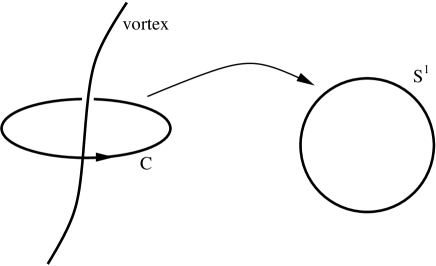
Abbildung 3.1: Mapping of the contour $C$ onto the unit circle $S^{1}$, defined by the phase of order parameter. The image of the mapping provides information about the spatial structure of the order parameter and therefore determines the topological stability of the vortex.

A vortex in a superconductor is a line along which the system is in the normal-conducting state. Typically, in a type-II superconductor, there is a special pattern of vortices along which a magnetic field can penetrate. The width of the vortices is characterized by the coherence length. Under certain conditions, this special configuration of the system corresponds to a minimum of the free energy and therefore is preferred over the completely superconducting or completely normal-conducting state. Without detailed calculations, one can use topological arguments for a prediction of the (topological) stability of the vortex. At this point, it should be mentioned that vortices are a special case of “topological defects” that may occur in any system that is characterized by a nonvanishing order parameter (i.e., superconductors, superfluids, ferromagnets, etc.). These defects can be pointlike (= monopoles), one-dimensional lines (= vortices) or surfaces (= domain walls). Let us briefly discuss the topological stability of a line defect in an ordinary superconductor. Employing the notation introduced in Sec. 1, in a conventional superconductor we have $G=U(1)$, $H=\{{\bf 1}\}$, and $G/H=U(1)$, i.e., the electromagnetic gauge group is spontaneously broken. Now consider a space-dependent order parameter

$$\psi({\bf r})=\psi_{0}\,e^{i\varphi({\bf r})}\,\,.$$ (3.5)

Mathematically, $\psi({\bf r})$ is singular along the vortex line. This vortex line is called topologically stable if there is no continuous deformation of the order parameter field $\psi({\bf r})$ that removes the singularity. What does that mean? Consider a closed contour $C$ surrounding the vortex line, cf. Fig. 3.1. On each point of this line, the order parameter (3.5) has a certain value, which is defined by its phase $\varphi({\bf r})$, since we assumed the absolute value $\psi_{0}$ to be constant. Therefore, the order parameter defines a mapping from $C$ onto the unit circle $S^{1}$, which is the topological space corresponding to the group $G/H=U(1)$. The image of this mapping is a closed contour on $S^{1}$, since the order parameter field is continuous along $C$. If this closed contour can be contracted to a single point, then there is a continuous deformation to remove the singularity. This means that the vortex is (topologically) unstable. If it cannot be contracted to a single point, the vortex is stable. This is the case if the image goes around the whole circle (once or more times). The winding number of the image is called the topological charge of the vortex. Mathematically speaking, the first homotopy group $\pi_{1}$ of the broken part of the group, $G/H$, here

$$\pi_{1}(S^{1})={\cal Z}\,\,,$$ (3.6)

classifies the vortices with respect to their topological charges. Therefore, in the case of an ordinary superconductor, topological charges of 0 (unstable), 1, 2, $\ldots$ are possible for vortices. Note that in this situation, where $G/H=U(1)$, there cannot be any point defects. The reason for that is the trivial second homotopy group, $\pi_{2}(S^{1})$, since, for the investigation of point defects, one has to consider surfaces that surround a possible monopole (in a three-dimensional system).

The relatively simple situation of an ordinary superconductor becomes more involved in the case of a more complicated group $G/H$ that possibly also allows for point or surface defects. In the case of a spin-one color superconductor, this group has a rich structure. Again, from the theory of ³He (where the group structure is similar) one could borrow the method to tackle the problem of topological defects in superfluid/superconducting quark matter, especially in spin-one color superconductors. Since they are superconductors of type I, there are no magnetic flux tubes; however, regarding superfluidity, it could be interesting to study the vortex structure.

Anhang A Projecting onto eigenspaces

In this appendix we prove Eq. (2.34) of Sec. 2.1.2.

Consider a hermitian matrix $L$ with $n$ different (real) eigenvalues $\lambda_{r}$ ($r=1,\ldots,n$). Then, the projectors $P_{r}$ onto the corresponding eigenspaces can be written as

$$P_{r}=\prod_{s\neq r}\frac{L-\lambda_{s}}{\lambda_{r}-\lambda_{s}}\,\,.$$ (A.1)

This is Eq. (2.34) in a slightly simplified notation.

Proof: $L$ can be written as

$$L=\sum_{m=1}^{n}\lambda_{m}P_{m}\,\,.$$ (A.2)

Since $L$ is hermitian, the eigenspaces are orthogonal to each other,

$$\forall r\neq s:\qquad P_{r}P_{s}=0\,\,,$$ (A.3)

and the set of projectors is complete,

$$\sum_{m=1}^{n}P_{m}={\bf 1}\,\,.$$ (A.4)

With these relations, one obtains for a fixed number $s\leq n$,

$$L-\lambda_{s}=\sum_{m=1}^{n}(\lambda_{m}-\lambda_{s})\,P_{m}\,\,.$$ (A.5)

Consequently, for a fixed number $r\leq n$,

$$\prod_{s\neq r}(L-\lambda_{s}) = \prod_{s\neq r}\sum_{m=1}^{n}(\lambda_{m}-\lambda_{s})\,P_{m}$$ (A.6)

$$= \prod_{s\neq r}(\lambda_{r}-\lambda_{s})\,P_{r}\,\,.$$ (A.7)

In this product, the only projector that survives is $P_{r}$, since this is the only one that occurs in each factor. For every other projector $P_{m}$, $m\neq r$, there is one factor that does not contain $P_{m}$, and, consequently, via Eq. (A.3), all these projectors disappear. Now, since $\lambda_{r}\neq\lambda_{s}$ for $r\neq s$, we immediately conclude for all $r\leq n$

$$P_{r}=\prod_{s\neq r}\frac{L-\lambda_{s}}{\lambda_{r}-\lambda_{s}}\,\,,$$ (A.8)

which is Eq. (A.1) and thus proves Eq. (2.34).

Anhang B Integrating over gluon momentum

In this appendix, we compute the integrals over the gluon 3-momentum $p$ to subleading order in the gap equation, leading to Eq. (2.56) in Sec. 2.1.3. We shall see that to this order it is consistent to put $k=q=\mu$.

After replacing $\hat{\mathbf{k}}\cdot\hat{\mathbf{q}}=(k^{2}+q^{2}-p^{2})/(2kq)$, the coefficients $\eta_{2m}^{\ell,t}(ee^{\prime},k,q)$ can be read off from the results of the traces ${\cal T}_{\mu\nu}^{ee^{\prime},s}({\bf k},{\bf q})$, defined in Eq. (2.48). One first observes that for all cases considered here, $\eta_{2m}^{\ell,t}(ee^{\prime},k,q)=0$ for $m\geq 3$. Next, one also realizes that $\eta_{-2}^{\ell}=0$, since there is no term in ${\cal T}_{00}^{ee^{\prime},i}$ proportional to $1/p^{2}$. Consequently, we have to compute the integrals

$${\cal I}_{2m}^{\ell}=\int_{|k-q|}^{k+q}dp\,p\,\frac{2}{p^{2}+3m_{g}^{2}}\,\left(\frac{p^{2}}{kq}\right)^{m}\,\,,\;\;\;m=0,1,2\,\,,$$ (B.1a)

for the contribution of static electric gluons to the gap equation,

$${\cal I}_{2m}^{t,1}=\int_{M}^{k+q}dp\,p\,\frac{2}{p^{2}}\,\left(\frac{p^{2}}{kq}\right)^{m}\,\,,\;\;\;m=-1,0,1,2\,\,,$$ (B.1b)

for the contribution of non-static magnetic gluons, and

$${\cal I}_{2m}^{t,2}=\int_{|k-q|}^{M}dp\,p\,\frac{p^{4}}{p^{6}+M^{4}\omega_{\pm}^{2}}\,\left(\frac{p^{2}}{kq}\right)^{m}\,\,,\;\;\;m=-1,0,1,2\,\,,$$ (B.1c)

with $\omega_{\pm}\equiv\epsilon_{q,s}^{e^{\prime}}\pm\epsilon_{k,r}^{e}$, for the contribution of almost static magnetic gluons. The result for the integrals (B.1a) and (B.1b) is

$${\cal I}_{0}^{\ell} = \ln\left[\frac{(k+q)^{2}+3m_{g}^{2}}{(k-q)^{2}+3m_{g}^{2}}\right]\simeq\ln\left(\frac{4\mu^{2}}{3m_{g}^{2}}\right)\,\,,$$ (B.2a)

$${\cal I}_{2}^{\ell} = 4-\frac{3m_{g}^{2}}{kq}\,\ln\left[\frac{(k+q)^{2}+3m_{g}^{2}}{(k-q)^{2}+3m_{g}^{2}}\right]\simeq 4\,\,,$$ (B.2b)

$${\cal I}_{4}^{\ell} = 4\,\frac{k^{2}+q^{2}-3m_{g}^{2}}{kq}+\left(\frac{3m_{g}^{2}}{kq}\right)^{2}\,\ln\left[\frac{(k+q)^{2}+3m_{g}^{2}}{(k-q)^{2}+3m_{g}^{2}}\right]\simeq 8\,\,,$$ (B.2c)

$${\cal I}_{-2}^{t,1} = \frac{kq}{M^{2}}-\frac{kq}{(k+q)^{2}}\simeq\frac{\mu^{2}}{M^{2}}-\frac{1}{4}\,\,,$$ (B.2d)

$${\cal I}_{0}^{t,1} = \ln\left[\frac{(k+q)^{2}}{M^{2}}\right]\simeq\ln\left(\frac{4\mu^{2}}{M^{2}}\right)\,\,,$$ (B.2e)

$${\cal I}_{2}^{t,1} = \frac{(k+q)^{2}-M^{2}}{kq}\simeq 4\,\,,$$ (B.2f)

$${\cal I}_{4}^{t,1} = \frac{(k+q)^{4}-M^{4}}{2(kq)^{2}}\simeq 8\,\,.$$ (B.2g)

The approximate equalities on the right-hand sides hold to subleading order in the gap equation. One obtains them employing two approximations. First, terms proportional to at least one power of $m_{g}^{2}$ or $M^{2}$ carry at least two additional powers of $g$, which renders them sub-subleading and thus negligible to the order we are computing. Second, one utilizes the fact that the $q$ integration in the gap equation is over a region of size $2\delta$ around the Fermi surface, where $\delta\sim m_{g}$. To subleading order it is thus accurate to put $k=q=\mu$ (see discussion in Sec. 2.1.3). This then yields the right-hand sides of Eqs. (B.2).

Note that there is a term $\sim\mu^{2}/M^{2}\sim 1/g^{2}$ in Eq. (B.2d). This term is parametrically the largest and could in principle give the dominant contribution to the gap equation. However, in all cases considered here, it turns out that the coefficient $\eta_{-2}^{t}$ is proportional to at least one power of $(k-q)^{2}$. Performing also the $q$ integration in the gap equation, one then has terms of the form

$$g^{2}\int_{0}^{\delta}\frac{d(q-\mu)}{\epsilon_{q}}\,\frac{(k-q)^{2}}{M^{2}}\,\phi(\epsilon_{q},q)\sim g^{2}\,\frac{\phi_{0}}{M^{2}}\int_{0}^{\delta}\frac{d\xi}{\sqrt{\xi^{2}+\phi_{0}^{2}}}\,\xi^{2}\sim g^{2}\,\phi_{0}\,\frac{\delta^{2}}{M^{2}}+O\left(\frac{\phi_{0}^{3}}{\mu^{2}}\right)\,\,,$$ (B.3)

where for the purpose of power counting we have neglected the $q$ dependence of the gap function, $\phi(\epsilon_{q},q)\sim\phi_{0}$, and we have evaluated the integral on the left-hand side for $k=\mu$. As long as $\delta\sim m_{g}\sim M$, the leading term in Eq. (B.3) is $\sim g^{2}\phi_{0}$, and thus it is only of sub-subleading order in the gap equation. It is obvious that the constant term $-1/4$ in Eq. (B.2d) is parametrically even smaller. The contribution to the term $\sim\eta_{-2}^{t}$ from non-static magnetic gluons is therefore negligible to subleading order.

Finally, also the integrals ${\cal I}_{2m}^{t,2}$ can be computed analytically [135]. Defining $\alpha\equiv(M^{4}\omega_{\pm}^{2})^{1/3}$, the result is

$${\cal I}_{-2}^{t,2} = -\frac{kq}{12\alpha}\,\left\{\ln\left[\frac{(x+\alpha)^{2}}{x^{2}-\alpha x+\alpha^{2}}\right]-2\sqrt{3}\,{\rm arctg}\,\left(\frac{2x-\alpha}{\sqrt{3}\,\alpha}\right)\right\}^{M^{2}}_{(k-q)^{2}}\,\,,$$ (B.4a)

$${\cal I}_{0}^{t,2} = \frac{1}{6}\,\ln\left[\frac{M^{6}+\alpha^{3}}{(k-q)^{6}+\alpha^{3}}\right]\simeq\frac{1}{6}\,\ln\left(\frac{M^{2}}{\omega_{\pm}^{2}}\right)\,\,,$$ (B.4b)

$${\cal I}_{2}^{t,2} = \frac{M^{2}-(k-q)^{2}}{2kq}-\frac{\alpha}{12kq}\,\left\{\ln\left[\frac{(x+\alpha)^{2}}{x^{2}-\alpha x+\alpha^{2}}\right]+2\sqrt{3}\,{\rm arctg}\,\left(\frac{2x-\alpha}{\sqrt{3}\,\alpha}\right)\right\}^{M^{2}}_{(k-q)^{2}}\simeq 0\,\,,$$ (B.4c)

$${\cal I}_{4}^{t,2} = \frac{M^{4}-(k-q)^{4}}{4(kq)^{2}}-\frac{\alpha^{3}}{(kq)^{3}}\,{\cal I}_{-2}^{t,2}\simeq 0\,\,.$$ (B.4d)

Here, we used the short notation $\{f(x)\}^{a}_{b}\equiv f(a)-f(b)$. In order to obtain the approximate equalities on the right-hand sides of Eqs. (B.4b), (B.4c), and (B.4d), one employs the fact that typically $(k-q)^{2}\sim\omega_{\pm}^{2}\ll M^{2}$, such that parametrically $(k-q)^{2}\ll\alpha\ll M^{2}$. This immediately yields the right-hand side of Eq. (B.4b). For Eqs. (B.4c) and (B.4d), we use this estimate in order to expand the logarithm occurring in Eqs. (B.4a) and (B.4c). One finds that the leading term is $\sim\alpha/M^{2}$. Similarly, one expands the inverse tangent occurring in these equations, which leads to terms which are even of order $O(1)$. Collecting all prefactors, however, all terms in Eqs. (B.4c) and (B.4d) are then suppressed by at least one power of $g^{2}$. These sub-subleading corrections are negligible to the order we are computing.

Somewhat more care is necessary in estimating the terms in Eq. (B.4a). Again, one may expand the logarithm and the inverse tangent. Together with the prefactor, this leads to a term $\sim 1/M^{2}$ for the logarithm, and a term $\sim 1/\alpha$ for the inverse tangent. The first term is harmless: together with the factor $(k-q)^{2}$ from $\eta_{-2}^{t}$ it leads to an integral of the form (B.3), which was already shown to give a sub-subleading contribution to the gap equation. The other term leads to the integral

$$g^{2}\int_{0}^{\delta}\frac{d(q-\mu)}{\epsilon_{q}}\,\frac{(k-q)^{2}}{\alpha}\,\phi(\epsilon_{q},q)\sim g^{2}\,\frac{\phi_{0}}{M^{4/3}}\int_{0}^{\delta}\frac{d\xi\,\xi^{2}}{(\xi^{2}+\phi_{0}^{2})^{5/6}}\,\,,$$ (B.5)

where we used similar power-counting arguments as in Eq. (B.3). The last integral is finite even for $\phi_{0}=0$, so that we can estimate it to be $\sim\delta^{4/3}$. For $\delta\sim m_{g}$ this contribution is then again $\sim g^{2}\phi_{0}$ and thus of sub-subleading order in the gap equation.

In conclusion, also the contribution of almost static magnetic gluons to the term $\sim\eta_{-2}^{t}$ is of sub-subleading order and can be neglected. To subleading order, it is therefore consistent to put $\eta_{-2}^{t}=0$ from the beginning, provided one chooses $\delta\sim m_{g}$.

Anhang C Computing eigenvalues

In this appendix, we compute the eigenvalues of the matrix $L_{\bf k}$, defined in Eq. (2.32), for several color-superconducting phases.

The eigenvalues $\lambda_{r}$ of $L_{\bf k}$ follow from the roots of

$${\rm det}\left(\lambda\,{\bf 1}-L_{\bf k}\right)=0\,\,.$$ (C.1)

The left-hand side of this equation can be rewritten in the form

$${\rm det}\left(\lambda\,{\bf 1}-L_{\bf k}\right)\equiv\exp\left\{{\rm Tr}\left[\ln\left(\lambda\,{\bf 1}-L_{\bf k}\right)\right]\right\}\,\,.$$ (C.2)

The logarithm of the matrix $\lambda\,{\bf 1}-L_{\bf k}$ is formally defined in terms of a power series,

$${\rm Tr}\left[\ln\left(\lambda\,{\bf 1}-L_{\bf k}\right)\right]=\ln\lambda\,{\rm Tr}\,{\bf 1}+{\rm Tr}\left[\ln\left(1-\frac{L_{\bf k}}{\lambda}\right)\right]=\ln\lambda\,{\rm Tr}\,{\bf 1}-\sum_{n=1}^{\infty}\frac{1}{n}\,\lambda^{-n}\,{\rm Tr}\,L_{\bf k}^{n}\,\,.$$ (C.3)

In order to proceed, one needs to know the trace of the $n$th power of the matrix $L_{\bf k}$. In the cases where $L_{\bf k}$ is a projector, we have $L_{\bf k}^{n}\equiv L_{\bf k}$. This is the case for instance in the 2SC phase, cf. Eq. (2.87). In this case, counting color and flavor degrees of freedom, the trace of $L_{\bf k}$ is 4. Therefore, we obtain for the 2SC phase

$${\rm det}\left(\lambda\,{\bf 1}-L_{\bf k}\right)=\lambda^{2}\,(\lambda-1)^{4}=0\,\,.$$ (C.4)

This yields the eigenvalues given in Eq. (2.88).

Next, let us discuss some less trivial cases, where $L_{\bf k}$ is no projector. First, consider the CFL phase. In this case, the calculation of $L_{\bf k}^{n}$ is slightly more involved. The first step is to notice that $L_{\bf k}^{2}=5\,L_{\bf k}-4\,{\bf 1}$. Repeated application of this relation allows to reduce an arbitrary number of powers of $L_{\bf k}$ to a single power, plus a term proportional to the unit matrix,

$$L_{\bf k}^{n}=a_{n}\,L_{\bf k}+b_{n}\,{\bf 1}\,\,.$$ (C.5)

Multiplying both sides of this equation by $L_{\bf k}$, one derives the recursion relation

$$a_{n+1}=5\,a_{n}-4\,a_{n-1}$$ (C.6)

for the coefficients $a_{n}$, and the identity

$$b_{n+1}=-4\,a_{n}$$ (C.7)

for the coefficients $b_{n}$. The recursion relation (C.6) can be solved with the Ansatz $a_{n}=p^{n}$, which yields a quadratic equation for $p$ with the solutions $p_{1}=4$ and $p_{2}=1$. The general solution of the recursion relation is then $a_{n}=\eta_{1}\,p_{1}^{n}+\eta_{2}\,p_{2}^{n}=\eta_{1}\,4^{n}+\eta_{2}$. The coefficients $\eta_{1}$ and $\eta_{2}$ can be determined from $a_{1}=1$ and $a_{2}=5$, such that

$$a_{n}=\frac{4^{n}-1}{3}\quad,\qquad b_{n}=-\frac{4^{n}-4}{3}\,\,.$$ (C.8)

In the CFL phase, ${\rm Tr}\,L_{\bf k}=12$ and ${\rm Tr}\,{\bf 1}=9$. Consequently,

$${\rm det}\left(\lambda\,{\bf 1}-L_{\bf k}\right)=(\lambda-4)\,(\lambda-1)^{8}=0\,\,,$$ (C.9)

which leads to Eq. (2.95).

Next, we compute the eigenvalues of $L_{\bf k}$ in the planar phase (the calculation for the polar phase is trivial and analogous to the 2SC phase). This can be done for arbitrary coefficients $\alpha$, $\beta$, i.e., for general linear combinations of longitudinal and transverse gaps. To this end, we first write Eq. (2.1.5) as

$$L_{\bf k}=J_{1}^{2}A_{1}+J_{2}^{2}A_{2}+\{J_{1},J_{2}\}\,B+[J_{1},J_{2}]\,Z\,\,,$$ (C.10)

where we used the abbreviations

$$A_{1/2} \equiv (\alpha^{2}-\beta^{2})\,\hat{k}_{1/2}^{2}+\beta^{2}\,\,,$$ (C.11a)

$$B \equiv (\alpha^{2}-\beta^{2})\,\hat{k}_{1}\hat{k}_{2}\,\,,$$ (C.11b)

$$Z \equiv \beta\left\{\alpha\left[\hat{k}_{2}\,\gamma_{\perp}^{1}(\hat{\mathbf{k}})-\hat{k}_{1}\,\gamma_{\perp}^{2}(\hat{\mathbf{k}})\right]-\beta\left[\gamma_{\perp}^{1}(\hat{\mathbf{k}})\,\gamma_{\perp}^{2}(\hat{\mathbf{k}})-\hat{k}_{1}\hat{k}_{2}\right]\right\}\,\,.$$ (C.11c)

The quantities $A_{1/2}$, $B$, and $Z$ are diagonal in color space. But while $A_{1/2}$ and $B$ are scalars, $Z$ is a nontrivial $4\times 4$ matrix in Dirac space. However, one easily verifies the following relation

$$Z^{2}=B^{2}-A_{1}A_{2}\,\,.$$ (C.12)

With the help of this relation and the (anti-)commutation properties of the color matrices $(J_{i})_{jk}=-i\epsilon_{ijk}$ one obtains $L_{\bf k}^{2}=(A_{1}+A_{2})\,L_{\bf k}$ and therefore

$$L_{\bf k}^{n}=(A_{1}+A_{2})^{n-1}\,L_{\bf k}\,\,.$$ (C.13)

Then, with ${\rm Tr}L_{\bf k}=8(A_{1}+A_{2})$, we have

$${\rm det}(\lambda-L_{\bf k})=\lambda^{4}[\lambda-(A_{1}+A_{2})]^{8}\,\,,$$ (C.14)

which, using the definition in Eq. (C.11a), proves Eq. (2.118).

Finally, we discuss the A phase. This case is special in the sense that $L_{\bf k}^{+}\neq L_{\bf k}^{-}$. (Remember that in Sec. 2.1 we introduced the simplified notation $L_{\bf k}\equiv L_{\bf k}^{+}$ since $L_{\bf k}^{-}$ was irrelevant in this section.) For the definition of $L_{\bf k}^{-}$ see Eq. (2.347). With the abbreviations of Eqs. (C.11) we can write

$$L_{\bf k}^{\pm}=J_{3}^{2}[(A_{1}+A_{2})\pm 2i\,Z]\,\,.$$ (C.15)

In order to derive an expression for the $n$-th power of $L_{\bf k}^{\pm}$, we notice that

$$(L_{\bf k}^{\pm})^{2}=2(A_{1}+A_{2})L_{\bf k}^{\pm}-[(A_{1}-A_{2})^{2}+4B^{2}]J_{3}^{2}\,\,,$$ (C.16)

where Eq. (C.12) has been used. Since $A_{1/2}$ and $B$ are scalars and $J_{3}^{2}L_{\bf k}^{\pm}=L_{\bf k}^{\pm}$, we have

$$(L_{\bf k}^{\pm})^{n}=a_{n}L_{\bf k}^{\pm}+b_{n}J_{3}^{2}\,\,,$$ (C.17)

with real coefficients $a_{n}$, $b_{n}$. Applying Eq. (C.16), one derives the following recursion relations for these coefficients,

$$a_{n+1}=2(A_{1}+A_{2})\,a_{n}+b_{n}\,\,,\qquad b_{n+1}=-[(A_{1}-A_{2})^{2}+4B^{2}]\,a_{n}\,\,.$$ (C.18)

With the ansatz of a power series, $a_{n}=p^{n}$, one obtains a quadratic equation for $p$, which has the two solutions

$$p_{1/2}=A_{1}+A_{2}\pm 2\sqrt{A_{1}A_{2}-B^{2}}\,\,.$$ (C.19)

Therefore, $a_{n}$ is a linear combination of the $n$-th powers of these solutions, $a_{n}=\eta_{1}\,p_{1}^{n}+\eta_{2}\,p_{2}^{n}$. The coefficients $\eta_{1}$, $\eta_{2}$ can be determined from $a_{1}=1$, $a_{2}=2(A_{1}+A_{2})$. One finds

$$a_{n}=\frac{1}{4}\frac{1}{\sqrt{A_{1}A_{2}-B^{2}}}(p_{1}^{n}-p_{2}^{n})\,\,,\qquad b_{n}=-\frac{1}{4}\frac{(A_{1}-A_{2})^{2}+4B^{2}}{\sqrt{A_{1}A_{2}-B^{2}}}(p_{1}^{n-1}-p_{2}^{n-1})\,\,.$$ (C.20)

With ${\rm Tr}L_{\bf k}^{\pm}=8(A_{1}+A_{2})$ this yields

$${\rm det}(\lambda-L_{\bf k}^{\pm})=\lambda^{4}(\lambda-p_{1})^{4}(\lambda-p_{2})^{4}\,\,.$$ (C.21)

Consequently, both $L_{\bf k}^{+}$ and $L_{\bf k}^{-}$ have the eigenvalues 0, $p_{1}$, and $p_{2}$, each with degeneracy 4, which proves Eqs. (2.1.5).

Finally, consider the projectors ${\cal P}_{{\bf k},r}^{\pm}$ corresponding to the eigenvalues $\lambda$ (in Sec. 2.1, ${\cal P}_{\bf k}^{r}\equiv{\cal P}_{{\bf k},r}^{+}$). With Eq. (2.34),

$${\cal P}_{{\bf k},1/2}^{\pm}=\frac{L_{\bf k}^{\pm}(L_{\bf k}^{\pm}-\lambda_{2/1})}{\lambda_{1/2}(\lambda_{1/2}-\lambda_{2/1})}\,\,,\qquad{\cal P}_{{\bf k},3}^{\pm}={\bf 1}-{\cal P}_{{\bf k},1}^{\pm}-{\cal P}_{{\bf k},2}^{\pm}\,\,.$$ (C.22)

This leads to

$${\cal P}_{{\bf k},1}^{\pm} = \frac{1}{2}J_{3}^{2}\left(1\pm\frac{i}{\sqrt{A_{1}A_{2}-B^{2}}}\,Z\right)\,\,,$$ (C.23a)

$${\cal P}_{{\bf k},2}^{\pm} = \frac{1}{2}J_{3}^{2}\left(1\mp\frac{i}{\sqrt{A_{1}A_{2}-B^{2}}}\,Z\right)\,\,,$$ (C.23b)

$${\cal P}_{{\bf k},3}^{\pm} = 1-J_{3}^{2}\,\,.$$ (C.23c)

Since ${\rm Tr}Z={\rm Tr}(\Lambda_{\bf k}^{e}Z)=0$, one immediately proves Eq. (2.357). Note that, making use of Eq. (C.12), Eqs. (C.23a) and (C.23b) can be written as

$${\cal P}_{{\bf k},1}^{\pm} = \frac{1}{2}J_{3}^{2}\left(1\pm\frac{Z}{\sqrt{Z^{2}}}\right)\,\,,$$ (C.24a)

$${\cal P}_{{\bf k},2}^{\pm} = \frac{1}{2}J_{3}^{2}\left(1\mp\frac{Z}{\sqrt{Z^{2}}}\right)\,\,.$$ (C.24b)

Anhang D Proving $d=6$ for longitudinal gaps

In this appendix, we prove that $d=6$ for any order parameter (= for any $3\times 3$ matrix) $\Delta$ in the case of a longitudinal gap. The constant $d$ occurs in the value of the gap at the Fermi surface for $T=0$, cf. Eq. (2.41), and is defined in Eq. (2.59). The longitudinal case, i.e., $(\alpha,\beta)=(1,0)$ in Eq. (2.99) is particularly simple, since in this case the Dirac structure of the matrix ${\cal M}_{\bf k}$ is trivial.

In order to compute the constant $d$, we use the method presented in Sec. 2.1.3. We have to determine the eigenvalues of $L_{\bf k}$ in order to compute the quantities ${\cal T}_{00}^{ee^{\prime},s}({\bf k},{\bf q})$ and ${\cal T}_{t}^{ee^{\prime},s}({\bf k},{\bf q})$.

Let us start with the matrix

$${\cal M}_{\bf k}=\mbox{\boldmath${v}$}_{\bf k}\cdot\mbox{\boldmath${J}$}\,\,,$$ (D.1)

where we abbreviated $\mbox{\boldmath${v}$}_{\bf k}=(v_{{\bf k},1},v_{{\bf k},2},v_{{\bf k},3})$ with

$$v_{{\bf k},i}\equiv\sum_{j=1}^{3}\Delta_{ij}\hat{k}_{j}\,\,,\qquad i=1,2,3\,\,.$$ (D.2)

Then,

$$(L_{\bf k})_{ij}=v_{\bf k}^{2}\,\delta_{ij}-v^{*}_{{\bf k},j}\,v_{{\bf k},i}\,\,,$$ (D.3)

where $v_{\bf k}^{2}\equiv\mbox{\boldmath${v}$}_{\bf k}^{*}\cdot\mbox{\boldmath${v}$}_{\bf k}$. Now, with $L_{\bf k}^{2}=v_{\bf k}^{2}\,L_{\bf k}$ and ${\rm Tr}\,L_{\bf k}=8\,v^{2}_{\bf k}$ the eigenvalues of $L_{\bf k}$ are easily found making use of the method presented in Appendix C. One obtains

$$\lambda_{1}=v_{\bf k}^{2}\qquad(\mbox{8-fold})\,\,,\qquad\lambda_{2}=0\qquad(\mbox{4-fold})\,\,.$$ (D.4)

Consequently, the fact that there is one gapped branch with degeneracy 8 and one ungapped branch with degeneracy 4 is completely general, i.e., it is true for any order parameter $\Delta$ in the longitudinal case. The corresponding projectors are given by

$$({\cal P}_{\bf k}^{1})_{ij}=\delta_{ij}-\frac{v_{{\bf k},i}^{*}v_{{\bf k},j}}{v^{2}}\,\,,\qquad({\cal P}_{\bf k}^{2})_{ij}=\frac{v_{{\bf k},i}^{*}v_{{\bf k},j}}{v^{2}}\,\,.$$ (D.5)

Using Eqs. (2.48) and (2.50), this leads to

$${\cal T}_{00}^{ee^{\prime},1}({\bf k},{\bf q}) = \frac{1}{3}\,\frac{\mbox{\boldmath${v}$}_{\bf q}\cdot\mbox{\boldmath${v}$}_{\bf k}^{*}}{v_{\bf k}^{2}}\,(1+ee^{\prime}\hat{\mathbf{q}}\cdot\hat{\mathbf{k}})\,\,,$$ (D.6a)

$${\cal T}_{t}^{ee^{\prime},1}({\bf k},{\bf q}) = \frac{2}{3}\,\frac{\mbox{\boldmath${v}$}_{\bf q}\cdot\mbox{\boldmath${v}$}_{\bf k}^{*}}{v_{\bf k}^{2}}\,(1-ee^{\prime}\hat{\mathbf{p}}\cdot\hat{\mathbf{q}}\,\hat{\mathbf{p}}\cdot\hat{\mathbf{k}})\,\,,$$ (D.6b)

and ${\cal T}_{\mu\nu}^{ee^{\prime},2}({\bf k},{\bf q})=0$. In order to perform the angular integration, we choose a coordinate system $(q,\theta^{\prime},\varphi^{\prime})$, such that $\hat{\mathbf{q}}\cdot\hat{\mathbf{k}}=\cos\theta^{\prime}$. With ${\bf k}=k\,(\sin\theta\cos\varphi,\sin\theta\sin\varphi,\cos\theta)$, this is achieved by a rotation

$$R(\theta,\varphi)=\left(\begin{array}[]{ccc}\cos\theta\,\cos\varphi&\cos\theta\,\sin\varphi&-\sin\theta\\ -\sin\varphi&\cos\varphi&0\\ \sin\theta\,\cos\varphi&\sin\theta\,\sin\varphi&\cos\theta\end{array}\right)\,\,,$$ (D.7)

that rotates the original coordinate system into a new one whose $z^{\prime}$-axis is parallel to $\hat{\mathbf{k}}$. Consequently, ${\bf q}$ has to be written as ${\bf q}=R^{-1}(\theta,\varphi)\,{\bf q}^{\prime}$ with ${\bf q}^{\prime}=q\,(\sin\theta^{\prime}\cos\varphi^{\prime},\sin\theta^{\prime}\sin\varphi^{\prime},\cos\theta^{\prime})$. After this transformation and the integration over $\varphi^{\prime}$ one obtains (note that there is neither a $\theta$- nor a $\varphi$-dependence left)

$$\frac{1}{2\pi}\int_{0}^{2\pi}d\varphi^{\prime}\,{\cal T}_{00}^{ee^{\prime},s}({\bf k},{\bf q}) = \frac{1}{3}\,\hat{\mathbf{q}}\cdot\hat{\mathbf{k}}\,(1+ee^{\prime}\,\hat{\mathbf{q}}\cdot\hat{\mathbf{k}})\,\,,$$ (D.8a)

$$\frac{1}{2\pi}\int_{0}^{2\pi}d\varphi^{\prime}\,{\cal T}_{t}^{ee^{\prime},s}({\bf k},{\bf q}) = \frac{2}{3}\,\hat{\mathbf{q}}\cdot\hat{\mathbf{k}}\,(1-ee^{\prime}\,\hat{\mathbf{p}}\cdot\hat{\mathbf{q}}\,\hat{\mathbf{p}}\cdot\hat{\mathbf{k}})\,\,.$$ (D.8b)

The $\theta^{\prime}$-integration is performed in terms of an integral over $p$, cf. Sec. 2.1.3 and Appendix B. The result of this integration is taken care of by Eq. (2.59). We may set $e=e^{\prime}$ which is equivalent to neglecting the antiparticle gap. Finally, via ${\bf p}={\bf k}-{\bf q}$ we find

$$\eta_{0}^{\ell}=\frac{2}{3}\quad,\qquad\eta_{2}^{\ell}=-\frac{1}{2}\quad,\qquad\eta_{4}^{\ell}=\frac{1}{12}\quad,\qquad\eta_{0}^{t}=\frac{2}{3}\quad,\qquad\eta_{2}^{t}=-\frac{1}{6}\quad,\qquad\eta_{4}^{t}=-\frac{1}{12}\,\,.$$ (D.9)

With Eq. (2.59), this proves the result $d=6$.

Anhang E Integrating over quark momentum

In this appendix, we prove the results shown in Table 2.4, i.e., we calculate the integrals over quark momentum defined in Eqs. (2.279). In this calculation we neglect the antiparticle gap, $\phi^{-}\simeq 0$.

Contributions from normal propagators at $T=0$

We start from Eqs. (2.270) which, for $p_{0}=0$ reduce to (cf. Eq. (2.272))

$$v_{e_{1}e_{2}}^{rs}=-\frac{\epsilon_{1,r}\epsilon_{2,s}-\xi_{1}\xi_{2}}{2\epsilon_{1,r}\epsilon_{2,s}(\epsilon_{1,r}+\epsilon_{2,s})}(1-N_{1,r}-N_{2,s})+\frac{\epsilon_{1,r}\epsilon_{2,s}+\xi_{1}\xi_{2}}{2\epsilon_{1,r}\epsilon_{2,s}(\epsilon_{1,r}-\epsilon_{2,s})}(N_{1,r}-N_{2,s})\,\,.$$ (E.1)

Here, we inserted the definition of $n_{i,r}$ given in Eq. (2.271) and defined

$$\xi_{i}\equiv e_{i}k_{i}-\mu\,\,.$$ (E.2)

In the limit $p\to 0$, or, equivalently, $k_{1}\to k_{2}$, we obtain for $r=1,2$

$$v^{rr}\simeq-\frac{1}{\mu^{2}}\int_{0}^{\infty}dk\,k^{2}\left[\frac{\lambda_{r}\phi^{2}}{4\epsilon_{r}^{3}}(1-2N_{r})-\frac{\epsilon_{r}^{2}+\xi^{2}}{2\epsilon_{r}^{2}}\frac{dN_{r}}{d\epsilon_{r}}\right]\,\,,$$ (E.3)

where we used $(N_{1,r}-N_{2,r})/(\epsilon_{1,r}-\epsilon_{2,r})\simeq dN_{r}/d\epsilon_{r}$ and $\xi\equiv k-\mu$. All quantities now depend on $k_{1}=k$ and correspond to positive energies, $e_{1}=e_{2}=1$, since, due to $\phi^{-}\simeq 0$, the terms corresponding to negative energies vanish. Therefore, we omit the index $i=1,2$. Note that, up to subleading order, the gap function does not depend on the index $r$, $\phi_{1}\simeq\phi_{2}\equiv\phi$ [98]. We have to distinguish between the cases where $\lambda_{r}\neq 0$ and where $\lambda_{r}=0$. When $\lambda_{r}\neq 0$, we obtain for zero temperature $T=0$, where $N_{r}=0$,

$$v^{rr}=-\frac{1}{\mu^{2}}\int_{0}^{\infty}dk\,k^{2}\frac{\lambda_{r}\phi^{2}}{4\epsilon_{r}^{3}}\simeq-\frac{1}{2}\int_{0}^{\mu}d\xi\lambda_{r}\phi^{2}(\xi^{2}+\lambda_{r}\phi^{2})^{-3/2}\simeq-\frac{1}{2}\,\,.$$ (E.4)

Here, we restricted the $k$-integration to the region $0\leq k\leq 2\mu$ since the gap function is strongly peaked around the Fermi surface, $k=\mu$. In this region, we assume that the gap function does not depend on the momentum $k$. Since the eigenvalue $\lambda_{r}$ cancels out, this result does not depend on $r$. Therefore, it gives rise to the value of $v^{11}$ for all four considered phases and for $v^{22}$ in the cases of the CFL and CSL phases. When $\lambda_{r}=0$, we obtain (for arbitrary temperature $T$)

$$v^{rr}=\frac{1}{\mu^{2}}\int_{0}^{\infty}dk\,k^{2}\frac{dN_{F}}{dk}\,\,,$$ (E.5)

where $N_{F}\equiv 1/[\exp(\xi/T)+1]$ is the Fermi distribution. Using $\mu\gg T$, and the substitution $\zeta=\xi/2T$, this can be transformed to

$$v^{rr}\simeq-\int_{0}^{\infty}d\zeta\frac{1}{\cosh^{2}\zeta}=-1\,\,.$$ (E.6)

Let us now compute $v^{rs}$ for $r\neq s$. Using Eq. (E.1), we obtain for two nonvanishing eigenvalues $\lambda_{1},\lambda_{2}$ and at zero temperature

$$v^{12}=v^{21}=-\frac{1}{\mu^{2}}\int_{0}^{\infty}dk\,k^{2}\frac{\epsilon_{1}\epsilon_{2}-\xi^{2}}{2\epsilon_{1}\epsilon_{2}(\epsilon_{1}+\epsilon_{2})}\simeq-\int_{0}^{\mu}d\xi\frac{1}{(\lambda_{2}-\lambda_{1})\phi^{2}}\left(\frac{\epsilon_{2}^{2}+\xi^{2}}{\epsilon_{2}}-\frac{\epsilon_{1}^{2}+\xi^{2}}{\epsilon_{1}}\right)\simeq-\frac{1}{2}\,\,.$$ (E.7)

Again, we neglected the integral over the region $k>2\mu$. In the last integral, the leading order contributions cancel. The subleading terms give rise to $(\lambda_{2}-\lambda_{1})\phi^{2}/2$. Therefore, the eigenvalues cancel and the result does not depend on $\lambda_{1},\lambda_{2}\neq 0$. Eq. (E.7) holds for the CFL and CSL phases.

When one of the excitation branches is ungapped (2SC and polar phase), for instance, $\lambda_{2}=0$, we have

$$v^{12}=v^{21}=-\frac{1}{\mu^{2}}\int_{0}^{\infty}dk\,k^{2}\left[\frac{n_{1}}{\epsilon_{1}+\xi}(1-N_{1}-N_{F})-\frac{1-n_{1}}{\epsilon_{1}-\xi}(N_{1}-N_{F})\right]\,\,.$$ (E.8)

For $T=0$, this becomes with the standard approximations

$$v^{12} \simeq -\frac{1}{\mu^{2}}\int_{-\mu}^{\mu}d\xi\frac{(\xi+\mu)^{2}}{2\epsilon_{1}}\left[\frac{\epsilon_{1}-\xi}{\epsilon_{1}+\xi}\Theta(\xi)+\frac{\epsilon_{1}+\xi}{\epsilon_{1}-\xi}\Theta(-\xi)\right]$$ (E.9)

$$= -\int_{0}^{\mu}\frac{d\xi}{\epsilon_{1}}\left(1+\frac{\xi^{2}}{\mu^{2}}\right)\frac{\epsilon_{1}-\xi}{\epsilon_{1}+\xi}\simeq-\frac{1}{2}\,\,,$$

where the last integral has already been computed in Ref. [102].

Next, we compute $\bar{v}^{rs}$ for the various cases. Setting the thermal distribution function for antiparticles to zero, we obtain with the definition in Eq. (2.279)

$$\bar{v}^{rs}=-\frac{1}{\mu^{2}}\int_{0}^{\infty}dk\,k^{2}\left[\frac{(1-n_{r})(1-N_{r})}{\epsilon_{r}^{+}+\epsilon_{s}^{-}}-\frac{N_{r}n_{r}}{\epsilon_{r}^{+}-\epsilon_{s}^{-}}+\frac{(1-n_{s})(1-N_{s})}{\epsilon_{r}^{-}+\epsilon_{s}^{+}}-\frac{N_{s}n_{s}}{\epsilon_{s}^{+}-\epsilon_{r}^{-}}\right]$$ (E.10)

with $\epsilon_{r}^{\pm}\equiv\epsilon_{k,r}^{\pm}$. Again, we first consider the situation where $r=s$. In this case, for $T=0$ and $\lambda_{r}\neq 0$, (defining $\epsilon\equiv\epsilon^{+}$)

$$\bar{v}^{rr} = -\frac{2}{\mu^{2}}\int_{0}^{\infty}dk\,k^{2}\left[\frac{1-n_{r}}{\epsilon_{r}+k+\mu}-\frac{1}{2k}\right]$$ (E.11)

$$=\frac{1}{\mu^{2}}\int_{0}^{\infty}dk\,k\,\frac{\mu(\epsilon_{r}+\mu-k)+\lambda_{r}\phi^{2}}{\epsilon_{r}(\epsilon_{r}+k+\mu)}\simeq\frac{1}{2}\,\,.$$

Here, $-1/(2k)$ is a vacuum subtraction. The last integral has been computed in Ref. [102]. Note that the result does not depend on the value of $\lambda_{r}\neq 0$. Thus, it is valid for $\bar{v}^{11}$ in the 2SC and polar phases as well as for both $\bar{v}^{11}$ and $\bar{v}^{22}$ in the CFL and CSL phases.

For $\lambda_{r}=0$, we obtain from Eq. (E.10) at zero temperature and with the vacuum subtraction $1/(2k)$

$$\bar{v}^{rr}=-\frac{2}{\mu^{2}}\int_{0}^{\infty}dk\,k^{2}\left[\frac{\Theta(k-\mu)}{2k}-\frac{1}{2k}\right]=\frac{1}{2}\,\,.$$ (E.12)

This result holds for $\bar{v}^{22}$ in the 2SC and polar phases.

Next, we discuss the case $r\neq s$. From Eqs. (E.10) and (E.11) it is obvious that, since the result for $\bar{v}^{rr}$ did not depend on $\lambda_{r}$, we get the same result for $\bar{v}^{rs}$ with two nonvanishing eigenvalues $\lambda_{1},\lambda_{2}\neq 0$. Thus, in this case,

$$\bar{v}^{12}=\bar{v}^{21}=\frac{1}{2}\,\,.$$ (E.13)

For $\lambda_{2}=0$, we obtain at zero temperature

$$\bar{v}^{12}=\bar{v}^{21}=-\frac{1}{\mu^{2}}\int_{0}^{\infty}dk\,k^{2}\left[\frac{1-n_{1}}{\epsilon_{1}+k+\mu}+\frac{\Theta(k-\mu)}{2k}-\frac{3}{2k}\right]\simeq\frac{1}{2}\,\,,$$ (E.14)

where identical integrals as in Eqs. (E.11) and (E.12) were performed. Consequently, also for the 2SC and polar phases, Eq. (E.13) holds.

Contributions from anomalous propagators at $T=0$

We start from Eq. (2.274) which, for $p_{0}=0$, is

$$w_{e_{1}e_{2}}^{rs}=\frac{\phi^{e_{1}}\phi^{e_{2}}}{2\epsilon_{1,r}\epsilon_{2,s}(\epsilon_{1,r}+\epsilon_{2,s})}(1-N_{1,r}-N_{2,s})+\frac{\phi^{e_{1}}\phi^{e_{2}}}{2\epsilon_{1,r}\epsilon_{2,s}(\epsilon_{1,r}-\epsilon_{2,s})}(N_{1,r}-N_{2,s})\,\,.$$ (E.15)

Obviously, since $\phi^{-}\simeq 0$, for all $r$, $s$ and all phases we have $\bar{w}^{rs}=0$ (for the definition of $\bar{w}^{rs}$ cf. Eq. (2.279)). First, we calculate $w^{rs}$ for $r=s$. Neglecting the antiparticle gap and taking the limit $k_{1}\to k_{2}$, we obtain, using the same notation as above, $\epsilon_{r}\equiv\epsilon^{+}_{k,r}$,

$$w^{rr}=\frac{1}{\mu^{2}}\int_{0}^{\infty}dk\,k^{2}\left[\frac{\phi^{2}}{4\epsilon_{r}^{3}}(1-2N_{r})+\frac{\phi^{2}}{2\epsilon_{r}^{2}}\frac{dN_{r}}{d\epsilon_{r}}\right]\,\,.$$ (E.16)

For $\lambda_{r}\neq 0$ and at zero temperature, where $N_{r}=0$, this expression reduces to

$$w^{rr}=\frac{1}{\mu^{2}}\int_{0}^{\infty}dk\,k^{2}\frac{\phi^{2}}{4\epsilon_{r}^{3}}\simeq\frac{1}{2}\int_{0}^{\mu}\delta\xi\,\phi^{2}(\xi^{2}+\lambda_{r}\phi^{2})^{-3/2}\simeq\frac{1}{2\lambda_{r}}\,\,.$$ (E.17)

Unlike in $v^{rr}$, the eigenvalue $\lambda_{r}$ does not cancel out and we obtain different results for $\lambda_{r}=4$ and $\lambda_{r}=1$. (Remember the different normalization compared to Sec. 2.1, cf. Eqs. (2.281) and comments above these equations.) In the cases of the 2SC and polar phases we obtain $w^{11}=1/2$ whereas for the CFL and CSL phases, $w^{11}=1/8$ and $w^{22}=1/2$. In the former two cases, the quantity $w^{22}$ does not occur in our calculation. Thus we can turn to the case where $r\neq s$. Here, we conclude from Eq. (E.15)

$$w^{12}=w^{21}=\frac{1}{\mu^{2}}\int_{0}^{\infty}dk\,k^{2}\left[\frac{\phi^{2}}{2\epsilon_{1}\epsilon_{2}(\epsilon_{1}+\epsilon_{2})}(1-N_{1}-N_{2})+\frac{\phi^{2}}{2\epsilon_{1}\epsilon_{2}(\epsilon_{1}-\epsilon_{2})}(N_{1}-N_{2})\right]\,\,.$$ (E.18)

For two nonvanishing eigenvalues $\lambda_{1}$, $\lambda_{2}$, this reads at $T=0$

$$w^{12} = \frac{1}{\mu^{2}}\int_{0}^{\infty}dk\,k^{2}\frac{\phi^{2}}{2\epsilon_{1}\epsilon_{2}(\epsilon_{1}+\epsilon_{2})}\simeq\frac{1}{\lambda_{1}-\lambda_{2}}\int_{0}^{\mu}d\xi\,\left(\frac{1}{\epsilon_{2}}-\frac{1}{\epsilon_{1}}\right)$$ (E.19)

$$\simeq \frac{1}{2}\frac{1}{\lambda_{1}-\lambda_{2}}\ln\frac{\lambda_{1}}{\lambda_{2}}\,\,.$$

For $\lambda_{1}=4$ and $\lambda_{2}=1$ (CFL and CSL phases) we obtain

$$w^{12}=w^{21}=\frac{1}{3}\ln 2\,\,.$$ (E.20)

The corresponding expression for the case where the second eigenvalue vanishes, $\lambda_{2}=0$, does not occur in our calculation.

Integrals in the normal phase, $T\geq T_{c}$

For temperatures larger than the transition temperature $T_{c}$ but still much smaller than the chemical potential, $T\ll\mu$, all integrals defined in Eqs. (2.279) are easily computed. Since there is no gap in this case, $\phi=0$, all contributions from the anomalous propagators vanish trivially, $w^{rs}=\bar{w}^{rs}=0$. From Eq. (E.1), which holds for all temperatures, we find with $\phi=0$

$$v^{11}=v^{22}=v^{12}=\frac{1}{\mu^{2}}\int_{0}^{\infty}dk\,k^{2}\frac{dN_{F}}{d\xi}\simeq-1$$ (E.21)

and (with the vacuum subtraction $1/k$)

$$\bar{v}^{11}=\bar{v}^{22}=\bar{v}^{12}=-\frac{1}{\mu^{2}}\int_{0}^{\infty}dk\,k^{2}\left[\frac{1-N_{F}}{k}-\frac{1}{k}\right]\simeq\frac{1}{2}\,\,.$$ (E.22)

Anhang F Summing over Matsubara frequencies

In this appendix, we prove Eqs. (2.352) and (2.355). For further details concerning Matsubara frequencies see for instance Refs. [121, 136].

In order to prove Eq. (2.352), we compute $\sum_{k_{0}}(\epsilon_{k}^{2}-k_{0}^{2})/T^{2}$ via performing the sum over fermionic Matsubara frequencies, $k_{0}=-i\omega_{n}=-i(2n+1)\pi T$. This calculation can be divided into four steps:

1. Rewrite the logarithm as an integral:

   $$\ln\frac{\epsilon_{k}^{2}-k_{0}^{2}}{T^{2}}=\int_{1}^{(\epsilon_{k}/T)^{2}}dx^{2}\,\frac{1}{x^{2}+(2n+1)^{2}\pi^{2}}+\ln[1+(2n+1)^{2}\pi^{2}]\,\,.$$ (F.1)

2. Write the sum over $k_{0}$ as a contour integral:

   Let us define the integral kernel in Eq. (F.1) as a function of $k_{0}$,

   $$f(k_{0})\equiv\frac{1}{x^{2}+(2n+1)^{2}\pi^{2}}=\frac{T^{2}}{T^{2}x^{2}-k_{0}^{2}}\,\,.$$ (F.2)

   Then, the sum over this function can be written as

   $$T\sum_{n}\left.f(k_{0})\right|_{k_{0}=-i\omega_{n}}=\frac{1}{2\pi i}\oint\limits_{C}dk_{0}\,f(k_{0})\frac{1}{2}\,\tanh\frac{k_{0}}{2T}\,\,,$$ (F.3)

   where $C$ is a contour that encloses a region in the complex plane in which all poles of $\tanh\frac{k_{0}}{2T}$ are located and where $f(k_{0})$ is analytical.

   Proof of Eq. (F.3): Remember the residue theorem

   $$\frac{1}{2\pi i}\oint\limits_{C}dz\,f(z)=\sum_{n}{\rm Res}\,\left.f(z)\right|_{z=z_{n}}\,\,,$$ (F.4)

   where $z_{n}$ are the singularities of $f$ in the area surrounded by $C$. If $f$ can be written in the form

   $$f(z)=\frac{\varphi(z)}{\psi(z)}\,\,,$$ (F.5)

   then

   $${\rm Res}\,\left.f(z)\right|_{z=z_{n}}=\frac{\varphi(z_{n})}{\psi^{\prime}(z_{n})}\,\,,$$ (F.6)

   where $z_{n}$ are the roots of $\psi(z)$ and $\psi^{\prime}\equiv d\psi/dz$. We apply this form of the residue theorem to our calculation. Since

   $$\tanh\frac{k_{0}}{2T}=\frac{e^{k_{0}/(2T)}-e^{-k_{0}/(2T)}}{e^{k_{0}/(2T)}+e^{-k_{0}/(2T)}}\,\,,$$ (F.7)

   the poles of $\frac{1}{2}f(k_{0})\tanh\frac{k_{0}}{2T}$ are given by

   $$k_{0}=-i(2n+1)\,\pi\,T=-i\omega_{n}\,\,,\qquad n\in{\cal Z}\,\,.$$ (F.8)

   With

   $$\frac{d}{dk_{0}}\left[e^{k_{0}/(2T)}+e^{-k_{0}/(2T)}\right]_{k_{0}=-i\omega_{n}}=\frac{i}{T}(-1)^{n+1}\,\,,$$ (F.9)

   and

   $$\left[e^{k_{0}/(2T)}-e^{-k_{0}/(2T)}\right]_{k_{0}=-i\omega_{n}}=2i\,(-1)^{n+1}\,\,,$$ (F.10)

   we obtain for all $n$,

   $${\rm Res}\left[f(k_{0})\frac{1}{2}\tanh\frac{k_{0}}{2T}\right]_{k_{0}=-i\omega_{n}}=T\,f(-i\omega_{n})\,\,,$$ (F.11)

   which proves Eq. (F.3).

3. Compute the contour integral:

   Since the poles of $\frac{1}{2}f(k_{0})\tanh\frac{k_{0}}{2T}$ are on the imaginary axis, we choose the contour for the integral on the right-hand side of Eq. (F.3) in the following way:

   $$\frac{1}{2\pi i}\oint\limits_{C}dk_{0}\,f(k_{0})\frac{1}{2}\,\tanh\frac{k_{0}}{2T} = \frac{1}{2\pi i}\int\limits_{-i\infty+\eta}^{i\infty+\eta}dk_{0}\,f(k_{0})\frac{1}{2}\,\tanh\frac{k_{0}}{2T}+\frac{1}{2\pi i}\int\limits_{i\infty-\eta}^{-i\infty-\eta}dk_{0}\,f(k_{0})\frac{1}{2}\,\tanh\frac{k_{0}}{2T}$$ (F.12)

   $$= \frac{1}{2\pi i}\int\limits_{-i\infty+\eta}^{i\infty+\eta}dk_{0}\,\frac{1}{2}[f(k_{0})+f(-k_{0})]\,\tanh\frac{k_{0}}{2T}$$

   $$= \frac{1}{2\pi i}\int\limits_{-i\infty+\eta}^{i\infty+\eta}dk_{0}\,\frac{T^{2}}{T^{2}x^{2}-k_{0}^{2}}\,\left(1-\frac{2}{e^{k_{0}/T}+1}\right)$$

   $$= \frac{T}{x}\left(\frac{1}{2}-\frac{1}{e^{x}+1}\right)\,\,,$$

   where, in the last step, we closed the integration path in clockwise direction (minus sign!) such that one of the poles, namely $k_{0}=Tx$ is enclosed, and used once more the residue theorem.

4. Collect the results:

   With Eqs. (F.1), (F.3), and (F.12), we now compute the Matsubara sum. Omitting the terms which do not depend on $k$, we obtain

   $$\sum_{k_{0}}\ln\frac{\epsilon_{k}^{2}-k_{0}^{2}}{T^{2}} = \int_{1}^{(\epsilon_{k}/T)^{2}}dx^{2}\,\frac{1}{x}\left(\frac{1}{2}-\frac{1}{e^{x}+1}\right)$$ (F.13)

   $$= \frac{\epsilon_{k}}{T}+2\ln\left[1+\exp\left(-\frac{\epsilon_{k}}{T}\right)\right]\,\,.$$

   This is Eq. (2.352).

Applying the same method, it is easy to prove also Eq. (2.355). With the definition

$$f(k_{0})\equiv\frac{\varphi(k_{0})}{k_{0}^{2}-\epsilon_{k}^{2}}$$ (F.14)

we can proceed along the same lines as described in 2. and 3. above. Using $\varphi(k_{0})=\varphi(-k_{0})$, we obtain

$$\sum_{k_{0}}f(k_{0}) = \frac{1}{2\pi i}\int\limits_{-i\infty+\eta}^{i\infty+\eta}dk_{0}\,f(k_{0})\,\tanh\frac{k_{0}}{2T}$$ (F.15)

$$= -\frac{\varphi(\epsilon_{k})}{2\epsilon_{k}}\,\tanh\frac{\epsilon_{k}}{2T}\,\,.$$

This is Eq. (2.355).

- [1] D.J. Gross and F. Wilczek, Phys. Rev. Lett. 30, 1343 (1973); H.D. Politzer, ibid. 1346.
- [2] J.C. Collins and M.J. Perry, Phys. Rev. Lett. 34, 1353 (1975).
- [3] see, for instance: Proc. of the 15th Int. Conf. on Ultra-relativistic Nucleus-Nucleus Collisions, Quark Matter 2001 (eds. T.J Hallmann, D.E. Kharzeev, J.T. Mitchell, and T.S. Ullrich), Nucl. Phys. A698, 1 (2002).
- [4] see, for instance: M. Creutz, Quarks, gluons and lattices (Cambridge University Press, Cambridge, 1983).
- [5] K. Wilson, Phys. Rev. D 10, 2445 (1974).
- [6] R.D. Pisarski, Phys. Rev. D 62, 111501 (2000); A. Dumitru and R.D. Pisarski, Phys. Lett. B 504, 282 (2001), Phys. Lett. B 525, 95 (2002), Phys. Rev. D 66, 096003 (2002).
- [7] E. Laermann and O. Philipsen, hep-ph/0303042.
- [8] A.C. Phillips, The Physics of Stars (John Wiley & Sons, Chichester, 1994).
- [9] F. Weber, Pulsars as Astrophysical Laboratories for Nuclear and Particle Physics (IOP Publishing Ltd., Bristol, 1999).
- [10] M. Ruderman, T. Zhu, and K. Chen, Astrophys. J. 492, 267 (1998).
- [11] J.A. Pons, S. Reddy, M. Prakash, J.M. Lattimer, and J.A. Miralles, Astrophys. J. 513, 780 (1999).
- [12] M. Prakash, J.M. Lattimer, J.A. Pons, A.W. Steiner, and S. Reddy, Lect. Notes Phys. 578, 364 (2001).
- [13] A.A. Svidzinsky, Astrophys. J. 590, 386 (2003).
- [14] A. Hewish, S.G. Bell, J.D.H. Pilkington, P.F. Scott, and R.A. Collins, Nature 217, 709 (1968); F. Pacini, Nature 219, 145 (1968); T. Gold, Nature 218, 731 (1968).
- [15] D.M. Sedrakian, A.D. Sedrakian, and G.F. Zharkov, Mon. Not. Roy. Astron. Soc. 290, 203 (1997).
- [16] B. Link, Phys. Rev. Lett. 91, 101101 (2003).
- [17] K.B.W. Buckley, M.A. Metlitski, and A.R. Zhitnitsky, Phys. Rev. Lett. 92, 151102 (2004).
- [18] X.L. Zhang, R.-X. Xu, and S.N. Zhang, astro-ph/0310049, Proc. of IAU Symposium 218: Young Neutron Stars and Their Environment, Sydney, Australia, 14-17 Jul 2003; J.E. Trümper, V. Burwitz, F. Haberl, and V.E. Zavlin, astro-ph/0312600, Proc. of Symposium on the Restless High-Energy Universe, Amsterdam, the Netherlands, 5-8 May 2003; K. Kohri, K. Sato, and K. Iida, Prog. Theor. Phys. Suppl. 151, 181 (2003).
- [19] Z.M. Galasiewicz, Superconductivity and quantum fluids (Pergamon Press, Oxford, 1970).
- [20] A.L. Fetter and J.D. Walecka, Quantum Theory of Many-Particle Systems (McGraw-Hill, New York, 1971).
- [21] M. Tinkham, Introduction to Superconductivity (McGraw-Hill, New York, 1975).
- [22] D. Vollhardt and P. Wölfle, The Superfluid Phases of Helium 3 (Taylor & Francis, London, 1990).
- [23] H. Kamerlingh Onnes, Comm. Leiden 120b (1911).
- [24] J. Bardeen, L.N. Cooper, and J.R. Schrieffer, Phys. Rev. 108, 1175 (1957).
- [25] J.G. Bednorz and K.A. Müller, Z. Physik B64, 189 (1986).
- [26] H. Fröhlich, Phys. Rev. 79, 845 (1950).
- [27] M. Sigrist and K. Ueda, Rev. Mod. Phys. 63, 239 (1991); K. Deguchi, Z.Q. Mao, H. Yaguchi, and Y. Maeno, Phys. Rev. Lett. 92, 047002 (2004).
- [28] A.P Mackenzie and Y. Maeno, Rev. Mod. Phys. 75, 657 (2003).
- [29] P. Nozières and S. Schmitt-Rink, J. Low Temp. Phys. 59, 195 (1985).
- [30] E. Babaev, Phys. Rev. B 63, 184514 (2001).
- [31] K. Itakura, Nucl. Phys. A715, 859 (2003).
- [32] A.A. Abrikosov, Zh. Eksp. Teor. Fiz. 32, 1442 (1957); Sov. Phys. JETP 5, 1174 (1957).
- [33] V.L. Ginzburg and L.D. Landau, Zh. Eksp. Teor. Fiz. 20, 1044 (1950).
- [34] P.L. Kapitza, Nature 141, 47 (1938).
- [35] D.D. Osheroff, R.C. Richardson, and D.M. Lee, Phys. Rev. Lett. 28, 885 (1972).
- [36] A.J. Leggett, Rev. Mod. Phys. 47, 331 (1975).
- [37] M. M. Salomaa and G. E. Volovik, Rev. Mod. Phys. 59, 533 (1987).
- [38] J.C. Wheatley, Rev. Mod. Phys. 47, 415 (1975).
- [39] K. Rajagopal and F. Wilczek, hep-ph/0011333.
- [40] M.G. Alford, Ann. Rev. Nucl. Part. Sci. 51, 131 (2001).
- [41] T. Schäfer, Pramana 60, 697 (2003).
- [42] T. Schäfer, hep-ph/0304281.
- [43] D.H. Rischke, Prog. Part. Nucl. Phys. 52, 197 (2004).
- [44] H.-c. Ren, hep-ph/0404074.
- [45] B.C. Barrois, Nucl. Phys. B129, 390 (1977); S.C. Frautschi, in Hadronic matter at extreme energy density, edited by N. Cabbibo and L. Sertorio (Plenum Press, 1980).
- [46] D. Bailin and A. Love, Phys. Rep. 107, 325 (1984).
- [47] M. Alford, K. Rajagopal, and F. Wilczek, Phys. Lett. B 422, 247 (1998).
- [48] R. Rapp, T. Schäfer, E. Shuryak, and M. Velkovsky, Phys. Rev. Lett. 81, 53 (1998).
- [49] M. Alford, K. Rajagopal, and F. Wilczek, Nucl. Phys. B537, 443 (1999).
- [50] R.D. Pisarski and D.H. Rischke, Phys. Rev. Lett. 83, 37 (1999).
- [51] P.W. Anderson, Phys. Rev. 130, 439 (1963).
- [52] P.W. Higgs, Phys. Lett. 12, 132 (1964); Phys. Rev. Lett. 13, 508 (1964); Phys. Rev. 145, 1156 (1966).
- [53] S. Weinberg, Phys. Rev. Lett. 19, 1264 (1967).
- [54] K. Huang, Quarks, Leptons and Gauge fields (World Scientific, Singapore, 1992).
- [55] M.G. Alford, J. Berges, and K. Rajagopal, Nucl. Phys. B571, 269 (2000).
- [56] E.V. Gorbar, Phys. Rev. D 62, 014007 (2000).
- [57] D.F. Litim and C. Manuel, Phys. Rev. D 64, 094013 (2001).
- [58] C. Manuel and K. Rajagopal, Phys. Rev. Lett. 88, 042003 (2002).
- [59] M. Iwasaki and T. Iwado, Phys. Lett. B 350, 163 (1995).
- [60] R.D. Pisarski and D.H. Rischke, Phys. Rev. D 61, 051501 (2000).
- [61] R.D. Pisarski and D.H. Rischke, Phys. Rev. D 61, 074017 (2000).
- [62] T. Schäfer, Phys. Rev. D 62, 094007 (2000).
- [63] M.G. Alford, J.A. Bowers, J.M. Cheyne, and G.A. Cowan, Phys. Rev. D 67, 054018 (2003).
- [64] M. Buballa, J. Hošek, and M. Oertel, Phys. Rev. Lett. 90, 182002 (2003).
- [65] A.I. Larkin and Y.N. Ovchinnikov, Zh. Eksp. Teor. Fiz. 47, 1136 (1964); translation: Sov. Phys. JETP 20, 762 (1965); P. Fulde and R.A. Ferrell, Phys. Rev. 135, A550 (1964).
- [66] H.A. Radovan, N.A. Fortune, T.P. Murphy, S.T. Hannahs, E.C. Palm, S.W. Tozer, and D. Hall, Nature 425, 51 (2003); C. Martin, C.C. Agosta, S.W. Tozer, H.A. Radovan, E.C. Palm, T.P. Murphy, and J.L. Sarrao, cond-mat/0309125.
- [67] W.V. Liu and F. Wilczek; Phys. Rev. Lett. 90, 047002 (2003).
- [68] B. Deb, A. Mishra, H. Mishra, and P.K. Panigrahi, cond-mat/0308369.
- [69] K.M. O’Hara, S.L. Hemmer, M.E. Gehm, S.R. Granade, and J.E. Thomas, Science 298, 2179 (2002).
- [70] C.A. Regal, M. Greiner, and D.S. Jin, Phys. Rev. Lett. 92, 040403 (2004).
- [71] K. Iida and G. Baym, Phys. Rev. D 63, 074018 (2001), Erratum ibid. D 66, 059903 (2002).
- [72] K. Rajagopal and F. Wilczek, Phys. Rev. Lett. 86, 3492 (2001).
- [73] M. Buballa and M. Oertel, Nucl. Phys. A703, 770 (2002).
- [74] Y.-M. Kim, D.-P. Min, and M. Rho, hep-ph/0110223.
- [75] M. Alford and K. Rajagopal, JHEP 0206, 031 (2002).
- [76] A.W. Steiner, S. Reddy, and M. Prakash, Phys. Rev. D 66, 094007 (2002).
- [77] M. Huang, P.-F. Zhuang, and W.-Q. Chao, Phys. Rev. D 67, 065015 (2003).
- [78] F. Neumann, M. Buballa, and M. Oertel, Nucl. Phys. A714, 481 (2003).
- [79] S.B. Rüster and D.H. Rischke, Phys. Rev. D 69, 045011 (2004).
- [80] A. Mishra and H. Mishra, Phys. Rev. D 69, 014014 (2004).
- [81] A. Gerhold and A. Rebhan, Phys. Rev. D 68, 011502 (2003).
- [82] D.D. Dietrich and D.H. Rischke, nucl-th/0312044.
- [83] M.G. Alford, J.A. Bowers, and K. Rajagopal, Phys. Rev. D 63, 074016 (2001).
- [84] J.A. Bowers, Ph.D. Thesis, hep-ph/0305301.
- [85] H. Müther and A. Sedrakian, Phys. Rev. D 67, 085024 (2003).
- [86] E. Gubankova, W.V. Liu, and F. Wilczek, Phys. Rev. Lett. 91, 032001 (2003).
- [87] I. Shovkovy and M. Huang, Phys. Lett. B 564, 205 (2003); Nucl. Phys. A729, 835 (2003).
- [88] I. Shovkovy, M. Hanauske, and M. Huang, Phys. Rev. D 67, 103004 (2003).
- [89] M. Alford, C. Kouvaris, and K. Rajagopal, hep-ph/0311286.
- [90] K. Iida, T. Matsuura, M. Tachibana, and T. Hatsuda, hep-ph/0312363.
- [91] D.T. Son, Phys. Rev. D 59, 094019 (1999).
- [92] T. Schäfer and F. Wilczek, Phys. Rev. D 60, 114003 (1999).
- [93] D.K. Hong, V.A. Miransky, I.A. Shovkovy, and L.C.R. Wijewardhana, Phys. Rev. D 61, 056001 (2000); Erratum ibid. D 62, 059903 (2000).
- [94] K. Iida and G. Baym, Phys. Rev. D 65, 014022 (2002).
- [95] I. Giannakis and H.-c. Ren, Nucl. Phys. B669, 462 (2003).
- [96] K. Iida and G. Baym, Phys. Rev. D 66, 014015 (2002).
- [97] D.M. Sedrakian and D. Blaschke, Astrofiz. 45, 203 (2002).
- [98] A. Schmitt, Q. Wang, and D.H. Rischke, Phys. Rev. D 66, 114010 (2002).
- [99] A. Schmitt and D.H. Rischke, in preparation.
- [100] A. Schmitt, Q. Wang, and D.H. Rischke, Phys. Rev. Lett. 91, 242301 (2003).
- [101] A. Schmitt, Q. Wang, and D.H. Rischke, nucl-th/0311006.
- [102] D.H. Rischke, Phys. Rev. D 62, 034007 (2000).
- [103] D.H. Rischke, Phys. Rev. D 62, 054017 (2000).
- [104] J.M. Cornwall, R. Jackiw, and E. Tomboulis, Phys. Rev. D 10, 2428 (1974).
- [105] C. Manuel, Phys. Rev. D 62, 114008 (2000).
- [106] T. Fugleberg, Phys. Rev. D 67, 034013 (2003).
- [107] R.D. Pisarski and D.H. Rischke, Phys. Rev. D 60, 094013 (1999).
- [108] Q. Wang and D.H. Rischke, Phys. Rev. D 65, 054005 (2002).
- [109] W.E. Brown, J.T. Liu, and H.-C. Ren, Phys. Rev. D 61, 114012 (2000); 62, 054013 (2000); 62, 054016 (2000).
- [110] T. Schäfer, Nucl. Phys. B575, 269 (2000).
- [111] R.D. Pisarski and D.H. Rischke, Nucl. Phys. A702, 177 (2002).
- [112] D.H. Rischke, Phys. Rev. D 64, 094003 (2001).
- [113] P.T. Reuter, Q. Wang, and D.H. Rischke, in preparation.
- [114] Handbook of Mathematical Functions, edited by M. Abramowitz and I.A. Stegun (Dover, New York, 1965).
- [115] I.A. Shovkovy and L.C.R. Wijewardhana, Phys. Lett. B 470, 189 (1999).
- [116] K. Zarembo, Phys. Rev. D 62, 054003 (2000).
- [117] R.D. Pisarski and D.H. Rischke, Proc. of A Symposium in Memory of Judah M. Eisenberg: Nuclear Matter, Hot and Cold, Tel Aviv, Israel, April 14 – 16, 1999, edited by J. Alster and D. Ashery (Tel Aviv University Press, Tel Aviv, 2000), p. 101; e-print archive nucl-th/9907094.
- [118] L. Michel, Rev. Mod. Phys. 52, 617 (1980).
- [119] D.H. Rischke and I.A. Shovkovy, Phys. Rev. D 66, 054019 (2002).
- [120] B.W. Lee and J. Zinn-Justin, Phys. Rev. D 5, 3121 (1972).
- [121] M. Le Bellac, Thermal Field Theory (Cambridge University Press, Cambridge, 1996).
- [122] D.T. Son and M.A. Stephanov, Phys. Rev. D 61, 074012 (2000).
- [123] H. Abuki, Prog. Theor. Phys. 110, 937 (2003).
- [124] V.A. Miransky, I.A. Shovkovy, and L.C.R. Wijewardhana, Phys. Lett. B 468, 270 (1999).
- [125] I.A. Shovkovy and P.J. Ellis, Phys. Rev. C 66, 015802 (2002).
- [126] D. Blaschke and D. Sedrakian, nucl-th/0006038.
- [127] H. Suhl, B.T. Matthias, L.R. Walker, Phys. Rev. Lett. 3, 552 (1959).
- [128] P. Szabó, P. Samuely, J. Kačmarčik, T. Klein, J. Marcus, D. Fruchart, S. Miraglia, C. Marcenat, and A.G.M. Jansen, Phys. Rev. Lett. 87, 137005 (2001); H.J. Choi, D. Roundy, H. Sun, M.L. Cohen, and S.G. Louie, Phys. Rev. B 66, 020513 (2002).
- [129] E. Babaev, cond-mat/0302218.
- [130] C.C. Tsuei and J.R. Kirtley, Rev. Mod. Phys. 72, 969 (2000).
- [131] K. Izawa, K. Kamata, Y. Nakajima, Y. Matsuda, T. Watanabe, M. Nohara, H. Takagi, P. Thalmeier, and K. Maki, Phys. Rev. Lett. 89, 137006 (2002).
- [132] T.R. Kirkpatrick and D. Belitz, Phys. Rev. B 67, 024515 (2003).
- [133] T. Tatsumi, T. Maruyama, and E. Nakano, hep-ph/0312347, Proc. of Int. Workshop, Finite Density QCD, 2003.
- [134] P. Jaikumar, M. Prakash, and T. Schäfer, Phys. Rev. D 66, 063003 (2002).
- [135] I.S. Gradsteyn and I.M. Ryzhik, Table of integrals, series and products, (Academic Press, San Diego, 1990), Eqs. (2.126.2)– (2.126.5).
- [136] J.I. Kapusta, Finite-temperature field theory (Cambridge University Press, Cambridge, 1989).