Neutrino scattering off pair-breaking and collective excitations in superfluid neutron matter and in color-flavor locked quark matter

Abstract

We calculate the correlation functions needed to describe the linear response of superfluid matter, and go on to calculate the differential cross section for neutral-current neutrino scattering in superfluid neutron matter and in color-flavor locked quark matter (CFL). We report the first calculation of scattering rates that includes neutrino interactions with both pair-breaking excitations and low-lying collective excitations (Goldstone modes). Our results apply both above and below the critical temperature, allowing use in simulations of neutrino transport in supernovae and neutron stars.

I Introduction

The ground state of QCD at large densities is color superconducting quark matter Barrois:1977xd ; Bailin:1984bm ; Alford:1998zt ; Rapp:1998zu . When the effects of quark masses can be neglected, three flavor quark matter will be in a particularly symmetric phase called the Color-Flavor Locked (CFL) phase, with BCS pairing involving all nine quarks Alford:1998mk . In this phase the fermion excitation spectrum has a gap $\Delta$, and model calculations indicate that $\Delta\approx 10-100$ MeV for quark chemical potential $\mu\approx 300-500$ MeV. This phase breaks the ${SU(3)_{\rm color}}\times SU(3)_{L}\times SU(3)_{R}\times U(1)_{B}$ symmetry of QCD down to the global diagonal $SU(3)$ symmetry. The lightest excitations are an octet of pseudo-Goldstone bosons and a true Goldstone boson associated with the breaking of the global $U(1)_{B}$ symmetry. At some densities, however, the strange quark mass may induce an appreciable stress on the symmetric CFL state, and less symmetric phases may be possible. One possibility is the CFLK⁰ phase, which exhibits a Bose condensate of $K^{0}$ in addition to the diquark condensate of the CFL phase–this phase breaks hypercharge and isospin symmetries Bedaque:2001je ; Kaplan:2001qk . Another possibility is the LOFF phase, which exhibits crystalline color superconductivity–the diquark condensate varies periodically in space, breaking translation and rotation symmetries Alford:2000ze ; Bowers:2001ip ; Leibovich:2001xr ; Kundu:2001tt ; Casalbuoni:2001ha ; Casalbuoni:2002hr ; Casalbuoni:2002my ; Casalbuoni:2002pa . Most recently, a superconducting phase of three-flavor quark matter with non-trivial gapless fermionic excitations has been suggested Alford:2003fq .

The densities at which color superconducting quark matter exists could be attained in compact “neutron” stars or core-collapse supernovae. It is therefore important to explore the impact of color superconductivity on observable aspects of these astrophysical phenomena. Investigations to that end have included studies of magnetic properties of neutron stars Alford:1999pb and the equation of state of dense matter Alford:2002rj ; Baldo:2002ju ; Banik:2002kc ; Shovkovy:2003ce ; Buballa:2003et ; Ruster:2003zh . The interactions of neutrinos with superconducting quark matter has also been explored Carter:2000xf ; Jaikumar:2001hq ; Reddy:2003ap . The emission of neutrinos from CFL during the long-term cooling epoch was studied in Ref. Jaikumar:2002vg . During this epoch the temperature is $T\lesssim 10^{10}$ K, and most of the excitations of CFL have small number densities. As a result, neutrino emission is highly suppressed. Complementing Ref. Jaikumar:2002vg is Ref. Reddy:2002xc , which studied the emission of neutrinos from CFL in a young, proto-neutron star. During this epoch, the temperature is $T\approx 10^{11}$ K, and the number densities of the excitations are significant. The authors of Ref. Reddy:2002xc only studied the interactions of neutrinos with the Goldstone bosons, using the effective field theory relevant at energies small compared to the gap. But one might expect the fermionic excitations to become relevant at $T\approx 10^{11}$ K, since these temperatures are close to the critical temperature of CFL, and the gap will be suppressed.

These are the circumstances we analyze in this paper. We study neutral-current neutrino scattering in quark matter, above and below the critical temperature for CFL. We do this by calculating the quark polarization tensor, including the effects of pair-breaking, fermionic excitations. We also include the effects of the collective, bosonic excitation associated with the breaking of $U(1)_{B}$ by using the Random Phase Approximation (RPA) to build this mode out of microscopic quark-quark interactions. This excitation has the largest contribution of any of the bosonic modes. We begin setting up the calculation in Section II. But before proceeding to study CFL, we consider the case of non-relativistic fermionic modes, to make contact with previous work and to motivate the use of RPA, arguing that consistency with current conversation requires the inclusion of the collective mode–we do this in Section III, where we also go on the calculate the differential cross section for neutrino scattering in superfluid neutron matter. In Section IV we compute the medium polarization tensor for a one component relativistic superfluid. In Section V we compute the medium polarization tensor for CFL, and go on to calculate the differential cross section. We conclude in Section VI with reflections on this work. Further details of the calculation for the one-component, relativistic superfluid can be found in Appendix A. Further details of the calculation for CFL can be found in Appendix B.

II Preliminaries

The goal of this article is the calculation of the differential cross section for neutral-current scattering of neutrinos in a dense quark medium inside a proto-neutron star. Neutrinos in a proto-neutron star have typical energies $E_{\nu}\ll M_{Z}$, so we may write the neutrino coupling to quarks as the four-Fermion effective lagrangian

$${\cal L}_{Z}=\frac{G_{F}}{\sqrt{2}}~{}l^{\mu}~{}j_{\mu},$$ (1)

where $l^{\mu}=\bar{\nu}~{}\gamma^{\mu}(1-\gamma_{5})~{}\nu$ is the neutrino current, and $j_{\mu}=\bar{q}~{}\gamma_{\mu}(c_{V}-c_{A}\gamma_{5})~{}q$ is the quark weak neutral current. The differential cross section per unit volume in quark matter can be expressed in terms of the quark current-current correlation function, also called the polarization tensor, $\Pi_{\mu\nu}$ Horowitz:1991it ; Reddy:1998hb :

$$\frac{1}{V}\frac{d^{3}\sigma}{d^{2}\Omega_{3}dE_{\nu}^{\prime}} = -\frac{G_{F}^{2}}{32\pi^{3}}\frac{E_{\nu}^{\prime}}{E_{\nu}}~{}\frac{\left[1-n_{\nu}(E_{\nu}^{\prime})\right]}{\left[1-\exp{\left(-q_{0}/T\right)}\right]}~{}{\rm Im}~{}(L^{\mu\nu}\Pi_{\mu\nu})\,,$$ (2)

where $E_{\nu}$ ($E_{\nu}^{\prime}$) is the incoming (outgoing) neutrino energy, $q_{0}=E_{\nu}-E_{\nu}^{\prime}$ is the energy transferred to the medium, and $T$ is the temperature of the medium. The factor $[1-\exp(-q_{0}/T)]^{-1}$ ensures detailed balance. The factor $[1-n_{\nu}(E_{\nu}^{\prime})]$, where

$$n(E)=\frac{1}{e^{(E-\mu)/T}+1},$$ (3)

enforces the blocking of final states for the outgoing neutrino. The neutrino tensor $L^{\mu\nu}$ is given by

$$L^{\mu\nu}=8[2k^{\mu}k^{\nu}+(k\cdot q)g^{\mu\nu}-(k^{\mu}q^{\nu}+q^{\mu}k^{\nu})\mp i\epsilon^{\mu\nu\alpha\beta}k_{\alpha}q_{\beta}]\,,$$ (4)

where the incoming four-momentum is $k^{\mu}$ and the momentum transferred to the medium is $q^{\mu}$. The minus (plus) sign on the final term applies to neutrino (anti-neutrino) scattering. The response of the medium is characterized by the polarization tensor, $\Pi^{\mu\nu}$. In the case of free quarks,

$$\Pi^{\mu\nu}(Q)=-i\int\frac{d^{4}P}{(2\pi)^{4}}{\rm Tr}~{}[S_{0}(P)\Gamma^{\mu}S_{0}(P+Q)\Gamma^{\nu}]\,,$$ (5)

where $S_{0}(P)$ is the free quark propagator at finite temperature and chemical potential, and $\Gamma^{\mu}=\gamma^{\mu}(c_{V}-c_{A}\gamma_{5})$. The inner trace is over Dirac, flavor, and color indices. The free quark propagator is Rischke:2000qz

$$S_{0}(P)=\delta^{c}_{d}\delta^{f}_{g}~{}\left(\frac{p_{0}+E_{\bf p}}{p_{0}^{2}-E_{\bf p}^{2}}\;\Lambda^{+}_{\bf p}\gamma_{0}\;+\;\frac{p_{0}-\bar{E}_{\bf p}}{p_{0}^{2}-\bar{E}_{\bf p}^{2}}\;\Lambda^{-}_{\bf p}\gamma_{0}\right)\,,$$ (6)

where ${c,d}$ and ${f,g}$ denote color and flavor indices, respectively, and

$$\Lambda^{\pm}_{\bf p}=\frac{1}{2}(1\pm\gamma_{0}\vec{\gamma}\cdot{\bf\hat{p}})$$ (7)

are the positive and negative energy projection operators. The energies in the propagator are measured relative to the Fermi surface. To wit, $E_{\bf p}=p-\mu$ for (massless) particle states, and $\bar{E}_{\bf p}=p+\mu$ for anti-particle states.

Since we are interested in the interaction of neutrinos with a superconducting medium, we introduce the Nambu-Gor’kov formalism Gor'kov:1959 ; Nambu:1960tm , which allows the incorporation of diquark correlations into the quark propagator. This is done by artificially doubling the quark degrees of freedom by introducing charge conjugate field operators $q_{C}$ and $\bar{q_{C}}$, defined by

$$q=C\bar{q_{C}}^{T}\qquad\mbox{and}\qquad\bar{q}=q_{C}^{T}C,$$

where $C=i\gamma_{0}\gamma_{2}$ is the charge conjugation matrix (with $C=-C^{-1}=-C^{T}=-C^{\dagger}$ and $C\gamma_{\mu}C^{-1}=-\gamma_{\mu}^{T}$). The Nambu-Gor’kov field is given by

$$\Psi\equiv\left(\begin{array}[]{c}q\\ q_{C}\end{array}\right)\qquad\mbox{and}\qquad\bar{\Psi}\equiv\left(\begin{array}[]{cc}\bar{q}&\bar{q_{C}}\end{array}\right).$$ (11)

In terms of these fields, the weak interaction Lagrangian, Eq. (1), becomes

$${\mathcal{L}}_{Z}=\frac{G_{F}}{\sqrt{2}}\;\bar{\nu}\gamma_{\mu}(1-\gamma_{5})\nu\;\bar{\Psi}\Gamma_{Z}^{\mu}\Psi$$ (12)

where the neutrino-quark vertex in the Nambu-Gor’kov space is

$$\Gamma_{Z}^{\mu}=\left(\begin{array}[]{cc}\gamma^{\mu}(c_{V}-c_{A}\gamma_{5})&0\\ 0&-\gamma^{\mu}(c_{V}+c_{A}\gamma_{5})\end{array}\right)\,.$$ (13)

The Nambu-Gor’kov propagator that includes BCS diquark correlations in the mean-field approximation is given by Pisarski:1999av ; Rischke:2000qz ; Rischke:2000ra

$$S(P)=\left(\begin{array}[]{cc}G^{+}(P)&\Xi^{-}(P)\\ \Xi^{+}(P)&G^{-}(P)\end{array}\right)\,,$$ (14)

where

$$G^{+}(P)=\frac{p_{0}+E_{\bf p}}{p_{0}^{2}-\xi^{2}_{\bf p}}~{}\Lambda^{+}_{\bf p}\gamma_{0},\qquad G^{-}(P)=\frac{p_{0}-E_{\bf p}}{p_{0}^{2}-\xi^{2}_{\bf p}}~{}\Lambda^{-}_{\bf p}\gamma_{0},$$

$$\Xi^{+}(P)=\frac{-\Delta}{p_{0}^{2}-\xi^{2}_{\bf p}}~{}\gamma_{5}\Lambda^{-}_{\bf p},\qquad\Xi^{-}(P)=\frac{\Delta}{p_{0}^{2}-\xi^{2}_{\bf p}}~{}\gamma_{5}\Lambda^{+}_{\bf p}\,,$$ (15)

and

$$\xi_{\bf p}=\sqrt{E_{\bf p}^{2}+\Delta^{2}}.$$

We have suppressed any color-flavor indices, and we are neglecting the contribution of antiparticles.

III A non-relativistic detour

Although we will ultimately be interested in relativistic, superconducting quark matter, we digress to consider a one component system of non-relativistic superfluid baryons, such as neutron matter with ${}^{1}S_{0}$ pairing, which is itself relevant to neutrino transport in neutron stars and supernovae. This will allow us to make contact with the vast body of published work on superconductivity in non-relativistic systems and will serve as a pedagogical prelude to the relativistic case.

For non-relativistic fermions the structure of the Nambu-Gor’kov propagator greatly simplifies and is given by a $2\times 2$ matrix Schrieffer:1964 . We shall consider a simple model for the pairing interaction. In this case the non-relativistic Hamiltonian, in terms of the fermion creation and annihilation operators, is

$$\mathcal{H}-\mu N=\sum_{p}~{}E_{p}~{}a^{\dagger}_{\vec{p}}~{}a_{\vec{p}}~{}+~{}G\sum_{p}a^{\dagger}_{\vec{p}}a^{\dagger}_{-\vec{p}}a_{-\vec{p}}a_{\vec{p}}\,,$$ (16)

where $N=\sum a^{\dagger}a$ is the number operator, $E_{p}=p^{2}/2M-\mu$, $M$ is the mass and $\mu$ is the non-relativistic chemical potential. In the mean field or BCS approximation, we replace the pair operator by the space and time independent classical expectation value. This defines the constant field $\Delta^{\dagger}=-G\sum_{p}a^{\dagger}_{\vec{p}}a^{\dagger}_{-\vec{p}}$ and $\Delta=-G\sum_{p}a_{\vec{p}}a_{-\vec{p}}$. The solution of the gap equation, namely $\partial(\mathcal{H}-\mu N)/\partial\Delta=0$ determines the magnitude of $\Delta$. The propagator is given by

$$S(P)=\left(\begin{array}[]{cc}G^{+}(P)&\Xi^{-}(P)\\ \Xi^{+}(P)&G^{-}(P)\end{array}\right)\,,$$ (17)

where

$$G^{+}(P)=\frac{p_{0}+E_{\bf p}}{p_{0}^{2}-\xi^{2}_{\bf p}}\,,\qquad G^{-}(P)=\frac{p_{0}-E_{\bf p}}{p_{0}^{2}-\xi^{2}_{\bf p}}$$

$$\Xi^{+}(P)=\frac{\Delta}{p_{0}^{2}-\xi^{2}_{\bf p}}\,\qquad\Xi^{-}(P)=\frac{\Delta^{\dagger}}{p_{0}^{2}-\xi^{2}_{\bf p}}\,.$$ (18)

The quasi-particle energy is given by

$$\xi_{\bf p} = \sqrt{E_{\bf p}^{2}+\Delta^{2}}\,,\quad\mathrm{where}\quad E_{\bf p}=\frac{p^{2}}{2M}-\mu\,.$$

The neutrinos couple to the weak neutral-current of the neutrons, which has a contribution from both the vector current and the axial vector baryon current (see Eq. (1)). The neutral-current carried by the neutrons is given by

$$j_{\mu}=\Sigma_{\vec{p}}~{}\Psi^{\dagger}(p)~{}\left(c_{V}~{}\gamma_{\mu}(p+q,p)~{}+~{}c_{A}~{}\gamma^{A}_{\mu}(p+q,p)\right)~{}\Psi(p+q)\,,$$

where $c_{V}=1/2$ and $c_{A}=1.23/2$. In the non-relativistic limit $\gamma_{\mu}(p+q,p)=(\tau_{3},0)$ and $\gamma^{A}_{\mu}(p+q,p)=(0,\vec{\sigma}~{}\hat{1})$, with $\tau_{3}=\mathrm{diag}(1,-1)$ and $\hat{1}=\mathrm{diag}(1,1)$ in Nambu-Gor’kov space, and $\vec{\sigma}$ is the Pauli matrix in spin space. To begin, we focus on the vector current, though we will return to the axial vector current.

Conservation of the vector baryon current means that the vector response function

$$\Pi_{\mu\nu}^{V}(q_{0},\vec{q})\equiv~{}-\imath\int~{}\frac{d^{4}p}{(2\pi)^{4}}~{}{\rm Tr\,}[S(p)~{}\gamma_{\mu}(p,p+q)~{}S(p+q)~{}\gamma_{\nu}(p+q,p)]$$ (19)

must satisfy the conservation equation

$$q^{\mu}~{}\Pi_{\mu\nu}=\Pi_{\mu\nu}~{}q^{\nu}=0\,.$$ (20)

The polarization function in Eq. (19) does not satisfy this equation. This violation can be traced to the use of the dressed mean-field Nambu-Gor’kov propagator on the one hand, and the use of the bare vertex on the other. To ensure local baryon conservation, we must use a dressed vertex, $\tilde{\Gamma}(p+q,p)$, which must satisfy the generalized Ward identity for the superfluid:

$$q^{\mu}\tilde{\Gamma}_{\mu}(p+q,p)=\tau_{3}S^{-1}(p)-S^{-1}(p+q)\tau_{3}\,.$$ (21)

That the bare vertex $\gamma_{\mu}(p+q,p)$ is not sufficient to satisfy current conservation was realized shortly after the development of the theory of superconductivity by Bardeen, Cooper and Schrieffer Bardeen:1957mv in independent articles by Bardeen Bardeen , Bogoliubov Bogoliubov:1 ; Bogoliubov:2 , Anderson Anderson:1958pb , and Nambu Nambu:1960tm . It is this correction that naturally leads us to incorporate the Goldstone mode.

The dressed vertex $\tilde{\Gamma}$ compatible with Eq. (21) satisfies the following integral equation

$$\tilde{\Gamma}_{\mu}(p+q,p)=\gamma_{\mu}(p+q,p)+G~{}\imath\int\frac{d^{4}p^{\prime}}{(2\pi)^{4}}~{}\tau_{3}S(p^{\prime}+q)\tilde{\Gamma}_{\mu}(p^{\prime}+q,p^{\prime})S(p^{\prime})\tau_{3}~{}\,,$$ (22)

where $G$ is the 2-body contact interaction defined by the Hamiltonian in Eq. (16). The behavior of the dressed vertex function in the long wavelength limit can be inferred from the Ward identity in Eq. (21). The right-hand side of Eq. (21), in the $q\rightarrow 0$ limit, reduces to

$$\lim_{\vec{q}\rightarrow 0}~{}\left(\tau_{3}S^{-1}(p)-S^{-1}(p+q)\tau_{3}\right)=2\imath~{}\Delta\tau_{2}\,.$$ (23)

The Ward identity therefore dictates that the vertex function be singular for zero energy transfer ($q_{0}=0$) when the three momentum transfer vanishes ($\vec{q}\rightarrow 0$). This singularity is characteristic of the presence of a zero energy collective mode – the Goldstone mode expected on general grounds Goldstone:1961eq . One may obtain the dispersion relation for the Goldstone mode by inspecting the pole structure of the solutions of Eq. (22). For the simplified interaction considered here, the integral equation for the vertex function is represented by the Feynman diagrams shown in Fig. 1.

Figure 1: Feynman diagram corresponding to the vertex equation (Eq.22). The squares represent the dressed weak interaction vertex, and dashed lines represent the interaction between the fermions. The solid, directed lines represent Nambu-Gorkov propagators.

Calculating the vertex function by retaining only the terms shown in the figure is equivalent to the Random Phase Approximation (RPA) Schrieffer:1964 . Note that it contains both the direct and exchange diagrams (the second and third terms, respectively, on the right-hand side of Fig. 1). We only need to solve for $\tilde{\Gamma}_{0}$, rather than all four components of $\tilde{\Gamma}_{\mu}$, since for small $\vec{q}$ the dominant response of non-relativistic neutrons is due to the coupling of the baryon density to neutrinos; the coupling of the velocity-dependent components of the baryon current to neutrinos is suppressed by a factor $q/M$ and may be neglected. An analytic solution for $\tilde{\Gamma}_{0}$ exists and is given by

$$\tilde{\Gamma}_{0}=\frac{1}{\chi_{0}}~{}\tau_{3}+~{}\frac{1}{\chi}~{}\gamma_{H}\,\quad\quad\mathrm{with}\quad\gamma_{H}=\left(\begin{array}[]{cc}0&N_{1}\\ N_{2}&0\end{array}\right)\,,$$

where

$$N_{1} = 2\left(\Pi_{11:12}+\Pi_{11:12}\Pi_{22:11}-\Pi_{12:11}\Pi_{12:12}\right)\,,$$

$$N_{2} = 2\left(\Pi_{12:11}+\Pi_{12:11}\Pi_{11:22}-\Pi_{11:12}\Pi_{12:12}\right)\,,$$

$$\chi_{0} = (1+\Pi_{12:12}-\Pi_{11:11})\,,$$

$$\mathcal{D} = 1-\Pi_{12:12}^{2}+\Pi_{11:22}+\Pi_{22:11}+\Pi_{11:22}\Pi_{22:11}\,,$$

$$\chi = 4\Pi_{11:12}\Pi_{12:11}\Pi_{12:12}-\left(1-\Pi_{12:12}\right)\Pi_{12:12}^{2}$$

$$- \left(1+\Pi_{11:22}\right)\left(-1+2\Pi_{12:11}^{2}+\Pi_{12:12}\right)+\Pi_{22:11}$$

$$- \left(\Pi_{11:22}\left(-1+\Pi_{12:12}\right)+\Pi_{12:12}\right)\Pi_{22:11}$$

$$- 2\Pi_{11:12}^{2}\left(1+\Pi_{22:11}\right)+\Pi_{11:11}\left(1-\Pi_{12:12}^{2}+\Pi_{22:11}+\Pi_{11:22}\left(1+\Pi_{22:11}\right)\right)$$

$$\Pi_{ij:kl} = ~{}G~{}\imath\int\frac{d^{4}p}{(2\pi)^{4}}~{}S_{ij}(p+q)~{}S_{kl}(p)\,,$$

and $S(p)$ is the mean field propagator appearing in Eq. (17). The complex function $\chi(q_{0},q)=0$ when $q_{0}=q~{}c_{s},$ where $c_{s}=p_{F}/(\sqrt{3}M)$ is the sound velocity of the neutron gas (for $q\ll p_{F}$). The vertex is singular at this point, indicating the presence of the Goldstone mode in the response. Note that the singularity does not appear in the vertex proportional to $\tau_{3}$ in NG space. The off-diagonal nature of the singularity is characteristic of fluctuations of the phase of $\Delta$ - which is the Goldstone excitation. Further, at small energy transfer $q_{0}\ll\Delta$ the expression for $\chi$ simplifies and we find that $\chi\simeq\chi_{0}\mathcal{D}$. The Goldstone singularity occurs when $\mathcal{D}=0$ and $\chi_{0}\neq 1$ is a result of additional screening corrections included in RPA in both the quasi-free and Goldstone-mode responses.

In RPA, the polarization tensor which satisfies the Ward identity is

$$\Pi_{V}^{RPA}(q_{0},\vec{q})=~{}-\imath\int~{}\frac{d^{4}p}{(2\pi)^{4}}~{}{\rm Tr\,}[S(p)~{}\tilde{\Gamma}_{0}~{}S(p+q)~{}\tau_{3}]$$ (24)

The simple form of the solution for the dressed vertex for $q_{0}\ll\epsilon_{F}$ allows us to write

$$\Pi_{V}^{RPA}(q_{0},\vec{q})=~{}\frac{1}{\chi_{0}}~{}\Pi_{V}^{qf}(q_{0},\vec{q})+\Pi^{H}(q_{0},\vec{q})\,,\\$$ (25)

where

$$\Pi_{V}^{qf}(q_{0},\vec{q})=~{}-\imath~{}\int~{}\frac{d^{4}p}{(2\pi)^{4}}~{}{\rm Tr\,}[S(p)~{}\tau_{3}~{}S(p+q)~{}\tau_{3}]\,$$ (26)

and

$$\Pi^{H}(q_{0},\vec{q})=~{}-\frac{\imath}{\chi_{0}~{}\mathcal{D}}~{}\int~{}\frac{d^{4}p}{(2\pi)^{4}}~{}{\rm Tr\,}[S(p)~{}\tau_{3}~{}S(p+q)~{}\gamma_{H}]\,.$$ (27)

$\Pi^{qf}$ is just the quasi-free or mean-field response, and $\Pi_{H}$ is the response due to the Goldstone mode. We plot -Im$\Pi^{qf}_{V}$ and -Im$\Pi^{RPA}_{V}$ in Fig. 2, as the dashed line and the solid line, respectively, at various temperatures and ambient conditions appropriate for the neutron superfluid in neutron stars, namely, for chemical potential $\mu=p_{F}^{2}/2M=30$ MeV, and gap $\Delta=5$ MeV, where $M$ and $p_{F}$ are the mass and Fermi momentum, respectively, of neutrons. Note that the quasi-free response has support only for $q_{0}\,\raisebox{-3.44444pt}{$\stackrel{{\scriptstyle\textstyle>}}{{\sim}}$ }2\Delta$ at $T\ll\Delta$, due to the gap in the fermion excitation spectrum. Eq. (25) has $\chi_{0}\neq 1$ because correlations result in screening of the coupling of quasi-free excitations to the external current. In the weak-coupling limit ($\Delta\lll\mu$), this correction is small, but it becomes important even at moderate coupling strength, as seen in the figure. At small but non-zero temperature ($T\ll\Delta$), $\mathrm{Im}~{}\mathcal{D}(q_{0},q)\neq 0\sim\exp(-T/\Delta)$ due to a small contribution from thermal quasi-particle excitations. This reduces the singular behavior to a resonant response (Lorentzian) with a small but finite width. With increasing temperature, the collective mode gets damped as the single-pair excitations become increasingly important. This trend is clearly seen in the Fig. 2. Finally at $T_{c}$, both the pair-breaking and Goldstone mode excitations disappear and the single-pair response dominates. The slight enhancement seen at small $q_{0}$ is a characteristic of attractive correlations induced by the strong interactions in the normal phase Reddy:1998hb .

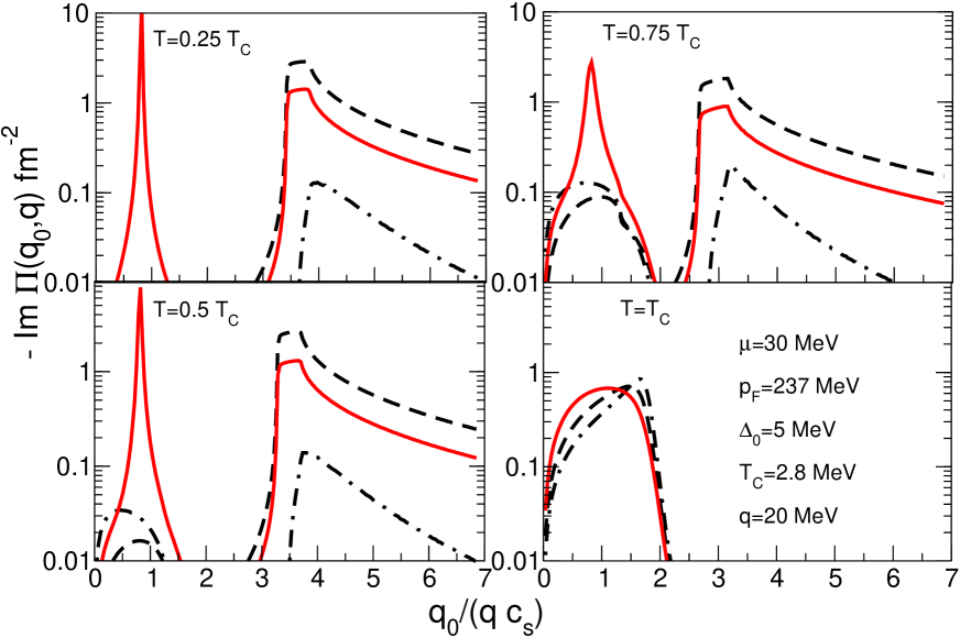
Figure 2: We plot -Im$\Pi$ as a function of the dimensionless variable $q_{0}/(qc_{s})$, where $c_{s}=p_{F}/(\sqrt{3}M)$ and with fixed momentum transfer $q=0.1p_{F}$. The dashed line is the quasi-free vector response, -Im$\Pi^{qf}_{V}$, and the solid line is the full RPA (that is, quasi-free plus collective with screening corrections) vector response, -Im$\Pi^{RPA}_{V}$. The spike at $q_{0}/(qc_{s})\simeq 1$ is the Goldstone mode response. The dot-dashed line is the RPA axial response, -Im$\Pi^{RPA}_{A}$. We use neutron chemical potential $\mu=p_{F}^{2}/(2M)=30$ MeV. The gap at zero temperature is $\Delta=5$ MeV, and the critical temperature is $T_{c}=2.8$ MeV.

The response in the axial vector channel can also be calculated using the method described above. In this case, the vertex does not exhibit any singular behavior, since there is no Goldstone mode in this channel. In a homogeneous and isotropic system, the axial polarization tensor is diagonal, with equal components, $\Pi^{A}_{11}=\Pi^{A}_{22}=\Pi^{A}_{33}=\Pi_{A}$. An explicit calculation shows that the axial polarization tensor in RPA is

$$\Pi_{A}^{RPA}(q_{0},\vec{q})=~{}\frac{1}{\chi_{0}}~{}\Pi_{A}^{qf}(q_{0},\vec{q})$$ (28)

where

$$\Pi_{A}^{qf}(q_{0},\vec{q})=~{}-\imath~{}\int~{}\frac{d^{4}p}{(2\pi)^{4}}~{}{\rm Tr\,}[S(p)~{}\hat{1}~{}S(p+q)~{}\hat{1}]\,.$$ (29)

The dot-dashed lines in Fig. 2 show the behavior of the imaginary part of the $\Pi_{A}^{RPA}(q_{0},\vec{q})$ at fixed q as a function of $q_{0}$.

Figure 3: We plot the differential cross section for neutral-current neutrino scattering in superfluid neutron matter as a function of the dimensionless variable $q_{0}/(qc_{s})$, where $c_{s}=p_{F}/(\sqrt{3}M)\simeq 0.15$. The solid curves are the RPA results which include the Goldstone contribution and the dashed lines are the mean-field results. The incoming neutrino energy and the momentum transfer $q$ were set equal to $\pi\times T$ - typical of thermal neutrinos. The spike at $q_{0}/(qc_{s})\simeq 1$ is the Goldstone mode response. We use neutron chemical potential $\mu=p_{F}^{2}/(2M)=30$ MeV. The gap at zero temperature is $\Delta=5$ MeV, and the critical temperature is $T_{c}=2.8$ MeV.

The differential cross section for neutrino scattering in the neutron matter can be written in terms of the imaginary part of the polarization tensor. The differential cross section per unit volume for a neutrino with energy $E_{\nu}$ to a state with energy $E^{\prime}_{\nu}=E_{\nu}-q_{0}$ and scattering angle $\theta$ is given by

$$\frac{d^{2}\sigma}{V~{}d\cos\theta~{}dE^{\prime}_{\nu}} = ~{}-\frac{G^{2}_{\mathrm{F}}}{4\pi^{3}}~{}{E^{\prime}_{\nu}}^{2}~{}\frac{1-n_{\nu}(E_{\nu}^{\prime})}{1-\exp(-q_{0}/T)}$$ (30)

$$\times \left[c_{V}^{2}~{}(1+\cos\theta)~{}\mathrm{Im}~{}\Pi^{RPA}_{V}(q_{0},q)+c_{A}^{2}~{}(3-\cos\theta)~{}\mathrm{Im}~{}\Pi^{RPA}_{A}(q_{0},q)\right]\,.$$

These expressions permit calculation of the neutrino opacity in superfluid neutron matter at arbitrary temperature. The results are shown in Fig. 3. The incoming neutrino energy $E_{\nu}$ and the momentum transfer $q$ were set equal to $\pi T$. This is typical for thermal neutrinos. Note that the Goldstone mode continues to play a role even when $T\simeq T_{c}/2$. Note also that with increasing temperature the gap equation yields smaller gaps - seen in the decreasing threshold for the quasi-free response. Although it is easy to deduce the relative importance of RPA corrections to the response from Fig. 3, we present a table to quantify the differences. The table below provides a comparison between the differential cross sections integrated over the energy transfer (area under the curves shown in Fig. 3).

T	$d\sigma_{qf}/Vdcos\theta~{}\times~{}10^{-5}$ m-1	$d\sigma_{RPA}/Vdcos\theta~{}\times~{}10^{-5}$ m-1
0.5 TC	0.1	0.5
0.85 TC	2.6	4.9
1.1 TC	12.8	12.9

Although scattering kinematics do not probe the response in the time-like region, neutrino pair production does arise from time-like fluctuations. As a result these same polarization functions can be used in calculations of the neutrino emissivities in superfluid matter - a process that is commonly referred to as the pair-breaking process Flowers:1976 .

At low temperature and low energy, the response is dominated by the Goldstone mode. In this regime it is appropriate to use the low energy effective theory involving only the Goldstone mode. The effective Lagrangian for the U(1) mode is given by

$${\cal L}_{GB}=\frac{f_{H}^{2}}{8}(\partial_{0}U\partial_{0}U^{\dagger}-c_{s}^{2}~{}\partial_{i}U\partial_{i}U^{\dagger})$$ (31)

where $U=exp(2\imath H/f_{H})$, $H$ is the Goldstone field, and $f_{H}^{2}=M~{}p_{F}/\pi^{2}$ is a low energy constant which is the equivalent of the pion decay constant in the chiral lagrangian. We can compute the coupling of the $H$ mode to the neutrinos by matching to the weak current in the microscopic theory. We find that the amplitude for the process $\nu\rightarrow H~{}\nu$ is given by Bedaque:2003wj

$$A_{\nu\rightarrow H\nu}=\frac{G_{F}}{\sqrt{2}}~{}c_{V}~{}f_{H}~{}\partial_{0}H~{}\bar{\nu}\gamma^{0}\nu\,.$$ (32)

Using Eq. (32), we can compute the differential cross section for neutrino scattering due to the “Cerenkov” process $\nu\rightarrow H\nu$ Reddy:2002xc . We find that

$$\frac{d^{2}\sigma}{V~{}d\cos\theta~{}dE^{\prime}_{\nu}}=~{}-\frac{G^{2}_{\mathrm{F}}}{4\pi^{2}}~{}f_{H}^{2}~{}c_{V}^{2}~{}{E^{\prime}_{\nu}}^{2}~{}\frac{1-n_{\nu}(E^{\prime}_{\nu})}{1-\exp(-q_{0}/T)}(1+\cos\theta)~{}q_{0}~{}\delta(q_{0}-c_{s}q)\,.$$ (33)

The low energy and low temperature limit of the RPA response should agree with the above result obtained using the effective theory. We show that this indeed the case. We begin by noting that the RPA vertex when $q_{0}\ll\Delta$ and $q\ll k_{F}$ can be written as Nambu:1960tm

$$\tilde{\Gamma_{0}}=\frac{2\Delta q_{0}}{q_{0}^{2}-c_{s}^{2}q^{2}}~{}i\tau_{2}\,.$$ (34)

Substituting this result in Eq. (25) we find for $q_{0}\geq 0$

$$\mathrm{Im}~{}\Pi_{V}^{RPA}(q_{0},q)=-\frac{Mp_{F}}{2\pi}q_{0}~{}\delta(q_{0}-c_{s}q)\,.$$ (35)

The quasi-free response is exponentially suppressed at low temperature, and using Eq. (35) it is easily verified that the differential cross section in RPA agrees with Eq. (33).

IV Response of a One-Component, Relativistic Superfluid

In the last section we argued that a consistent calculation of the medium polarization tensor must include not only the quasi-free response of the medium associated with the pair-breaking excitations, but also the collective response associated with the massless excitation $H$ arising from spontaneous breakdown of $U(1)_{B}$. We then calculated the medium polarization tensor for a one-component, non-relativistic superfluid – superfluid neutron matter. In this section we will calculate the medium polarization tensor for a one-component ultra-relativistic superfluid – as a warm up for the CFL case, and also for its own sake – including both the quasi-free response and the collective response associated with the Goldstone mode.

The interactions of interest are

$${\mathcal{L}}_{int}={\mathcal{L}}_{Z}+{\mathcal{L}}_{S}.$$ (36)

Here, ${\mathcal{L}}_{Z}$ represents the interactions of neutrinos with the medium and is given by Eqs. (12,13). For concreteness we use $c_{V}=-1$ and $c_{A}=-1.23$. ${\mathcal{L}}_{S}$ represents the strong interactions in the medium that give rise to the superfluid mode $H$ associated with the breaking of $U(1)_{B}$. Since we expect these interactions to have the form $H(\bar{q}i\gamma_{5}q_{C}+\bar{q_{C}}i\gamma_{5}q)$ (see Refs. Casalbuoni:2000na ; Rho:1999xf ; Rho:2000ww ), we use a four-quark interaction $(\bar{q}i\gamma_{5}q_{C}+\bar{q_{C}}i\gamma_{5}q)^{2}.$ To express this in terms of Nambu-Gor’kov spinors, we define

$$\Gamma_{H}\equiv\left(\begin{array}[]{cc}0&i\gamma_{5}\\ i\gamma_{5}&0\end{array}\right).$$ (39)

Then the relevant quark self-interactions are

$$\mathcal{L}_{S}=G\;(\bar{\Psi}\Gamma_{H}\Psi)^{2}.$$ (40)

We will calculate two contributions to the medium polarization tensor, depicted in Fig. 4 using the Nambu-Gorkov propagator given in Eq. (14). Our formalism, notation and conventions closely follow those of Ref. Rischke:2000qz .

Figure 4: The two contributions to the medium polarization tensor. The first term on the right-hand side of Fig. 4 corresponds to the quasi-free response of the medium to the neutrino probe. The second term on the right-hand side corresponds to the collective response associated with the Goldstone mode $H$.

The first term on the right-hand side corresponds to the quasi-free response of the medium. The second term captures the collective response of the system associated with the superfluid excitation $H$. The collective response can be expressed as the RPA sum depicted in Fig. 5.

Figure 5: The collective response of the medium can be evaluated in the Random Phase Approximation by summing a series of diagrams.

We will first calculate the quasi-free response, then the collective response.

The quasi-free response of the medium comes from first term on the right-hand side of Fig. 4. This diagram makes the following contribution to the polarization tensor:

$$\Pi^{\mu\nu}_{qf}(Q)=$$ (41)

$$\frac{1}{2}\int\frac{d^{3}p}{(2\pi)^{3}}\left[A(E_{\bf p},E_{\bf p+q})\left\{(c_{V}^{2}+c_{A}^{2}){\cal T}^{\mu\nu}_{+}({\bf p},{\bf p+q})-2c_{V}c_{A}{\cal W}^{\mu\nu}_{+}({\bf p},{\bf p+q})\right\}\right.$$

$$\hskip 56.9055pt+A(-E_{\bf p},-E_{\bf p+q})\left\{(c_{V}^{2}+c_{A}^{2}){\cal T}^{\mu\nu}_{-}({\bf p},{\bf p+q})+2c_{V}c_{A}{\cal W}^{\mu\nu}_{-}({\bf p},{\bf p+q})\right\}$$

$$\hskip 56.9055pt-\Delta^{2}B(E_{\bf p},E_{\bf p+q})\left\{(c_{V}^{2}+c_{A}^{2})[{\cal U}^{\mu\nu}_{+}({\bf p},{\bf p+q})+{\cal U}^{\mu\nu}_{-}({\bf p},{\bf p+q})]\right.$$

$$\hskip 142.26378pt+\left.\left.2c_{V}c_{A}[{\cal V}^{\mu\nu}_{+}({\bf p},{\bf p+q})-{\cal V}^{\mu\nu}_{-}({\bf p},{\bf p+q})]\right\}\right].$$

The Matsubara sum led to the quantities

$$A(E^{\prime},E)=$$ (42)

$$\frac{1}{(2\xi)(2\xi^{\prime})}\{[n(\xi)-n(\xi^{\prime})]\left(\frac{(\xi-E)(\xi^{\prime}-E^{\prime})}{q_{0}+\xi-\xi^{\prime}}-\frac{(\xi+E)(\xi^{\prime}+E^{\prime})}{q_{0}-\xi+\xi^{\prime}}\right)$$

$$\hskip 42.67912pt+[1-n(\xi)-n(\xi^{\prime})]\left(\frac{(\xi+E)(\xi^{\prime}-E^{\prime})}{q_{0}-\xi-\xi^{\prime}}-\frac{(\xi-E)(\xi^{\prime}+E^{\prime})}{q_{0}+\xi+\xi^{\prime}}\right)\}$$

and

$$B(E^{\prime},E)=$$ (43)

$$\frac{1}{(2\xi)(2\xi^{\prime})}\{[n(\xi)-n(\xi^{\prime})]\left(\frac{1}{q_{0}+\xi-\xi^{\prime}}-\frac{1}{q_{0}-\xi+\xi^{\prime}}\right)$$

$$\hskip 42.67912pt+[1-n(\xi)-n(\xi^{\prime})]\left(-\frac{1}{q_{0}-\xi-\xi^{\prime}}+\frac{1}{q_{0}+\xi+\xi^{\prime}}\right)\}$$

with

$$\xi^{\prime}=\sqrt{{E^{\prime}}^{2}+\Delta^{2}}\qquad\mbox{and}\qquad\xi=\sqrt{E^{2}+\Delta^{2}}.$$

The trace over Dirac indices led to the quantities

$${\cal T}^{\mu\nu}_{\pm}({\bf p_{1}},{\bf p_{2}}) = \left\{\begin{array}[]{c@{\quad\mbox{if}\quad}c}1+{\bf\widehat{p_{1}}}\cdot{\bf\widehat{p_{2}}}&\mu=0\;\;\mbox{and}\;\;\nu=0\\ \pm({\bf\widehat{p_{1}}+\widehat{p_{2}}})^{\nu}&\mu=0\;\;\mbox{and}\;\;\nu\not=0\\ \pm({\bf\widehat{p_{1}}+\widehat{p_{2}}})^{\mu}&\mu\not=0\;\;\mbox{and}\;\;\nu=0\\ \delta^{\mu\nu}(1-{\bf\widehat{p_{1}}}\cdot{\bf\widehat{p_{2}}})+({\bf\widehat{p_{1}}})^{\mu}({\bf\widehat{p_{2}}})^{\nu}+({\bf\widehat{p_{2}}})^{\mu}({\bf\widehat{p_{1}}})^{\nu}&\mu\not=0\;\;\mbox{and}\;\;\nu\not=0\end{array}\right.$$ (48)

and

$${\cal W}^{\mu\nu}_{\pm}({\bf p_{1}},{\bf p_{2}}) = \left\{\begin{array}[]{c@{\quad\mbox{if}\quad}c}i\epsilon^{\mu\nu ab}({\bf\widehat{p_{1}}})_{a}({\bf\widehat{p_{2}}})_{b}&\mu=0\;\;\mbox{or}\;\;\nu=0\\ \mp i\epsilon^{\mu\nu 0a}({\bf\widehat{p_{1}}-\widehat{p_{2}}})_{a}&\mu\not=0\;\;\mbox{and}\;\;\nu\not=0\end{array}\right.$$ (51)

and

$${\cal U}^{\mu\nu}_{\pm}({\bf p_{1}},{\bf p_{2}}) = \left\{\begin{array}[]{c@{\quad\mbox{if}\quad}c}{\cal T}^{\mu\nu}_{\pm}({\bf p_{1}},{\bf p_{2}})&\nu=0\\ -{\cal T}^{\mu\nu}_{\pm}({\bf p_{1}},{\bf p_{2}})&\nu\not=0\end{array}\right.$$ (54)

and

$${\cal V}^{\mu\nu}_{\pm}({\bf p_{1}},{\bf p_{2}}) = \left\{\begin{array}[]{c@{\quad\mbox{for}\quad}c}-{\cal W}^{\mu\nu}_{\pm}({\bf p_{1}},{\bf p_{2}})&\nu=0\\ {\cal W}^{\mu\nu}_{\pm}({\bf p_{1}},{\bf p_{2}})&\nu\not=0\end{array}\right..$$ (57)

Details of this calculation are given in Appendix A.1.

Now we want to calculate the contribution to the polarization tensor from the superfluid mode $H$. This contribution is the sum of a series of terms, expressed diagrammatically in Fig. 5. The series is a geometric series, and its sum is expressed diagrammatically in Fig. 6.

Figure 6: The diagrams of the Random Phase Approximation are a geometric series.

The contribution of this geometric series to the polarization tensor is

$$\Pi^{\mu\nu}_{H}(Q)=-\frac{G}{2}\;\frac{I^{\mu}(Q)I^{\nu}(-Q)}{g(Q)},$$ (58)

where

$$I^{\mu}(Q) = \int\frac{d^{3}p}{(2\pi)^{3}}\;i\Delta\times$$ (59)

$$c_{V}\left[C(E_{\bf p},E_{\bf p+q})\;{\cal U}^{\mu 0}_{+}({\bf p},{\bf p+q})+C(-E_{\bf p},-E_{\bf p+q})\;{\cal U}^{\mu 0}_{-}({\bf p},{\bf p+q})\right]$$

with

$$C(E^{\prime},E) = \frac{1}{(2\xi)(2\xi^{\prime})}\{[n(\xi)-n(\xi^{\prime})]\left(\frac{E-E^{\prime}-\xi+\xi^{\prime}}{q_{0}+\xi-\xi^{\prime}}-\frac{E-E^{\prime}+\xi-\xi^{\prime}}{q_{0}-\xi+\xi^{\prime}}\right)$$ (60)

$$\hskip 19.91684pt+[1-n(\xi)-n(\xi^{\prime})]\left(-\frac{E-E^{\prime}+\xi+\xi^{\prime}}{q_{0}-\xi-\xi^{\prime}}+\frac{E-E^{\prime}-\xi-\xi^{\prime}}{q_{0}+\xi+\xi^{\prime}}\right)\},$$

and

$$g(Q) = 1+2\>G\int\frac{d^{3}p}{(2\pi)^{3}}(1+{\bf\hat{p}}\cdot{\bf\widehat{p+q}})$$ (61)

$$\times\frac{1}{(2\xi_{\bf p+q})(2\xi_{\bf p})}\{\left[n(\xi_{\bf p+q})-n(\xi_{\bf p})\right]\left(\xi_{\bf p+q}\xi_{\bf p}-E_{\bf p+q}E_{\bf p}-\Delta^{2}\right)$$

$$\hskip 128.0374pt\left(\frac{1}{q_{0}+\xi_{\bf p+q}-\xi_{\bf p}}-\frac{1}{q_{0}-\xi_{\bf p+q}+\xi_{\bf p}}\right)$$

$$\hskip 65.44142pt+\left[1-n(\xi_{\bf p+q})-n(\xi_{\bf p})\right]\left(\xi_{\bf p+q}\xi_{\bf p}+E_{\bf p+q}E_{\bf p}+\Delta^{2}\right)$$

$$\hskip 128.0374pt\left(\frac{1}{q_{0}-\xi_{\bf p+q}-\xi_{\bf p}}-\frac{1}{q_{0}+\xi_{\bf p+q}+\xi_{\bf p}}\right)\}.$$

Details of the evaluation are given in Appendix A.2. We should check that $g(Q)$ vanishes for $q_{0}=0$ and ${\bf q}=0$; this will indicate the presence of a massless excitation, namely, the $H$ boson. Setting $q_{0}=q=0$, we need

$$0=1-2\>G\int\frac{d^{3}p}{(2\pi)^{3}}\left[1-2n(\xi_{\bf p})\right]\frac{1}{\xi_{\bf p}}.$$ (62)

This easily verified by noting it is the gap equation obtained by minimizing the free energy: $\partial\Omega/\partial\Delta=0$.

In Fig. 7 we plot -Im $\Pi^{00}$ for various temperatures as a function of $q_{0}/(qc_{s})$, where $c_{s}=1/\sqrt{3}$, which is the expected velocity of the Goldstone mode. The dashed line is the quasi-free response, and the solid line is the full (that is, quasi-free plus collective) response. The momentum transferred to the medium is fixed at $q=60$ MeV. We use chemical potential $\mu=400$ MeV. The gap at zero temperature is $\Delta=50$ MeV, and the critical temperature is $T_{c}=28.3$ MeV. The upper left panel illustrates $T/T_{c}=0.50$. At this temperature the gap is $\Delta=47.9$ MeV. We find a narrow peak about $q_{0}/(qc_{s})=1$, confirming our expectation about the Goldstone mode. The threshold seen at $q_{0}/(qc_{s})=2.76$ corresponds to $q_{0}=95.8~{}\mbox{MeV}=2\Delta$. The middle panel illustrates $T/T_{c}=0.85$. At this temperature the gap is $\Delta=32.2$ MeV. The peak associated with the Goldstone mode has widened, and its height has shrunk relative to the response at $q_{0}=2\Delta$. Also note the nonzero response for $q_{0}/(qc_{s})\leq 1.73$, corresponding to $q_{0}\leq q$. The rightmost panel illustrates $T/T_{c}=1.10$. At this temperature the gap is $\Delta=0$. Only the $q_{0}\leq q$ response is seen, as expected.

Figure 7: We plot -Im$\Pi^{00}$ for a one-component, relativistic superfluid at various temperatures, as a function of the dimensionless variable $q_{0}/(qc_{s})$, where $c_{s}=1/\sqrt{3}$, with fixed $q=60$ MeV. The dashed line is the quasi-free response, and the solid line is the full (that is, quasi-free plus collective) response. We use chemical potential $\mu=400$ MeV. The gap at zero temperature is $\Delta=50$ MeV, and the critical temperature is $T_{c}=28.3$ MeV.

Having studied the medium polarization tensor for a one-component, relativistic superfluid, we turn to the case of a multi-component, relativistic superfluid – color-flavor locked quark matter (CFL).

V Response of CFL

We finally study CFL. The interactions can still be written as Eq. (36), except that for three-flavor quark matter we should use

$$c_{V}=\left(\begin{array}[]{ccc}\frac{1}{2}-\frac{4}{3}\sin^{2}\theta_{W}&0&0\\ 0&-\frac{1}{2}+\frac{2}{3}\sin^{2}\theta_{W}&0\\ 0&0&-\frac{1}{2}+\frac{2}{3}\sin^{2}\theta_{W}\end{array}\right),$$ (66)

where the weak mixing angle is $\sin^{2}\theta_{W}\approx 0.231$, and

$$c_{A}=\left(\begin{array}[]{ccc}\frac{1}{2}&0&0\\ 0&-\frac{1}{2}&0\\ 0&0&-\frac{1}{2}\end{array}\right).$$ (70)

Also, the four-quark interaction that gives rise to the $H$ in CFL is

$${\mathcal{L}}_{S}=G(\bar{\Psi}\Gamma_{H}\Psi)^{2},$$ (71)

using

$$\Gamma_{H}=\left(\begin{array}[]{cc}0&i\gamma_{5}M\\ i\gamma_{5}M&0\end{array}\right)\qquad\mbox{with}\qquad(M)^{cd}_{fg}=\epsilon^{cdI}\;\epsilon^{fgI},$$ (74)

where $c,d$ are color indices, and $f,g$ are flavor indices. In CFL the nine quarks form an octet with gap $\Delta_{8}\equiv\Delta$ and a singlet with gap $\Delta_{1}\equiv 2\Delta.$ We are neglecting condensation in the color ${\bf 6}$ channel, keeping only the condensate in the ${\bf\bar{3}}$ channel. The propagator involves the energies $\xi_{m\;{\bf p}}=\sqrt{(p-\mu)^{2}+\Delta_{m}^{2}}.$ The propagator also involves the following color-flavor matrices:

$$({\bf P_{1}})^{cd}_{fg}=({\bf\tilde{P}_{1}})^{cd}_{fg}=\frac{1}{3}\delta^{c}_{f}\delta^{d}_{g},~{}~{}~{}({\bf P_{8}})^{cd}_{fg}=\delta_{fg}\delta^{cd}-\frac{1}{3}\delta^{c}_{f}\delta^{d}_{g},~{}~{}~{}\mbox{and}~{}~{}~{}({\bf\tilde{P}_{8}})^{cd}_{fg}=-\delta^{d}_{f}\delta^{c}_{g}+\frac{1}{3}\delta^{c}_{f}\delta^{d}_{g}.$$

Now we can write down the quark propagator:

$$S(P)=\left(\begin{array}[]{cc}G^{+}(P)&\Xi^{-}(P)\\ \Xi^{+}(P)&G^{-}(P)\end{array}\right),$$

where

$$G^{+}(P)=\left\{\frac{{\bf P_{1}}}{p_{0}^{2}-\xi_{1\;{\bf p}}^{2}}+\frac{{\bf P_{8}}}{p_{0}^{2}-\xi_{8\;{\bf p}}^{2}}\right\}(p_{0}+E_{\bf p})\Lambda^{+}_{\bf p}\gamma_{0},$$

$$G^{-}(P)=\left\{\frac{{\bf P_{1}}}{p_{0}^{2}-\xi_{1\;{\bf p}}^{2}}+\frac{{\bf P_{8}}}{p_{0}^{2}-\xi_{8\;{\bf p}}^{2}}\right\}(p_{0}-E_{\bf p})\Lambda^{-}_{\bf p}\gamma_{0},$$

$$\Xi^{+}(P)=-\left\{\frac{\Delta_{1}{\bf\tilde{P}_{1}}}{p_{0}^{2}-\xi^{2}_{1\;{\bf p}}}+\frac{\Delta_{8}{\bf\tilde{P}_{8}}}{p_{0}^{2}-\xi^{2}_{8\;{\bf p}}}\right\}\gamma_{5}\Lambda^{-}_{\bf p},$$

and

$$\Xi^{-}(P)=\left\{\frac{\Delta_{1}{\bf\tilde{P}_{1}}}{p_{0}^{2}-\xi^{2}_{1\;{\bf p}}}+\frac{\Delta_{8}{\bf\tilde{P}_{8}}}{p_{0}^{2}-\xi^{2}_{8\;{\bf p}}}\right\}\gamma_{5}\Lambda^{+}_{\bf p}.$$

We have neglected the contribution from antiquarks.

We now calculate the contributions to the medium polarization tensor from the quasi-free response and the collective response, the two terms depicted on the right-hand side of Fig. 4.

The quasi-free contribution to the polarization tensor comes from the first term on the right-hand side of Fig. 4, and its value is

$$\Pi^{\mu\nu}_{qf}(Q) = \frac{1}{2}\int\frac{d^{3}p}{(2\pi)^{3}}\sum_{m,n\in\{1,8\}}\left(\bar{A}(E_{\bf p},E_{\bf p+q},\Delta_{m},\Delta_{n})\left\{R^{(1)}_{mn}\;{\cal T}^{\mu\nu}_{+}({\bf p},{\bf p+q})-R^{(2)}_{mn}\;{\cal W}^{\mu\nu}_{+}({\bf p},{\bf p+q})\right\}\right.$$

$$\hskip 85.35826pt+\bar{A}(-E_{\bf p},-E_{\bf p+q},\Delta_{m},\Delta_{n})\left\{R^{(1)}_{mn}\;{\cal T}^{\mu\nu}_{-}({\bf p},{\bf p+q})+R^{(2)}_{mn}\;{\cal W}^{\mu\nu}_{-}({\bf p},{\bf p+q})\right\}$$

$$\hskip 85.35826pt-\Delta_{m}\Delta_{n}\bar{B}(E_{\bf p},E_{\bf p+q},\Delta_{m},\Delta_{n})\left\{\tilde{R}^{(1)}_{mn}\;[{\cal U}^{\mu\nu}_{+}({\bf p},{\bf p+q})+{\cal U}^{\mu\nu}_{-}({\bf p},{\bf p+q})]\right.$$

$$\hskip 213.39566pt+\left.\left.\tilde{R}^{(2)}_{mn}\;[{\cal V}^{\mu\nu}_{+}({\bf p},{\bf p+q})-{\cal V}^{\mu\nu}_{-}({\bf p},{\bf p+q})]\right\}\right).$$

The Matsubara sum led to the quantities $\bar{A}$ and $\bar{B}$, where

$$\bar{A}(E^{\prime},E,\Delta^{\prime},\Delta)=$$ (76)

$$\frac{1}{(2\xi)(2\xi^{\prime})}\{[n(\xi)-n(\xi^{\prime})]\left(\frac{(\xi-E)(\xi^{\prime}-E^{\prime})}{q_{0}+\xi-\xi^{\prime}}-\frac{(\xi+E)(\xi^{\prime}+E^{\prime})}{q_{0}-\xi+\xi^{\prime}}\right)$$

$$\hskip 42.67912pt+[1-n(\xi)-n(\xi^{\prime})]\left(\frac{(\xi+E)(\xi^{\prime}-E^{\prime})}{q_{0}-\xi-\xi^{\prime}}-\frac{(\xi-E)(\xi^{\prime}+E^{\prime})}{q_{0}+\xi+\xi^{\prime}}\right)\}$$

and

$$\bar{B}(E^{\prime},E,\Delta^{\prime},\Delta)=$$ (77)

$$\frac{1}{(2\xi)(2\xi^{\prime})}\{[n(\xi)-n(\xi^{\prime})]\left(\frac{1}{q_{0}+\xi-\xi^{\prime}}-\frac{1}{q_{0}-\xi+\xi^{\prime}}\right)$$

$$+[1-n(\xi)-n(\xi^{\prime})]\left(-\frac{1}{q_{0}-\xi-\xi^{\prime}}+\frac{1}{q_{0}+\xi+\xi^{\prime}}\right)\}$$

with

$$\xi^{\prime}=\sqrt{(E^{\prime})^{2}+(\Delta^{\prime})^{2}}\qquad\mbox{and}\qquad\xi=\sqrt{E^{2}+\Delta^{2}}.$$

The trace over color-flavor indices led to the quantities

$$R^{(1)}_{mn}=\left(\begin{array}[]{cc}0.0556&0.2865\\ 0.2865&2.4502\end{array}\right)\,,\quad R^{(2)}_{mn}=\left(\begin{array}[]{cc}0.0556&0.2391\\ 0.2391&2.1182\end{array}\right)\,,$$

$$\tilde{R}^{(1)}_{mn}=\left(\begin{array}[]{cc}0.0556&-0.2865\\ -0.2865&-0.1286\end{array}\right)\,,\;\;\mbox{and}\;\;\;\tilde{R}^{(2)}_{mn}=\left(\begin{array}[]{cc}0.0556&-0.2391\\ -0.2391&-0.0338\end{array}\right)\,.$$ (78)

Note that these matrices include off-diagonal components: the weak interactions can scatter the singlet fermionic quasi-particle into one of the octet fermionic quasi-particles, and vice-versa. We discuss the color-flavor trace further in Appendix B.1.

We now want to calculate the contribution to the quark polarization tensor from the collective response of the medium. This is depicted in Fig. 6. Its value is

$$\Pi^{\mu\nu}_{H}(Q)=-\frac{G}{2}\;\frac{\bar{I}^{\mu}(Q)\bar{I}^{\nu}(-Q)}{\bar{g}(Q)},$$ (79)

where

$$\bar{I}^{\mu}(Q) = \int\frac{d^{3}p}{(2\pi)^{3}}\sum_{m\in\{1,8\}}i\Delta_{m}\;R^{(3)}_{m}\left[\bar{C}(E_{\bf p},E_{\bf p+q},\xi_{m\;{\bf p}},\xi_{m\;{\bf p+q}})\;{\cal U}^{\mu 0}_{+}({\bf p},{\bf p+q})\right.$$ (80)

$$\hskip 120.92421pt+\left.\bar{C}(-E_{\bf p},-E_{\bf p+q},\xi_{m\;{\bf p}},\xi_{m\;{\bf p+q}})\;{\cal U}^{\mu 0}_{-}({\bf p},{\bf p+q})\right],$$

with

$$\bar{C}(E^{\prime},E,\xi^{\prime},\xi)=$$ (81)

$$\frac{1}{(2\xi)(2\xi^{\prime})}\{[n(\xi)-n(\xi^{\prime})]\left(\frac{-E+E^{\prime}+\xi-\xi^{\prime}}{q_{0}+\xi-\xi^{\prime}}-\frac{-E+E^{\prime}-\xi+\xi^{\prime}}{q_{0}-\xi+\xi^{\prime}}\right)$$

$$\hskip 42.67912pt+[1-n(\xi)-n(\xi^{\prime})]\left(-\frac{-E+E^{\prime}-\xi-\xi^{\prime}}{q_{0}-\xi-\xi^{\prime}}+\frac{-E+E^{\prime}+\xi+\xi^{\prime}}{q_{0}+\xi+\xi^{\prime}}\right)\}.$$

The quantity $R^{(3)}_{m}$ arises from the color-flavor trace. Its value is

$$R^{(3)}_{1}=-\frac{1}{3}\qquad\mbox{and}\qquad R^{(3)}_{8}=-\frac{4}{3}.$$ (82)

Also,

$$\bar{g}(Q)=1+2\;G\int\frac{d^{3}p}{(2\pi)^{3}}(1+{\bf\hat{p}}\cdot{\bf\widehat{p+q}})\sum_{m}\bar{D}(E_{\bf p},E_{\bf p+q},\Delta_{m})\;R^{(5)}_{m},$$ (83)

where

$$\bar{D}(E^{\prime},E,\Delta)=$$ (84)

$$\frac{1}{(2\xi)(2\xi^{\prime})}\left\{[n(\xi)-n(\xi^{\prime})](\xi\xi^{\prime}-EE^{\prime}-\Delta^{2})\left(\frac{1}{q_{0}+\xi-\xi^{\prime}}-\frac{1}{q_{0}-\xi+\xi^{\prime}}\right)\right.$$

$$\hskip 28.45274pt+\left.[1-n(\xi)-n(\xi^{\prime})](\xi\xi^{\prime}+EE^{\prime}+\Delta^{2})\left(\frac{1}{q_{0}-\xi-\xi^{\prime}}-\frac{1}{q_{0}+\xi+\xi^{\prime}}\right)\right\}.$$

and

$$R^{(5)}_{1}=4\qquad\mbox{and}\qquad R^{(5)}_{8}=8.$$ (85)

We discuss the color-flavor traces further in Appendix B.2.

The quantity $g(Q)$ should vanish when $q_{0}=q=0$ in order to describe a massless excitation. That is, we must have

$$0=1-2\;G\int\frac{d^{3}p}{(2\pi)^{3}}\left\{[1-2n(\xi_{1\;{\bf p}})]\frac{4}{\xi_{1\;{\bf p}}}+[1-2n(\xi_{8\;{\bf p}})]\frac{8}{\xi_{8\;{\bf p}}}\right\}.$$ (86)

This is the gap equation. It gives a critical temperature $T_{c}\approx 0.71\;\Delta(T=0)$, in agreement with Ref. Schmitt:2002sc .

Figure 8: We plot -Im$\Pi^{00}$ for CFL at various temperatures as a function of $q_{0}/(qc_{s})$, where $c_{s}=1/\sqrt{3}$, with fixed $q=60$ MeV. The dashed line is the quasi-free response, and the solid line is the full (that is, quasi-free plus collective) response. We use quark chemical potential $\mu=400$ MeV. The gap at zero temperature is $\Delta=50$ MeV, and the critical temperature is $T_{c}=35.7$ MeV.

In Fig. 8 we plot -Im $\Pi^{00}$ for various temperatures as a function of $q_{0}/(qc_{s})$, where $c_{s}=1/\sqrt{3}$, which is the expected velocity of the Goldstone mode. The dashed line is the quasi-free response, and the solid line is the full (that is, quasi-free plus collective) response. The momentum transferred to the medium is fixed at $q=60$ MeV. We use quark chemical potential $\mu=400$ MeV. The gap at zero temperature is $\Delta=50$ MeV, and the critical temperature is $T_{c}=35.7$ MeV. The leftmost panel illustrates $T/T_{c}=0.50$. At this temperature the gap is $\Delta=46.7$ MeV. As in the one-component case, we find a narrow peak about $q_{0}/(qc_{s})=1$, confirming our expectation about the Goldstone mode. There is a threshold at $q_{0}/(qc_{s})=2.69$, corresponding to $q_{0}=2\Delta$, and there is an additional small response for $q_{0}/(qc_{s})\leq 1.73$, that is, $q_{0}\leq q$. The CFL response function is much more busy than in the one-component case (see Fig. 7) because of additional effects at $q_{0}=\Delta,3\Delta,4\Delta$, arising from the fact that some fermionic quasi-particles in CFL matter have a gap $\Delta$ and some have a gap $2\Delta$. The upper right panel illustrates $T/T_{c}=0.85$. At this temperature the gap is $\Delta=30.0$ MeV. The peak associated with the Goldstone mode has widened, and its height has shrunk relative to the response at $q_{0}=2\Delta$, but it overlaps with the $q_{0}\leq q$ response, which has grown. The lower panel illustrates $T/T_{c}=1.10$. At this temperature the gap is $\Delta=0$. Only the $q_{0}\leq q$ response is seen, as expected.

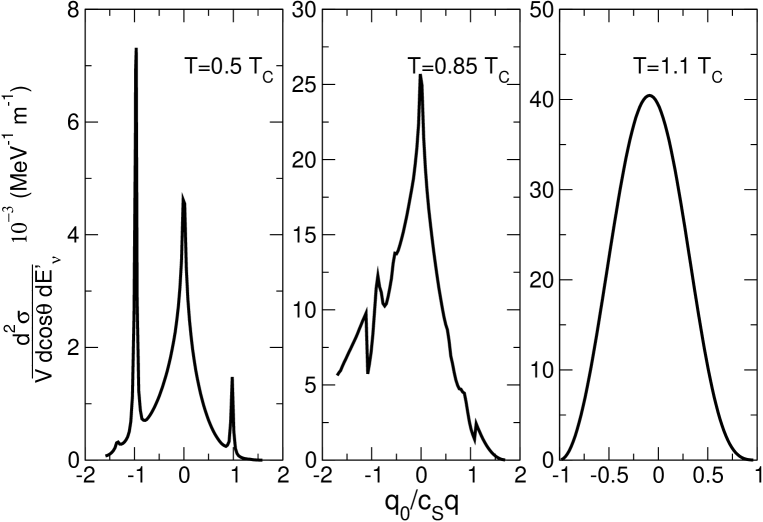
Figure 9: We plot the differential cross section for neutral-current neutrino scattering in CFL as a function of the dimensionless variable $q_{0}/(qc_{s})$, with $c_{s}=1/\sqrt{3}$ and with momentum transfer set to the typical incoming neutrino energy $q=E_{\nu}=\pi T$. The spike at $q_{0}/(qc_{s})\simeq 1$ is the Goldstone mode response. We use quark chemical potential $\mu=400$ MeV. The gap at zero temperature is $\Delta=50$ MeV, and the critical temperature is $T_{c}=35.7$ MeV.

In Fig. 9 we plot the differential cross section for neutral-current neutrino scattering in CFL. The energy of the incoming neutrino is $E_{\nu}=\pi T$, the typical energy of a thermal neutrino. The momentum transferred to the medium is set to $q=E_{\nu}$. Kinematics demand $-1.73\leq q_{0}/(qc_{s})\leq 1.73$. The parameters are otherwise as in Fig. 8. The leftmost panel is again $T/T_{c}=0.50$. There are prominent peaks near $q_{0}/(qc_{s})=\pm 1$ corresponding to the Goldstone mode. The expected feature at $q_{0}\geq 2\Delta$, corresponding to excitation of a particle-hole pair, does not lie in the kinematically allowed region of $q_{0}$. There is a small peak, however, at $q_{0}/(qc_{s})=-1.44$, or $-q_{0}=\Delta$, corresponding to scattering of a singlet quark, whose gap is $2\Delta$, into an octet quark, whose gap is $\Delta$. The middle panel illustrates $T/T_{c}=0.85$. The Goldstone peak has widened, and the threshold at $q_{0}\geq 2\Delta$ – corresponding to $q_{0}/(qc_{s})\geq 1.09$ – now falls in the kinematically allowed region. The rightmost panel illustrates $T/T_{c}=1.10$. This is the result for free quarks.

VI Conclusion

We have calculated the differential cross section for neutral-current neutrino scattering in superfluid neutron matter, plotted in Fig. 3 and in color-flavor locked quark matter, plotted in Fig. 9, under conditions relevant to proto-neutron stars. Our results apply above and below the critical temperature. In both of these regimes our model for the interaction in the medium includes the dominant contribution to the cross section. Above the critical temperature, this comes from the fermionic excitations, which become the pair-breaking excitations below the critical temperature. Well below the critical temperature the dominant contribution comes from the massless bosonic mode associated with the breaking of $U(1)$. Although we presented results results for scattering cross sections with space-like kinematics, our polarization functions extend into the time-like region where pair-breaking (and recombination) is the dominant source of the response. These could be employed in calculations of the neutrino emissivity. In particular, we have demonstrated the importance of vertex corrections in these region. Our results suggest that earlier calculations of the neutrino emissivity from the pair recominbation process in superfluid neutron matter Flowers:1976 and quark matter Jaikumar:2001hq , which ignore these vertex (RPA) corrections, need to be revised.

The analysis presented here is based on mean-field and the random phase approximation (RPA). Its validity is restricted to weak coupling, $\Delta\ll\mu$. For strong coupling we can expect the response to differ quantitatively. In particular, screening corrections which were discussed earlier could be significant. Another drawback is our use of simplified interactions to describe superfluid neutron and quark matter. Our focus was to explore the role of superfluidity and this motivated our choice of a simple zero-range s-wave interaction. In reality, the nucleon-nucleon and quark-quark interactions are more complex. These will induce additional correlations which will affect both the gap equation and the response. (For a recent review on the role of strong interaction correlations on neutrino opacities see Ref. Burrows:2004vq .) Given the non-perturbative nature of these corrections it is difficult to foresee how large they may be.

Although our results are valid both above and below the critical temperature, we have implicitly assumed that the transition is a BCS-like second order transition. Several caveats must be borne in mind when using our results near $T_{c}$. In the real system this transition may be first order either due to gauge field fluctuations Giannakis:2001wz or stresses such as the strange quark mass and electric charge neutrality Steiner:2002gx . Also, fluctuations of the magnitude of the order parameter dominate in a region called the Ginsburg region around $T_{c}$. In strong coupling, the size of this region could be significant fraction of $T_{c}$ Voskresensky:2003wd . Our approach captures some of these fluctuations through RPA. Nonetheless, a Landau-Ginsburg approach - an effective theory for $|\Delta|$, is more appropriate in this regime Iida:2000ha . In particular, there are precursor fluctuations just above $T_{c}$, which are not included in our response, that may be relevant Kitazawa:2001ft . These effects are currently under investigation and will be reported elsewhere.

Our primary goal was to provide expressions for the differential cross sections that could be used in simulations of the early thermal evolution of neutron stars born in the aftermath of a supernova explosion. The microphysics of neutrino scattering affects the rate of diffusion, which in turn affects macroscopic observables such as the cooling rate and the neutrino emission from core-collapse supernovae. Our results, which extends both to the low and high temperature regions, are well suited for use in simulations of core-collapse supernovae and early thermal evolution of neutron stars.

Acknowledgments

We would like to thank B. Fore, M. Forbes, K. Fukushima, C. Kouvaris, K. Rajagopal and G. Rupak for helpful discussions. J.K. would also like to thank the Institute for Fundamental Theory at the University of Florida for its hospitality. The research of J.K. is supported by the Department of Energy under cooperative research agreement DE-FC02-94ER40818. The research of S. R is supported by the Department of Energy under contract W-7405-ENG-36.

Appendix A Calculation of the polarization tensor for the relativistic superfluid

In this appendix we detail the calculation of the medium polarization tensor for the one-component, relativistic superfluid. In Section A.1 we evaluate the contribution from the quasi-free response function. In Section A.2 we include the contribution from the collective response.

A.1 Quasi-free response

The contribution to the medium polarization tensor can be associated with the first diagram on the right-hand side of Fig. 4. That diagram has the value

$$\Pi^{\mu\nu}_{qf}(Q)=-i\frac{1}{2}\int\frac{d^{4}P}{(2\pi)^{4}}\mbox{Tr}[\Gamma^{\mu}_{Z}S(P)\Gamma^{\nu}_{Z}S(P+Q)].$$ (87)

The factor of $\frac{1}{2}$ is due to the doubling of fermion degrees of freedom in the Nambu-Gor’kov formalism. Evaluating the trace over Nambu-Gor’kov indices gives

$$\Pi^{\mu\nu}_{qf}(Q) = -i\frac{1}{2}\int\frac{d^{4}P}{(2\pi)^{4}}\mbox{Tr}[\gamma^{\mu}(c_{V}-c_{A}\gamma_{5})G^{+}(P)\gamma^{\nu}(c_{V}-c_{A}\gamma_{5})G^{+}(P+Q)$$ (88)

$$\hskip 62.59596pt-\gamma^{\mu}(c_{V}-c_{A}\gamma_{5})\Xi^{-}(P)\gamma^{\nu}(c_{V}+c_{A}\gamma_{5})\Xi^{+}(P+Q)$$

$$\hskip 62.59596pt-\gamma^{\mu}(c_{V}+c_{A}\gamma_{5})\Xi^{+}(P)\gamma^{\nu}(c_{V}-c_{A}\gamma_{5})\Xi^{-}(P+Q)$$

$$\hskip 62.59596pt+\gamma^{\mu}(c_{V}+c_{A}\gamma_{5})G^{-}(P)\gamma^{\nu}(c_{V}+c_{A}\gamma_{5})G^{-}(P+Q)],$$

where the remaining trace is over Dirac indices. We will write down the value of each of the four traces above. First,

$$\mbox{Tr}[\gamma^{\mu}(c_{V}-c_{A}\gamma_{5})G^{+}(P)\gamma^{\nu}(c_{V}-c_{A}\gamma_{5})G^{+}(P+Q)]$$

$$= \frac{(p_{0}+E_{\bf p})(p_{0}+q_{0}+E_{\bf p+q})}{[p_{0}^{2}-\xi_{\bf p}^{2}][(p+q)_{0}^{2}-\xi_{\bf p+q}^{2}]}\left\{(c_{V}^{2}+c_{A}^{2}){\cal T}^{\mu\nu}_{+}({\bf p},{\bf p+q})-2c_{V}c_{A}{\cal W}^{\mu\nu}_{+}({\bf p},{\bf p+q})\right\},$$

where ${\cal T}^{\mu\nu}_{\pm}$ is defined by

$${\cal T}^{\mu\nu}_{\pm}({\bf p_{1}},{\bf p_{2}})=\mbox{Tr}[\gamma_{0}\gamma^{\mu}\Lambda^{\pm}_{\bf p_{1}}\gamma_{0}\gamma^{\nu}\Lambda^{\pm}_{\bf p_{2}}],$$ (89)

and ${\cal W}^{\mu\nu}_{\pm}$ is defined by

$${\cal W}^{\mu\nu}_{\pm}({\bf p_{1}},{\bf p_{2}})=\mbox{Tr}[\gamma_{0}\gamma^{\mu}\Lambda^{\pm}_{\bf p_{1}}\gamma_{0}\gamma^{\nu}\Lambda^{\pm}_{\bf p_{2}}\gamma_{5}].$$ (90)

Explicit evaluation of ${\cal T}^{\mu\nu}_{\pm}$ and ${\cal W}^{\mu\nu}_{\pm}$ gives Eqs. (48, 51), respectively. The second term in (88) is

$$\mbox{Tr}[-\gamma^{\mu}(c_{V}-c_{A}\gamma_{5})\Xi^{-}(P)\gamma^{\nu}(c_{V}+c_{A}\gamma_{5})\Xi^{+}(P+Q)]$$

$$= \frac{-\Delta^{2}}{[p_{0}^{2}-\xi_{\bf p}^{2}][(p+q)_{0}^{2}-\xi_{\bf p+q}^{2}]}\left\{(c_{V}^{2}+c_{A}^{2}){\cal U}^{\mu\nu}_{+}({\bf p},{\bf p+q})+2c_{V}c_{A}{\cal V}^{\mu\nu}_{+}({\bf p},{\bf p+q})\right\},$$

where ${\cal U}^{\mu\nu}_{\pm}$ is defined by

$${\cal U}^{\mu\nu}_{\pm}({\bf p_{1}},{\bf p_{2}})=\mbox{Tr}[\gamma^{\mu}\Lambda^{\pm}_{\bf p_{1}}\gamma^{\nu}\Lambda^{\mp}_{\bf p_{2}}],$$ (91)

and ${\cal V}^{\mu\nu}_{\pm}$ is defined by

$${\cal V}^{\mu\nu}_{\pm}({\bf p_{1}},{\bf p_{2}})=\mbox{Tr}[\gamma_{0}\gamma^{\mu}\Lambda^{\pm}_{\bf p_{1}}\gamma_{0}\gamma^{\nu}\Lambda^{\pm}_{\bf p_{2}}\gamma_{5}].$$ (92)

Explicit evaulation of ${\cal U}^{\mu\nu}_{\pm}$ and ${\cal V}^{\mu\nu}_{\pm}$ gives Eqs. (54, 57), respectively. The third term in (88) is

$$\mbox{Tr}[-\gamma^{\mu}(c_{V}+c_{A}\gamma_{5})\Xi^{+}(P)\gamma^{\nu}(c_{V}-c_{A}\gamma_{5})\Xi^{-}(P+Q)]$$

$$= \frac{-\Delta^{2}}{[p_{0}^{2}-\xi_{\bf p}^{2}][(p+q)_{0}^{2}-\xi_{\bf p+q}^{2}]}\left\{(c_{V}^{2}+c_{A}^{2}){\cal U}^{\mu\nu}_{-}({\bf p},{\bf p+q})-2c_{V}c_{A}{\cal V}^{\mu\nu}_{-}({\bf p},{\bf p+q})\right\}.$$

And the final term in (88) is

$$\mbox{Tr}[\gamma^{\mu}(c_{V}+c_{A}\gamma_{5})G^{-}(P)\gamma^{\nu}(c_{V}+c_{A}\gamma_{5})G^{-}(P+Q)]$$

$$= \frac{(p_{0}-E_{\bf p})(p_{0}+q_{0}-E_{\bf p+q})}{[p_{0}^{2}-\xi_{\bf p}^{2}][(p+q)_{0}^{2}-\xi_{\bf p+q}^{2}]}\left\{(c_{V}^{2}+c_{A}^{2}){\cal T}^{\mu\nu}_{-}({\bf p},{\bf p+q})+2c_{V}c_{A}{\cal W}^{\mu\nu}_{-}({\bf p},{\bf p+q})\right\}.$$

Next, we consider the Matsubara sums:

$$A(E^{\prime},E)=\frac{1}{\beta}\sum_{n}\frac{(p_{0}+q_{0}+E)(p_{0}+E^{\prime})}{[(p_{0}+q_{0})^{2}-\xi^{2}][p_{0}^{2}-\xi^{\prime 2}]}$$ (93)

and

$$B(E^{\prime},E)=\frac{1}{\beta}\sum_{n}\frac{1}{[(p_{0}+q_{0})^{2}-\xi^{2}][p_{0}^{2}-\xi^{\prime 2}]},$$ (94)

where $p_{0}=-i(2n+1)\pi/\beta$ is a fermionic Matsubara frequency; $q_{0}=-i2m\pi/\beta$ is a bosonic Matsubara frequency; and

$$\xi^{\prime}=\sqrt{{E^{\prime}}^{2}+\Delta^{2}}\qquad\mbox{and}\qquad\xi=\sqrt{E^{2}+\Delta^{2}}.$$

Explicit expressions for $A$ and $B$ are given in Eqs. (42, 43), respectively. Adding all the terms yields Eq. (41).

A.2 Collective response

In this section we detail the evaluation of the quantity depicted on the right-hand side of Fig. 6, corresponding to the collective response of the medium. First we evaluate the numerator of that quantity, then the denominator.

A.2.1 The numerator

The numerator of the right-hand side of Fig. 6 contributes

$$-G\>2\>{1\over 2}\>{1\over 2}\int\frac{d^{4}P}{(2\pi)^{4}}\frac{d^{4}K}{(2\pi)^{4}}\mbox{Tr}[\Gamma^{\mu}_{Z}S(P)\Gamma_{H}S(P+Q)]\;\mbox{Tr}[\Gamma_{H}S(K)\Gamma^{\nu}_{Z}S(K+Q)]=$$

$$-\frac{G}{2}I^{\mu}(Q)I^{\nu}(-Q),$$

where

$$I^{\mu}(Q) \equiv \int\frac{d^{4}P}{(2\pi)^{4}}\mbox{Tr}[\Gamma^{\mu}_{Z}S(P)\Gamma_{H}S(P+Q)].$$ (95)

To evaluate $I^{\mu}(Q)$ we first compute

$$\mbox{Tr}[\Gamma^{\mu}_{Z}S(P)\Gamma_{H}S(P+Q)]$$

$$= \mbox{Tr}[\left(\begin{array}[]{cc}\gamma^{\mu}(c_{V}-c_{A}\gamma_{5})&0\\ 0&-\gamma^{\mu}(c_{V}+c_{A}\gamma_{5})\end{array}\right)\left(\begin{array}[]{cc}G^{+}(P)&\Xi^{-}(P)\\ \Xi^{+}(P)&G^{-}(P)\end{array}\right)$$

$$\hskip 14.22636pt\left(\begin{array}[]{cc}0&i\gamma_{5}\\ i\gamma_{5}&0\end{array}\right)\left(\begin{array}[]{cc}G^{+}(P+Q)&\Xi^{-}(P+Q)\\ \Xi^{+}(P+Q)&G^{-}(P+Q)\end{array}\right)]$$

$$= \mbox{Tr}[i\gamma^{\mu}(c_{V}-c_{A}\gamma_{5})G^{+}(P)\gamma_{5}\Xi^{+}(P+Q)$$

$$\hskip 14.22636pt+i\gamma^{\mu}(c_{V}-c_{A}\gamma_{5})\Xi^{-}(P)\gamma_{5}G^{+}(P+Q)$$

$$\hskip 14.22636pt-i\gamma^{\mu}(c_{V}+c_{A}\gamma_{5})\Xi^{+}(P)\gamma_{5}G^{-}(P+Q)$$

$$\hskip 14.22636pt-i\gamma^{\mu}(c_{V}+c_{A}\gamma_{5})G^{-}(P)\gamma_{5}\Xi^{-}(P+Q)].$$

Now,

$$\mbox{Tr}[i\gamma^{\mu}(c_{V}-c_{A}\gamma_{5})G^{+}(P)\gamma_{5}\Xi^{+}(P+Q)]$$

$$= \frac{(p_{0}+E_{\bf p})(-i\Delta)}{[p_{0}^{2}-\xi_{\bf p}^{2}][(p+q)_{0}^{2}-\xi_{\bf p+q}^{2}]}\left[c_{V}{\cal U}^{\mu 0}_{+}({\bf p},{\bf p+q})+c_{A}{\cal V}^{\mu 0}_{+}({\bf p},{\bf p+q})\right].$$

Next,

$$\mbox{Tr}[i\gamma^{\mu}(c_{V}-c_{A}\gamma_{5})\Xi^{-}(P)\gamma_{5}G^{+}(P+Q)]$$

$$= \frac{(i\Delta)((p+q)_{0}+E_{\bf p+q})}{[p_{0}^{2}-\xi_{\bf p}^{2}][(p+q)_{0}^{2}-\xi_{\bf p+q}^{2}]}\left[c_{V}{\cal U}^{\mu 0}_{+}({\bf p},{\bf p+q})+c_{A}{\cal V}^{\mu 0}_{+}({\bf p},{\bf p+q})\right].$$

And

$$\mbox{Tr}[-i\gamma^{\mu}(c_{V}+c_{A}\gamma_{5})\Xi^{+}(P)\gamma_{5}G^{-}(P+Q)]$$

$$= \frac{(i\Delta)((p+q)_{0}-E_{\bf p+q})}{[p_{0}^{2}-\xi_{\bf p}^{2}][(p+q)_{0}^{2}-\xi_{\bf p+q}^{2}]}\left[c_{V}{\cal U}^{\mu 0}_{-}({\bf p},{\bf p+q})-c_{A}{\cal V}^{\mu 0}_{-}({\bf p},{\bf p+q})\right].$$

Finally,

$$\mbox{Tr}[-i\gamma^{\mu}(c_{V}+c_{A}\gamma_{5})G^{-}(P)\gamma_{5}\Xi^{-}(P+Q)]$$

$$= \frac{(p_{0}-E_{\bf p})(-i\Delta)}{[p_{0}^{2}-\xi_{\bf p}^{2}][(p+q)_{0}^{2}-\xi_{\bf p+q}^{2}]}\left[c_{V}{\cal U}^{\mu 0}_{-}({\bf p},{\bf p+q})-c_{A}{\cal V}^{\mu 0}_{-}({\bf p},{\bf p+q})\right].$$

To proceed we evaluate the Matsubara sums

$$C_{1}(E^{\prime},E) \equiv \frac{1}{\beta}\sum_{n}\frac{p_{0}+E^{\prime}}{[(p_{0}+q_{0})^{2}-\xi^{2}][p_{0}^{2}-\xi^{\prime 2}]}$$

$$= \frac{1}{(2\xi)(2\xi^{\prime})}\{[n(\xi)-n(\xi^{\prime})]\left(-\frac{\xi^{\prime}-E^{\prime}}{q_{0}+\xi-\xi^{\prime}}-\frac{\xi^{\prime}+E^{\prime}}{q_{0}-\xi+\xi^{\prime}}\right)$$

$$\hskip 42.67912pt+[1-n(\xi)-n(\xi^{\prime})]\left(\frac{\xi^{\prime}-E^{\prime}}{q_{0}-\xi-\xi^{\prime}}+\frac{\xi^{\prime}+E^{\prime}}{q_{0}+\xi+\xi^{\prime}}\right)\}$$

and

$$C_{2}(E^{\prime},E) \equiv \frac{1}{\beta}\sum_{n}\frac{p_{0}+q_{0}+E}{[(p_{0}+q_{0})^{2}-\xi^{2}][p_{0}^{2}-\xi^{\prime 2}]}$$

$$= \frac{1}{(2\xi)(2\xi^{\prime})}\{[n(\xi)-n(\xi^{\prime})]\left(-\frac{\xi-E}{q_{0}+\xi-\xi^{\prime}}-\frac{\xi+E}{q_{0}-\xi+\xi^{\prime}}\right)$$

$$\hskip 42.67912pt+[1-n(\xi)-n(\xi^{\prime})]\left(-\frac{\xi+E}{q_{0}-\xi-\xi^{\prime}}-\frac{\xi-E}{q_{0}+\xi+\xi^{\prime}}\right)\}$$

If we define

$$C(E^{\prime},E) \equiv -C_{1}(E^{\prime},E)+C_{2}(E^{\prime},E)$$

$$= \frac{1}{(2\xi)(2\xi^{\prime})}\{[n(\xi)-n(\xi^{\prime})]\left(\frac{E-E^{\prime}-\xi+\xi^{\prime}}{q_{0}+\xi-\xi^{\prime}}-\frac{E-E^{\prime}+\xi-\xi^{\prime}}{q_{0}-\xi+\xi^{\prime}}\right)$$

$$\hskip 19.91684pt+[1-n(\xi)-n(\xi^{\prime})]\left(-\frac{E-E^{\prime}+\xi+\xi^{\prime}}{q_{0}-\xi-\xi^{\prime}}+\frac{E-E^{\prime}-\xi-\xi^{\prime}}{q_{0}+\xi+\xi^{\prime}}\right)\},$$

then an expression for $I^{\mu}$ is

$$I^{\mu}(Q) = \int\frac{d^{3}p}{(2\pi)^{3}}\;i\Delta\times$$

$$\left\{C(E_{\bf p},E_{\bf p+q})[c_{V}{\cal U}^{\mu 0}_{+}({\bf p},{\bf p+q})+c_{A}{\cal V}^{\mu 0}_{+}({\bf p},{\bf p+q})]\right.$$

$$+\left.C(-E_{\bf p},-E_{\bf p+q})[c_{V}{\cal U}^{\mu 0}_{-}({\bf p},{\bf p+q})-c_{A}{\cal V}^{\mu 0}_{-}({\bf p},{\bf p+q})]\right\}.$$

After performing the $\int d^{3}p$ integral, the terms proportional to $c_{A}$ vanish, leaving

$$I^{\mu}(Q) = \int\frac{d^{3}p}{(2\pi)^{3}}\;i\Delta\;c_{V}\left[C(E_{\bf p},E_{\bf p+q})\;{\cal U}^{\mu 0}_{+}({\bf p},{\bf p+q})+C(-E_{\bf p},-E_{\bf p+q})\;{\cal U}^{\mu 0}_{-}({\bf p},{\bf p+q})\right].$$

This is Eq. (59).

A.2.2 The denominator

In this section we evaluate the denominator of the right-hand side of Fig. 6. It has the value

$$g(Q) \equiv 1+G\>2\>\frac{1}{2}\int\frac{d^{4}P}{(2\pi)^{4}}\mbox{Tr}[S(P+Q)\Gamma_{H}S(P)\Gamma_{H}]$$

$$= 1+G\>2\>\frac{1}{2}\int\frac{d^{4}P}{(2\pi)^{4}}\mbox{Tr}[S(P+Q)\Gamma_{H}S(P)\Gamma_{H}]$$

$$= 1+G\int\frac{d^{4}P}{(2\pi)^{4}}\mbox{Tr}[\left(\begin{array}[]{cc}G^{+}(P+Q)&\Xi^{-}(P+Q)\\ \Xi^{+}(P+Q)&G^{-}(P+Q)\end{array}\right)\left(\begin{array}[]{cc}0&i\gamma_{5}\\ i\gamma_{5}&0\end{array}\right)$$

$$\hskip 85.35826pt\left(\begin{array}[]{cc}G^{+}(P)&\Xi^{-}(P)\\ \Xi^{+}(P)&G^{-}(P)\end{array}\right)\left(\begin{array}[]{cc}0&i\gamma_{5}\\ i\gamma_{5}&0\end{array}\right)]$$

$$= 1-G\int\frac{d^{4}P}{(2\pi)^{4}}\mbox{Tr}[\Xi^{-}(P+Q)\gamma_{5}\Xi^{-}(P)\gamma_{5}+G^{+}(P+Q)\gamma_{5}G^{-}(P)\gamma_{5}$$

$$\hskip 76.82234pt+G^{-}(P+Q)\gamma_{5}G^{+}(P)\gamma_{5}+\Xi^{+}(P+Q)\gamma_{5}\Xi^{+}(P)\gamma_{5}]$$

$$= 1+G\int\frac{d^{4}P}{(2\pi)^{4}}(1+{\bf\hat{p}}\cdot{\bf\widehat{p+q}})$$

$$\times\frac{((p+q)_{0}+E_{\bf p+q})(p_{0}-E_{\bf p})-\Delta^{2}+((p+q)_{0}-E_{\bf p+q})(p_{0}+E_{\bf p})-\Delta^{2}}{[(p+q)_{0}^{2}-\xi_{\bf p+q}^{2}][p_{0}^{2}-\xi_{\bf p}^{2}]}$$

$$= 1+2\>G\int\frac{d^{3}p}{(2\pi)^{3}}(1+{\bf\hat{p}}\cdot{\bf\widehat{p+q}})$$

$$\times\frac{1}{(2\xi_{\bf p})(2\xi_{\bf p+q})}\{\left[n(\xi_{\bf p})-n(\xi_{\bf p+q})\right]\left(\xi_{\bf p+q}\xi_{\bf p}-E_{\bf p+q}E_{\bf p}-\Delta^{2}\right)$$

$$\hskip 128.0374pt\left(\frac{1}{q_{0}+\xi_{\bf p}-\xi_{\bf p+q}}-\frac{1}{q_{0}-\xi_{\bf p}+\xi_{\bf p+q}}\right)$$

$$\hskip 65.44142pt+\left[1-n(\xi_{\bf p})-n(\xi_{\bf p+q})\right]\left(\xi_{\bf p+q}\xi_{\bf p}+E_{\bf p+q}E_{\bf p}+\Delta^{2}\right)$$

$$\hskip 128.0374pt\left(\frac{1}{q_{0}-\xi_{\bf p}-\xi_{\bf p+q}}-\frac{1}{q_{0}+\xi_{\bf p}+\xi_{\bf p+q}}\right)\}.$$

This is Eq. (61).

Appendix B Color-flavor traces in the polarization tensor for CFL

In Appendix A we evaluated the polarization tensor for the one-component, relativistic superfluid. This involved traces over Nambu-Gor’kov and Dirac indices, as well as a sum over Matsubara frequencies. Similar calculations are required to evaluate the polarization tensor for CFL. The two gap color-flavor structure of the quark propagator complicates things. We discuss in this appendix the color-flavor traces that must be computed to evaluate the CFL polarization tensor. First we discuss the color-flavor traces involved in the evaluation of the quasi-free response, and then we discuss the color-flavor traces involved in the evaluation of the collective response.

B.1 Quasi-free response

The contribution to the polarization tensor from the quasi-free response of the medium comes from the first term on the right-hand side of Fig. 6. Evaluating this diagram involves a trace over Nambu-Gor’kov and Dirac indices, as well as a Matsubara sum – these calculations are similar to those in the relativistic case. The complication in the present case comes from the trace over color-flavor indices, due to the two gap structure of CFL. The color-flavor trace involves the quantities

$$R^{(1)}_{mn}=\mbox{Tr}[c_{V}{\bf P_{m}}c_{V}{\bf P_{n}}]+\mbox{Tr}[c_{A}{\bf P_{m}}c_{A}{\bf P_{n}}],$$

$$R^{(2)}_{mn}=\mbox{Tr}[c_{V}{\bf P_{m}}c_{A}{\bf P_{n}}]+\mbox{Tr}[c_{A}{\bf P_{m}}c_{V}{\bf P_{n}}],$$

$$\tilde{R}^{(1)}_{mn}=\mbox{Tr}[c_{V}{\bf\tilde{P}_{m}}c_{V}{\bf\tilde{P}_{n}}]+\mbox{Tr}[c_{A}{\bf\tilde{P}_{m}}c_{A}{\bf\tilde{P}_{n}}],$$

and

$$\tilde{R}^{(2)}_{mn}=\mbox{Tr}[c_{V}{\bf\tilde{P}_{m}}c_{A}{\bf\tilde{P}_{n}}]+\mbox{Tr}[c_{A}{\bf\tilde{P}_{m}}c_{V}{\bf\tilde{P}_{n}}].$$

Explicit values for these quantities are given in Eq. (78).

B.2 Collective response

We now want to calculate the contribution to the quark polarization tensor from the collective response associated with the $H$ boson, depicted in Fig. 6. The color-flavor traces involved in calculating this contribution are much simpler than those involved in calculating the quasi-free response, since the $H$-quark coupling does not mix the singlet and octet quasi-quarks. To evaluate the numerator of Fig. 6, we only need the coefficients

$$R^{(3)}_{m}=\mbox{Tr}[c_{V}{\bf P_{m}}M{\bf\tilde{P}_{m}}]=\mbox{Tr}[c_{V}{\bf\tilde{P}_{m}}M{\bf P_{m}}]=\mbox{Tr}[c_{A}{\bf P_{m}}M{\bf\tilde{P}_{m}}]=\mbox{Tr}[c_{A}{\bf\tilde{P}_{m}}M{\bf P_{m}}].$$

This is explicitly evaluated in Eq. (82). To evaluate the denominator, we only need the coefficients

$$R^{(5)}_{m}=\mbox{Tr}[M{\bf P_{m}}M{\bf P_{m}}]=\mbox{Tr}[M{\bf\tilde{P}_{m}}M{\bf\tilde{P}_{m}}].$$

This is explicitly evaluated in Eq. (85).

References

• (1) B. C. Barrois, Nucl. Phys. B129, 390 (1977).
• (2) D. Bailin and A. Love, Phys. Rept. 107, 325 (1984).
• (3) M. G. Alford, K. Rajagopal, and F. Wilczek, Phys. Lett. B422, 247 (1998), hep-ph/9711395.
• (4) R. Rapp, T. Schafer, E. V. Shuryak, and M. Velkovsky, Phys. Rev. Lett. 81, 53 (1998), hep-ph/9711396.
• (5) M. G. Alford, K. Rajagopal, and F. Wilczek, Nucl. Phys. B537, 443 (1999), hep-ph/9804403.
• (6) P. F. Bedaque and T. Schafer, Nucl. Phys. A697, 802 (2002), hep-ph/0105150.
• (7) D. B. Kaplan and S. Reddy, Phys. Rev. D65, 054042 (2002), hep-ph/0107265.
• (8) M. G. Alford, J. A. Bowers, and K. Rajagopal, Phys. Rev. D63, 074016 (2001), hep-ph/0008208.
• (9) J. A. Bowers, J. Kundu, K. Rajagopal, and E. Shuster, Phys. Rev. D64, 014024 (2001), hep-ph/0101067.
• (10) A. K. Leibovich, K. Rajagopal, and E. Shuster, Phys. Rev. D64, 094005 (2001), hep-ph/0104073.
• (11) J. Kundu and K. Rajagopal, Phys. Rev. D65, 094022 (2002), hep-ph/0112206.
• (12) R. Casalbuoni, R. Gatto, M. Mannarelli, and G. Nardulli, Phys. Lett. B524, 144 (2002), hep-ph/0107024.
• (13) R. Casalbuoni, R. Gatto, and G. Nardulli, Phys. Lett. B543, 139 (2002), hep-ph/0205219.
• (14) R. Casalbuoni, E. Fabiano, R. Gatto, M. Mannarelli, and G. Nardulli, Phys. Rev. D66, 094006 (2002), hep-ph/0208121.
• (15) R. Casalbuoni, R. Gatto, M. Mannarelli, and G. Nardulli, Phys. Rev. D66, 014006 (2002), hep-ph/0201059.
• (16) M. Alford, C. Kouvaris, and K. Rajagopal, (2003), hep-ph/0311286.
• (17) M. G. Alford, J. Berges, and K. Rajagopal, Nucl. Phys. B571, 269 (2000), hep-ph/9910254.
• (18) M. Alford and S. Reddy, Phys. Rev. D67, 074024 (2003), nucl-th/0211046.
• (19) M. Baldo et al., Phys. Lett. B562, 153 (2003), nucl-th/0212096.
• (20) S. Banik and D. Bandyopadhyay, Phys. Rev. D67, 123003 (2003), astro-ph/0212340.
• (21) I. Shovkovy, M. Hanauske, and M. Huang, Phys. Rev. D67, 103004 (2003), hep-ph/0303027.
• (22) M. Buballa, F. Neumann, M. Oertel, and I. Shovkovy, (2003), nucl-th/0312078.
• (23) S. B. Ruster and D. H. Rischke, Phys. Rev. D69, 045011 (2004), nucl-th/0309022.
• (24) G. W. Carter and S. Reddy, Phys. Rev. D62, 103002 (2000), hep-ph/0005228.
• (25) P. Jaikumar and M. Prakash, Phys. Lett. B516, 345 (2001), astro-ph/0105225.
• (26) S. Reddy, M. Sadzikowski, and M. Tachibana, Phys. Rev. D68, 053010 (2003), nucl-th/0306015.
• (27) P. Jaikumar, M. Prakash, and T. Schafer, Phys. Rev. D66, 063003 (2002), astro-ph/0203088.
• (28) S. Reddy, M. Sadzikowski, and M. Tachibana, Nucl. Phys. A714, 337 (2003), nucl-th/0203011.
• (29) C. J. Horowitz and K. Wehrberger, Nucl. Phys. A531, 665 (1991).
• (30) S. Reddy, M. Prakash, J. M. Lattimer, and J. A. Pons, Phys. Rev. C59, 2888 (1999), astro-ph/9811294.
• (31) D. H. Rischke, Phys. Rev. D62, 034007 (2000), nucl-th/0001040.
• (32) L. P. Gor’kov, Zh. Eksp. Teor. Fiz. 36, 1918 (1959).
• (33) Y. Nambu, Phys. Rev. 117, 648 (1960).
• (34) R. D. Pisarski and D. H. Rischke, Phys. Rev. D60, 094013 (1999), nucl-th/9903023.
• (35) D. H. Rischke, Phys. Rev. D62, 054017 (2000), nucl-th/0003063.
• (36) J. R. Schrieffer, New York, W. A. Benjamin (1964).
• (37) J. Bardeen, L. N. Cooper, and J. R. Schrieffer, Phys. Rev. 108, 1175 (1957).
• (38) J. Bardeen, Nuovo Ciimento 5, 1766 (1957).
• (39) N. N. Bogoloiubov, Nuovo Cimento 7, 6 (1958).
• (40) N. N. Bogoloiubov, Nuovo Ciimento 7, 794 (1958).
• (41) P. W. Anderson, Phys. Rev. 110, 827 (1958).
• (42) J. Goldstone, Nuovo Cim. 19, 154 (1961).
• (43) M. Flowers, E.and Ruderman and P. Sutherland, Ap. J. 205, 541 (1976).
• (44) P. F. Bedaque, G. Rupak, and M. J. Savage, Phys. Rev. C68, 065802 (2003), nucl-th/0305032.
• (45) R. Casalbuoni, R. Gatto, and G. Nardulli, Phys. Lett. B498, 179 (2001), hep-ph/0010321.
• (46) M. Rho, A. Wirzba, and I. Zahed, Phys. Lett. B473, 126 (2000), hep-ph/9910550.
• (47) M. Rho, E. V. Shuryak, A. Wirzba, and I. Zahed, Nucl. Phys. A676, 273 (2000), hep-ph/0001104.
• (48) A. Schmitt, Q. Wang, and D. H. Rischke, Phys. Rev. D66, 114010 (2002), nucl-th/0209050.
• (49) A. Burrows, S. Reddy, and T. A. Thompson, (2004), astro-ph/0404432.
• (50) I. Giannakis and H.-c. Ren, Phys. Rev. D65, 054017 (2002), hep-ph/0108256.
• (51) A. W. Steiner, S. Reddy, and M. Prakash, Phys. Rev. D66, 094007 (2002), hep-ph/0205201.
• (52) D. N. Voskresensky, (2003), nucl-th/0306077.
• (53) K. Iida and G. Baym, Phys. Rev. D63, 074018 (2001), hep-ph/0011229.
• (54) M. Kitazawa, T. Koide, T. Kunihiro, and Y. Nemoto, Phys. Rev. D65, 091504 (2002), nucl-th/0111022.