Phase Structure of 2-Flavor Quark Matter: Heterogeneous Superconductors

Abstract

We analyze the free energy of charge and color neutral 2-flavor quark matter within the BCS approximation. We consider both the homogeneous gapless superconducting phase and the heterogeneous mixed phase where normal and BCS superconducting phases coexist. We calculate the surface tension between normal and superconducting phases and use it to compare the free energies of the gapless and mixed phases. Our calculation, which retains only the leading order gradient contribution to the free energy, indicates that the mixed phase is energetically favored over an interesting range of densities of relevance to 2 flavor quark matter in neutron stars.

I Introduction

At high baryon density, we expect on general grounds that nuclear matter will undergo a phase transition to the de-confined quark phase. Although the nature of this transition and its location remain unclear, theory suggests that the quark phase is likely to be a color superconductor. This expectation is several decades old Barrois:1977xd ; Bailin:1984bm . Recent work based on effective models for the quark-quark interaction predict a superconducting gap $\Delta\simeq 100$ MeV for a quark chemical potential $\mu\simeq 400$ MeV Alford:1998zt ; Rapp:1998zu and has generated renewed interest in the field. The pairing or BCS (Bardeen-Cooper- Schrieffer) instability is strongest in the spin-zero, color and flavor antisymmetric channel, naturally resulting in pairing between quarks of different flavors. Any source of flavor symmetry breaking will induce a stress on the paired state since it will act to move the Fermi surfaces of the different flavors apart. There has been much recent interest in how this will affect the ground state properties of quark matter. In this work we investigate the role of the large isospin breaking induced by electromagnetism in 2 flavor quark matter.

In the absence of any flavor symmetry breaking the ground state of bulk three flavor quark matter is expected to be the Color-Flavor-Locked state Alford:1998mk . In this phase, all nine quarks participate in pairing and the ${SU(3)_{\rm color}}\times SU(3)_{L}\times SU(3)_{R}\times U(1)_{B}$ symmetry of QCD is broken down to the global diagonal $SU(3)$ symmetry. Chiral symmetry breaking results in light pseudo-Goldstone modes with the quantum numbers of the pions, kaons and eta’s. This phase is neutral with respect to electric and color charge as it contains equal numbers of up, down and strange quarks. A finite strange quark mass breaks flavor symmetry. For small values of the strange quark mass ($m_{s}\ll\Delta$ ) the stress on the CFL state is resolved via a novel mechanism wherein the light pseudo-Goldstone modes condense Bedaque:2001je ; Kaplan:2001qk . Bedaque and Schafer have shown that the stress induced by the strange quark mass can result in the condensation of neutral kaons in the CFL state Bedaque:2001je . At intermediate values of the strange quark mass corresponding to $m_{s}^{2}/\mu\simeq\Delta$, the situation is less clear. Recent, calculations suggest the possible existence of a color-flavor locked phase with non-trivial gapless quark excitations Alford:2003fq .

In this article we study the case where the (effective) strange quark mass is large compared to the quark chemical potential. Here no strange quarks are present and the excess charge of the up and down quarks is neutralized by electrons, which in turn induces a splitting $\delta\mu=(\mu_{u}-\mu_{d})/2$ between the up and down quark chemical potentials. If $\delta\mu$ is large compared to the pairing energy, the pairing breaks down and the normal state is favored. At intermediate values, interesting new phases are possible and have been previously suggested. This includes the homogeneous gapless superconducting phase Shovkovy:2003uu . The gapless superconducting phase, also called the Sarma or breached phaseSarma:1963 , was found to be an unstable maxima of the free energy in electron superconductors. In the quark matter context, a meta-stable gapless state was first discussed in Ref. Alford:1999xc . In the condensed matter context, stable gapless phases were discussed by Liu and Wilczek Liu:2002gi . Subsequently, Shovkovy and Huang showed that charge neutrality could stabilize the gapless phase in quark matterShovkovy:2003uu . The other possibility is the heterogeneous mixed phase where normal and BCS superconducting phases coexist Bedaque:1999nu ; Bedaque:2003hi . Although we do not study it in this work, we note that there exists a small interval in $\delta\mu/\Delta$ where crystalline superconductivity could be favored Alford:2000ze . This crystalline phase, which is also called the Larkin, Ovchinnikov, Fulde and Ferrel (LOFF) phase, is characterized by a spatial variation of $\Delta$ on a scale $1/\delta\mu$. The mixed phase that we consider here shares some features with the LOFF phase: spatial variation of $\Delta$ and crystalline structure. In the mixed phase electric charge neutrality is satisfied as a global constraint- a positively charged BCS phase coexists and neutralizes the negatively charged normal phase. As emphasized in earlier work by Glendenning, the mixed phase is a generic possibility associated with first order transitions involving two chemical potentials Glendenning:1992vb . This charge separation leads to long-range order and crystalline structure at low temperature Glendenning:1995rd . The description and competition between the mixed and the gapless phases is the subject of this article. It has been shown that mixed phase is energetically favored only for small values of the surface tension Shovkovy:2003ce . In this work, we calculate the surface tension for the first time and show that it is indeed small. Consequently we find that the heterogeneous mixed phase is favored.

We will begin by deriving the free energy of color and charge neutral matter containing light (up and down) quarks and electrons in Sec. II. In concordance with earlier findings we show the existence of two stable and neutral bulk ground states: the homogeneous gapless state and the heterogeneous mixed phase. In Sec. IV, we calculate the surface tension between the normal and superconducting phases in the mixed phase. We will then use these results to compare the free energies of the homogeneous and heterogeneous superconducting phases in Sec.V. Finally in Sec. VI we conclude with a discussion of our results and explore some of its consequences for astrophysics of neutron stars that may contain quark matter.

II Free Energy

We consider a system of massless electrons, and two degenerate light quarks (up and down), with three color degrees of freedom at finite quark chemical potential $\hat{\mu}=\mu+\mu_{Q}~{}Q+\mu_{8}~{}T_{8}+\mu_{3}~{}T_{3}$. We will assume that the $\langle\bar{q}q\rangle$ condensation for light quarks is small in the quark phase and will restrict our investigation to quark masses that are small compared to the chemical potential. We have written the quark chemical potential in terms of the baryon chemical potential ($\mu=\mu_{B}/3$), the electric charge chemical potential $\mu_{Q}$ and the color chemical potentials $\mu_{3}$ and $\mu_{8}$. The electric charge matrix and the color matrices are defined below.

$$Q=\left(\begin{array}[]{cc}\frac{2}{3}&0\\ 0&-\frac{1}{3}\end{array}\right)=\frac{1}{6}+\frac{1}{2}\tau_{3}\,,\quad T_{3}\equiv 2\lambda_{3}=\left(\begin{array}[]{ccc}1&0&0\\ 0&-1&0\\ 0&0&0\end{array}\right)\,,\quad T_{8}\equiv 2\sqrt{3}\lambda_{8}=\left(\begin{array}[]{ccc}1&0&0\\ 0&1&0\\ 0&0&-2\end{array}\right)\,.$$ (9)

It is convenient to write the quark chemical potential (matrix) as

$$\hat{\mu}=\mu_{0}+\delta\mu~{}\tau_{3}+\mu_{3}~{}T_{3}+\mu_{8}~{}T_{8},$$ (10)

where $\mu_{0}=\mu+\mu_{Q}/6$ and $\delta\mu=\mu_{Q}/2$. The Pauli matrices $\tau_{i}$’s act in flavor space and the Gell-Mann matrices $\lambda_{i}$’s act in color space.

We model the pairing interaction by a four-quark operator with the quantum numbers of the single gluon exchange interaction. As Eq. (11) shows, one gluon exchange is attractive in the color anti-symmetric channel and repulsive in the symmetric channel.

$$-(\overline{\psi}\gamma_{\mu}\lambda_{A}\psi)(\overline{\psi}\gamma^{\mu}\lambda_{A}\psi)=(\overline{\psi}_{\alpha}\gamma_{\mu}\psi_{\beta}) (\overline{\psi}_{\gamma}\gamma^{\mu}\psi_{\delta})\left[\frac{1}{3}({{\delta}_{\alpha\beta}}{{\delta}_{\gamma\delta}}-{{\delta}_{\alpha\delta}}{{\delta}_{\beta\gamma}})-\frac{1}{6}({{\delta}_{\alpha\beta}}{{\delta}_{\gamma\delta}}+{{\delta}_{\alpha\delta}}{{\delta}_{\beta\gamma}})\right],$$ (11)

where the first term corresponds to the attractive color antisymmetric $\overline{\bm{3}}$ channel. For pairing, we only consider the attractive channel. Further, we consider the pairing to be in the spin zero, $S$-wave and flavor antisymmetric channel. So, the four-quark operator is taken to be

$$g(\overline{\psi}_{\alpha}\gamma_{5}\tau_{2}\psi^{c}_{\beta})(\overline{\psi}^{c}_{\gamma}\gamma_{5}\tau_{2}\psi_{\delta})({{\delta}_{\alpha\gamma}}{{\delta}_{\beta\delta}}-{{\delta}_{\alpha\delta}}{{\delta}_{\beta\gamma}}),$$ (12)

$$\psi^{c}=C\overline{\psi}^{T}=i\gamma_{2}\psi^{*},\ \ \overline{\psi}^{c}=\psi^{T}C=i\psi^{T}\gamma_{2}\gamma_{0}.$$

Using the 2SC ansatz $\overline{\psi}^{c}_{\alpha}\gamma_{5}\tau_{2}\psi_{\beta}=i\Delta\epsilon_{\alpha\beta 3}/(4g)$ (where blue quarks remain unpaired) for the BCS gap $\Delta$ in mean field approximation, we get for the quark Lagrangian

$${\mathcal{L}}+\mu N= \overline{\psi}\left(i\not{\partial}+\gamma_{0}\mu-m\right)\psi+g(\overline{\psi}_{\alpha}\gamma_{5}\tau_{2}\psi^{c}_{\beta})(\overline{\psi}^{c}_{\gamma}\gamma_{5}\tau_{2}\psi_{\delta})({{\delta}_{\alpha\gamma}}{{\delta}_{\beta\delta}}-{{\delta}_{\alpha\delta}}{{\delta}_{\beta\gamma}})$$ (13)

$$= \overline{\psi}^{(b)}\left(i\not{\partial}+\gamma_{0}\mu_{b}\right)\psi^{(b)}-\frac{\Delta^{2}}{4g}-\frac{1}{2}~{}\overline{\Psi}^{(rg)}_{i}M_{ij}\Psi^{(rg)}_{j},$$

$$\mu_{b}= \mu_{0}-2\mu_{8}+\delta\mu~{}\tau_{3},$$

$$\overline{\Psi}^{(rg)}= (\begin{array}[]{cc}\overline{\psi}&\overline{\psi}^{c}\end{array}),$$ (15)

$$M= \left(\begin{array}[]{cc}i\not{\partial}-m+\gamma_{0}(\mu_{0}+\delta\mu\tau_{3}+\mu_{3}\sigma_{3}+\mu_{8})&-\gamma_{5}\tau_{2}\sigma_{2}\Delta\\ \gamma_{5}\tau_{2}\sigma_{2}\Delta&i\not{\partial}-m-\gamma_{0}(\mu_{0}+\delta\mu\tau_{3}+\mu_{3}\sigma_{3}+\mu_{8})\end{array}\right).$$ (18)

The Dirac spinor fields $\psi^{(b)}$, $\Psi^{(rg)}$ represent the blue, and red-green quark fields respectively. The Pauli matrices $\tau_{i}$’s act in flavor space, and $\sigma_{i}$’s act in the red-green color space. Integrating over the fermionic variables in the partition function, the free energy for a constant gap field $\Delta$ is given by

$$\Omega_{\mathrm{2SC}}(\Delta)= \frac{\Delta^{2}}{4g}+2\sum_{\pm}\int\frac{{d^{3}}p}{{{(2\pi)}^{3}}}({\sqrt{{\bm{p}^{2}}+{m^{2}}}}-{{\mu}_{b}}\pm\delta\mu)\theta({{\mu}_{b}}\mp\delta\mu-{\sqrt{{\bm{p}^{2}}+{m^{2}}}})+\frac{i}{2}\int\frac{d^{4}p}{(2\pi)^{4}}\operatorname{Tr}\log G(p)-\frac{\mu_{Q}^{4}}{12\pi^{2}}+C,$$ (19)

$$G(p)= \left(\begin{array}[]{cc}\not{p}-m+\gamma_{0}(\mu_{0}+\delta\mu\tau_{3}+\mu_{3}\sigma_{3}+\mu_{8})&-\gamma_{5}\tau_{2}\sigma_{2}\Delta\\ \gamma_{5}\tau_{2}\sigma_{2}\Delta&\not{p}-m-\gamma_{0}(\mu_{0}+\delta\mu\tau_{3}+\mu_{3}\sigma_{3}+\mu_{8})\end{array}\right),$$ (21)

where we added the contribution to the free energy from the electrons with chemical potential $\mu_{e}=-\mu_{Q}$. The constant $C$ is fixed such that $\Omega_{\mathrm{2SC}}(\Delta=0)$ gives the free energy of the non-interacting system of electrons and quarks.

In calculation the free energy we use the identities Bedaque:1999nu

$$\operatorname{Tr}\log\left(\begin{array}[]{cc}A&B\\ C&D\end{array}\right)= \operatorname{Tr}\log\left(-BC+BDB^{-1}A\right),$$ (24)

$$\int\frac{d^{4}p}{(2\pi)^{4}}\log\left[(p_{0}(1+i\delta)+\delta\mu+\mu_{3})^{2}-(\Delta^{2}+\epsilon_{\pm}^{2})\right]= i\int\frac{{d^{3}}p}{{{(2\pi)}^{3}}}\left[(\delta\mu+{{\mu}_{3}}+{\sqrt{{{\Delta}^{2}}+{{{{\epsilon}_{\pm}}}^{2}}}})\theta(\delta\mu+{{\mu}_{3}}+{\sqrt{{{\Delta}^{2}}+{{{{\epsilon}_{\pm}}}^{2}}}})\right.$$

$$\left.+(\delta\mu+{{\mu}_{3}}-{\sqrt{{{\Delta}^{2}}+{{{{\epsilon}_{\pm}}}^{2}}}})\theta(\delta\mu+{{\mu}_{3}}-{\sqrt{{{\Delta}^{2}}+{{{{\epsilon}_{\pm}}}^{2}}}})\right]+\kappa,$$

where $\kappa$ is a regularization dependent constant that does not depend on the BCS gap $\Delta$. For example $\kappa=0$ in dimensional regularization. In other regularization schemes such as momentum cutoff, this constant can be absorbed into the over all constant $C$ defined in Eqs. (19) and (25). A straightforward calculation gives

$$\Omega_{\mathrm{2SC}}(\Delta)= -\frac{\mu_{Q}^{4}}{12\pi^{2}}+\frac{{{\Delta}^{2}}}{4g}-2\int\frac{{d^{3}}p}{{{(2\pi)}^{3}}}{\sum_{\pm}}\left[(\delta\mu+{{\mu}_{3}}+{\sqrt{{{\Delta}^{2}}+{{{{\epsilon}_{\pm}}}^{2}}}})\theta(\delta\mu+{{\mu}_{3}}+{\sqrt{{{\Delta}^{2}}+{{{{\epsilon}_{\pm}}}^{2}}}})\right.$$ (25)

$$\left.+(\delta\mu+{{\mu}_{3}}-{\sqrt{{{\Delta}^{2}}+{{{{\epsilon}_{\pm}}}^{2}}}})\theta(\delta\mu+{{\mu}_{3}}-{\sqrt{{{\Delta}^{2}}+{{{{\epsilon}_{\pm}}}^{2}}}})\right.$$

$$\left.+(\delta\mu-{{\mu}_{3}}+{\sqrt{{{\Delta}^{2}}+{{{{\epsilon}_{\pm}}}^{2}}}})\theta(\delta\mu-{{\mu}_{3}}+{\sqrt{{{\Delta}^{2}}+{{{{\epsilon}_{\pm}}}^{2}}}})\right.$$

$$\left.+(\delta\mu-{{\mu}_{3}}-{\sqrt{{{\Delta}^{2}}+{{{{\epsilon}_{\pm}}}^{2}}}})\theta(\delta\mu-{{\mu}_{3}}-{\sqrt{{{\Delta}^{2}}+{{{{\epsilon}_{\pm}}}^{2}}}})\right]+C,$$

$$\epsilon_{\pm}(p)= \sqrt{\bm{p}^{2}+m^{2}}\pm(\mu_{0}+\mu_{8}).$$

The momentum integrals are evaluated with a cutoff $\Lambda$. The coupling $g(\Lambda)$ is determined by requiring a BCS gap $\Delta_{0}=100$ MeV at $\mu=350$ MeV and $\mu_{Q}=0=\mu_{3}=\mu_{8}$. The light quark masses were assumed to be small compared to $\mu$ and we set them equal to $5$ MeV.

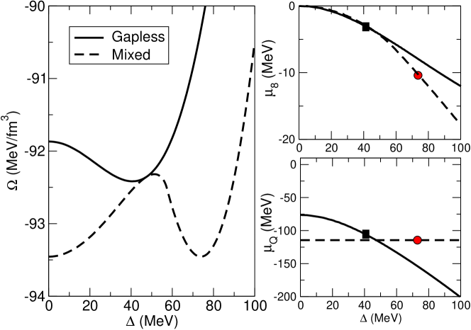
Figure 1: In the left panel, free energy curves for the gapless (solid) and the mixed phases (dashed) as a function of $\Delta$ for $\mu=350$ MeV are shown. The gapless free energy is characterized by the imposition of local electric and color charge neutrality while in the mixed phase electric charge neutrality is imposed globally. These requirements induce chemical potentials $\mu_{Q}$ and $\mu_{8}$ and are shown in the right panels. The filled dots and rectangles indicate the locations of the mixed and the gapless ground states.

Bulk matter is neutral with respect to electric and color charge. In what follows we investigate both the homogeneous and the heterogeneous phases. For the former, electric and color charge neutrality is a local condition. In this case, for a given baryon chemical potential $\mu$, we require that

$$-\frac{\partial\Omega_{\mathrm{2SC}}}{\partial\mu_{Q}}=0,\quad-\frac{\partial\Omega_{\mathrm{2SC}}}{\partial\mu_{3}}=0=-\frac{\partial\Omega_{\mathrm{2SC}}}{\partial\mu_{8}}\,.$$ (26)

These sets of equations determine $\mu_{Q}$, $\mu_{3}$, $\mu_{8}$ at any value of the gap $\Delta$. Simultaneously solving the above set of equations together with the gap equation $\partial\Omega_{\mathrm{2SC}}/\partial\Delta=0$ determines the gapless states. Denoting the solutions as $\tilde{\mu}_{Q}$, $\tilde{\mu}_{3}$, $\tilde{\mu}_{8}$ and $\tilde{\Delta}$, the free energy of the gapless phase is

$$\Omega_{\mathrm{gapless}}(\mu)\equiv\Omega_{\mathrm{2SC}}(\mu,\tilde{\mu}_{Q},\tilde{\mu}_{3},\tilde{\mu}_{8},\tilde{\Delta})\,.$$ (27)

To construct the mixed phase comprising of normal and superconducting states, electric charge neutrality is imposed as a global constraint. In principle we could have imposed color neutrality as a global constraint in the heterogeneous phase. However, we expect the color Debye screening length, $\lambda_{\mathrm{Debye-color}}\simeq 1/\mu$, to be short and comparable to the inter-particle distance in strong coupling. Under these conditions, color neutrality is essentially a local constraint. For normal and superconducting phases to co-exist they must satisfy the Gibbs criteria: for a given $\mu$, it requires equality of pressures at equal electric chemical potential. This results in the following condition

$$\Omega_{\mathrm{2SC}}(\Delta=0,\overline{\mu}_{Q})=\Omega_{\mathrm{2SC}}(\Delta_{\mathrm{BCS}},\overline{\mu}_{Q})\,,$$ (28)

which in turn uniquely determines $\overline{\mu}_{Q}$ corresponding to the mixed phase. Global charge neutrality follows as long as the normal and superconducting phases have opposite electric charge. The volume fraction of the superconducting phase, which we call $\chi$ is determined by the global constraint

$$\chi~{}Q_{\mathrm{SF}}+(1-\chi)~{}Q_{\mathrm{Normal}}= 0,$$ (29)

$$\mathrm{where}\quad Q_{\mathrm{SF}}=-\frac{\partial\Omega_{\mathrm{2SC}}(\Delta_{\mathrm{BCS}},\mu_{Q})}{\partial\mu_{Q}}\Big{|}_{\overline{\mu}_{Q}}, \ \ Q_{\mathrm{Normal}}=-\frac{\partial\Omega_{\mathrm{2SC}}(\Delta=0,\mu_{Q})}{\partial\mu_{Q}}\Big{|}_{\overline{\mu}_{Q}},$$

are the electric charge densities of the superconducting and normal phases respectively.

In Fig. 1, we show the free energy $\Omega_{\mathrm{2SC}}$ as a function of $\Delta$ for $\mu=350$ MeV. The solid curve is for the case where electric and color charge neutrality conditions are imposed locally. The minimum seen at $\Delta\simeq 40$ MeV corresponds to the gapless superconducting state described earlier. The dashed curve shows the free energy corresponding to the mixed phase. Here we have imposed only local color neutrality and determined the electric chemical potential using Eq. (28). Accordingly, it shows the existence of two degenerate minima corresponding to the normal and BCS superconducting states. The variation of the electric and color chemical potentials are also shown in Fig. 1. We find that $\tilde{\mu}_{3}=0$ and $|\tilde{\mu}_{8}|\ll|\overline{\mu}_{Q}|<|\mu_{B}|$. The electric charge chemical potential in the mixed phase is large. For our choice of model parameters and for $\mu$ in the interval $300-500$ MeV we find that the ratio $\Delta_{0}/\delta\mu\simeq 1.3$. This is consistent with, but smaller than, the weak-coupling leading order prediction of $\Delta_{0}/\delta\mu=\sqrt{2}$. On the other hand, $\tilde{\mu}_{8}$ is small and proportional to $\Delta_{0}^{2}/\mu$ since it is only through pairing that color neutrality is upset.

III Coulomb and Surface Energy in the Mixed Phase

The mixed phase free energy in Fig. 1 ignores finite size contributions arising due to Coulomb and surface energies associated with phase separation. If these effects are negligible, the results clearly indicate that the mixed phase is favored over the gapless phase. However, given the small difference in free energy between the gapless and mixed phases including these corrections becomes necessary. In Sec. IV we calculate the surface energy in the mixed phase. For now, we treat the surface tension as a parameter and study how it influences the free energy of the mixed phase.

The mixed phase can be subdivided into electrically neutral unit cells called Wigner-Seitz cells, as in the analysis of the inner crust of a neutron star where droplets of charged nuclear matter coexist with a negatively charged fluid of neutrons and electrons Negele:1973vb . In the present context, each Wigner-Seitz cell will contain some positively charged superconducting quark matter and some negatively charged normal quark matter. Although at low temperature these unit cells form a Coulomb lattice, the interaction between adjacent cells can be neglected compared to the surface and Coulomb energy of each cell. In this Wigner-Seitz approximation, the surface and Coulomb energy per unit volume are fairly straightforward to calculate if the charge density is spatially uniform in each phase and if the surface thickness is small compared to the spatial extent of the Wigner-Seitz cell. We will examine both these requirements in greater detail in Sec. IV. For now we shall assume that these requirements are satisfied. In this case, the surface and Coulomb energies depend in general on the geometry and are given by Ravenhall:1983uh

$$E^{S} = \frac{d~{}x~{}\sigma}{r_{0}}\,,$$ (30)

$$E^{C} = 2\pi~{}\alpha_{\rm em}f_{d}(x)~{}x~{}(\Delta Q)^{2}~{}r_{0}^{2}\,,$$ (31)

where $d$ is the dimensionality of the structure ($d=1,2,$ and $3$ correspond to Wigner-Seitz cells describing slab, rod and droplet configurations, respectively), $\sigma$ is the surface tension, $\Delta Q=Q_{\rm SF}-Q_{\rm Normal}$ is the charge density contrast between the two phases and $\alpha_{\rm em}=1/137$ is the fine structure constant. The other factors appearing in Eqs. (30) and (31) are: $x$, the fraction of the rarer phase which is equal to $\chi$ for $\chi\leqslant 0.5$ and $1-\chi$ for $0.5<\chi\leqslant 1$; $r_{0}$, the radius of the rarer phase (radius of drops or rods and half-thickness of slabs); and $f_{d}(x)$, the geometrical factor that arises in the calculation of the Coulomb energy which can be written as

$$f_{d}(x)=\frac{1}{d+2}~{}\left(\frac{2-d~{}x^{1-2/d}}{d-2}+x\right)\ .$$ (32)

The first step in the calculation is to evaluate $r_{0}$ by minimizing the sum of $E^{C}$ and $E^{S}$. The result is

$$r_{0}=\left[\frac{d~{}\sigma}{4\pi~{}\alpha_{\rm em}f_{d}(x)~{}(\Delta Q)^{2}}\right]^{1/3}\,.$$ (33)

We then use this value of $r_{0}$ in Eqs. (30) and (31) to evaluate the surface and Coulomb energy cost per unit volume

$$E^{S}+E^{C}=\frac{3}{2}\left(4\pi~{}\alpha_{em}~{}d^{2}~{}f_{d}(x)~{}x^{2}\right)^{1/3}~{}(\Delta Q)^{2/3}~{}\sigma^{2/3}\,.$$ (34)

This equation allows us to include the free energy cost associated with the Coulomb field and the surface. After calculating the surface tension in Sec. IV we will return to an analysis of the free energy competition between gapless and mixed phases in Sec. V.

IV Surface Tension

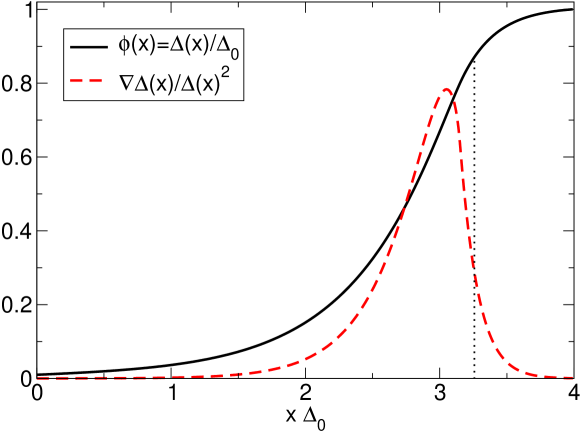
Figure 2: The profile of $\Delta(x)$ at the interface for $\mu=400$ MeV. The solid curve shows the variation of the dimensionless quantity $\phi(x)=\Delta(x)/\Delta_{0}$ as function of the $\bar{x}=x\Delta_{0}$. The dotted-line corresponds to the region where the leading order gradient energy is less than zero when $\delta\mu$ corrections from Ref. Huang:2004bg are included. The dashed curve shows the variation of $\nabla\Delta(x)/\Delta(x)^{2}$.

We will now calculate the surface energy associated with the normal-superconductor interface. This will allow us to determine if the mixed phase is favored over the gapless state. To accomplish this we will need to allow for spatial variations of $\Delta$ and calculate the gradient contribution to the free energy. Near the critical temperature one can employ Landau-Ginsburg theory to obtain the leading gradient contribution to the free energy. In this case, the gradient expansion (in powers of $|\nabla~{}\Delta(x)|^{2}$) is well defined. Bailin and Love have derived an expression for the gradient contribution to the free energy for a relativistic superconductor near the critical temperature Bailin:1984bm . In the context of dense quark matter, a discussion of the Landau-Ginsburg theory for two and three flavor quark matter can be found in Refs. Iida:2000ha ; Voskresensky:2004jp . For temperatures that are small compared to the critical temperature, the gradient expansion (in powers of $|\nabla~{}\Delta(x)|^{2}$) has poor convergence properties and one must in principle include gradients to all orders. However, if the spatial variations of $\Delta$ occur on a length scale that is numerically large compared to $\Delta^{-1}$, it is a good approximation to retain only the leading term. We shall assume that the thickness of the normal-superconductor interface is larger than $\Delta^{-1}$ and retain only the leading contribution from the gradient term. In this case, the $\Delta$ dependent contribution to the free energy of the 2SC phase, including the gradient term, is given by

$$\mathcal{F}(\Delta)_{\mathrm{2SC}}= \Omega_{\mathrm{2SC}}+\kappa_{\mathrm{2SC}}^{(2)}|\nabla~{}\Delta(x)|^{2}+{\mathrm{O}}(|\nabla~{}\Delta(x)|^{4}/\Delta^{4})\,.$$ (35)

The coefficient of the gradient term ($\kappa_{\mathrm{2SC}}$) for the 2SC phase, which is related to the Meissner mass of the gluons, at zero temperature and for the case where $\delta\mu=0$ has been calculated in earlier work by Rischke Rischke:2000qz . Recently, Huang and Shovkovy have investigated how $\delta\mu$ affects the Meissner masses (which as discussed earlier, in turn determines $\kappa_{\mathrm{2SC}}$) Huang:2004bg . They find that the Meissner mass of the eight gluon (assuming that the condensate aligns in the 3 direction) remains unaffected by $\delta\mu$ in the BCS phase i.e, for $\delta\mu\leq\Delta_{0}$. On the other hand, they find the Meissner masses of gluons with color 4,5,6,7 (which are degenerate) decrease with increasing $\delta\mu$ and become negative when $\delta\mu=\Delta_{0}/\sqrt{2}$. Surprisingly, these gluon masses become negative even in the BCS phase, i.e, for $\Delta_{0}/\sqrt{2}\leq\delta\mu\leq\Delta_{0}$ . It is presently not clear how this instability is resolved. In this work, where we have employed an Nambu-Jona-Lasino (NJL) model description of the interaction between quarks, the gluons are introduced as fictitious gauge fields solely for the purpose of determining the coefficient $\kappa_{\mathrm{2SC}}$ in the effective theory for the real field $\Delta$ Son:1999cm . By minimal coupling between the field $\Delta$ and the gluons, the relation between $\kappa_{\mathrm{2SC}}$ and the Meissner mass ($m_{g}^{2}~{}\simeq~{}\alpha_{s}^{2}\mu^{2}$) of the gluons is obtained by matching to be $\kappa_{\mathrm{2SC}}^{(2)}\propto m_{g}^{2}/\alpha_{s}^{2}\Delta_{0}^{2}$, where $\alpha_{s}$ is the strong coupling constant.

In our calculation, the coefficient $\kappa_{\mathrm{2SC}}^{(2)}$ is determined by matching the mass of the fourth and eight gluon in the effective theory to the microscopic calculation. We note that $\kappa_{\mathrm{2SC}}^{(2)}$ could depend on $\Delta(x)$, since the low energy effective theory for the real field $\Delta(x)$ does not have a well defined expansion parameter. Hence, in general

$$\kappa_{\mathrm{2SC}}^{(2)}=\sum_{n=0,\infty}~{}a_{n}~{}\left(\frac{\Delta(x)}{\Delta_{0}}\right)^{2n}\,,$$ (36)

where $a_{n}$ are constants that remain to be determined by matching conditions. We make the simplifying assumption made in Ref. Rischke:2000qz and retain only the leading ($a_{0}$) and next to leading ($a_{1}$) order terms. In this case, using the Meissner masses calculated in Ref. Huang:2004bg and for $\Delta_{0}\geq\delta\mu$ we obtain

$$\kappa_{\mathrm{2SC}}^{(2)}=\frac{\bar{\mu}^{2}}{3\pi^{2}~{}\Delta_{0}^{2}}~{}\left[(1-2\frac{\delta\mu^{2}}{\Delta_{0}^{2}})-\frac{1}{2}~{}(1-4\frac{\delta\mu^{2}}{\Delta_{0}^{2}})\frac{\Delta(x)^{2}}{\Delta_{0}^{2}}\right]\,,$$ (37)

where $\bar{\mu}=\mu+\mu_{Q}/6+\mu_{8}$ is the common chemical potential of the quarks participating in pairing and $\delta\mu=\mu_{Q}/2$. From Eq. 37 we see that for $\Delta_{0}/\delta\mu\leq\sqrt{2}$, the coefficient $a_{0}\leq 0$ while $a_{1}$ remains positive in the mixed phase where $\Delta_{0}/\delta\mu\geq 1$. In weak coupling and to leading order in the $\Delta_{0}$ and $\delta\mu$, the mixed phase occurs precisely at $\Delta_{0}/\delta\mu=\sqrt{2}$. In our calculation of the mixed phase free energy in Sec. II we found that $\Delta_{0}/\delta\mu\simeq 1.3$ for $\mu$ in the interval $300-500$ MeV. This result, which implies that $\Delta_{0}/\delta\mu<\sqrt{2}$ is not generic to the mixed phase. For other values of the coupling we indeed find that $\Delta_{0}/\delta\mu\geq\sqrt{2}$ and both $a_{0}$ and $a_{1}$ are positive. Nonetheless, even when $a_{0}\leq 0$, for $\Delta(x)/\Delta_{0}\simeq 1$, the $a_{1}$ term ensures that the gradient contribution is positive and is therefore crucial for the stability of the BCS phase component of the mixed phase. In the vicinity of the BCS phase, i.e, when $\Delta(x)/\Delta_{0}\simeq 1$, the gradient contribution is independent of $\delta\mu$ and $\kappa_{\mathrm{2SC}}^{(2)}=\bar{\mu}^{2}/6\pi^{2}\Delta_{0}^{2}$. We note that had we retained only the $a_{0}$ contribution to $\kappa_{\mathrm{2SC}}^{(2)}$ and matched to the mass of the eight-gluon (arguing that in our NJL model treatment only the generators $T_{3}$ and $T_{8}$ are relevant) we would still have obtained $\kappa_{\mathrm{2SC}}^{(2)}=\bar{\mu}^{2}/6\pi^{2}\Delta_{0}^{2}$. A non-zero $\delta\mu$ in general acts to reduce the energy cost associated with the gradient term when $\Delta(x)/\Delta_{0}$ decreases from unity. Surprisingly, when $\Delta(x)/\Delta_{0}=\sqrt{2(2(\delta\mu^{2}/\Delta_{0}^{2})-1)/(4(\delta\mu^{2}/\Delta_{0}^{2})-1)}$, the gradient energy goes to zero. This does not necessarily mean that the interface is unstable since we have not investigated the higher order gradient terms. However, this trend suggests that we can obtain an upper bound on the surface tension by using the (largest) value of $\kappa_{\mathrm{2SC}}^{(2)}=\bar{\mu}^{2}/6\pi^{2}\Delta_{0}^{2}$ across the whole interface. We note in passing that for temperatures near $T_{C}$, where $T_{C}$ is the BCS critical temperature, Bailin and Love Bailin:1984bm find that

$$\kappa_{\mathrm{2SC}}^{(2)}=\frac{7\zeta(3)}{24\pi^{4}}~{}\frac{\mu^{2}}{\alpha^{2}~{}\Delta_{0}^{2}}\,$$ (38)

where $\alpha\simeq 0.57=k_{B}T_{C}/\Delta_{0}$, $\zeta(3)\simeq 1.202$. Interestingly, the results for $\kappa_{\mathrm{2SC}}^{(2)}$ in the vicinity of the BCS state at $T=0$ and $T\sim T_{C}$ are both parametrically and numerically similar.

The contribution to the free energy which is independent of spatial derivatives is given by $\Omega_{\mathrm{2SC}}(\Delta)$ and was derived earlier in Eq. (25). In general, both the gradient term and $\Omega_{\mathrm{2SC}}$ are functions of all three chemical potentials, namely: $\mu$, $\mu_{Q}$ and $\mu_{8}$. While we retain this full dependence in $\Omega_{\mathrm{2SC}}$ we use the approximate form for $\kappa_{\mathrm{2SC}}^{(2)}$ valid when $\Delta(x)\simeq\Delta_{0}$. To construct the spatial profile of $\Delta$ between the normal and superconducting phases we use the equation of motion. In one spatial dimension this is given by

$$\kappa_{\mathrm{2SC}}\frac{d^{2}\Delta(x)}{dx^{2}}+(\frac{d\Delta(x)}{dx})^{2}\frac{\partial\kappa_{\mathrm{2SC}}}{\partial\Delta}=\frac{\partial\Omega_{\mathrm{2SC}}}{\partial\Delta}\,.$$ (39)

We solve this ordinary differential equation subject to the boundary condition that $\Delta(x=0)=0$ and $\Delta(x)=\Delta_{0}(\mu)$ at large $x$, where $\Delta_{0}(\mu)$ is the gap in the BCS phase. The results are shown in Fig. 2, where we calculate the interface for various values of the baryon chemical potential $\mu=400$ MeV. We find that the profiles for the interface for other values of $\mu$ in the range $350-450$ MeV show nearly identical behavior when plotted in terms of the reduced dimensionless units $\phi(x)=\Delta(x)/\Delta_{0}(\mu)$ and $\bar{x}=x\Delta_{0}(\mu)$. The typical length scale for the variation of $\Delta$ is parametrically similar to but numerically larger than $\Delta_{0}^{-1}$. We find that a rough measure of the thickness $t\simeq(1.5-2)\Delta_{0}^{-1}$. As mentioned earlier, due to the lack of a well defined gradient expansion for effective theory at $T=0$, the validity of the leading order (in the gradient expansion) results requires that the spatial variation of $\Delta(x)$ be weak and satisfy the condition $\nabla\Delta/\Delta_{0}^{2}\ll 1$. From Fig. 2, we see that this condition is satisfied to a fair degree (see dashed lines). Using these profiles, we have computed the surface tension by integrating the free energy function given in Eq. (35). The results are presented in the table below.

$\mu$ (MeV)	$\sigma$ (MeV/fm2)	$\mu$ (MeV)	$\sigma$ (MeV/fm2)	$\mu$ (MeV)	$\sigma$ (MeV/fm2)
350	1.9	375	2.6	400	3.6
425	4.9	450	6.8	475	9.4

Our estimation of the coefficient of the kinetic term, which we call $\kappa_{\mathrm{2SC}}^{(2)}$ ignores several possible corrections. Including those due to the truncation of the series in Eq. 36, and the neglect of $\delta\mu$. As discussed earlier the effect of $\delta\mu$ is to decrease the gradient contribution, consequently we can expect these corrections to lower our estimate of the surface tension. In Fig. 2, the vertical dotted-line indicates the region where the gradient energy is less than zero when $\delta\mu$ corrections are included. In this case, the profile would resemble the dotted-line rather than the solid line and corresponding surface energy is greatly reduced. We have also examined how an increase in $\kappa_{\mathrm{2SC}}^{(2)}$ would affect our calculation of the surface tension. We find that these changes are modest. The surface tension $\sigma$ increased by $40\%$ when $\kappa_{\mathrm{2SC}}$ was increased by a factor of two.

V Phase Diagram

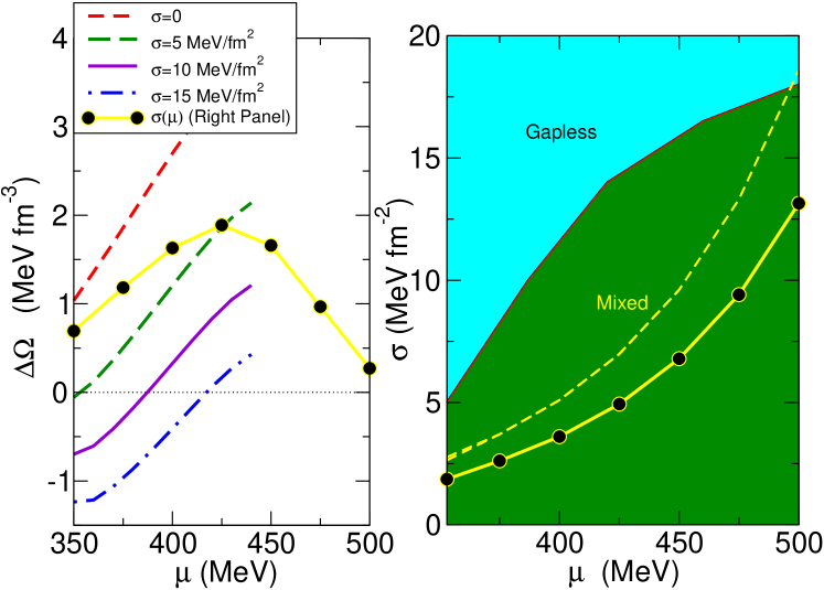
Figure 3: Left panel: Influence of the surface energy on the total free energy difference between the gapless and the mixed phases $\Delta\Omega=\Omega_{\mathrm{gapless}}-\Omega_{\mathrm{mixed}}$ for various values of the surface tension. The filled circles correspond to values of $\sigma(\mu)$ shown in the right panel. Right panel: The phase diagram showing the favored phase as a function of the surface tension and baryon chemical potential. The filled circles correspond to the results obtained from calculation of the surface tension outlined in Sec. IV. The dashed line shows the surface tension when $\kappa_{\mathrm{2SC}}^{(2)}$ was increased by a factor of two.

Using the results of the previous sections, we can study the free energy competition between the gapless and the mixed phases. The free energy of the mixed phase, including Coulomb and surface contributions is

$$\Omega_{\mathrm{mixed}}(\mu)=\Omega_{\mathrm{2SC}}(\mu,\overline{\mu}_{Q})+E^{S}+E^{C}\,,$$ (40)

where the surface and the Coulomb contributions were defined in Eq. (34) and $\overline{\mu}_{Q}$ is defined through Eq. (28). The left panel of the Fig. 3 shows the free energy difference $\Delta\Omega=\Omega_{\mathrm{gapless}}-\Omega_{\mathrm{mixed}}$ for various values of the surface tension in the mixed phase. The filled circles correspond to the values of the surface tension computed in Sec. IV. We have used this information in constructing the ”phase diagram” as a function of $\mu$ and $\sigma$, and is shown in the right panel of the figure. As expected, the gapless homogeneous phase is favored when $\sigma$ is large and the mixed phase is favored for small $\sigma$. The surface tension computed in the previous section is also shown (filled circles). Their low values at small $\mu$ indicate that the mixed phase is favored at low density. At first, with increasing density the free energy difference ($\Delta\Omega$) increases, resulting in a robust mixed phase. For $\mu\,\raisebox{-3.44444pt}{$\stackrel{{\scriptstyle\textstyle>}}{{\sim}}$ }450$ MeV the free energy difference decreases, indicating a possible first-order transition to the gapless phase at high density. The dashed dashed-curve on the right panel shows the surface tension for the case where we artificially increased $\kappa_{\mathrm{2SC}}^{(2)}$ by a factor of two. In this case the trends are similar, the mixed phase continues to be favored at low density and a first order transition to the gapless phase occurs at $\mu\simeq 500$ MeV. To eliminate the mixed phase $\kappa_{\mathrm{2SC}}^{(2)}$ has to be at least on order of magnitude larger than the one used in this work.

We now examine if the assumptions made earlier in constructing the mixed phase are satisfied for the values of the surface tension calculated in Sec. IV. The Debye screening length in the normal and superconducting phases are easily computed by using the relation $\lambda_{D}^{-2}=-4\pi~{}\alpha_{\mathrm{em}}~{}\partial^{2}\Omega_{\mathrm{2SC}}/\partial\mu_{Q}^{2}$. For the individual phases to have uniform charge distributions, their spatial extents in the mixed phase must be small compared to the Debye screening length. The table below provides a comparison between these length scales at various values of the baryon chemical potential. The results are shown for the mixed phase with $d=3$, corresponding to a spherical geometry for the Wigner-Seitz. In the table, $\Delta_{\mathrm{BCS}}$, $\chi$, $R_{\mathrm{D}}$ and $R_{\mathrm{ws}}$ correspond to the gap in the BCS phase, the volume fraction of the BCS phase, the droplet radius and the radius of the Wigner-Seitz cell respectively. Further, we have also implicitly assumed that the interface thickness is small compared to $R_{\mathrm{D}}$ and $R_{\mathrm{ws}}$. The thickness parameter $t$, defined to be the distance over which the gap roughly decreases by a factor of $e\simeq 2.718$, is also given in the table.

$\mu$ (MeV)	$\Delta_{\mathrm{BCS}}$ (MeV)	$\chi$	$R_{\mathrm{D}}$ (fm)	$R_{\mathrm{ws}}$ (fm)	$\lambda_{D}^{\mathrm{sc}}$ (fm)	$\lambda_{D}^{\mathrm{normal}}$ (fm)	$t$ (fm)
350	74	0.4	6	8	7	5	4
400	106	0.7	4	6	6	4.5	3
450	140	0.8	3	5	5	4	2
500	174	0.9	3	5	5	4	2

The length scales shown in the above table are just barely compatible with our earlier assumptions. In particular, the Debye screening length and the spatial extents are of similar size, the charge distribution in the mixed phase could differ from the simple profiles considered here. We also note that the thickness is not small compared to the typical size of the droplet or the Wigner-Seitz cell. We will not consider these finite size corrections in this work. These corrections generically tend to decrease the Coulomb energy, increase the surface energy and penalize the mixed phase when the volume fraction $\chi$ is near zero or unity Norsen:2000wb ; Voskresensky:2002hu . These finite size effects in the mixed phase clearly warrant further study.

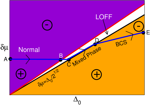
Figure 4: A schematic phase diagram at mixed $\mu$. The BCS gap $\Delta_{0}$ (or equivalently the effective four-fermion coupling constant) is plotted along the x-axis and $\delta\mu=\mu_{Q}/2$ is the y-axis. The line $\delta\mu=\Delta_{0}/\sqrt{2}$ separates the regions where the BCS state (lower-right) and the normal states (upper-left) are favored. The charge-neutral ground state follows the trajectory shown by the thick lines with arrows. The wedged region between the lines corresponding to $\delta\mu=\Delta_{0}/\sqrt{2}$ and $\delta\mu=0.75\Delta_{0}$ indicates the region were the LOFF phase may be favoredAlford:2000ze .

The results of this work combined with the finding of earlier investigations in Refs. Alford:2000ze ; Alford:2002kj ; Steiner:2002gx ; Neumann:2002jm of the charge neutral two flavor quark matter suggest a schematic phase diagram of the form shown in Fig. 4. The figure depicts the phase structure at fixed $\mu$ . The BCS gap $\Delta_{0}$ or equivalently the effective four-fermion coupling increases along the x-axis and $\delta\mu=\mu_{Q}/2$ increases along the y-axis. The line $\delta\mu=\Delta/\sqrt{2}$ separates the regions where the BCS state (lower-right) and the normal states (upper-left) are favored (As discussed earlier, this is true only in weak coupling. In strong coupling, $\delta\mu$ lies in the vicinity of $\Delta_{0}/\sqrt{2}$). The charge-neutral ground state follows the trajectory shown by the thick lines with arrows. In each phase, regions above this line correspond to net positive charge and regions below to net negative charge. For small coupling ($\Delta_{0}$), the homogeneous normal phase is preferred, and is represented by the line from point A to B. At intermediate coupling, the mixed phase containing an admixture of negatively charged normal phase coexisting with positively charged BCS phase is favored. This is shown by the line from point C to D. At large coupling, the homogenous BCS or 2SC phase prevails and is depicted by the line from point D to E. The wedged region between the lines corresponding to $\delta\mu=\Delta/\sqrt{2}$ and $\delta\mu=0.75\Delta$ indicates the region were the LOFF phase may be favoredAlford:2000ze . It remains to be seen how this phase could exist as a charge-neutral state. If the charge density in the LOFF phase resembles the normal phase, the figure supports the existence of a region between point B and C where the LOFF phase could be stable and electrically neutral. It also points to the possibility of a mixed phase of LOFF and BCS. Investigation of the LOFF phase in the charge neutral phase diagram is clearly warranted but is beyond the scope of this article.

VI Discussion

Based on our calculation of the surface tension between normal and superconducting 2-flavor quark matter we have shown that a heterogeneous mixed phase is likely to be the ground state of quark matter at low density. The stress induced on the bulk system by the requirement of charge neutrality is resolved by phase separation. The other possibility, which is the homogeneous gapless phase is energetically disfavored at low density. As depicted in Fig. 4, at small coupling we can expect the charge neutral ground state to be be in the normal phase. At intermediate coupling, the heterogeneous mixed phase is favored and large coupling a uniform BCS like 2SC phase is the ground state.

While we expect our qualitative results to be fairly robust, there are three important caveats to our quantitative findings that we shall now discuss. First of these caveats is related to the earlier observation that the surface thickness $t\simeq 1-3$ fm, the typical physical sizes of the charged regions $R_{\mathrm{D}}\simeq=2-6$ fm and the Debye screening length $\lambda_{D}\simeq 5-8$ fm are not well separated. This is likely to alter the simple structure of the mixed phase considered in this work. The charge, baryon density and the gap will vary smoothly over most of the Wigner-Seitz cell. These finite size corrections will need to be examined before one can draw firm conclusions regarding the phase competition (for a discussion of these effects in the context of a nuclear-kaon mixed phase see Ref. Norsen:2000wb ). Second, we have assumed that the weak coupling BCS theory holds even when $\Delta/\mu\simeq 1/3$. In the BCS limit $\Delta\ll\mu$, neither the gapless nor the mixed phase could exist because for 2-flavor quark matter the electric charge chemical potential is proportional to the baryon chemical potential. In the strong coupling regime it is difficult to know a priori how other contributions to the free energy would alter this competition. Finally, we have only included the leading order gradient contribution in the effective theory for $\Delta$. Although our profiles indicate that spatial variation of $\Delta(x)$ is mild (From Fig. 2, $|\nabla\Delta(x)|^{2}/\Delta_{0}^{2}\,\,\raisebox{-3.44444pt}{$\stackrel{{\scriptstyle\textstyle<}}{{\sim}}$ }1$), it is a priori not possible to assess how the higher order spatial derivatives of $\Delta(x)$ in the free energy would change our estimate of the surface tension. As could corrections to the coefficient $\kappa_{\mathrm{2SC}}^{(2)}$ arising from strong coupling and the lack of well defined expansion parameter for the effective theory at $T=0$. Additionally, corrections due to electric and color charge chemical potentials are important Huang:2004bg . Interestingly, the correction to the gradient term from the electric charge chemical potentials tends to decrease the surface energy. We have shown that drastic changes to $\kappa_{\mathrm{2SC}}^{(2)}$ (an increase by a factor of 2) resulted in a surface tension that continued to favor the mixed phase at low density. In this case, with increasing density, we found that the gapless phase becomes favored. The location of this first order transition between the mixed phase and the gapless phase is model dependent since it is sensitive to the density dependence of the ratio $\mu/\Delta_{0}$.

An important consequence of $\delta\mu$ corrections to the kinetic term concerns stability of the gapless phase. First we note that we can expect the matching between the kinetic coefficients for the effective theory for $\Delta(x)$ and the masses of gluons in the microscopic theory to be valid in the gapless phase. Since $\delta\mu\geq\Delta_{0}$ in the gapless phase this implies an instability of the spatially uniform gapless phase (the leading order gradient energy is negative). How this instability is resolved is not clear at this time. It is however clear that some type of heterogeneity must occur. Likely candidate states include the LOFF phase and the mixed phase. Pending a detailed investigation of the charge neutral LOFF state, our results suggest that this instability may be resolved by the formation of a mixed phase. In our NJL model study, the mixed phase is stable with respect to small gradient perturbations for all $\Delta_{0}/\delta\mu\geq 1$. In weak coupling, since $\Delta_{0}/\delta\mu=\sqrt{2}$ in the mixed phase, the chromo-magnetic instability discussed in Ref. Huang:2004bg for gluons 4-7 in QCD does not occur in the mixed phase. In strong coupling, whether this instability persists and if so, the nature of its resolution is not yet clear.

A heterogeneous quark matter ground state has important consequences for neutron star physics - were quark matter to exist inside their cores. The free energy difference between the gapless and mixed phase is small. Consequently, its effects on neutron star structure will be small. On the other hand, we can expect important changes to the transport properties induced by the heterogeneity of the mixed phase. In this phase, transport of the low energy neutrinos, photons, etc., will be dominated by coherent scattering induced by the presence of superconducting “bubbles” of quark matter with typical dimension of $r_{0}\simeq 5$ fm (for a discussion of how heterogeneity affects low energy neutrino transport see Ref. Reddy:1999ad ). Further, the existence of regions with normal quark matter will affect the neutrino emissivities - since they are typically large in the normal phase. Finally, the crystalline structure of the mixed phase could be relevant to the modeling of glitches observed in some pulsars.

We note that there are other mixed phases that could play a role in neutron stars. These include the mixed phase between quark matter and nuclear matterGlendenning:1992vb ; between color-flavor-locked matter and nuclear matterAlford:2001zr , or superconducting quark matter and normal quark matterNeumann:2002jm . All of these share several common features: the coexistence of positively and negatively charged phases separated by an interface; crystalline structure at low temperature; and coincidentally typical droplet sizes of the order $5$ fm. However, in these aforementioned examples it is still unclear if the mixed phase is favored when surface and Coulomb costs are included. This is because the surface tension is poorly known. Arguments based on naive dimensional analysis indicate that the surface energy cost may indeed be too large in these systems Heiselberg:1993dx ; Alford:2001zr . The exception could be the mixed phases of normal and superconducting quark matter considered in Ref. Neumann:2002jm . In this case, the surface tension is computable and the physical considerations are very similar to those studied in this work.

Although quantitative aspects of the analysis presented in this work pertains to asymmetrical relativistic superconductors, our finding provide some qualitative insight into the behavior of non-relativistic superfluid that can be realized in ultra cold fermionic-atom traps being developed in the laboratory. Although there is no Coulomb cost associated with the mixed phase in these systems, a surface energy cost must be overcome when the surface to volume ratio is not negligible. The methods described in Sec. IV apply in general to asymmetrical fermion systems and its relevance to laboratory experiments is currently under investigation.

Acknowledgments

We would like to thank Mark Alford, Paulo Bedaque, Heron Caldas, Joe Carlson, Krishna Rajagopal, Igor Shovkovy and Dam Son for useful discussions. This research was supported by the Dept. of Energy under contract W-7405-ENG-36.

References

- (1) B. C. Barrois, Nucl. Phys. B129, 390 (1977).
- (2) D. Bailin and A. Love, Phys. Rept. 107, 325 (1984).
- (3) M. G. Alford, K. Rajagopal and F. Wilczek, Phys. Lett. B422, 247 (1998), [hep-ph/9711395].
- (4) R. Rapp, T. Schafer, E. V. Shuryak and M. Velkovsky, Phys. Rev. Lett. 81, 53 (1998), [hep-ph/9711396].
- (5) M. G. Alford, K. Rajagopal and F. Wilczek, Nucl. Phys. B537, 443 (1999), [hep-ph/9804403].
- (6) P. F. Bedaque and T. Schafer, Nucl. Phys. A697, 802 (2002), [hep-ph/0105150].
- (7) D. B. Kaplan and S. Reddy, Phys. Rev. D65, 054042 (2002), [hep-ph/0107265].
- (8) M. Alford, C. Kouvaris and K. Rajagopal, hep-ph/0311286.
- (9) I. Shovkovy and M. Huang, Phys. Lett. B564, 205 (2003), [hep-ph/0302142].
- (10) G. Sarma, Phys. Chem. Solid 24, 1029 (1963).
- (11) M. G. Alford, J. Berges and K. Rajagopal, Phys. Rev. Lett. 84, 598 (2000), [hep-ph/9908235].
- (12) W. V. Liu and F. Wilczek, Phys. Rev. Lett. 90, 047002 (2003), [cond-mat/0208052].
- (13) P. F. Bedaque, Nucl. Phys. A697, 569 (2002), [hep-ph/9910247].
- (14) P. F. Bedaque, H. Caldas and G. Rupak, Phys. Rev. Lett. 91, 247002 (2003), [cond-mat/0306694].
- (15) M. G. Alford, J. A. Bowers and K. Rajagopal, Phys. Rev. D63, 074016 (2001), [hep-ph/0008208].
- (16) N. K. Glendenning, Phys. Rev. D46, 1274 (1992).
- (17) N. K. Glendenning and S. Pei, Phys. Rev. C52, 2250 (1995).
- (18) I. Shovkovy, M. Hanauske and M. Huang, Phys. Rev. D67, 103004 (2003), [hep-ph/0303027].
- (19) J. W. Negele and D. Vautherin, Nucl. Phys. A207, 298 (1973).
- (20) D. G. Ravenhall, C. J. Pethick and J. R. Wilson, Phys. Rev. Lett. 50, 2066 (1983).
- (21) M. Huang and I. A. Shovkovy, hep-ph/0407049.
- (22) K. Iida and G. Baym, Phys. Rev. D63, 074018 (2001), [hep-ph/0011229].
- (23) D. N. Voskresensky, Phys. Rev. C69, 065209 (2004).
- (24) D. H. Rischke, Phys. Rev. D62, 034007 (2000), [nucl-th/0001040].
- (25) D. T. Son and M. A. Stephanov, Phys. Rev. D61, 074012 (2000), [hep-ph/9910491].
- (26) T. Norsen and S. Reddy, Phys. Rev. C63, 065804 (2001), [nucl-th/0010075].
- (27) D. N. Voskresensky, M. Yasuhira and T. Tatsumi, Nucl. Phys. A723, 291 (2003), [nucl-th/0208067].
- (28) M. Alford and K. Rajagopal, JHEP 06, 031 (2002), [hep-ph/0204001].
- (29) A. W. Steiner, S. Reddy and M. Prakash, Phys. Rev. D66, 094007 (2002), [hep-ph/0205201].
- (30) S. Reddy, G. Bertsch and M. Prakash, Phys. Lett. B475, 1 (2000), [nucl-th/9909040].
- (31) M. G. Alford, K. Rajagopal, S. Reddy and F. Wilczek, Phys. Rev. D64, 074017 (2001), [hep-ph/0105009].
- (32) F. Neumann, M. Buballa and M. Oertel, Nucl. Phys. A714, 481 (2003), [hep-ph/0210078].
- (33) H. Heiselberg, C. J. Pethick and E. F. Staubo, Phys. Rev. Lett. 70, 1355 (1993).