WKB approximation for multi-channel barrier penetrability
Abstract
Using a method of local transmission matrix, we generalize the well-known WKB formula for a barrier penetrability to multi-channel systems. We compare the WKB penetrability with a solution of the coupled-channels equations, and show that the WKB formula works well at energies well below the lowest adiabatic barrier. We also discuss the eigen-channel approach to a multi-channel tunneling, which may improve the performance of the WKB formula near and above the barrier.
pacs:
PACS numbers: 03.65.Sq,03.65.Xp,24.10.Eq,25.70.JjI Introduction
The coupled-channels approach has been a standard method in describing atomic, molecular, and nuclear reactions involving internal degrees of freedom [1, 2, 3, 4, 5]. In nuclear physics, for instance, the coupled-channels method has been successfully applied to heavy-ion fusion reactions at energies around the Coulomb barrier in order to discuss the effect of couplings between the relative motion of the colliding nuclei and inelastic excitations in the target nucleus [1, 2, 3]. At these energies, the fusion reaction takes place by a quantum tunneling, and the coupled-channels calculations well account for the enhancement of the barrier penetrability due to the channel couplings.
A difficulty in the coupled-channels calculations, however, is that it is sometimes not so easy to obtain a numerically stable solution with a controlled accuracy. This is particularly the case in the presence of closed channels and/or when the coupling strength is strong in the classically forbidden region. Several methods have been proposed in order to stabilize the numerical solution [4, 6, 7, 8].
In this paper, instead of directly integrating the coupled-channels equations with the stabilization techniques, we solve them using the WKB approximation. To this end, we employ the method of local transmission matrix, which was originally developed by Brenig and Russ in order to stabilize numerical solutions of the coupled-channels equations [4]. We solve the equation for the local transmission matrix under the semi-classical assumption, and generalize the well-known WKB formula for a barrier penetrability for a single channel to coupled-channel systems. Since the penetrability is expressed in a compact form, the resultant WKB formula is entirely free from the problem of numerical instability. Moreover, the WKB method can be easily applied to systems with a large number of degrees of freedom, while obtaining a direct solution of the coupled-channels equations can be computationally demanding. Also, the WKB method is useful in gaining a physical intuition for the dynamics of multi-channel tunneling.
The paper is organized as follows. In Sec. II, we set up the coupled-channels equations and introduce the local transmission matrix. We derive the semi-classical expression for the local transmission matrix, and obtain the WKB formula for a multi-channel penetrability. We apply the WKB formula to a three-channel problem, and compare the penetrability with the numerical solutions of the coupled-channel equations. In Sec. III. we discuss the penetrability at energies near and above the barrier height. The WKB formula which we derive works when the multiple reflection of the classical path under the barrier can be neglected, that is, at energies well below the barrier. We show that the eigen-channel approach can provide good prescriptions at higher energies, where the primitive WKB formula breaks down. We summarize the paper in Sec. IV.
II Multi-channel WKB formula
Our aim in this paper is to derive the WKB formula for penetrability for a one dimensional potential barrier in the presence of channel couplings. We consider the following coupled-channels equations:
| (1) |
Here, is the mass of a particle, is the excitation energy for the -th channel, and is the total energy of the system. is the wave function matrix, where refers to the channel while specifies the incident channel. Notice that we express the wave functions in a matrix form by combining linearly independent solutions of the coupled-channels equations, being the dimension of the coupled equations. For the situation where the particle is incident on the barrier from the right hand side, the boundary conditions for are given by,
| (2) | |||||
| (3) |
where is the wave number for the -th channel. The inclusive penetrability is then obtained as,
| (4) |
Let us now introduce the local transmission matrix defined by [4]
| (5) |
where with . From Eqs. (2) and (3), the asymptotic form of reads,
| (6) | |||||
| (7) |
Here, we have used the fact as . It is easy to show that the local transmission matrix obeys the equation[4],
| (8) |
where
| (9) |
is the local reflection matrix[4].
The WKB approximation may be obtained by neglecting in Eq. (8) [9, 10], that is,
| (10) |
A similar equation has been derived by Van Dijk and Razavy [9, 10], but by using the method of variable reflection amplitude (see also Ref. [11]). Notice that the asymptotic form of the local reflection matrix is [4]
| (11) | |||||
| (12) |
Neglecting in Eq. (8) is thus equivalent to ignoring the reflection, that is reasonable in the semi-classical limit. This, in fact, corresponds to the lowest order of the Bremmer expansion [12, 13, 14, 15, 16], where the WKB formula is obtained by approximating a smooth potential with a series of sharp potential steps ***The local reflection matrix satisfies the equation [4]. One may solve this equation perturbatively assuming that remains small and finding the correction to Eq. (10)..
For a single channel problem, Eq. (10) can be easily integrated to yield
| (13) |
For a coupled-channels problem, however, care must be taken in the integration, since and do not commute to each other in general. We attempt to solve Eq. (10) by discretizing the coordinate with a mesh spacing of . Replacing the derivative term by a simple point difference formula, we obtain
| (14) | |||||
| (15) | |||||
| (16) |
to the lowest order of . Using , the first factor in Eq. (16) is transformed to be
| (17) |
Approximating , we finally obtain
| (18) |
Iterating this equation backward from , we obtain
| (19) |
Substituting this expression into Eq. (4) together with Eq. (6), the WKB approximation to the multi-channel penetrability reads
| (20) |
This is the main result in this paper. Notice that the factor does not appear in the WKB formula, Eq. (20). In practice, one can evaluate Eq. (20) by diagonalizing at each . This yields
| (21) |
where is the eigen-vector of the matrix with the eigen-value of , and . For a one dimensional problem, Eq. (20) is reduced to the familiar WKB formula,
| (22) |
where and are the inner and the outer turning points, respectively.
Let us now apply the WKB formula (20) to a three-level problem. We consider the following coupling potential:
| (23) |
with
| (24) | |||||
| (25) |
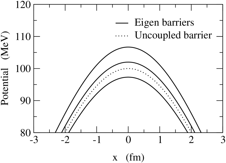
The parameters are chosen following Ref. [17] to be =100 MeV, =3 MeV, and 3 fm, which mimic the fusion reaction between two 58Ni nuclei. The excitation energy and the mass are taken to be 2 MeV and 29, respectively, where =938 MeV is the nucleon mass. With these parameters, the three eigen-barriers , which are obtained by diagonalizing at each , have the barrier height of 97.31, 102.0, and 106.7 MeV, respectively, while the barrier height for the uncoupled barrier is 100 MeV (See Fig.1).
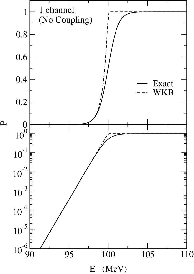
Before we study the three channel problem, let us first examine the validity of the WKB approximation for a single channel case to see whether the semi-classical approximation works in principle for the parameters which we choose. Figure 2 shows a comparison between the WKB penetrability for the uncoupled barrier (the dashed line) obtained with Eq. (20) and the exact solution. It is plotted in the linear and logarithmic scales in the upper and the lower panels, respectively. One clearly sees that the WKB approximation indeed works well at energies about 2 MeV below the barrier height and lower.
As it is well known, the naive WKB approximation breaks down around the barrier. In fact, the WKB penetrability is unity at the barrier height, while the exact result is about a half. Around these energies, one needs to improve the WKB formula by using the uniform approximation in order to take into account the multiple reflection of the classical path under the barrier [18, 19]. We will discuss this problem more in the next section in connection to the penetrability in a coupled-channels system.
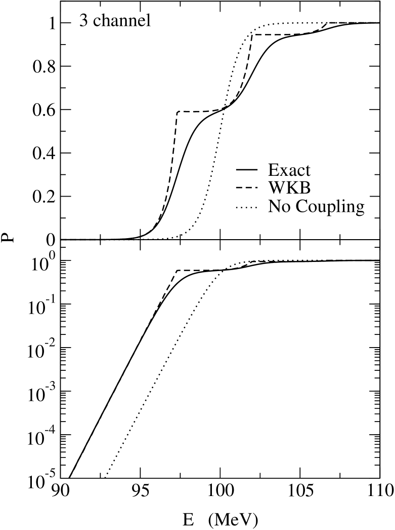
Let us now solve the coupled-channels problem, Eq. (23). We integrate Eq. (21) from fm to =15 fm with =0.05 fm. The dashed line in Fig. 3 shows the penetrability in the WKB approximation for this problem, which is compared to the exact solution of the coupled-channels equations (the solid line). The figure also shows the penetrability for the uncoupled barrier as a comparison (the dotted line). Remarkably, the WKB formula (20) reproduces almost perfectly the exact solution at energies well below the lowest adiabatic barrier, i.e., 97.31 MeV, as in the single channel problem.
We notice that the WKB penetrability increases much more rapidly than the exact penetrability at energies corresponding to the height of each eigenbarrier. This is in close analogue to the single channel problem shown in Fig. 2. This behaviour may be expected in the eigen-channel approach discussed in Refs. [17, 20, 21]. We will discuss this point in the next section.
III Penetrability near and above the barrier
In the previous section, we have shown that the multi-channel WKB formula works remarkably well at energies well below the lowest eigenbarrier. Therefore, it can be expected that the WKB formula provides a useful framework in discussing, for instance, the role of inelastic excitations in the colliding nuclei in nuclear reactions at extremely low energies, such as astrophysically relevant reactions, where the standard coupled-channels calculations may be difficult to carry out.
At higher energies, however, we found that the agreement between the primitive WKB formula and the exact solution of the coupled-channels equations becomes poor. For a single-channel problem, one can cure this problem by using the uniform approximation [18, 19]. The WKB formula which is valid at all energies is given by,
| (26) |
where the turning points and become complex numbers when the energy is above the barrier. It is not straightforward at all, however, to extend the uniform approximation to the coupled-channels problem. In this section, we instead present two prescriptions to deal with the coupled-channels penetrability at energies near and above the barrier.
A Dynamical Norm Method
The first prescription is closely related to the dynamical norm method developed in Ref. [22]. It was argued in Ref. [22] that the penetrability may be expressed as a product of the penetrability in the adiabatic limit and a multiplicative factor to it which accounts for the non-adiabatic effect. The latter factor, which was called the dynamical norm factor, was evaluated through the imaginary time evolution for an intrinsic degree of freedom with a classical path obtained with the adiabatic potential.
We follow here the same idea as in the dynamical norm method, and re-express Eq. (19) as
| (27) |
where is the local wave number for the lowest eigen-barrier (i.e., the adiabatic barrier), . The penetrability is then given by
| (28) |
The second factor on the right hand side (r.h.s.) of this equation is nothing more than the WKB penetrability for the adiabatic potential . At this stage, one may replace it by the exact penetrability for the adiabatic potential, . The first factor on the r.h.s. of Eq. (28) expresses the non-adiabatic effect, as in the dynamical norm factor introduced in Ref. [22]. Notice that our formula, (28), is in fact an improvement of the dynamical norm method in Ref. [22], since the classical path is not assumed from the beginning in evaluating the dynamical norm factor.
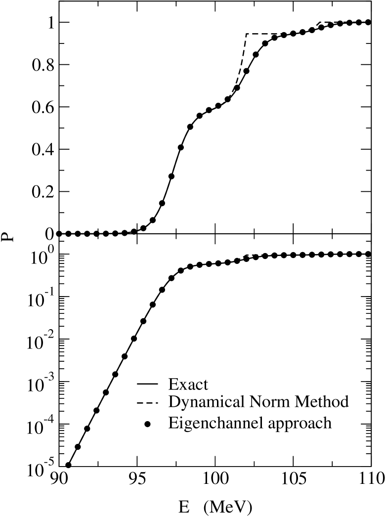
The result of the modified dynamical norm method is shown in Fig. 4 by the dashed line. It is evident that the agreement between the WKB approximation and the exact solution improves significantly at energies near and slightly above the adiabatic barrier, although the method provides essentially the same result as the original WKB formula, (20), at higher energies.
B Eigen-channel approach
The second prescription which we discuss is based on the eigen-channel approximation. In this approach, the penetrability is expressed as a weighted sum of the penetrability for the eigenbarriers [17, 20, 21], that is,
| (29) |
where is the penetrability for the eigen-potential . The weight factors are usually estimated by assuming that the matrix is independent of through the interaction range [17, 21], while the coordinate dependence of is properly taken into account in calculating the penetrability, . One often takes the barrier position of the uncoupled barrier, , in order to estimate the weight factors [21]. This leads to (see Eq.(21))
| (30) |
This procedure is indeed exact when the intrinsic degree of freedom has a degenerate spectrum [20, 23, 24, 25], since the matrix can be diagonalized independent of . When the intrinsic states have a finite excitation energy, however, the unitary matrix which diagonalizes explicitly depends on , and the results may depend strongly on the position where the weight factors are evaluated. Also the weight factors possess some energy dependence in general. In Ref. [20], we have explicitly shown for a two channel problem that the optimum weight factors are considerably different from those estimated at the barrier position, although their energy dependence appears to be weak. A satisfactory procedure to determine the weight factors has not yet been found so far when the excitation energy is finite.
In Fig.3, we have shown that the WKB penetrability approaches to a constant value at the barrier height of each eigen barrier. Assuming that the weight factors are independent of energy, one can exploit this fact to determine a consistent value of the weight factors in the eigen-channel approach. For instance, at the barrier height of the lowest eigenbarrier, , assuming that the contribution from the higher barriers is negligible, Eq. (29) suggests
| (31) |
in the primitive WKB approximation (i.e., without the uniform approximation). Therefore, if one evaluates Eq. (20) at , it directly provides the weight factor for the lowest eigenbarrier. One can repeat this procedure times to determine the weight factors : suppose that the weight factors for the lowest eigen-barriers have been determined. The weight factor for the -th eigenbarrier is then estimated as
| (32) |
where is the barrier height of the -th eigenbarrier, and is the penetrability in the WKB approximation, (20). Here, we have used the fact for in the primitive WKB approximation, and assumed for . The weight factor for the highest eigenbarrier is evaluated as
| (33) |
in order to ensure the unitarity.
We apply this prescription to the three channel problem discussed in the previous section. The weight factors are evaluated to be 0.5914, 0.3543, and 0.0543 for the lowest, the second lowest, and the highest eigen barriers, respectively. The result of the eigen channel approximation with the weight factors thus estimated is denoted by the filled circles in Fig. 4. The result is indistinguishable from the exact solution of the coupled-channels equations for all the energy region shown in the figure. We thus conclude that the multi-channel WKB formula which we derive in this paper provides a consistent way to determine the weight factors in the eigen-channel approach, and it provides a useful and simple prescription to compute the penetrability in the presence of channel couplings at energies from well below to well above the potential barrier, as long as the weight factors are slowly varying functions of energy.
IV Summary
We have extended the well known WKB formula for barrier penetrability to systems with intrinsic degrees of freedom. Applying the formula to a three channel problem, we have explicitly demonstrated that the WKB formula reproduces very nicely the exact solution of coupled-channels equations at energies well below the lowest eigenbarrier, i.e., the adiabatic barrier. The WKB formula which we derived is applicable even to systems with a large number of degrees of freedom, where the standard coupled-channels calculation cannot be performed due to a computational limitation. Our method may therefore provide a useful framework to discuss, e.g., a quantum scattering problem in the presence of coupling to a heat bath [26, 27]. The WKB formula is also useful when one discusses the channel coupling effect on the tunneling rate at deep subbarrier energies, especially in the presence of closed channels, since the direct integration of the coupled-channels equations may suffer from a numerical instability. Such interesting problems include heavy-ion fusion reactions at extremely low energies [28], electron screening effects in nuclear astrophysical reactions [29, 30], and nuclear structure effects in astrophysical fusion reactions [31, 32].
The WKB formula which we derived neglects the effect of multiple reflection of a classical path under the potential barrier. Such primitive formula breaks down at energies near and above the adiabatic barrier, as is well known. We discussed two prescription to cure this problem. One is the dynamical norm method, where the WKB formula is re-expressed as a product of the penetrability for the adiabatic barrier and a multiplicative factor which accounts for the non-adiabatic effect. By replacing the adiabatic penatrability in the WKB approximation by the exact one, we have shown that this prescription improves the result at energies near and slightly above the adiabatic barrier. The second prescription is the eigen-channel approximation, where the penetrability is given as a weighted sum of the eigen penetrability. By applying the WKB formula at energies corresponding to the barrier height of each eigen barrier, we have presented a consistent procedure to determine the weight factors. We have shown that this prescription works well at energies from well below to well above the barrier, as long as the energy dependence of the weight factors is negligible. This method would provide a useful way to simplify the coupled-channels calculations in realistic systems.
For a single channel problem, the primitive WKB formula can be improved by using the uniform approximation [18, 19], where the resultant WKB formula is applicable at energies both below and above the barrier. It will be an interesting, but very challenging, problem to extend it to a multi-channel problem. For this purpose, it will be extremely helpful to construct a solvable coupled-channels model. A work towards this direction is now in progress [33].
Acknowledgments
The authors thank H. Horiuchi and Y. Fujiwara for useful discussions. A.B.B. gratefully acknowledges the 21st Century for Center of Excellence Program “Center for Diversity and Universality” at Kyoto University for financial support and thanks the Yukawa Institute for Theoretical Physics for its hospitality. This work was supported in part by the U.S. National Science Foundation Grant No. PHY-0244384 and in part by the University of Wisconsin Research Committee with funds granted by the Wisconsin Alumni Research Foundation.
REFERENCES
- [1] A.B. Balantekin and N. Takigawa, Rev. Mod. Phys. 70, 77 (1998).
- [2] M. Dasgupta, D.J. Hinde, N. Rowley, and A.M. Stefanini, Annu. Rev. Nucl. Part. Sci. 48, 401 (1998).
- [3] K. Hagino, N. Rowley, and A.T. Kruppa, Comp. Phys. Comm. 123, 143 (1999).
- [4] W. Brenig, T. Brunner, A. Gross, and R. Russ, Z. Phys. B93, 91 (1993); W. Brenig and R. Russ, Surf. Sci. 315, 195 (1994).
- [5] N. Yamanaka and Y. Kino, Phys. Rev. A68, 052715 (2003).
- [6] B.R. Johnson, J. Chem. Phys. 69, 4678 (1978).
- [7] Z.H. Levine, Phys. Rev. A30, 1120 (1984).
- [8] T.N. Rescigno and A.E. Orel, Phys. Rev. A25, 2402 (1982).
- [9] W. Van Dijk and M. Razavy, Can. J. Phys. 57, 1952 (1979).
- [10] M. Razavy, Quantum Theory of Tunneling, (World Scientific Publishing Co., Singapore, 2003).
- [11] R. Bellman and R. Kalaba, Proc. Nat. Acad. Sci. U.S.A. 44, 317 (1958).
- [12] H. Bremmer, Physics 15, 593 (1949).
- [13] R. Landauer, Phys. Rev. 82, 80 (1951).
- [14] M.V. Berry, J. Phys. A15, 3693 (1982).
- [15] N.T. Maitra and E.J. Heller, Phys. Rev. A54, 4763 (1996).
- [16] S. Gasiorowicz, Quantum Physics (Wiley, New York, 1974).
- [17] C.H. Dasso, S. Landowne, and A. Winther, Nucl. Phys. A405, 381 (1983); A407, 221 (1983).
- [18] D.M. Brink and U. Smilansky, Nucl. Phys. A405, 301 (1983).
- [19] D.M. Brink, Semi-Classical Methods for Nucleus-Nucleus Scattering (Cambridge University Press, Cambridge, England, 1985).
- [20] K. Hagino, N. Takigawa, and A.B. Balantekin, Phys. Rev. C56, 2104 (1997).
- [21] C.H. Dasso and S. Landowne, Phys. Lett. B183, 141 (1987).
- [22] N. Takigawa, K. Hagino, and M. Abe, Phys. Rev. C51, 187 (1995).
- [23] K. Hagino, N. Takigawa, J.R. Bennett, and D.M. Brink, Phys. Rev. C51, 3190(1995).
- [24] M.A. Nagarajan, A.B. Balantekin, and N. Takigawa, Phys. Rev. C34, 894(1986).
- [25] H. Esbensen, Nucl. Phys. A352, 147(1981).
- [26] B. Barkakaty and S. Adhikari, J. of Chem. Phys. 118, 5302 (2003).
- [27] A.H. Castro Neto and A.O. Caldeira, Phys. Lett. A209, 290 (1995).
- [28] K. Hagino, N. Rowley, and M. Dasgupta, Phys. Rev. C67, 054603 (2003).
- [29] F. Strieder, C. Rolfs, C. Spitaleri, and P. Corvisiero, Naturwissenschaften 88, 461 (2001).
- [30] K. Langanke, in Advances in Nuclear Physics, edited by J.W. Negele and E. Vogt (Plenum, New York, 1993).
- [31] K. Hagino, M.S. Hussein, and A.B. Balantekin, Phys. Rev. C68, 048801 (2003).
- [32] F.M. Nunes, R. Crespo, and I.J. Thompson, Nucl. Phys. A615, 69 (1997).
- [33] K. Hagino and A.B. Balantekin, to be published.