Application of the Pauli principle in many-body scattering

Abstract

A new development in the antisymmetrization of the first-order nucleon-nucleus elastic microscopic optical potential is presented which systematically includes the many-body character of the nucleus within the two-body scattering operators. The results reduce the overall strength of the nucleon-nucleus potential and require the inclusion of historically excluded channels from the nucleon-nucleon potential input. Calculations produced improve the match with neutron-nucleus total cross section, elastic proton-nucleus differential cross section, and spin observable data. A comparison is also done using different nucleon-nucleon potentials from the past twenty years.

I Introduction

The incorporation of antisymmetrization, or the Pauli principle, into the microscopic many-body scattering problem has been a subject of study for five decades. The underlying problem is developing a many-body scattering theory which uses the two-body nucleon-nucleon interaction while still treating all particles as indistinguishable fermions. The pioneering work of Watson and collaborators Francis and Watson (1953); Takeda and Watson (1955) included the Pauli principle by antisymmetrizing only the active two-body projectile-target nucleon interaction.

In the late 1970’s and early 1980’s there was a renewed interest in the scattering theory of indistinguishable particles Kowalski (1984). These studies brought a new level of mathematical sophistication to the subject of many-body antisymmetrization but had little effect on practical calculations. Some of these theoretical developments were rigorous and complete Goldflam and Kowalski (1980); Kowalski and Picklesimer (1981). They began with a well defined many-body microscopic optical potential formulated using the connected kernel and unitary properties of Faddeev Faddeev (1965) and Alt, Grassberger, and Sandhas Alt et al. (1967), however, because of their complexity, only results for the lightest of nuclei were possible. When simplified to a tractable problem they were reduced back to the two-body Watson approximation Kozack and Levin (1986); Kowalski (1982). Others during the same time period started with the Watson theory and then included higher order terms in a consistent manner Tandy et al. (1977); Picklesimer and Thaler (1981) using a cluster or spectator expansion. These terms were also complex and had limited use (see Ref. Ray et al. (1992)).

This work advances an alternative approach which modifies the Watson approximation simply and is therefore useful in calculation. The Pauli principle is treated in a simple many-body representation which is practical for all microscopic optical potential calculations which use the nucleon-nucleon potential and a nuclear structure calculation as inputs. In section II and section III a brief presentation of the theory of microscopic optical potentials is given. A discussion of the distinguishability of the projectile in nucleon-nucleus scattering and a simple modification is presented in section IV.1. A better modification is developed in section IV.2. Comparisons between the different formulations of antisymmetrization and experiment are made in section V. In section VI a summary is given.

II Background

It is customary in a microscopic formulation of nucleon-nucleus scattering for the external interaction between the two fragments to be defined as the sum of all nucleon-nucleon interactions, $V_{0i}$, between the external projectile nucleon labeled ‘0’ and the internal nucleons of the $A$ body target:

$$V=\sum_{i=1}^{A}V_{0i}.$$ (1)

By following the methods of Watson Francis and Watson (1953); Takeda and Watson (1955) and Feshbach Feshbach (1962) we may define the optical potential by splitting Hilbert space into two orthogonal projections. The projections ${\cal P}$ and ${\cal Q}$ define the elastic and inelastic scattering projections respectively. Using these projections we may define the many-body transition operator $T$ as

$$T=U+U{\cal G}_{0}{\cal P}T,$$ (2)

where $U$ is the optical potential defined as

$$U=V+V{\cal G}_{0}{\cal Q}U,$$ (3)

and ${\cal G}_{0}$ is the many-body propagator. These projections divides elastic scattering into two parts. While calculating the optical potential $U$, using Eq. (3), the projection ${\cal Q}$ constrains the intermediate state interactions to take place in the excited energy region of the nuclear target Tandy et al. (1977).

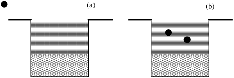
Figure 1: (a) Nucleon-nucleus scattering before the interaction begins. (b) Nucleon-nucleus first-order scattering. The black circles represent nucleons. The well represents the potential well of the nucleus. The ground state levels of the nuclear well are represented by a cross-hatch and the excited states are represented by horizontal lines. The interaction takes place in the excited state continuum with only one target nucleon from the nucleus interacting with the projectile.

The first-order approximation to Eq. (3) which is valid at suitably high energies is to assume that the projectile only interacts with one target nucleon in the nucleus Francis and Watson (1953). Applying this assumption we have

$$U=\sum_{i=1}^{A}U_{i}\approx\sum_{i=1}^{A}\hat{\tau_{0i}},$$ (4)

where $\hat{\tau_{0i}}$ is defined from Eq. (3) as

$$\hat{\tau_{0i}}=V_{0i}+V_{0i}{\cal G}_{0}{\cal Q}\hat{\tau_{0i}},$$ (5)

where the index ‘i’ represents a specific nucleon in the target. The product function ${\cal G}_{0}{\cal Q}$ is a many-body operator product, which may include effects from of the binding energy, nuclear medium, intermediate state Pauli blocking, and excited states of the nucleus. To make the problem tractable these operators are reduced to a two-body operator $({\cal G}_{0}{\cal Q})_{2B}$ by various approximations such that

$$U_{i}\approx{\tau}_{0i}=V_{0i}+V_{0i}({\cal G}_{0}{\cal Q})_{2B}{\tau}_{0i}$$ (6)

can be calculated Ray et al. (1992); Amos et al. (2000a).

In Fig. 1 we depict an interaction between the projectile and single target nucleon. Before the interaction begins the nucleus is in its ground state but as the collision proceeds the projectile enters the nuclear excited states and interacts with one bound nucleon. The $A-1$ non-active nucleons are labeled the spectator core because they play no direct role in the two-body interaction Tandy et al. (1977); Friedman (1967).

To calculate the elastic nucleon-nucleus optical potential a summation of Eq. (6) over all target nucleons is required followed by a projection onto the elastic channel

$${\cal P}U{\cal P}=\langle\Phi_{A}|\;\langle{\bf{k^{\prime}_{0},k^{\prime}_{i}}}|\;\sum_{i=1}^{A}{\tau}_{0i}\;|{\bf{k_{0},k_{i}}}\rangle\;|\Phi_{A}\rangle,$$ (7)

where $|\bf{k_{0}}\rangle$ is the momentum of the projectile nucleon with label ‘0’ and $|\Phi_{A}\rangle$ is the ground state basis of the target nucleus. For simplicity the spin and isospin characteristics of the nucleons have not been explicitly included in Eq. (7), but they will be discussed later.

The wave function of the target nucleus is usually in a convenient single particle basis used to define the nuclear structure density, $\rho_{A}$, as

$$\rho_{A}({\bf{\tilde{k}^{\prime}_{i}}},{\bf\tilde{k}_{i}})\equiv\langle\Phi_{A}^{\prime}|{\bf{\tilde{k}^{\prime}_{i}}}\rangle\;\langle{\bf\tilde{k}_{i}}|\Phi_{A}\rangle,$$ (8)

where ${\bf\tilde{k}_{i}}$ measures the momentum of target nucleon ‘i’ from the center of the struck nucleus. The definition of the optical potential is thus reduced to the traditional $t\rho$ form developed by Watson Francis and Watson (1953) and Kerman, McManus, and Thaler Kerman et al. (1959)

$${\cal P}U{\cal P}\equiv\sum_{i=1}^{A}\;\int d{\bf{\tilde{k}^{\prime}_{i}}}\;d{\bf{\tilde{k}_{i}}}\;\langle{\bf{k^{\prime}_{0},k^{\prime}_{i}}}|{\tau}_{0i}|{\bf{k_{0},k_{i}}}\rangle\rho_{A}({\bf{\tilde{k}^{\prime}_{i}}},{\bf\tilde{k}_{i}})$$ (9)

$$\delta(\bf{k^{\prime}_{0}}+{\bf{{k}^{\prime}_{i}}}-\bf{k_{0}}-{\bf{{k}_{i}}}),$$

where the delta function conserves momentum for the projectile-target nucleon system. The elastic nucleon-nucleus first-order optical potential can therefore be calculated using a nuclear density structure calculation and a two-body interaction, $\tau_{0i}$, which contains the bare nucleon-nucleon potential $V_{0i}$ as defined by Eq. (5). These two inputs are the foundation of every microscopic nucleon-nucleus optical potential calculation.

In this work we will examine the antisymmetric character of this two-body interaction including the spin and isospin dependencies in the context of the traditional Watson approximation. When discussing the two-body interaction a relationship between the two-nucleon state and the scattering state basis may be defined as

$$|\Psi_{2B}\rangle=|{\bf q},{\bf K}\rangle|S,m_{s}\rangle|T,m_{t}\rangle=\sum_{{m_{s}}_{0},{m_{t}}_{0}}\biggl{|}{\bf k_{0}},{m_{s}}_{0},{m_{t}}_{0},\;{\bf k_{i}},{m_{s}}_{i},{m_{t}}_{i}\biggr{\rangle}\biggl{\langle}{m_{s}}_{0},{m_{t}}_{0},\;{m_{s}}_{i},{m_{t}}_{i}\biggm{|}S,m_{s},T,m_{t}\biggr{\rangle}$$ (10)

where $m_{s}={m_{s}}_{0}+{m_{s}}_{i},m_{t}={m_{t}}_{0}+{m_{t}}_{i}$, ${\bf K}={{\bf k_{i}}+{\bf k_{0}}}$, ${\bf q}={\bf k_{i}}-{\bf k_{0}}$, and the identity of the particle is represented by the subscript ‘0’ or ‘$i$’. This defines the traditional two nucleon state which has by definition of the individual nucleons ${m_{s}}_{i}=\pm\frac{1}{2}$ (spin up or down) and ${m_{t}}_{i}=\pm\frac{1}{2}$ (proton or neutron). This is a basis which the $\tau_{0i}$ operator of Eq. (7) and Eq. (9) is typically calculated in.

According to the Pauli exclusion principle, since the nucleons are fermions, the scattering state $|{\bf q},{\bf K}\rangle|S,m_{s}\rangle|T,m_{t}\rangle_{2B}$, described by Eq. (10), must be antisymmetric. The possible choices are:

$$|{\bf 1}\rangle\equiv|{\bf q},{\bf K}\rangle_{sym}|S=0,m_{s}\rangle|T=1,m_{t}\rangle$$

$$|{\bf 2}\rangle\equiv|{\bf q},{\bf K}\rangle_{asym}|S=1,m_{s}\rangle|T=1,m_{t}\rangle$$

$$|{\bf 3}\rangle\equiv|{\bf q},{\bf K}\rangle_{sym}|S=1,m_{s}\rangle|T=0,m_{t}\rangle$$

$$|{\bf 4}\rangle\equiv|{\bf q},{\bf K}\rangle_{asym}|S=0,m_{s}\rangle|T=0,m_{t}\rangle.$$ (11)

These states are traditionally described in either a partial wave or helicity basis. Explicitly, for neutron-proton scattering, all four states are included. In proton-proton scattering only $T=1$ is possible so states $|{\bf 3}\rangle$ and $|{\bf 4}\rangle$ are excluded, however because of the exact identical nature of the two protons, the identity of the original nucleons is lost during the scattering process so the contributed strengths of states $|{\bf 1}\rangle$ and $|{\bf 2}\rangle$ are doubled. This is the traditional kinematical doubling for identical particles in quantum mechanics. For example in the two-body center of mass frame a scattering of 10^o is equivalent to a scattering of 170^o because the two protons cannot be differentiated thereby doubling the strength at both angles.

These results are well known but reiterated here because later we will change the character of this two-body basis to suit the many-body problem. For future reference we define equivalent to Eq. (10) and Eq. (11)

$$|\Psi_{2B}\rangle_{asym} \equiv|{\bf q},{\bf K}\rangle|S,m_{s}\rangle|T,m_{t}\rangle_{asym}$$

and in practice

$$|\Psi_{2B-np}\rangle \equiv\frac{|{\bf 1}\rangle+|{\bf 2}\rangle+|{\bf 3}\rangle+|{\bf 4}\rangle}{2}$$

$$|\Psi_{2B-pp}\rangle \equiv\frac{\sqrt{2}|{\bf 1}\rangle+\sqrt{2}|{\bf 2}\rangle}{2},$$ (12)

using the states as defined in Eq. (11). The $2B-np$ describes the traditional neutron-proton antisymmetric basis state while $2B-pp$ describes either the proton-proton or neutron-neutron basis states. To calculate a proton-¹⁶O optical potential for example we would sum up eight $\tau_{0i}$ interactions in the traditional proton-proton basis and eight $\tau_{0i}$ interactions in the traditional neutron-proton basis because the proton projectile interacts with either one of eight protons or eight neutrons in the target nucleus. They are also weighted with the appropriate single particle ¹⁶O density contribution

$${\cal P}U{\cal P}\equiv$$

$$8 \int d{\bf{\tilde{k}^{\prime}_{i}}}\;d{\bf{\tilde{k}_{i}}}\;\langle\Psi_{2B-pp}|{\tau}_{0i}|\Psi_{2B-pp}\rangle\rho_{proton}({\bf{\tilde{k}^{\prime}_{i}}},{\bf\tilde{k}_{i}})$$

$$+ 8 \int d{\bf{\tilde{k}^{\prime}_{i}}}\;d{\bf{\tilde{k}_{i}}}\;\langle\Psi_{2B-np}|{\tau}_{0i}|\Psi_{2B-np}\rangle\rho_{neutron}({\bf{\tilde{k}^{\prime}_{i}}},{\bf\tilde{k}_{i}}),$$

akin to Eq. (9). The validity of this calculation in the context of the many-body problem will be examined in section IV.

III Practical first-order many-body calculations

The two-body interaction calculated in many microscopic nucleon-nucleus interactions is Eq. (5)

$$\hat{\tau_{0i}}=V_{0i}+V_{0i}{\cal G}_{0}{\cal Q}\hat{\tau_{0i}}.$$

As stated previously, ${\cal G}_{0}{\cal Q}$ is a product of many-body operators which involve the propagation of two nucleons through a nucleus which is not in the ground state. The spectator core directly affects the two nucleons’ propagation, identity, and interaction. In this section we will discuss the two most common methods which make this operator suitable for calculation. For a more exhaustive summary of these two techniques see Ref. Amos et al. (2000a).

III.1 Folding $t$ operator approach

The first-order optical potential involves a sum of two-body interactions between the projectile and the target nucleons

$$U=\sum_{i=1}^{A}\hat{\tau_{0i}},$$ (14)

where the operator $\hat{\tau_{0i}}$ is

$$\hat{\tau_{0i}} = V_{0i}+V_{0i}{\cal G}_{0}{\cal Q}\hat{\tau_{0i}}$$ (15)

$$= V_{0i}+V_{0i}{\cal G}_{0}\hat{\tau_{0i}}-V_{0i}{\cal G}_{0}{\cal P}\hat{\tau_{0i}}$$

$$= {\cal T}_{0i}-{\cal T}_{0i}{\cal G}_{0}{\cal P}\hat{\tau_{0i}},$$

which is derived by using the relationship ${\cal P}+{\cal Q}\equiv 1$. This procedure successfully removes operator ${\cal Q}$ from the calculation with the cost of a new operator ${\cal T}_{0i}$.

For elastic scattering only ${\cal P}\hat{\tau_{0i}}{\cal P}$ need to be considered. Explicitly it appears as

$$\hat{\tau_{0i}}={\cal T}_{0i}-{\cal T}_{0i}\frac{1}{(E-E_{A})-h_{0}+i\varepsilon}\hat{\tau_{0i}},$$ (16)

where ${\cal T}_{0i}$ is defined as the solution of the sum of nucleon-nucleon interactions as the two nucleons propagate through the many-body medium

$${\cal T}_{0i}=V_{0i}+V_{0i}{\cal G}_{0}{\cal T}_{0i}.$$ (17)

Since Eq. (16) is a simple two-body integral equation, the principal problem is to find a solution of Eq. (17), which still has a many-body character due to the propagator

$${\cal G}_{0}=(E-h_{0}-H_{A}+i\varepsilon)^{-1},$$ (18)

where $H_{A}$ is the many-body Hamiltonian of the target nucleus. If the propagator ${\cal G}_{0}$ is expanded within a single particle description, one obtains to first-order Chinn et al. (1995a, 1993); Elster et al. (1997)

$$G_{i}=[(E-E^{i})-h_{0}-h_{i}-W_{i}+i\varepsilon]^{-1},$$ (19)

where $h_{i}$ is the kinetic energy of the $i$th target particle and $W_{i}=\sum_{j\neq i}v_{ij}$. The quantity $W_{i}$ represents the mean field acting between the struck target nucleon and the residual (A-1) nucleus made from summing up all the individual nucleon-nucleon potentials contained within the spectator core. The operator ${\cal T}_{0i}$ of Eq.(17) is then approximated as

$${\cal T}_{0i} \approx =V_{0i}+V_{0i}G_{i}\tau_{0i}$$ (20)

$$= {\cal T}_{2B}+{\cal T}_{2B}G_{0}W_{i}G_{i}{\cal\tau}_{0i},$$

where the pure nucleon-nucleon interaction operator ${\cal T}_{2B}$ is defined as

$${\cal T}_{2B}=V_{0i}+V_{0i}G_{0}{\cal T}_{2B},$$ (21)

and

$$G_{0}=[(E-E^{i})-h_{0}-h_{i}+i\varepsilon]^{-1},$$ (22)

is the free two-body propagator. Finally, the two-body equation for the medium modified two-body operator that appears in Eq. (16) may be defined as

$${\cal T}_{0i} \approx {\cal T}_{2B}+{\cal T}_{2B}G_{0}W_{i}G_{i}{\cal T}_{0i}$$

$${\cal T}_{0i} \approx {\cal T}_{2B}+{\cal T}_{2B}G_{0}{T}_{iC}G_{0}{\cal T}_{0i},$$ (23)

where

$${T}_{iC}=W_{i}+W_{i}+G_{0}{T}_{iC},$$ (24)

is the sum of all interactions between the excited nucleon and the spectator core.

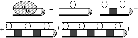
Figure 2: A graphical depiction of Eq. (26) which represents the t-operator method for calculating the medium effects for nucleon-nucleus scattering. The nucleon-nucleon interaction is represented by the ellipses (${\cal T}_{2B}$). The mean-field of the core nucleus, ($T_{iC}$), is represented by the black squares. The spectator core is represented by the thick black line at the bottom which exists throughout the entire calculation. The two top thin black lines represent the two active nucleons which exist in the continuum of the nuclear well (as depicted in Fig. 1). Only at the beginning of the calculation does the ground state of the nucleus exist as denoted by the semi-circle imprinted by an ‘A’. There is never an explicit interaction between the top-line projectile and the spectator core in this theory.

The projectile nucleon interacts with the a struck target nucleon through ${\cal T}_{2B}$ and the nuclear core interacts with this same stuck nucleon by ${T}_{iC}$. Therefore Equation (23) can be written as a set of two coupled equations

$${\cal T}_{0i} = {\cal T}_{2B}+{\cal T}_{2B}G_{0}\hat{X_{i}}$$

$$\hat{X_{i}} = T_{iC}G_{0}{\cal T}_{0i},$$ (25)

where the homogeneous equation represents the bound state and the driving term in the first equation represents the projectile interacting with the bound state. Iterating Eq. (23) we may understand the physical mechanism better

$${\cal T}_{0i}|\Phi_{A}\rangle = {\cal T}_{2B}|\Phi_{A}\rangle$$ (26)

$$+ {\cal T}_{2B}G_{0}{T}_{iC}G_{0}{\cal T}_{2B}|\Phi_{A}\rangle$$

$$+ {\cal T}_{2B}G_{0}{T}_{iC}G_{0}{\cal T}_{2B}G_{0}{T}_{iC}G_{0}{\cal T}_{2B}|\Phi_{A}\rangle$$

$$+ \ldots,$$

which is graphically represented in Fig. 2. Equations(25-26) is an approximation to Faddeev’s exact theory for three bodies Faddeev (1965) which contains three coupled equations. It is approximate because the projectile never interacts with the spectator core while in a true Faddeev three-body theory all three particles interact on equal footing with each other, this distinction will be utilized later. A good summary of this approximate three-body theory (projectile, target nucleon, and spectator core) can be found in Refs. Tandy et al. (1977); Chinn et al. (1995a, 1993).

III.2 Folding $g$ operator approach

There is another popular approach to reducing the operator ${\cal G}_{0}{\cal Q}$ from a many-body operator to a two-body operator. The two-body interaction, as stated previously, used in most nucleon-nucleus interactions involves calculating Eq. (5)

$$\hat{\tau_{0i}}=V_{0i}+V_{0i}{\cal G}_{0}Q\hat{\tau_{0i}}.$$

In the traditional g-operator method (see for example Refs. Amos et al. (2000a); Arellano et al. (1990, 1995, 1996)) this equation is simplified to

$$\hat{\tau_{0i}}\approx g_{0i}=V_{0i}+V_{0i}{\cal G_{Q}}g_{0i},$$ (27)

where the propagator, ${\cal G}_{0}$ is modified to represent the medium of the nuclear bound state signified with the subscript ${\cal Q}$. The $V_{0i}$ is still the bare nucleon-nucleon potential. As with the t-operator approach it is usually assumed that there is only one active target nucleon and the rest provide a mean field Amos et al. (2000a). The medium effects contained within the propagator can be developed using various schemes. One method is to treat the nucleus like an infinite Fermi gas and derive spectral functions. Another is to include intermediate Pauli-blocking directly by using an operator which only allows entering a state which is above the Fermi level. This provides a similar mechanism to the folding $t$ approach which includes only excited states in the calculation via the projector ${\cal Q}$. The iterative form of the $g$ equation is

$$g_{0i}=V_{0i}+V_{0i}{\cal G_{Q}}V_{0i}+V_{0i}{\cal G_{Q}}V_{0i}{\cal G_{Q}}V_{0i}+\ldots,$$ (28)

which is similar in structure to Eq. (26) of the t-operator approach in which the total reaction can be broken into interactions with either the two nucleons ($V_{0i}$) or the spectator core and the target nucleon ($\cal G_{Q}$) to first order. This theory has a rich history which was begun by Brueckner Brueckner and Levinson (1955); Bethe et al. (1963) and is still active Amos et al. (2000a).

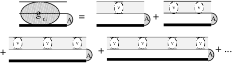
Figure 3: A graphical depiction of Eq. (28) which represents the g-operator method of calculating the medium effects for nucleon-nucleus scattering. The nucleon-nucleon interaction is represented by the ellipses ($V$). The propagator has been modified to represent the mean-field effects of the core nucleus (the grayed background). The spectator core is represented by the bottom thick black line which exists throughout the entire calculation. The two top thin black lines represent the two active nucleons which exist in the continuum of the nuclear well (as depicted in Fig. 1). Only at the beginning (and also end for elastic scattering) of the calculation does the ground state of the nucleus exist as denoted by the semi-circle imprinted by an ‘A’. There is never an explicit interaction between the top-line projectile and the spectator core in this theory.

In Fig. 3 a graphical depiction of the g-operator theory is shown where the free propagator has been ‘grayed’ in to show that it has been modified. In g-operator theory the potential, $V_{0i}$, is the active operator in contrast with t-operator theory which uses ${\cal T}_{2B}$ as its focus. Both the $g$ operator method and the $t$ operator method allow the modification of the two nucleon interaction via changes in the propagator. These changes represent the effects of the nuclear medium that the struck nucleon is bound to and the projectile is moving through. These ‘medium effects’ have been shown to be important in a variety of different calculations Amos et al. (2000a); Chinn et al. (1995a, b), notably below 200 MeV laboratory energy for the incoming nucleon. In both formulations the interaction between the projectile and the spectator core is usually ignored. Again this approximation will be exploited in the next section.

IV Antisymmetrization

Watson and collaborators Francis and Watson (1953); Takeda and Watson (1955) concluded that the use of the antisymmetrized two nucleon interaction was all that was required in high energy calculations for a correct Pauli principle inclusion. The argument was qualitative in nature but powerful. A chance of significant overlap of the projectile wave function with more than one target nucleon is small for scattering events with projectiles of high energy. If overlap is inconsequential, the calculation may be reduced to a two-body problem and thus only two-body antisymmetrization is required Takeda and Watson (1955). This will be referred to as the ‘Watson approximation’ in the remainder of this work.

Figure 4: An outline of the spectator expansion. The top drawing represents the first-order calculation with only two active particles, the projectile and one target nucleon. The second order calculation involves two target nucleons, etc.

Many modern microscopic scattering theories are organized using a spectator expansion as depicted in Fig. 4. The first-order calculation only scatters from nucleon $i$. The second-order calculation involves double-scattering events from nucleons $i$ and $j$. The Watson approximation, based on wave function overlap, is consistent with the spectator expansion which only antisymmeterizes the active particles.

Historically however there have been examples in which a theory has been revised to include the spectators as part of the antisymmetrization process. For example in nuclear physics the representation of the ground state of a nucleus improves when the wave function is completely antisymmetrized. Most models only include interactions of nearest neighbors, however all nucleons in the nucleus interact indirectly via the Pauli principle and thus the importance of an antisymmetrization scheme for the whole nucleus.

An older example is that of spin. Although spin is added to the non-relativistic Schrödinger wave functions, the most significant role it plays in atomic physics is to produce the correct fermionic combinatorics by assigning each electron a unique orbital. The actual interactions which include spin are relatively weak and are often ignored. It is with these precedents plausible to develop a theory which includes both active and spectator nucleons in its antisymmetrization scheme in contrast to the Watson approximation. This is the goal of the next subsections where we will examine the role and identity of the projectile in a many-body optical potential scattering theory.

IV.1 A distinguishable projectile

In traditional nucleon-nucleon scattering theory the label of projectile is often given to one of the nucleons in the initial state. This label is not an intrinsic quality and therefore not an adequate quantum number. During the scattering process the role of the projectile is not unique, its identity is lost, and only by convention do we choose the final state projectile to have the same isospin projection as the initial projectile.

In exact Faddeev elastic nucleon-deuteron scattering the projectile is also not an intrinsic label Glöckle et al. (1996). The projectile is defined, by convention, in both the initial and final states as the nucleon which is not bound. During the intermediate states of the scattering process this characteristic is lost and all nucleons are on equal identity footing in the Faddeev scheme.

In nucleon-nucleus scattering is the projectile also indistinguishable? A condition for the projectile in nucleon-nucleus scattering is that it is ‘fast’. This argument was given by Watson and collaborators in Refs. Francis and Watson (1953); Watson (1953) and has some merit. On average, in the center of mass frame of the nucleon-nucleus system, the free projectile nucleon has a momentum magnitude a factor of $A$ times greater than the target nucleon. This constraint is however not sufficiently strong to warrant quantum distinguishability because it is only a mean kinematical expectation.

The strongest criteria for distinguishability of the projectile comes from the approximate form of the theory itself. To create the optical potential one sums up over all the target nucleons (see Eq. (7)). This summation could imply that the target nucleon that is struck in the optical potential theory is actually the average composite nucleon of the nucleus. For example in an $N=Z$ nucleus the average target nucleon is half proton and half neutron. The theory, because of its approximate nature, has created an artificial distinguishable composite nucleon target separable from the projectile during the entire collision process. Since this composite half-proton and half-neutron target nucleon has no possibility to be considered identical with the projectile then all traditional kinematic exchange factors which double the strength of the transition operator for either proton-proton or neutron-neutron scattering should be ignored as the composite nucleus optical potential is built via Eq. (7). The implication of this is simply that all traditional neutron-neutron or proton-proton two-body amplitudes are cut in half when used in summing the complete many-body optical potential

$$|\Psi_{CM-np}\rangle \equiv|\Psi_{2B-np}\rangle$$

$$|\Psi_{CM-pp}\rangle \equiv\frac{|\Psi_{2B-pp}\rangle}{\sqrt{2}},$$ (29)

using the notation established in Eq. (12). This effective theory is a manifestation of the approximate averaging made in the optical potential theory. As an example of a calculation using this modification we show the proton-¹⁶O optical potential given in traditional form by Eq. (LABEL:eq4.14b) is now modified to be

$${\cal P}U_{CM}{\cal P}\equiv$$

$$8 \int d{\bf{\tilde{k}^{\prime}_{i}}}\;d{\bf{\tilde{k}_{i}}}\;\langle\frac{\Psi_{2B-pp}}{\sqrt{2}}|{\tau}_{0i}|\frac{\Psi_{2B-pp}}{\sqrt{2}}\rangle\rho_{proton}({\bf{\tilde{k}^{\prime}_{i}}},{\bf\tilde{k}_{i}})$$

$$+ 8 \int d{\bf{\tilde{k}^{\prime}_{i}}}\;d{\bf{\tilde{k}_{i}}}\;\langle\Psi_{2B-np}|{\tau}_{0i}|\Psi_{2B-np}\rangle\rho_{neutron}({\bf{\tilde{k}^{\prime}_{i}}},{\bf\tilde{k}_{i}}).$$

In section V we will show results of this type of calculation under the ‘CM’ label (composite model).

This ‘composite model’ theory does have disadvantages. The theory should be able to be extended to such processes as charge exchange reactions but it no longer has the apparatus for their inclusion since each target nucleon now only contains a fraction of charge. In the next subsection we will look at a different, more appealing, theoretical model for antisymmetrization.

IV.2 Projectile as quantum label

In the first-order many-body theory there is a difference between the projectile nucleon and the struck target nucleon which has not yet been exploited. In Fig. 2, the $t$-folding operator model shows that the struck target nucleon is acted upon by the mean field and thus explicitly interacts with the nucleus while the projectile does not. This differentiates the two nucleons and is true throughout the whole calculation. The projectile nucleon at all times carries the characteristic that it is absent an interaction with the spectator core. Conversely, the struck target nucleon interacts via a mean field with the spectator core throughout the entire reaction. If the $g$-folding theory has the projectile interact with the infinite nuclear matter of the core than it contains higher order terms Amos et al. (2000b) and the projectile will be difficult to distinguish. However if the theory does not have the projectile interact with the nuclear matter core, as in Fig. 3, than this same differential characteristic may be exploited.

Introducing a new quantum number formalism for the many-body interaction basis, where $|a,m_{a}\rangle$ is the addition, Eq. (10) now becomes

$$|\Psi_{MB}\rangle\equiv|\Psi_{2B}\rangle|a,m_{a}\rangle,$$ (31)

where the $MB$ still represents a two-body interaction but taken within the many-body context of nucleon-nucleus scattering. The additional quantum number $a$ is a vector fundamentally belonging to the SU(2) group for one nucleon (as do spin and isospin) which denotes a new intrinsic quality created by the approximate form inherent in the optical potential theory: $m_{a}=+\frac{1}{2}$ if an interaction is not required with the spectator core and $m_{a}=-\frac{1}{2}$ if it is required. In all pure first-order optical potential elastic scattering theories the projectile has $m_{a}=+\frac{1}{2}$ because there is no explicit interaction with the spectator, all other target nucleons have $m_{a}=-\frac{1}{2}$ because they interact via the mean field and single particle density.

$a$	state	$m_{a}$	pictorial	Coef.	example theory
		1	$\uparrow\uparrow$	1	nucleon-nucleon
1	symmetric	0	$\uparrow\downarrow+\downarrow\uparrow$	.5	optical potential
		-1	$\downarrow\downarrow$	1	exact Faddeev
0	antisymmetric	0	$\uparrow\downarrow-\downarrow\uparrow$	.5	optical potential

Table 1: A description of the combination of quantum number $a$ from the projectile and the struck nucleon. This quantum number represents an intrinsic quantity of each nucleon involved in a many-body scattering theory and belongs to the SU(2) group (as does spin and isospin). Coef. is the Clebsch-Gordan coefficient squared and represents the probability. The Faddeev Faddeev (1961) and two-body nucleon-nucleon scattering theories are always symmetric while the optical potential is mixed in symmetry for the $a$ quantum number because of its approximate nature.

The $a$ quantum number adds like the spin and isospin quantum numbers, ${\bf a=a_{0}+a_{i}}$ and $m_{a}={m_{a}}_{0}+{m_{a}}_{i}$. An analogy to isospin can be clearly elucidated. The most significant difference between isospin flavors (neutron or proton) is the effect of the coulomb interaction, likewise the difference between $a$ flavors (projectile and non-projectile) is the effect of the spectator core nucleon’s interaction. In Table 1 we summarize the combinatorics of this new vector. Importantly this new many-body basis does not change the nature of the fundamental nucleon-nucleon interaction, it is only a placeholder vector symbolizing the status of the interaction with the spectator core. The reason for its existence is solely because the Faddeev theory is approximated in developing the optical potential, the additional quantum numbers are the relics of that approximation. The Hamiltonian for the nucleon-nucleon interaction conserves this new quantum number and the measurement of it commutes with all dynamical variables. The significance of this quantum number is the distinguishability it produces is needed in the many-body context. This becomes clearer if we re-examine the t-operator method of Eq. (26):

$${\cal T}_{0i}|\Phi_{A}\rangle = {\cal T}_{2B}|\Phi_{A}\rangle$$

$$+ {\cal T}_{2B}G_{0}{T}_{iC}G_{0}{\cal T}_{2B}|\Phi_{A}\rangle$$

$$+ {\cal T}_{2B}G_{0}{T}_{iC}G_{0}{\cal T}_{2B}G_{0}{T}_{iC}G_{0}{\cal T}_{2B}|\Phi_{A}\rangle$$

$$+ \ldots$$

The operator ${\cal T}_{2B}$ represents the fundamental nucleon-nucleon interaction and although a quantum number has been added this interaction remains unchanged

$$\sum_{T}\langle a=1,m_{a}=0|\langle\Psi_{2B}|{\cal T}_{2B}|\Psi_{2B}\rangle|a=1,m_{a}=0\rangle$$ (32)

$$\equiv \sum_{T}\langle a=0,m_{a}=0|\langle\Psi_{2B}|{\cal T}_{2B}|\Psi_{2B}\rangle|a=0,m_{a}=0\rangle$$

$$\equiv .5\;\sum_{T}\langle\Psi_{2B}|{\cal T}_{2B}|\Psi_{2B}\rangle,$$

assuming that the nucleon-nucleon potential is isospin ($T$) independent. The factor of .5 recognizes that the new quantum number, $a$, divides the original space in two, a symmetric ($a=1$) and antisymmetric ($a=0$) part.

In every final channel of the ${\cal T}_{2B}$ operator the struck target nucleon must be differentiated from the projectile to calculate the ${T}_{iC}$ operator, which is the interaction between the target nucleon and the spectator core

$$\biggl{\langle}a_{i}=\frac{1}{2},{m_{a}}_{i}=+\frac{1}{2}\biggm{|}T_{iC}\biggm{|}a_{i}=\frac{1}{2},{m_{a}}_{i}=+\frac{1}{2}\biggr{\rangle}=0$$

$$\biggl{\langle}a_{i}=\frac{1}{2},{m_{a}}_{i}=-\frac{1}{2}\biggm{|}T_{iC}\biggm{|}a_{i}=\frac{1}{2},{m_{a}}_{i}=-\frac{1}{2}\biggr{\rangle}\neq 0,$$

where the first equation represents the interaction, with null result, of the projectile with the core $A-1$ nucleons while the second equation represents the target nucleon interacting with the core. Likewise in the initial and final elastic channels of the complete reaction the struck nucleon is bound using the $|\Phi_{A}\rangle$ basis to describe the nucleus. In this modified version we add the $a_{i},{m_{a}}_{i}$ quantum number description to this basis in which only $m_{a}=-\frac{1}{2}$ is non zero.

This new two-body $|a,m_{a}\rangle$ eigenvector is always symmetric for nucleon-nucleon scattering $(a=1,m_{a}=-1)$ where there are no other interaction requirements and it is also always symmetric for Faddeev nucleon-deuteron scattering ($a=1,m_{a}=+1$) where all interaction requirements are explicitly included. Thus because both nucleons have the same projections in these exact theories all protons can still be considered identical. Conversely, all approximate first-order optical potential theories allow the $|a,m_{a}\rangle$ eigenvector to be mixed symmetric (50%) or antisymmetric (50%) with an $m_{a}=0$. This is an additional degree of freedom introduced specifically by the approximation in the first-order optical potential theory.

Because the optical potential theory distinguishes between projectile and target nucleons the new quantum $a$ number may be exchanged either symmetrically or antisymmetrically as long as the overall scattering amplitude remains antisymmetric. In the Watson approximation the states represented by $a=1$ are the only physical states included. The many-body theory, presented in this work, allows both $a=0$ and $a=1$ states. Its behavior in the many-body optical potential theory fundamentally changes the acceptable basis from which it operates.

Applying this new quantum number to neutron-proton scattering in the many-body context it is again noted that the addition does not change the strength of the two nucleon scattering phase space because this quantum number represents an external interaction. The new neutron-proton scattering amplitude in a many-body context now has a total of eight states:

$$|{\bf 1_{MB}}\rangle\equiv|{\bf q},{\bf K}\rangle_{sym}|S=0,m_{s}\rangle|T=1,0\rangle|a=1,0\rangle$$

$$|{\bf 2_{MB}}\rangle\equiv|{\bf q},{\bf K}\rangle_{asym}|S=1,m_{s}\rangle|T=1,0\rangle|a=1,0\rangle$$

$$|{\bf 3_{MB}}\rangle\equiv|{\bf q},{\bf K}\rangle_{sym}|S=1,m_{s}\rangle|T=0,0\rangle|a=1,0\rangle$$

$$|{\bf 4_{MB}}\rangle\equiv|{\bf q},{\bf K}\rangle_{asym}|S=0,m_{s}\rangle|T=0,0\rangle|a=1,0\rangle$$

$$|{\bf 5_{MB}}\rangle\equiv|{\bf q},{\bf K}\rangle_{sym}|S=1,m_{s}\rangle|T=1,0\rangle|a=0,0\rangle$$

$$|{\bf 6_{MB}}\rangle\equiv|{\bf q},{\bf K}\rangle_{asym}|S=0,m_{s}\rangle|T=1,0\rangle|a=0,0\rangle$$

$$|{\bf 7_{MB}}\rangle\equiv|{\bf q},{\bf K}\rangle_{sym}|S=0,m_{s}\rangle|T=0,0\rangle|a=0,0\rangle$$

$$|{\bf 8_{MB}}\rangle\equiv|{\bf q},{\bf K}\rangle_{asym}|S=1,m_{s}\rangle|T=0,0\rangle|a=0,0\rangle$$

(34)

which are antisymmetric. The first number in the isospin and antisymmetric bra-kets represent the full vector, the second number represents the projection. All eight states are individually half the strength of the four for two-body scattering listed in Eq. (11) because the new quantum number $a$ splits the traditional space into two and renormalizes them (the coefficient of .5 in Table 1). If the nucleon-nucleon potential is isospin independent (if the $T=1$ state amplitudes are the same as the $T=0$ amplitudes given an identical momentum-spin space) then the eight states reduce to only four unique states. The combined character and strength of the four states are then the same for the traditional two-body and many-body neutron-proton interactions. The scattering amplitude therefore does not change with the addition of the new quantum number in the neutron-proton case, it is only an additional placeholder. The proton and neutron have already been differentiated by isospin so this new addition is redundant and inconsequential as expected.

The many-body proton-proton scattering amplitude has a total of four states which are antisymmetric (those that have T=1 designation only)

$$|{\bf 1_{MB}}\rangle\equiv|{\bf q},{\bf K}\rangle_{sym}|S=0,m_{s}\rangle|T=1,1\rangle|a=1,0\rangle$$

$$|{\bf 2_{MB}}\rangle\equiv|{\bf q},{\bf K}\rangle_{asym}|S=1,m_{s}\rangle|T=1,1\rangle|a=1,0\rangle$$

$$|{\bf 5_{MB}}\rangle\equiv|{\bf q},{\bf K}\rangle_{sym}|S=1,m_{s}\rangle|T=1,1\rangle|a=0,0\rangle$$

$$|{\bf 6_{MB}}\rangle\equiv|{\bf q},{\bf K}\rangle_{asym}|S=0,m_{s}\rangle|T=1,1\rangle|a=0,0\rangle$$

(35)

which for comparison use the same numbering scheme as the neutron-proton states listed in Eq. (34). These states have distinct differences from their pure nucleon-nucleon counterparts. Two of the states include even momentum space-spin space product wave functions which were not allowed in the traditional two-body proton-proton case. States $|{\bf 5_{MB}}\rangle$ and $|{\bf 6_{MB}}\rangle$ include formally forbidden scattering states like ${}^{3}S_{1}$ and ${}^{1}P_{1}$ written in traditional partial wave ${}^{2S+1}L_{J}$ notation. Also there is another significant change for proton-proton scattering in the many-body context. The protons are no longer considered identical thus the traditional kinematical doubling for identical particles described earlier will no longer occur. The protons are no longer identical because of the new $a$ quantum number, thus they are now on the same footing as the neutron-proton interaction kinematically.

In summary this new quantum number, to first approximation, does not change the character of the neutron-proton interaction but the proton-proton interaction now mimics the neutron-proton interaction at half strength (only half the number of states are possible)

$$|\Psi_{MB-np}\rangle \equiv|\Psi_{2B-np}\rangle$$

$$|\Psi_{MB-pp}\rangle \equiv\frac{|\Psi_{2B-np}\rangle}{\sqrt{2}}.$$ (36)

This is a manifestation of the approximate nature of the first order optical potential and is not a characteristic of the fundamental force. As an example of a calculation using this modification we show the proton-¹⁶O optical potential given in traditional form by Eq. (LABEL:eq4.14b) is now modified to be

$${\cal P}U_{MB}{\cal P}\equiv$$

$$8 \int d{\bf{\tilde{k}^{\prime}_{i}}}\;d{\bf{\tilde{k}_{i}}}\;\langle\frac{\Psi_{2B-np}}{\sqrt{2}}|{\tau}_{0i}|\frac{\Psi_{2B-np}}{\sqrt{2}}\rangle\rho_{proton}({\bf{\tilde{k}^{\prime}_{i}}},{\bf\tilde{k}_{i}})$$

$$+ 8 \int d{\bf{\tilde{k}^{\prime}_{i}}}\;d{\bf{\tilde{k}_{i}}}\;\langle\Psi_{2B-np}|{\tau}_{0i}|\Psi_{2B-np}\rangle\rho_{neutron}({\bf{\tilde{k}^{\prime}_{i}}},{\bf\tilde{k}_{i}}).$$

The results of nucleon-nucleon scattering and exact Faddeev scattering are left unaffected by this work as expected.

Exchange of ${m_{a}}$ is not included explicitly in the many-body amplitude but it is assumed to exist. Since the $m_{a}$ quantum number is tied directly with the identity of the projectile in proton-proton (or neutron-neutron) scattering it shares many similarities with the $m_{t}$ quantum number in neutron-proton scattering. In two-body scattering the significance of isospin exchange does not affect the final result. The distinguishable calculation (not including isospin) is the exact same as the indistinguishable result (including isospin) because the projectile nucleon by convention always carried the same isospin component. The same is true with this new quantum number $a$ in the many-body case. The projectile always carries the $m_{a}=+\frac{1}{2}$ component so target exchange is irrelevant to the final result. Irrelevant does not mean that it does not happen, there is no need to add an explicit exchange mechanism for quantum label $m_{a}$ to the nucleon-nucleus theory. This feature of exchange was noted by Kowalski in Ref. Kowalski (1984).

There have been two new antisymmetrization models presented. The first, the composite model (CM), treats the target as distinguishable and therefore not identical. The second model adds a new quantum number $a$ to treat two protons as indistinguishable but no longer identical. The latter model is more sophisticated, involves exchange in a natural way, and treats antisymmetrization with a many-body formalism (MB). All three models have the same neutron-proton amplitudes but are differentiated by how they treat the proton-proton (and neutron-neutron) amplitudes. In the next section we will show comparisons between the traditional Watson approximation, the composite model, and the many-body model.

V Results

Comparisons will be made between experimental data and calculations which involve a folding, energy fixed, $t$ operator approach (described in section III.1 and further in Ref. Elster et al. (1997)). The medium effects ($T_{iC}$) have been set to zero so that only the Born term is calculated in Fig. 2. The reasoning for not including any medium modifications is so that the differences between the strengths of the antisymmetric techniques can be clearly elucidated. Medium affects are only significant with projectile energies below 200 MeV Chinn et al. (1993) so most comparisons in this section are made with energies of at least 200 MeV. To further ascertain the significance of the antisymmetric technique the same Dirac-Hartree nuclear structure calculation Horowitz et al. (1991) and the same nucleon-nucleon potential Stoks et al. (1994), fit to the 1993 dataset of nucleon-nucleon observables, is used in all calculations unless otherwise noted. Beyond these two inputs there are no adjustable parameters.

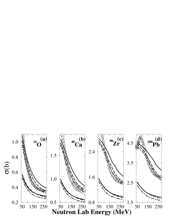
Figure 5: Four total and inelastic (reaction) neutron-nucleus cross section from four different nuclear targets. The upper lines are calculations of the total cross section while the lower lines represent the inelastic cross section. The solid line is the two-body Watson approximation,2B, the dashed line is the many-body calculation, MB, and the dashed-dotted line represents the composite model (CM). All calculations use a Dirac-Hartree density Horowitz et al. (1991) and the Nijmegen nucleon-nucleon potential Stoks et al. (1994) and a full-folding procedure Elster et al. (1997). The neutron total cross section data (diamonds) are taken from Ref. Finlay et al. (1993). There is systematic error which is roughly represented by the size of the diamonds Abfalterer et al. (2001).

The Watson approximation will be referred to as ‘2B’ (discussed first in section I), the ‘CM’ will be the composite model (discussed in section IV.1), and the many-body antisymmetry will be ‘MB’(discussed in section IV.2). To summarize the differences between the three theoretical models, the 2B model uses the same two-body interaction used in nucleon-nucleon and nucleon-deuteron scattering, the CM model cuts all proton-proton and neutron-neutron amplitudes in half, and the MB model replaces the proton-proton and neutron-neutron amplitudes with the neutron-proton amplitudes and also cuts them in half. The end result is that the strength of the $m_{t}=\pm 1$ amplitudes developed in this work are roughly half that of the the traditional Watson two-body amplitudes. It will be shown that this dramatic reduction leads to an improvement in the theoretical fit to experimental data. Then an examination of why the Watson approximation has been successful for five decades and why now the need for modification.

In Fig. 5 we compare these three calculations (2B,MB,CM) on neutron-nucleus total and inelastic cross sections for four doubly magic targets, ¹⁶O,⁴⁰Ca,⁹⁰Zr, and ²⁰⁸Pb. The over prediction of the Watson approximation (solid line) in the range of validity for this calculation ($\geq$ 200 MeV) stands out while the other calculations (MB:dashed, CM:dashed-dotted) do much better. This over prediction for the total cross section using the traditional Watson approximation signifies that the strength of the effective interaction designated by the optical potential is much too large. The data and calculation have a high level of precision such that this difference is indeed real and significant (sometimes as high as 20%). The many-body and composite model do much better by reducing the strength of the neutron-neutron amplitudes which are inherent in the nucleon-nucleus optical potential calculation.

The inelastic cross section calculations are included for future reference. An interesting facet worthy of study is that surprisingly the two-body calculation roughly matches the many-body result (but not the composite result). Therefore the many-body result mainly reduces only the elastic cross section while the composite model reduces amplitudes which contribute to both the elastic and inelastic cross section.

Figure 6: Extreme forward differential cross section calculations and experimental data for a proton on ¹⁶O, a proton on ⁴⁰Ca, and a proton on ²⁰⁸Pb at 200 MeV proton laboratory energy. The calculation procedure and inputs are the same as Fig. 5. The solid line represents the Watson approximation (2B) while the dashed line represents the many-body antisymmetrization (MB) and the dashed-dotted line represents the composite model (CM). The data points are represented by circles and are taken from Refs. Stephenson (1985); Hutcheon et al. (1988); Gi (1987).

Proton-nucleus differential cross section calculations at the extreme forward angles for ¹⁶O,⁴⁰Ca, and ²⁰⁸Pb at a proton lab energy of 200 MeV are shown in Fig. 6. Again the 2B Watson calculation (solid line) over-predicts the data points at the extreme forward angles while the other calculations (MB:dashed, CM:dashed-dotted) compare better with experiment. Although these differences may appear slight they are actually rather significant because this is a logarithmic graph. Once again the use of the Watson approximation (2B) leads to an effective nucleon-nucleon potential which has too large a strength (as much as 50%!). Both the many-body antisymmetrization (MB) and the composite model (CM) come closer to the experimental values in all cases tested at and above this energy. Because these are proton projectiles a coulomb force has been added Chinn et al. (1991). The systematic use of first neutrons (in Fig. 5) and then protons (in Fig. 6) as projectiles, resulting in the same over prediction for the Watson approximation calculation, removes the coulomb interaction as a source of the discrepancy.

The importance of fitting accurately the forward angles for proton-nucleus elastic differential cross sections must be emphasized. It is the most significant part of the cross section and therefore of importance to understand if the strength is to be calculated accurately using an effective interaction. Too often these discrepancies are missed because of the range and logarithmic nature of the experimental measurements. For example these differences are barely noticeable when the same data and calculations are graphed over a larger range as in Figs. 7-9.

Figure 7: The differential cross section ($d\sigma/d\Omega$), analyzing power or polarization ($A_{y}$), and the spin transfer ($Q$) for a proton interacting with ¹⁶O at a laboratory energy of 200 MeV. The data are the circles and were taken from Ref. Stephenson (1985). The solid line represents the Watson approximation (2B) while the dashed line is the many-body antisymmetrization model (MB). For graphical clarity the composite model (CM), which closely mimics MB, is not included. The calculation methods and inputs are described in Fig. 5 and the text.

Figure 8: The differential cross section ($d\sigma/d\Omega$), analyzing power or polarization ($A_{y}$), and the spin transfer ($Q$) for a proton interacting with ⁴⁰Ca at a laboratory energy of 200 MeV. The data are the circles and were taken from Ref. Stephenson (1985). The solid line represents the Watson approximation (2B) while the dashed line is the many-body antisymmetrization model (MB). For graphical clarity the composite model (CM), which closely mimics MB, is not included. The calculation methods and inputs are described in Fig. 5 and the text.

Figure 9: The differential cross section ($d\sigma/d\Omega$), analyzing power or polarization ($A_{y}$), and the spin transfer ($Q$) for a proton interacting with ²⁰⁸Pb at a laboratory energy of 200 MeV. The data are the circles and were taken from Ref. Stephenson (1985). The solid line represents the Watson approximation (2B) while the dashed line is the many-body antisymmetrization model (MB). For graphical clarity the composite model (CM), which closely mimics MB, is not included. The calculation methods and inputs are described in Fig. 5 and the text.

The complete elastic experimental observables for a proton scattering off of ¹⁶O,⁴⁰Ca, and ²⁰⁸Pb respectively are shown in Figs. 7-9. The top graph in each figure is the same differential cross section that was depicted in Fig. 6 except now a larger angle range is used. The middle graph is the spin polarization ($A_{y}$) and the bottom graph is the spin transfer ($Q$). These bottom two graphs are spin observables and measure the frequency of spin changes along the axis of quantization and orthogonal to it respectively. They are normalized to the elastic differential cross section.

The solid line is the Watson approximation (2B), the dashed line is the many-body antisymmetry technique (MB). The composite model (CM) is not shown for graphical clarity but it mimics very closely the results of MB. The new calculations described in this work (MB and CM) do as good a job as the Watson approximation (2B) in the describing the full differential cross section and spin observable experimental data. This result is somewhat surprising because the modification to the two-body interaction was substantial. In both of the new theories the strength of the proton-proton and neutron-neutron interaction was cut in half but the spin observables, which are a ratio, seem to be relatively insensitive to this modification keeping their same general oscillatory form.

Overall the newly introduced composite model and many-body antisymmetrization calculation predict the strength of the two-body nuclear interaction used in a microscopic first-order nucleon-nucleus elastic optical potential better than the older Watson approximation. This is over four different nuclei targets, two different projectiles, and four different observables.

The Watson approximation has been accepted since the 1950’s. In the late 1970’s and early 1980’s there were attempts at improving the Watson approximation but ultimately they failed, in part because the approximation did a very good job at reproducing experimental results Ray et al. (1992). This paper suggests two alternatives which now reproduce experimental data better and are more in the spirit of a many-body nucleon-nucleus theory. In this section the success of the Watson approximation will be examined and it will be shown that its poor quality has not been obvious until recently.

The quality of nucleon-nucleus elastic scattering data has changed in the past twenty years and this is due directly to the dynamic nature of the nucleon-nucleon dataset. In the 1980’s the Bonn nucleon-nucleon potential Machleidt et al. (1987) was finalized. At the time of publication it was fit to a 1986 dataset of nucleon-nucleon observables. This refinement continued in the early 1990’s with the creation of the Nijmegen potential Stoks et al. (1994) and a newer Bonn potential Machleidt et al. (1996). There were theoretical developments that these new potentials included, but more importantly the world dataset of nucleon-nucleon observables expanded and was modified Stoks et al. (1993). In early 2000 the Bonn potential was once again modified including the use of an even larger nucleon-nucleon dataset that included experiments run as late as 1999 Machleidt (2001). The differences between the 1986 dataset and the 1993 dataset are quite dramatic and this abrupt change led to a significant difference in results of nucleon-nucleus elastic scattering calculations.

Figure 10: The first six nucleon-nucleon phase-shifts as a function of energy. The solid line represents a fit to the 1999 dataset Machleidt (2001) while the dashed line represents a fit to the 1986 dataset Machleidt et al. (1987).

To explicitly see these differences the first few phase shifts are plotted for the neutron-proton amplitude in Fig. 10. The solid line represents the phase shift which fits the 1999 dataset. The dashed line represents the phase shifts for the dataset thirteen years earlier in 1986. Specifically for the $1S_{0}$ phase-shift these differences are quite severe. The strength of the neutron-proton amplitude has changed dramatically in this time period accounting for the differences in calculation results for the two nucleon, three nucleon and many nucleon scattering problems. These changes over time have led to a better description of nucleon-nucleon scattering, nucleon-deuteron scattering (see for example Ref. Glöckle et al. (1996)), but a worsening of the nucleon-nucleus scattering description using a microscopic optical potential with the Watson approximation. This is in concurrence with the focus of this work; that the nucleon-nucleon amplitude is used correctly in nucleon-nucleon scattering, and in an exact Faddeev scheme like nucleon-deuteron scattering Glöckle et al. (1996), however it needs modification in the approximate optical potential theory.

Figure 11: The Wolfenstein amplitude A for nucleon-nucleon scattering. This amplitude is a measure of the central piece of the interaction. The solid line represents the amplitudes fit to the isospin averaged 1999 dataset Machleidt (2001). The dashed line represents the neutron-proton amplitudes fit to the 1986 dataset Machleidt et al. (1987). The dash-dot line which only appears in the proton-proton amplitudes is from the 1999 dataset if charge dependencies are used Machleidt (2001). Note that these dependencies are relatively insignificant.

In Fig. 11 we also plot the complex central term of the nucleon-nucleon interaction (Wolfenstein A Wolfenstein and Ashkin (1952)) as a function of angle. The solid line represents a fit to the 1999 dataset while the dashed line represents the 1986 dataset. In the real part of the central term the differences are significant at the extreme forward angles. These forward angles are kinematically the most important in the nucleon-nucleus calculation. Since both the real neutron-proton and real proton-proton Wolfenstein amplitudes are larger at the extreme forward angle using the 1999 dataset this shows a direct correlation to the time dependent growth of the cross section calculations in Figs. 5-6. In 1986 the Watson approximation was a good fit to the experimental data. However it can be shown that by 1993 this was no longer a true statement.

total 250 MeV neutron cross section [b]		Watson Approximation
target	EXP.	1986	1993	1999	1999CD
16O	.355	.353	.408	.403	.405
208Pb	2.786	2.773	3.264	3.224	3.225
total 250 MeV neutron cross section [b]		Many Body Antisymmetry
target	EXP.	1986	1993	1999	1999CD
16O	.355	.322	.363	.357	.357
208Pb	2.786	2.524	2.865	2.818	2.818

Table 2: The total cross sections of a neutron on ¹⁶O and ²⁰⁸Pb. The experimental result is shown (in bold) as well as a variety of theoretical calculations based on different nucleon-nucleon datasets. The datasets are labeled by the year in which they were defined. The top half of the table uses only two-body antisymmetrization, the bottom half of the table uses many-body antisymmetrization. Error on experimental and calculation results are significant on the last digit. The experimental data was taken from Ref. Finlay et al. (1993). The calculations were produced as discussed in Fig. 5 except that the type of two-body potential used varied. The 1986 calculation used the Bonn potential Machleidt et al. (1987), the 1993 used the Nijmegen I neutron-proton averaged potential Stoks et al. (1994). Both the 1999 and 1999CD used the new Bonn potential described in Ref. Machleidt (2001). The CD stands for charge dependent.

In Table 2 neutron total cross section calculations and experimental data are compared for a 250 MeV neutron impinging on either ¹⁶O or ²⁰⁸Pb. The calculations vary by the type of nucleon-nucleon potential used. The potentials are fit to different nucleon-nucleon datasets ranging from 1986-1999 and the calculations use either the traditional Watson approximation (top half) or the many-body antisymmetrization (bottom half). The startling conclusion is that the Watson approximation was the best fit if using the 1986 dataset but with the introduction of the 1993 dataset the many-body antisymmetrization became the better fit. With the 1999 dataset the fits of the many-body antisymmetric technique further improved while the Watson approximation version became even worse. Again these differences can also be ascertained directly by examining Figs. 10-11.

The nucleon-nucleus calculation does use the off-shell two-body amplitudes. It was shown however that if two potentials agreed on-shell (they both fit the nucleon-nucleon dataset to a high degree of accuracy) than differences off-shell were near inconsequential for nucleon-nucleus elastic scattering Weppner et al. (1998). For example in the production of Table 2 a Nijmegen potential Stoks et al. (1994) was used for the 1993 data-set calculation. These results differ with a Bonn potential Machleidt et al. (1996) calculation which is based on the same 1993 dataset by at most 1%.

There are two calculations listed in Table 2 that use the 1999 dataset. They differ on their use of charge dependent terms. The leftmost of the two columns (depicted 1999) uses the neutron-proton amplitudes for neutron-proton, proton-proton, and neutron-neutron calculations so their is no charge dependence in this calculation. Since neutron-proton amplitudes contain both even and odd momentum space-spin terms it can create a proton-proton amplitude by using only the odd terms from the neutron-proton amplitude. The column labeled 1999CD calculates the neutron-proton and proton-proton amplitudes separately based on different datasets thereby introducing charge dependencies and thus a more accurate amplitude. These charge dependencies can not be used in a systematic method for many-body antisymmetrization. To calculate the proton-proton amplitudes of the theory presented within one must use neutron-proton amplitudes as a source for the even momentum space-spin amplitudes, this process thus nullifies the effect of charge dependencies. This is why Table 2 has the same values for total cross section using the 1999 and 1999CD datasets while using the many-body antisymmetrization techniques.

Incidentally, the differences in the neutron-proton phase shifts over time is not without controversy. When the 1993 dataset was defined there were criteria used to refine the set which threw out some experimental data Stoks et al. (1993). There have been concerns expressed over this procedure’s validity and scientific merit Machleidt (2001). This is still an open question and it is likely that the nucleon-nucleon dataset will not be static in the years that follow.

VI Conclusion

This work has presented antisymmetry in the nucleon-nucleus many-body problem. The new results are a treatment of antisymmetry in the nucleon-nucleus first-order microscopic optical potential scattering calculation with a truer many-body flavor. The theoretical strength of the proton-proton and neutron-neutron amplitudes used in the many-body calculations are cut in half and their character is changed to include states that have never been used to describe proton-proton scattering (for example the ${}^{3}S_{1}-^{3}D_{1}$ state is now included at half strength). Traditionally these states were referred to as forbidden because they violate the Pauli principle in two-body scattering. These states, although unphysical in proton-proton and neutron-neutron scattering in a two-body context, are physical in the approximate many-body context presented here. The many-body theory also contains exchange in a natural way and allows for further theoretical development to include inelastic reactions.

Results show that this new many-body antisymmetric theory represent the experimental data better than the Watson approximation over a large range of reactions. This improvement was only apparent recently with the use of the newest nucleon-nucleon potentials which have significant differences than their for-bearers. Many researchers in nucleon-nucleus scattering theory still use potentials based on datasets from the 1980’s or before Crespo and Johnson (1999); Amos et al. (2000a, 2002) like the Paris Lacombe et al. (1980) or Bonn-B Machleidt et al. (1987) potentials. These potentials have an extensive history of use in this field and are still of value if the best effective potentials are sought, but from a microscopic point of view they are inadequate because they fail to describe nucleon-nucleon data accurately.

The use of the microscopic first-order optical potential in nuclear reaction studies has been extensive. More fundamental theories have been advanced but it is still one of the few that is able to produce results when more than a few nucleons are involved. This work has re-examined its antisymmetric character and with little rigor has suggested a modification which has improved its validity and power. Although stronger development is required, these new contributions will hopefully lend insight in ascertaining the validity of this wonderfully dynamic scattering theory.