Properties and evolution of a protoneutron star in the enlarged SU(3) model.

Abstract

Protoneutron stars are hot and lepton rich objects formed as a result of type II supernovae explosion. This paper describes results of analysis of protoneutron star models constructed under the assumptions that strange particles are present in the core. All calculations have been performed for the neutrino opaque matter when the entropy per baryon is of the order 2. The equation of state which is crucial for the structure and composition of a star has been obtained in the framework of the chiral SU(3) model and compared with the one involving derivative coupling of baryons to mesons. Of special interest in this paper is the comparison of the two protoneutron star models with those formed when neutrinos leak out of the system, described as cool, deleptonized neutron stars. It has been shown that the maximum mass of the hot protoneutron star with trapped neutrinos is close to $1.9M_{\odot}$ in case of the SU(3) model. However, deleptonization reduces the value of stable protoneutron star mass significantly to $\sim 1.5M_{\odot}$.

sectionIntroduction The evolution of a nascent neutron star has to be described under the assumption of neutrino trapped matter. Numerical solutions with the lepton number $Y_{L}\sim 0.4$ are accepted. A protoneutron star is formed pra1 ; pra2 ; pra3 ; bur as a result of a supernova explosion which leaves a hot, neutrino opaque core surrounded by a colder, neutrino transparent outer envelope.
A protoneutron star structure and composition depend strongly on the chosen form of the equation of state which in turn is connected with the nature of strong interactions. However, the character of strong interactions at high density is still not understood completely. At the core of protoneutron and neutron stars the matter density ranges from a few times of the density of normal nuclear matter to the value of one order higher than that when hyperons are expected to appear. The direct consequence of the extreme conditions inside protoneutron and neutron stars is the possibility of the appearance of different exotic forms of matter. Of special interest is the existence in these high density interiors the strangeness components like hyperons which may significantly change the characteristic mass-radius relation of the star weber . The appearance of the additional degrees of freedom and their impact on protoneutron star structure and evolution have been the subject of extensive studies glen .
The properties of matter at extreme densities are of particular importance in determining forms of equations of state relevant to neutron stars and successively examining their global parameters bedn . Theoretical description of hadronic systems should be performed with the use of quantum chromodynamics (QCD) as it is the fundamental theory of strong interactions. However, at the hadronic energy scale where the experimentally observed degrees of freedom are not quarks but hadrons the direct description of nuclei in terms of QCD becomes inadequate. In this paper an effective model based on chiral symmetry in its nonlinear realization has been introduced. The chiral SU(3) model sua which has been applied includes nonlinear scalar and vector interaction terms. This model offers the possibility of constructing a strangeness rich neutron star model and provides its detail description.
Another alternative theoretical approach to the correct description of nuclear matter which has been formulated is quantum hadrodynamics (QHD) ser . This theory gives quantitative description of the nuclear many body problem. QHD is a relativistic quantum field theory in which nuclear matter description in terms of baryons and mesons is provided. The original model (QHD-I) contains nucleons interacting through the exchange of simulating medium range attraction $\sigma$ meson and $\omega$ meson responsible for short range repulsion. The extension (QHD-II) of this theory bog77 ,bodmer includes also the isovector meson $\rho$. Nonlinear terms in the scalar and vector fields were added in order to get the correct value of the compressibility of nuclear matter and the proper density dependence in the vector self-energy. The variation of nucleon properties in nuclear medium is the key problem in nuclear physics. The mentioned above self-consistent relativistic field models involving coupling of baryons to scalar and vector mesons are succesfull in describing many properties of nuclear matter. However, there is a problem connected with the fact that the nucleon effective mass becomes very small at moderately high density zima . The situation is even worse when hyperons are included.
The onset of hyperon formation depends on the hyperon-nucleon and hyperon-hyperon interactions. Hyperons can be formed both in leptonic and baryonic processes. Several relevant strong interaction processes proceed and establish the hadron population in neutron star matter. When strange hadrons are taken into account uncertainties which are present in the description of nuclear matter are intensified due to the incompleteness of the available experimental data. The standard approach does not reproduce the strongly attractive hyperon-hyperon interaction seen in double $\Lambda$ hypernuclei. In order to construct a proper model which would include hyperons the effects of hyperon-hyperon interactions have to be taken into account. These interactions are simulated via (hidden) strange meson exchange: scalar meson $f_{0}(975)$ ($\sigma^{*}$ meson) and vector meson $\phi(1020)$ ($\phi$ meson) and influence the form of the equation of state and neutron stars properties.
The solution of the presented models are gained with the mean field approximation in which meson fields are replaced by their expectation values. The parameters used are adjusted in the limiting density range around the saturation density $\rho_{0}$ and in this density range they give very good description of finite nuclei. However, incorporation of this theory to higher density requires an extrapolation which in turn leads to some uncertainties and suffers from several shortcomings. The standard TM1 parameter set for high density range reveals an instability of neutron star matter which is connected with the appearance of negative nucleon effective mass due to the presence of hyperons. The Zimanyi-Moszkowski (ZM1) zima model in which the Yukawa type interaction $g_{\sigma N}\sigma$ is replaced by the derivative one $(g_{\sigma N}\sigma/M_{N})\bar{\psi}_{N}\gamma_{\nu}\partial^{\nu}\psi$ exemplifies an alternative version of the Walecka model which improves the behaviour of the nucleon effective masses. It also influences the value of the incompressibility $K$ of neutron star matter. The derivative coupling effectively introduces the density dependence of the scalar and vector coupling constants.
The chosen models are very useful for describing properties of nuclear matter and finite nuclei. Its extrapolation to large charge asymmetry is of considerable interest in nuclear astrophysics and particulary in constructing protoneutron and neutron star models where extreme conditions of isospin are realized ser ; rei ; toki ; bedn . The models considered describe high isospin asymmetric matter and require extension by the inclusion of isovector-scalar meson $a_{0}\,(980)$ (the $\delta$ meson) delta and nonlinear meson interaction terms. This extension affects the protoneutron stars chemical composition changing the proton fraction which in turn affects the properties of the star.

I Properties of protoneutron star matter.

The collapse of an iron core of a massive star leads to the formation of a core residue which is considered as an intermediate stage before the formation of a cold, compact neutron star. This intermediate stage which is called a protoneutron star can be described pra1 ; pra2 ; pra3 ; bur as a hot, neutrino opaque core, surrounded by a colder neutrino transparent outer envelope. The evolution of a nascent neutron star can be described by a series of separate phases starting from the moment when the star becomes gravitationally decoupled from the expanding ejecta. In this paper two evolutionary phases which can be characterized by the following assumptions:

• the low entropy core $s=1-2$ (in units of the Boltzmann’s constant) with trapped neutrinos $Y_{L}=0.4$

• the cold, deleptonized core ($Y_{L}=0,s=0$).

have been considered. These two distinct stages are separated by the period of deleptonization. During this epoch the neutrino fraction decreases from the nonzero initial value ($Y_{\nu}\neq 0$) which is established by the requirement of the fixed total lepton number at $Y_{l}=0.4$, to the final one characterized by $Y_{\nu}=0$. Evolution of a protoneutron star which proceeds by neutrino emission causes that the star changes itself from a hot, bloated object to a cold, compact neutron star.
The interior of this very early stage of a protoneutron star is an environment in which matter with the value of entropy of the order of 2 with trapped neutrinos produces a pressure to oppose gravitational collapse. The lepton composition of matter is specified by the fixed lepton number $Y_{L}=0.4$. Conditions that are indispensable for the unique determination of the equilibrium composition of a protoneutron star matter arise from the requirement of $\beta$ equilibrium, charge neutrality and baryon and lepton number conservation. The later one is strictly connected with the assumption that the net neutrino fraction $Y_{\nu}\neq 0$ and therefore the neutrino chemical potential $\mu_{\nu}\neq 0$. When the electron chemical potential $\mu_{e}$ reaches the value equal to the muon mass, muons start to appear. Equilibrium with respect to the reaction

$$e^{-}+\nu_{e}\leftrightarrow\mu^{-}+\bar{\nu}_{\mu}$$ (1)

is assured when $\mu_{\mu}=\mu_{e}-\mu_{\nu_{e}}$ (setting $\mu_{{\nu}_{\mu}}=0$). The appearance of muons reduces the number of electrons and also affects the value of the proton fraction in matter. In the interior of protoneutron stars the density of matter can substantially exceed the normal nuclear matter density. In such a high density regime, it is possible that nucleon Fermi energies exceed the hyperon masses and thus additional hadronic states are expected to emerge. The higher the density the greater number of hadronic species are expected to appear. They can be formed both in leptonic and baryonic processes. The chemical equilibrium in stellar matter establishes relation between chemical potentials of protoneutron star matter components. In the case when neutrinos are trapped inside matter the requirement of charge neutrality and equilibrium under the week processes

$$B_{1}\rightarrow B_{2}+f+\bar{\nu}_{f}\hskip 14.22636ptB_{2}+f\rightarrow B_{1}+\nu_{f}$$ (2)

leads to the following relations

$$\sum_{i}(n_{B_{i}^{+}}+n_{f^{+}})=\sum_{i}(n_{B_{i}^{-}}+n_{f^{-}}])$$ (3)

$$\mu_{i}=b_{i}\mu_{n}+q_{i}(\mu_{f}-\mu_{\nu_{f}})$$

where $b_{i}$ is the baryon number of particle $i$, $q_{i}$ is its charge, $f$ stands for leptons $f=e,\mu$ and $\mu_{\nu_{f}}=\mu_{e}$. The nonzero neutrino chemical potential changes chemical potentials of the constituents of the system and also influences the onset points and abundance of all species inside the star. The increase of electron and muon concentration is a significant effect of neutrino trapping. The proton fraction $Y_{p}$ also takes higher value in order to preserve charge neutrality. In the case of strangeness rich matter the appearance of charged hyperons permits the lower electron and muon content and thus the charge neutrality tends to be guaranteed with the reduced lepton contribution. After deleptonization the neutrino chemical potential reduces to zero and chemical equilibrium inside matter differs from the one presented above. The relations between chemical potentials of different constituents of the system is now obtained setting $\mu_{\nu}=0$. This stage is followed by an overall cooling stage during which the entropy in the star decreases.

II The model.

The most general form of the Lagrangian function $\mathcal{L}$ of the whole system can be shown as a sum of separate parts which represent baryon together with baryon-meson interactions, scalar, vector and lepton terms, respectively

$$\mathcal{L}=\mathcal{L}_{B}+\mathcal{L}_{S}+\mathcal{L}_{V}+\mathcal{L}_{L}.$$ (4)

II.1 Scalar mesons.

The construction of the $U(3)_{L}\times U(3)_{R}$ invariants GG:1969 ,NT allows us to include different forms of meson-meson interactions. The following terms have been introduced

$$X=Tr(\Phi^{\dagger}\Phi),\hskip 8.5359ptY=Tr[(\Phi^{\dagger}\Phi)^{2}],\hskip 8.5359ptZ=det\Phi+det\Phi^{\dagger}.$$ (5)

where the first two are $U(3)_{L}\times U(3)_{R}$ invariant, whereas the $Z$ term explicitly breaks the $U(1)_{A}$ symmetry. The presented above invariants are constructed from the $3\times 3$ matrix field $\Phi$ which enables the collective representation of the spin $0$ fields

$$\Phi=\frac{1}{\sqrt{2}}T_{a}\phi_{a}=\frac{1}{\sqrt{2}}\lambda_{a}(\sigma_{a}+i\pi_{a}),\hskip 14.22636pt(a=0,\ldots,8)$$ (6)

where $T_{a}=\lambda_{a}$ are the generators of $U(3)$ and $\lambda_{a}$ are the Gell-Mann matrices with $\lambda_{0}=\sqrt{\frac{2}{3}}\textbf{1}$ included for the singlet. The $\lambda$ matrices are normalized by

$$Tr(\lambda_{a}\lambda_{a})=2\delta_{ab}.$$ (7)

The $\sigma_{a}$ and $\pi_{a}$ fields are members of the scalar $\Sigma=\frac{1}{\sqrt{2}}\lambda_{a}\sigma_{a}$ ($J^{P}=0^{+}$) and pseudoscalar $\Pi=\frac{1}{\sqrt{2}}\lambda_{a}\pi_{a}$ ($J^{P}=0^{-}$) nonets respectively. Presenting them as matrices one can obtain

$$\Sigma=\left(\begin{array}[]{ccc}\frac{1}{\sqrt{2}}a_{0}^{0}+\frac{1}{\sqrt{6}}\sigma_{8}+\frac{1}{\sqrt{3}}\sigma_{0}&a_{0}^{+}&\kappa^{+}\\ a_{0}^{-}&-\frac{1}{\sqrt{2}}a_{0}^{0}+\frac{1}{\sqrt{6}}\sigma_{8}+\frac{1}{\sqrt{3}}\sigma_{0}&\kappa^{0}\\ \kappa^{-}&\bar{\kappa^{0}}&-\frac{1}{\sqrt{6}}\sigma_{8}+\frac{1}{\sqrt{3}}\sigma_{0}\\ \end{array}\right)$$ (8)

$$\Pi=\left(\begin{array}[]{ccc}\frac{1}{\sqrt{2}}\pi^{0}+\frac{1}{\sqrt{6}}\pi_{8}+\frac{1}{\sqrt{3}}\pi_{0}&\pi^{+}&K^{+}\\ \pi^{-}&-\frac{1}{\sqrt{2}}\pi^{0}+\frac{1}{\sqrt{6}}\pi_{8}+\frac{1}{\sqrt{3}}\pi_{0}&K^{0}\\ K^{-}&\overline{K^{0}}&-\frac{2}{\sqrt{6}}\pi_{8}+\frac{1}{\sqrt{3}}\pi_{0}\\ \end{array}\right).$$ (9)

The scalar part of the Lagrangian function $\mathcal{L}_{S}$ is a sum of the $U(3)_{L}\times U(3)_{R}$ symmetric term and the explicit symmetry breaking one

$$\mathcal{L}_{S}(\Phi)=\mathcal{L}_{S,sym}(\Phi)+\mathcal{L}_{SB}.$$ (10)

The $\mathcal{L}_{S,sym}(\Phi)$ part in turn contains the kinetic and potential terms and can be expressed as:

$$\mathcal{L}_{S,sym}(\Phi)=\frac{1}{2}Tr(D_{\mu}\Phi^{{\dagger}}D^{\mu}\Phi)-U(\Phi)$$ (11)

with the potential function $U(\Phi)$ defined in the following way

$$U(\Phi)=m^{2}\Phi^{{\dagger}}\Phi+\alpha_{1}[Tr(\Phi^{{\dagger}}\Phi)]^{2}+\alpha_{2}Tr(\Phi^{{\dagger}}\Phi)^{2}$$ (12)

where $m$ is the tree level mass of the fields in the absence of symmetry breaking term, $\alpha_{1}$ and $\alpha_{2}$ are coupling constants. The explicit symmetry breaking term $\mathcal{L}_{SB}$ has the following form:

$$\mathcal{L}_{SB}=c[Det(\Phi)+Det(\Phi^{{\dagger}})]+Tr[H(\Phi+\Phi^{{\dagger}})].$$ (13)

The first term which breaks the $U(1)_{A}$ symmetry of the Lagrangian explicitly gives the mass to the pseudoscalar singlet. In the second term $H$ denotes the $3\times 3$ matrix with $H=1/\sqrt{2}diag(m_{\pi}^{2}f_{\pi},m_{\pi}^{2}f_{\pi},2m_{K}^{2}f_{K}-m_{\pi}^{2}f_{\pi})$ where $m_{\pi}=139$ MeV, $m_{K}=498$ MeV.
The spontaneous chiral symmetry breaking is triggered by a non-vanishing expectation value $\overline{\sigma}$ corresponding to the location of the minimum of the potential $U(\Phi)$. After the symmetry breaking the $\Phi$ field acquires a vacuum expectation value. Owing to parity conservation in infinite neutron star matter the pseudoscalar fields $\pi_{a}$ cannot assume a non-vanishing vacuum expectation value for $\Phi$. Shifting the scalar fields by their vacuum expectation values and substituting them to the Lagrangian function (10) allows us to determine the potential function $U(\Phi-<\Phi>)$.
The scalar fields $\sigma_{a}$ in the basis of $U(3)$ generators are not mass eigenstates and the obtained mass matrix is not diagonal. Since the mass matrix is real and symmetric, there exists a real orthogonal matrix $\mathcal{O}$ which diagonalizes $\mathcal{M}$. On the assumption that $\varphi=(1/\sqrt{6}\sigma_{8}+1/\sqrt{3}\sigma_{0})$ and $\zeta=(-1/\sqrt{6}\sigma_{8}+1/\sqrt{3}\sigma_{0})$, the physical scalar fields are obtained as a result of the following procedure

$$\left\{\begin{array}[]{c}\varphi\\ \zeta\end{array}\right\}=\left(\begin{array}[]{cc}cos\vartheta&sin\vartheta\\ -sin\vartheta&cos\vartheta\\ \end{array}\right)\left\{\begin{array}[]{c}\sigma\\ \sigma^{\ast}\end{array}\right\}+\left\{\begin{array}[]{c}\varphi_{0}\\ \zeta_{0}\end{array}\right\}.$$ (14)

which yields the diagonalization and shifting the fields to the minimum of the potential $U(\varphi,\zeta)$.
The form of the potential function $U(\varphi,\zeta)$ is depicted in Fig.1.

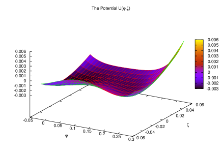
Figure 1: The form of the potential function $U(\varphi,\zeta)$.

For the remaining $a^{0}_{0}$ state the following substitution has been established $a^{0}_{0}\equiv\delta$. The field $\sigma$ describes a broad resonance ($m_{\sigma}\sim 470$ MeV) connected with the exchange of a correlated pair of pions.

II.2 Baryon-meson interaction.

Baryon fields that enter the model are grouped into a $3\times 3$ traceless hermitian matrix

$$B=\left(\begin{array}[]{ccc}\frac{1}{\sqrt{6}}\Lambda+\frac{1}{\sqrt{2}}\Sigma^{0}&\Sigma^{+}&p\\ \Sigma^{-}&\frac{1}{\sqrt{6}}\Lambda-\frac{1}{\sqrt{2}}\Sigma^{0}&n\\ \Xi^{-}&\Xi^{0}&-\frac{2}{\sqrt{6}}\Lambda\\ \end{array}\right).$$ (15)

For the baryon kinetic terms to preserve chiral invariance the local, covariant derivatives have to be used sua ; zschieshce

$$D_{\mu}B=\partial_{\mu}+i[\Gamma_{\mu},B]$$ (16)

where

$$\Gamma_{\mu}=-\frac{i}{2}[u^{\dagger}\partial_{\mu}u+u\partial_{\mu}u^{\dagger}].$$ (17)

and

$$u=exp[\frac{i}{2f_{0}}\pi^{a}\lambda_{a}\gamma_{5}].$$ (18)

Thus the pseudoscalar mesons are given as parameters of the symmetry transformation.
The general form of the baryon($B$) meson ($W$) interaction terms can be written as follows greiner ; sua ; zschieshce

$$\mathcal{L}_{BW}=-\sqrt{2}g_{8}^{W}(\alpha_{W}[\overline{B}\mathcal{O}BW]_{F}+(1-\alpha_{W})[\overline{B}\mathcal{O}BW]_{D})-g_{1}^{W}\frac{1}{\sqrt{3}}Tr(\overline{B}\mathcal{O}B)TrW$$ (19)

where

$$[\overline{B}\mathcal{O}BW]_{F}=Tr(\overline{B}\mathcal{O}WB-\overline{B}\mathcal{O}BW)\\$$ (20)

$$[\overline{B}\mathcal{O}BW]_{D}=Tr(\overline{B}\mathcal{O}WB+\overline{B}\mathcal{O}BW)-\frac{2}{3}Tr(\overline{B}\mathcal{O}B)TrW$$ (21)

The relation (19) it is a mixture of the F-type (antisymmetric) and D-type (symmetric) couplings, $\alpha_{W}$ denotes the $F/F+D$ ratio. The differences for the baryon-scalar and baryon-vector meson interactions are connected with difference in Lorentz space. For scalar mesons $W=\Phi$ and $\mathcal{O}=\textbf{1}$ The masses of the whole baryon multiplet are generated spontaneously by the vacuum expectation value of the nonstrange and strange meson condensates

$$<M>=diag(\frac{\sigma}{\sqrt{2}},\frac{\sigma}{\sqrt{2}},\zeta)$$ (22)

The assumption that $\alpha_{V}=1$ has be made. Setting also $g_{1}^{V}=\sqrt{6}g_{8}^{V}$ the model in which nucleon mass does not depend on the strange condensate is obtained. The value of the nucleon mass can be obtained by adjusting only one coupling constants. The correct values of the remaining baryons it is necessary to introduce an explicit symmetry breaking term.
For the baryon-vector meson interactions $W=V_{\mu}$ and $\mathcal{O}=\gamma_{\mu}$ The universality principle and the vector meson dominance model points to the conclusion that the D-type coupling should be small. Setting as for the case of scalar mesons $\alpha_{V}=1$ and $g_{1}^{V}=\sqrt{6}g_{8}^{V}$, the latter assumption corresponds to the case when strange vector field does not couple to nucleon, the following form of the baryon-vector meson interaction Lagrangian can be written

$$\mathcal{L}_{BV}=-\sqrt{2}g_{8}^{V}([\overline{B}\gamma_{\mu}BV^{\mu}]_{F}+Tr(\overline{B}\gamma_{\mu}B)TrS^{\mu}).$$ (23)

with the singlet vector meson state $S_{\mu}$ and $V_{\mu}$ being the matrix containing the octet of vector meson fields

$$V_{\mu}=\left(\begin{array}[]{ccc}\frac{1}{\sqrt{6}}V_{\mu}^{8}+\frac{1}{\sqrt{2}}\rho^{0}_{\mu}&\rho_{\mu}^{+}&K_{\mu}^{*+}\\ \rho_{\mu}^{-}&\frac{1}{\sqrt{6}}V_{\mu}^{8}-\frac{1}{\sqrt{2}}\rho^{0}_{\mu}&K_{\mu}^{*0}\\ K_{\mu}^{*-}&\bar{K}_{\mu}^{*0}&-\frac{2}{\sqrt{6}}V^{8}_{\mu}\\ \end{array}\right).$$ (24)

The relations for the vector meson couplings reflect quark counting rules.
The physical meson states $\omega$ and $\phi$ are mixed states. They stem from the singlet $S_{\mu}$ and octet $V_{\mu}^{8}$ vector meson states and are given by the relation

$$\omega = V_{\mu}^{8}\cos\theta-S_{\mu}\sin\theta$$ (25)

$$\phi = V_{\mu}^{8}\sin\theta+S_{\mu}\cos\theta.$$

Under the condition that the vector meson $\phi$ is nearly a pure $s\overline{s}$ state as it decays mainly to kaons the mixing with the mixing angle $\tan{\theta}=1/\sqrt{2}$ is called ideal.

II.3 Vector mesons.

The general vector meson Lagrange function can be presented as a sum of the kinetic energy term, mass term and higher order self-interaction terms:

$$\mathcal{L}_{V}=-\frac{1}{4}Tr(V_{\mu\nu}V^{\mu\nu})+\frac{1}{2}m_{V}^{2}Tr(V_{\mu}V^{\mu})-c[Tr(V_{\mu}V^{\mu})^{2}]-dTr[(V^{\mu}V_{\mu})^{2}].$$ (26)

with the field tensor $V_{\mu\nu}=\partial_{\mu}V_{\nu}-\partial_{\nu}V_{\mu}$. This form of the mass term implies a mass degeneracy for the meson nonet.

II.4 Leptons.

Leptons are gathered into $SU_{L}(2)$ dublets and singlets with the flavor $f$ ($f={e,\mu}$)

$$L_{f}=\left(\begin{array}[]{c}\nu_{f}\\ e_{f}\end{array}\right)_{L},\,\,\,e_{fR},\,\,\,\nu_{fR}$$

Assuming that neutrinos $\nu_{f}$ have masses $m_{f}$ the lepton Lagrange function has the form

$$L_{L}=i\overline{L}_{f}\gamma^{\mu}D_{\mu}L_{f}+\overline{e}_{fR}\gamma^{\mu}D_{\mu}e_{fR}-\sum_{f}m_{f}\overline{e}_{f}e_{f}+\sum_{f}i\overline{\nu}_{fL}\gamma^{\mu}D_{\mu}\nu_{fL}+\sum_{f}i\overline{\nu}_{fR}\gamma^{\mu}\partial_{\mu}\nu_{fR}$$

$$-\sum_{f,f^{\prime}}M_{f,f^{\prime}}(\overline{\nu}_{fL}\nu_{f^{\prime}R}+h.c.)-\sum_{f,f^{\prime}}M_{f,f^{\prime}}(\overline{\nu}_{fL}\nu_{f^{\prime}R}+h.c.)$$

The physical massive neutrinos are mixture of neutrinos with different flavors

$$\nu_{fL}=\sum_{i}U_{L,fi}\nu_{iL}$$

$$\nu_{fR}=\sum_{i}U_{R,fi}\nu_{iR}$$

III Relativistic mean field equations.

To investigate the properties of infinite nuclear matter, the mean field approximation has been adopted. The symmetries of infinite nuclear matter simplify the model to a great extent. The translational and rotational invariance claimed that the mean fields of all the vector fields vanish. Only the time-like components of the neutral vector mesons have a non-vanishing expectation value. Owing to parity conservation, the vacuum expectation value of pseudoscalar fields vanish ($<\pi_{a}>=0$). Meson fields have been separated into classical mean field values and quantum fluctuations, which are not included in the ground state. Thus, for the ground state of homogeneous infinite nuclear matter quantum fields operators are replaced by their classical expectation values.

$\sigma=\overline{\sigma}$ +$s_{0}$	$\sigma^{*}=\overline{\sigma}^{*}$ + $s^{*}_{0}$	$\delta^{a}=\overline{\delta}^{a}+d_{0}\delta^{3a}$
$\phi_{\mu}=\overline{\phi}_{\mu}+f_{0}\delta_{\mu 0}$	$\omega_{\mu}=\overline{\omega}_{\mu}+w_{0}\delta_{\mu 0}$	$b_{\mu}^{a}=\overline{b}^{a}_{\mu}+r_{0}\delta_{\mu 0}\delta^{3a}$

When strange hadrons are taken into account uncertainties which are present in the description of nuclear matter are intensified due to the incompleteness of the available experimental data. The standard approach does not reproduce the strongly attractive hyperon-hyperon interaction seen in double $\Lambda$ hypernuclei. In order to construct a proper model which do include hyperons the effects of hyperon-hyperon interactions have to be taken into account. These interactions are simulated via (hidden) strange meson exchange: scalar meson $f_{0}(975)$ ($\sigma^{*}$ meson) and vector meson $\phi(1020)$ ($\phi$ meson) and influence the form of the equation of state and neutron stars properties. The presence of hyperons demands additional coupling constants which have been fitted to hypernuclear properties.
The Lagrangian function for the system is a sum of a baryonic part, including the full octet of baryons, baryon-meson interaction terms, a mesonic part and a free leptonic one. The Lagrangian density of interacting byarons ${\mathcal{L}_{BM}}$ can be explicitly written out in the following form:

$${\mathcal{L}_{BM}}=i\sum_{B}\bar{\psi}_{B}\gamma^{\mu}D_{\mu}\psi_{B}-\sum_{B}\overline{\psi}_{B}M_{eff,B}\psi_{B}$$ (27)

where the spinor $\Psi^{T}=(\psi_{N},\psi_{\Lambda},\psi_{\Sigma},\psi_{\Xi})$ is composed of the following isomultiplets glen ,aqu :

$$\begin{array}[]{cc}\displaystyle\Psi_{N}={\psi_{p}\choose\psi_{n}},&\displaystyle\Psi_{\Lambda}=\psi_{\Lambda},\\ \\ \displaystyle\Psi_{\Sigma}=\left(\begin{array}[]{c}\psi_{\Sigma^{+}}\\ \psi_{\Sigma^{0}}\\ \psi_{\Sigma^{-}}\end{array}\right),&\displaystyle\Psi_{\Xi}={\psi_{\Xi^{0}}\choose\psi_{\Xi^{-}}}.\end{array}$$

$D_{\mu}$ is the covariant derivative given by

$$D_{\mu}=\partial_{\mu}+ig_{\omega B}\omega_{\mu}+ig_{\phi B}\phi_{\mu}+ig_{\rho B}I_{3B}\tau^{a}\rho^{a}_{\mu}.$$ (28)

The meson part of the Lagrangian function includes nonlinear terms that describe additional interactions between mesons.

$$\mathcal{L}_{M}=\frac{1}{2}\partial_{\mu}\sigma\partial^{\mu}\sigma+\frac{1}{2}\partial_{\mu}\delta^{a}\partial^{\mu}\delta^{a}+\frac{1}{2}\partial_{\mu}\sigma^{\ast}\partial^{\mu}\sigma^{\ast}-U_{eff,s}(\sigma,\delta,\sigma^{\ast})$$

$$-\frac{1}{4}\Omega_{\mu\nu}\Omega^{\mu\nu}+\frac{1}{2}M_{\omega}^{2}\omega_{\mu}\omega^{\mu}-\frac{1}{4}R^{a}_{\mu\nu}R^{a\mu\nu}+\frac{1}{2}M_{\rho}^{2}\rho^{a}_{\mu}\rho^{a\mu}$$

$$-\frac{1}{4}\Phi_{\mu\nu}\Phi^{\mu\nu}+\frac{1}{2}M_{\phi}^{2}\phi_{\mu}\phi^{\mu}+U_{eff,v}(\omega,\rho,\phi).$$ (29)

The field tensors $\Omega_{\mu\nu},\Phi_{\mu\nu}$ and $R^{a}_{\mu\nu}$ are defined as

$$\Omega_{\mu\nu}=\partial_{\mu}\omega_{\nu}-\partial_{\nu}\omega_{\mu}\hskip 14.22636pt\Phi_{\mu\nu}=\partial_{\mu}\phi_{\nu}-\partial_{\nu}\phi_{\mu}$$ (30)

$$R^{a}_{\mu\nu}=\partial_{\mu}\rho^{a}_{\nu}-\partial_{\nu}\rho^{a}_{\mu}+g_{\rho}\epsilon_{abc}\rho^{b}_{\mu}\rho^{c}_{\nu}.$$ (31)

All nonlinear meson interaction terms are collected in the vector and scalar potential functions $U_{eff,v}(\omega,\rho,\phi)$ and $U_{eff,s}(\sigma,\delta,\sigma^{\ast})$.
The form of the scalar potential is portrayed by

$$U_{eff,s}(\sigma,\delta,\sigma^{\ast})=\frac{1}{2}m_{\sigma}^{2}\sigma^{2}+\frac{1}{3}g_{2}\sigma^{3}+\frac{1}{4}g_{3}\sigma^{4}+\frac{1}{2}m_{\delta}^{2}(\delta^{a}\delta^{a})$$ (32)

$$+\frac{1}{4}g_{\delta 4}(\delta^{a}\delta^{a})^{2}+g_{\sigma\delta 2}\sigma\delta^{a}\delta^{a}+\frac{1}{2}g_{\sigma 2\delta 2}\sigma^{2}\delta^{a}\delta^{a}$$

$$+\frac{1}{2}m_{\sigma\ast}^{2}\sigma^{\ast 2}+\frac{1}{3}g_{\sigma\ast 3}\sigma^{\ast 3}+\frac{1}{4}g_{\sigma\ast 4}\sigma^{\ast 4}+g_{\sigma\sigma\ast 2}\sigma\sigma^{\ast 2}$$

$$+g_{\sigma\sigma\ast 3}\sigma\sigma^{\ast 3}+g_{\sigma 2\sigma\ast}\sigma^{2}\sigma^{\ast}+g_{\sigma 2\sigma\ast 2}\sigma^{2}\sigma^{\ast 2}+g_{\sigma 3\sigma\ast}\sigma^{3}\sigma^{\ast}$$

$$+g_{\delta 2\sigma\ast}\delta^{2}\sigma^{\ast}+g_{\delta 2\sigma\ast 2}\delta^{2}\sigma^{\ast 2}+g_{\sigma\delta 2\sigma\ast}\sigma\delta^{2}\sigma^{\ast},$$

whereas the effective vector potential has the following form

$$U_{eff,v}(\omega,\rho,\phi)=\frac{1}{4}c_{3}\left((\omega_{\mu}\omega^{\mu})^{2}+(\rho^{a}_{\mu}\rho^{a\mu})^{2}-3(\omega_{\mu}\omega^{\mu}+\rho^{a}_{\mu}\rho^{a\mu})(\phi_{\mu}\phi^{\mu})-(\phi_{\mu}\phi^{\mu})^{2}\right)$$ (33)

The potential function $U_{eff,s}(\sigma,0,0)$ is presented in Fig.2.

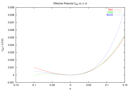
Figure 2: The scalar potential function calculated for different parameter sets.

Scalar potential functions generated for TM1 and GM3 (Glendenning and Moszkowski GM:1991 ) parameter sets are also included in this figure.

Table 1: Parameter sets for chosen equations of state.

	TM1	GM3	SU3
$m_{\sigma}$ (MeV)	511.2	450.0	477.6
$m_{\delta}$ (MeV)	980.0	980.0	1029
$g_{2}$	7.2325 $fm^{-3}$	15.286 $fm^{-3}$	16.196 $fm^{-3}$
$g_{3}$	0.6183	-6.4547	15.669
$g_{\sigma N}=g_{\sigma}$	10.029	7.186	7.923
$g_{\omega}$	12.61	8.702	9.225
$g_{\rho}$	9.264	8.542	5.742
$g_{\sigma\delta 2}$	0	0	32.639 $fm^{-3}$
$g_{\sigma 2\delta 2}$	0	0	29.511
$g_{\delta 4}$	0	0	19.781

Table 2: The nonlinear SU3 parameter set.

$m_{\sigma}$(MeV)	$m_{\delta}$(MeV)	$g_{2}$	$g_{3}$	$g_{\sigma}$
477.6	1029	16.196 $fm^{-3}$	15.669	7.923
$g_{\omega}$	$g_{\rho}$	$g_{\delta 4}$	$g_{\sigma\delta 2}$	$g_{\sigma 2\delta 2}$
9.225	6.754	19.78	31.69 $fm^{-1}$	59.02
$g_{\sigma\ast 3}$	$g_{\delta 2\sigma\ast}$	$g_{\delta 2\sigma\ast 2}$	$g_{\sigma\delta 2\sigma\ast}$	$g_{\sigma\ast 4}$
49.88$fm^{-1}$	-9.51	1.90	21.39	34.07
$g_{\sigma\sigma\ast 2}$	$g_{\sigma\sigma\ast 3}$	$g_{\sigma 2\sigma\ast}$	$g_{\sigma 2\sigma\ast 2}$	$g_{\sigma 3\sigma\ast}$
25.27	12.01	-9.51	1.90	4.88

The scalar $\sigma$ coupling constants for hyperons are chosen to reproduce hyperon potentials in saturated nuclear matter:

$$U_{\Lambda}^{N}(\rho_{0})=-30MeV,\hskip 14.22636ptU_{\Sigma}^{N}(\rho_{0})=+30MeV,\hskip 14.22636ptU_{\Xi}^{N}(\rho_{0})=-18MeV$$ (34)

Upon a recent analysis of $\Sigma^{-}$ atomic data there has been indication of the existence of a repulsive isoscalar potential in the interior of nuclei. This corresponds to a resent search for $\Sigma$ hypernuclei which show the lack of bound-state or continuum peaks. The only found $\Sigma$ bound state is ${}^{4}_{\Sigma}$He. The binding results from the strong isovector component of the $\Sigma$ nuclear interaction. Thus, in the considered model $\Sigma$ hyperons will not appear in the neutron star interior. The experimental data concerning hyperon-hyperon dhsf interaction are extremely scarce. The observed double $\Lambda$ hypernuclear events in emulsion require strong $\Lambda\Lambda$ attractive interaction. An analysis of events which can be interpreted as the creation of $\Lambda\Lambda$ hypernuclei allows us to determine the well depths of hyperon in hyperon matter. The $\sigma^{\ast}$ coupling constants to hyperons, in accordance with the one-boson exchange model D of the Nijmegen group and the measured strong $\Lambda\Lambda$ interaction, are fixed by the condition:

$$-U_{\Xi}^{(\Xi)}\approx-U_{\Lambda}^{(\Xi)}\approx-2U_{\Xi}^{(\Lambda)}\approx-2U_{\Lambda}^{(\Lambda)}\approx 40MeV.$$ (35)

The appropriate parameter set is denoted as SU3 constrained not only by the value of physical scalar meson masses but also by the properties of nuclear matter at saturation. The obtained results are collected in Table 1 and 2.
The effective interaction is introduced through Klain-Gordon equations for the meson fields with baryon densities as source terms. These equations are coupled to the Dirac equations for baryons. All the equations have to be solved self-consistently. The field equations derived from the Lagrange function at the mean field level are the following:

$$(m_{\sigma}^{2}+g_{\sigma 2\delta 2}d_{0}^{2}+g_{\sigma 2\sigma\ast}s_{0}^{\ast})s_{0}+(g_{2}+g_{\sigma 3\sigma\ast}s_{0}^{\ast})s_{0}^{2}+g_{3}s_{0}^{3}$$ (36)

$$=\sum_{B}g_{\sigma B}M^{2}_{eff}S(M_{eff,B})$$

$$m_{\omega}^{2}w_{0}+c_{3}w_{0}^{3}-\frac{3}{2}c_{3}w_{0}f_{0}^{2}=\sum_{B}g_{\omega B}n_{B}$$ (37)

$$m_{\rho}^{2}r_{0}+c_{3}r_{0}^{3}-\frac{3}{2}c_{3}r_{0}f_{0}=\sum_{B}g_{\rho B}I_{3B}n_{B}$$ (38)

$$m_{\delta}^{2}d_{0}^{3}+2(g_{\sigma\delta 2}s_{0}+\frac{1}{2}g_{\sigma 2\delta 2}s_{0}^{2}+\frac{1}{4}g_{\delta 4}+g_{\delta 2\sigma\ast}s_{0}^{\ast}+g_{\delta 2\sigma\ast 2}s_{0}^{\ast 2}+g_{\sigma\delta 2\sigma{\ast}}s_{0}^{\ast}s_{0})d_{0}$$ (39)

$$=\sum_{B}g_{\delta B}I_{3B}S(M_{eff,B})$$

$$m_{\sigma*}^{2}s_{0}^{*}+(g_{\sigma\ast 3}+3g_{\sigma\sigma\ast 3}s_{0})s_{0}^{\ast 2}+g_{\sigma\ast 4}s_{0}^{\ast 3}+2(g_{\sigma\sigma\ast 2}s_{0}+g_{\sigma 2\sigma\ast 2}s_{0}^{2}+g_{\delta 2\sigma\ast 2}d_{0}^{2})s_{0}^{\ast}$$ (40)

$$+(g_{\sigma 2\sigma\ast}s_{0}^{2}+g_{\sigma 3\sigma\ast}s_{0}^{3}+g_{\delta 2\sigma\ast}d_{0}^{2})=\sum_{B}g_{\sigma^{*}B}M^{2}_{eff}S(M_{eff,B})$$

$$m_{\phi}^{2}f_{0}-\frac{3}{2}c_{3}(w_{0}^{2}+r_{0}^{2})f_{0}-c_{3}f_{0}^{3}=\sum_{B}g_{\phi B}n_{B}.$$ (41)

The function $S(M_{eff,B})$ is expressed with the use of the integral

$$S(M_{eff,B})=\frac{2J_{B}+1}{2\pi^{2}}\int_{0}^{\infty}\frac{k^{2}dk}{E(k,M_{eff,B})}(f_{B}-f_{\bar{B}})$$ (42)

where $J_{B}$ and $I_{3B}$ are the spin and isospin projection of baryon $B$, $n_{B}$ which denote the baryon number density is given as

$$n_{B}=\frac{2J_{B}+1}{2\pi^{2}}\int_{0}^{\infty}k^{2}dk(f_{B}-f_{\bar{B}})$$ (43)

The functions $f_{B}$ and $f_{\bar{B}}$ are the Fermi-Dirac distribution for particles and anti-particles respectively

$$f_{B,\bar{B}}=\frac{1}{1+e^{E[(k,M_{eff,B})\mp\mu_{B}]/k_{B}T}}.$$ (44)

The Dirac equation for baryons that is obtained from the Lagrangian function has the following form:

$$(i\gamma^{\mu}\partial_{\mu}-M_{B,eff}-g_{\omega B}\gamma^{0}\omega_{0}-g_{\phi B}\gamma^{0}f_{0}-\frac{1}{2}g_{\rho B}\gamma^{0}\tau^{3}r_{0})\psi=0$$ (45)

from this equation it is noticeable that the baryon develop the effective mass $M_{B,eff}$ generated by the baryon and scalar field interactions and defined as:

$$M_{B,eff}=M_{B}-(g_{\sigma B}s_{0}+g_{\sigma^{*}B}s_{0}^{*}+I_{3B}g_{\delta_{B}}d_{0})$$ (46)

and the effective chemical potential $\mu_{eff}$ is given by

$$\mu_{B,eff}=\mu_{B}-(g_{\omega B}\gamma^{0}\omega_{0}-g_{\phi B}\gamma^{0}f_{0}-\frac{1}{2}g_{\rho B}\gamma^{0}\tau^{3}r_{0})$$ (47)

Numerical solutions of the equation (46) is presented in Fig.3.

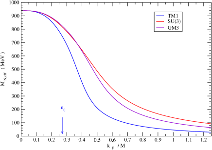
Figure 3: The effective nucleon masses obtained for different parameter sets.

The main effect of the inclusion of $\delta$ meson itself becomes evident when studying properties of neutron star matter especially baryon mass splitting and the form of the equation of state. Fig.3 depicts the effective baryon masses as a function of baryon number density $n_{B}$. There is a noticeable mass splitting of baryons for each isomultiplet in medium which depends on the considered baryonic masses. The bigger is the mass, the smaller the mass differences are. Depending on the sign of the third component of particular baryon isospin the $\delta$ meson interaction increases the proton and $\Xi^{0}$ effective masses and decreases masses of neutron, $\Sigma^{-}$ and $\Xi^{-}$. Contrary to this situation, when $\delta$ meson is not included, the baryon mass for a given isomultiplet remains degenerated. Throughout the effective baryonic masses $\delta$ meson alters baryon chemical potentials what is reflected in characteristic modification of the appearance, abundance and distributions of the individual flavors.

Table 3: Meson-hyperon coupling constants for the ZM1 model.

$g_{\sigma\Lambda}$	0.5207 $g_{\sigma N}$	$g_{\sigma^{\ast}\Lambda}$	0.5815 $g_{\sigma N}$	$g_{\omega\Lambda}$	$\frac{2}{3}$ $g_{\omega N}$
$g_{\rho\Lambda}$	0	$g_{\delta\Lambda}$	0	$g_{\phi\Lambda}$	-$\frac{\sqrt{2}}{3}$ $g_{\omega N}$
$g_{\sigma\Sigma}$	0.1565 $g_{\sigma N}$	$g_{\sigma^{\ast}\Sigma}$	0	$g_{\omega\Sigma}$	$\frac{2}{3}$ $g_{\omega N}$
$g_{\rho\Sigma}$	2 $g_{\rho N}$	$g_{\delta\Sigma}$	2 $g_{\delta N}$	$g_{\phi\Sigma}$	-$\frac{\sqrt{2}}{3}$ $g_{\omega N}$
$g_{\sigma\Xi}$	0.2786 $g_{\sigma N}$	$g_{\sigma^{\ast}\Xi}$	0.5815 $g_{\sigma N}$	$g_{\omega\Xi}$	$\frac{1}{3}$ $g_{\omega N}$
$g_{\rho\Xi}$	$g_{\rho N}$	$g_{\delta\Xi}$	$g_{\delta N}$	$g_{\phi\Xi}$	-$\frac{2\sqrt{2}}{3}$ $g_{\omega N}$

As it was stated earlier neutron star matter possesses highly asymmetric character caused by the presence of small amounts of protons and electrons. The introduction of the asymmetry parameter $f_{a}$ which describes the relative neutron excess defined as

$$f_{a}=\frac{n_{n}-n_{p}}{n_{N}}$$ (48)

allows to study the symmetry properties of the system. Similarly to the asymmetry parameter $f_{a}$ a parameter $f_{s}$ which specify the strangeness content in the system and is strictly connected with the appearance of particular hyperon species in the model has been introduced.

$$f_{s}=\frac{n_{\Lambda}+n_{\Sigma}+2n_{\Xi}}{n_{\Lambda}+n_{\Sigma}+n_{\Xi}+n_{N}}.$$ (49)

IV The derivative coupling model.

The description of the nuclear matter properties with the use of the standard TM1 parameter set reveals a shortcoming which is connected with the appearance of negative nucleon effective masses for densities characteristic for hyperon stars. The Zimanyi-Moszkowski (ZM1) zima model in which the Yukawa type interaction $g_{\sigma N}\sigma$ is replaced by the derivative one $(g_{\sigma N}\sigma/M_{N})\bar{\psi}_{N}\gamma_{\nu}\partial^{\nu}\psi$ exemplifies an alternative version of the Walecka model and improves the behavior of the nucleon effective masses.
In this model in the term which represents the Lagrangian density of interacting baryons is given as follows

$${\mathcal{L}_{BM}}=\sum_{B}(1+\frac{g_{\sigma B}\sigma+g_{\sigma^{*}B}\sigma^{*}+I_{3B}g_{\delta B}\tau^{a}\delta^{a}}{M_{B}})\bar{\psi}_{B}i\gamma^{\mu}D_{\mu}\psi_{B}-\sum_{B}\overline{\psi}_{B}M_{B}\psi_{B}$$ (50)

Rescaling the baryon field in a way proposed by Zimanyi and Moszkowski zima the modified Lagrange function for interacting baryons is obtained

$${\mathcal{L}_{B}}=-\sum_{B}\bar{\psi}_{B}i\gamma^{\mu}D_{\mu}\psi-\sum_{B}\left(1+\frac{g_{\sigma B}\sigma+g_{\sigma^{*}B}\sigma^{*}+I_{3B}g_{\delta B}\tau^{a}\delta^{a}}{M_{B}}\right)^{-1}\overline{\psi}_{B}M_{B}\psi_{B}$$ (51)

Expanding the expression $(1+g_{\sigma N}\sigma/M_{N})^{-1}$ in terms of $g_{sN}\sigma/M_{N}$ (index $N$ denotes nucleons) up to first order in $\sigma$ allows one to reproduce the baryonic part of the Lagrangian of the Walecka model with a Yukawa $N-\sigma$ interaction. The effective baryon mass in this case is given by the following formula

$$M_{B,eff}=\frac{M_{B}}{1+(g_{\sigma B}\sigma+g_{\sigma^{*}B}\sigma^{*}+I_{3B}g_{\delta_{B}}\tau^{a}\delta^{a})/M_{B}}$$ (52)

The parameters employed in the ZM1 model are collected in Tables 3 and 4 bedn2 . In this case the value of the parameter $g_{\rho N}$ has to be redefined in comparison with the standard TM1 value. The parameters $g_{\rho N}$ and $g_{\delta N}$ are adjusted to obtain the symmetry energy coefficient $a_{sym}(n_{0})$ at saturation equal $32.4$ MeV which is in good agreement with the empirical value of about $30\pm 4$ MeV.

Table 4: Meson-nucleon coupling constants for the ZM1 model.

$g_{\sigma N}$	7.84	$g_{\phi N}$	0
$g_{\omega N}$	6.671	$g_{3}$	0
$g_{\rho N}$	9.5	$g_{4}$	0
$g_{\delta N}$	3.1	$c_{3}$	0
$g_{\sigma^{\ast}N}$	0

V Results and conclusions.

On obtaining the form of the equations of state of protoneutron star matter the mass-radius relation and composition of the star can be specified. Two distinctive parameter sets describing strangeness rich matter have been used. The first one denoted as SU3 has been constructed on the basis of chiral symmetry whereas the latter one (ZM1) has been obtained with the use of the derivative coupling model. The considered theories have been extended by the inclusion of $\delta$ meson and nonlinear vector meson interaction terms. The inclusion of $\delta$ meson seems to be indispensable for the complete description of asymmetric neutron star matter. The main effect of the presence of $\delta$ meson becomes evident when studying properties of matter especially baryon mass splitting and the form of the equation of state. Throughout the effective baryon masses $\delta$ meson alters baryon chemical potentials what realizes in characteristic modification of the appearance, abundance and distribution of the individual flavors. The assumptions underlying the calculations performed in this paper are connected with the choice of the repulsive nucleon-hyperon $\Sigma$ interaction.
The forms of the selected equations of state are shown in Fig.4.

Figure 4: The pressure energy density relations for the selected parameter sets.

In agreement with the generally accepted scheme of protoneutron star evolution results for two different cases has been presented. The first one corresponds to the era of neutrino trapping ($Y_{L}=0.4$ and $s=2$) and the second one fulfills the conditions of cold, deleptonized matter ($Y_{L}=0$ and $s=0$). This figure presents also the influence of both entropy and neutrino trapping. For these two cases the SU3 models lead to significantly stiffer equations of state.
In the four successive panels of Fig.5 the analysis of the relative concentrations of particles as functions of baryon number density $n_{B}$ are presented.

Figure 5: The equilibrium composition of protoneutron star matter as a function of the baryon number density $n_{B}$. Upper left panel depicts the composition obtained on the basis of the ZM1 model for $s=2$ and $Y_{l}=0.4$. Upper right has been calculated for $s=0$ and $Y_{l}=0$. Results obtained for SU3 model are presented in lower panels $s=2$ and $Y_{l}=0.4$ (left) and $s=0$ and $Y_{l}=0$(right).

These results indicate that the first strange baryon that emerges is the $\Lambda$ it is followed by $\Xi^{-}$ and $\Xi^{0}$. For both parameter sets the sequence of appearance of hyperons is the same however,in case of ZM1 parameter set, shifted towards higher densities. Due to the repulsive potential of $\Sigma$ hyperons their onset points are possible at very high densities which are not relevant for neutron stars. The appearance of $\Xi^{-}$ hyperons through the condition of charge neutrality affects the electron and muon fractions and causes a drop in their contents. Therefore the appearance of charged hyperons permits the lowering of lepton contents and charge neutrality tends to be guaranteed without lepton contribution. Larger effective baryon masses cause the shift of given hyperon onset point especially for the charged ones in the direction of higher densities.
Any realistic calculation of the properties of neutron stars is based upon the general relativistic equation for hydrostatic equilibrium (the Oppenheimer-Volkoff equation OVT ).
On specifying the equation of state the solution of this equation can be found and this allows us to determine global neutron stars parameters bedn . The structure of spherically symmetric neutron star is determined with the use of this equation which is integrated starting from $\rho=\rho_{c}$ at $r=0$ to the surface at $r=R$ where $\rho=0$. In this way a radius $R$ and a mass $M=m(R)$ for a given central density can be found . As a result, the mass-radius relation can be drown. These relations for the chosen forms of the equations of state are presented in Fig.6. This particular sequence of figures gives a detailed inside into what happens with lowering number of neutrinos ($Y_{\nu}\rightarrow 0$) and decreasing value of entropy. In the left panel of Fig.6 the mass-radius relations for the protoneutron star calculated with the use of ZM1 parameter set is plotted. The right panel depicts the mass-radius relations for SU3 model. In general neutrino trapping increases the value of the maximum mass. The SU3 parameter set gives higher value of the maximum mass then the ZM1 parameter set. Dots which are connected by straight lines represent the evolution of configurations characterized by the same baryon number. In both figures there are configurations which due to deleptonization go to the unstable branch of the neutron star mass-radius relation. The reduction in mass is much bigger in case of the SU3 parameter set.

Figure 6: Deleptonization of a protoneutron star. The left panel presents results obtained for ZM1 parameter set and the right panel for the SU3 model.

The stellar parameters obtained for the maximum mass configuration for different models are presented in Table 5.

model	$M(M_{S}$)	$R(km)$	$\rho_{c}$ ($10^{15}g/cm^{3}$)	$T_{c}$ (MeV)	$P_{c}$ $(MeV/fm^{3})$
SU3, $S=2$, $Y_{L}=0.4$	1.88	12.3	2.0	49.68	268.1
SU3, $T=0$	1.49	10.52	2.43	0.0	189.9
ZM1, $S=2$, $Y_{L}=0.4$	1.62	11.41	2.44	34.88	300.4
ZM1, $T=0$	1.46	11.2	1.98	0.0	166.0

Table 5: Properties of protoneutron maximum mass configurations for SU3 and ZM1 parameter sets.

The solutions of the structure equations also allows us to carry out an analysis of the onset point, abundance and distributions of the individual baryon and lepton species as functions of the star radius. The comparison of results obtained for the two cases presented above (ZM1 and SU(3)) have been made on the basis of the assumption that the repulsive $\Sigma$ interaction shifts the onset point of $\Sigma$ hyperons to very high densities. Consequently, they do not appear in the neutron star interior calculated in these models. The maximum mass configurations has been considered.

Figure 7: The equilibrium composition for the maximum mass configuration as functions of the stellar radius $R$. Upper left panel depicts the composition obtained on the basis of the ZM1 model for $s=2$ and $Y_{l}=0.4$. Upper right has been calculated for $s=0$. Results obtained for SU3 model are presented in lower panels $s=2$ and $Y_{l}=0.4$ (left) and $s=0$ (right).

In case of trapped neutrinos the ZM1 model leads to more compact strangeness rich core. This very compact hyperon core which emerges in the interior of the maximum mass configuration consists of $\Xi^{-}$ and $\Lambda$ hyperons as shown in the upper left panel of Fig.7. The presence of negatively charged hyperons reduces the content of negatively charged leptons. For the SU3 model the strangeness rich core is more extended (the bottom left of Fig.7) but in case of neutrino trapped matter it contains only $\Lambda$ hyperon. The absence of negatively charged hyperons leaves the electron and muon content unchanged. After deleptonization the strangeness rich core in case of the SU3 model remains more extended than in the case of ZM1 parameter set but it contains $\Xi^{0}$, $\Xi^{-}$ and $\Lambda$ hyperons.
The relative baryon composition in this model can be also analyzed through the density dependence of the asymmetry parameter $f_{a}$ and the strangeness contents $f_{s}$. Fig.8 presents both parameters as functions of the star radius $R$.

Figure 8: The asymmetry parameter $f_{a}$ (the left panel) and the strangeness content parameter $f_{s}$ (the right panel) as functions of the stellar radius $R$ .

As it was shown in Fig.7 trapped neutrinos have an influence on the charged hyperon onset points. The appearance of additional negatively charged particles has the consequence on the proton content in the system and this in turn on the asymmetry parameter $f_{a}$.
Fig. 9 depict the relative fractions of protons, electrons and muons for the ZM1 and SU3 parameter sets.

Figure 9: Electron (left panel)and proton and neutrino (right panel) fractions $Y_{i}$, as functions of baryon number density $n_{B}$.

Fig. 8 compares the asymmetry parameter $f_{a}$ for ZM1 and the SU3 parameter sets. It is noticeable that SU3 parameters give less asymmetric protoneutron and neutron star but with the higher value of the strangeness content parameter $f_{s}$.
Fig. 10 depicts the temperature profiles plotted for the presented above models.

Figure 10: Stellar temperature as a function of the star radius.

In case of ZM1 protoneutron star model the temperature in interior of maximum mass configuration takes higher value than in case of SU3 model. The appearance of the strangeness-rich core on both plots is marked by the local inversion of temperature.

References

- (1) Aguirre R., De Paoli A.L. 2002 Eur.Phys.J. textbfA13, 501
- (2) Bednarek I., Manka R. 2001 Int. Journal Mod. Phys. D10, 607
- (3) Bednarek I., Keska M.,Manka R. 2003 Phys. Rev. C68, 035805
- (4) Bodmer A.R., 1991, Nucl.Phys., A526, 703
- (5) J. Boguta and A.R. Bodmer, 1977, Nucl. Phys., A292 413, Int. J. Mod. Phys., E6, 515
- (6) Burrows A., Lattimer J.M. 1986Astrophys. J. 307 178
- (7) Gasiorowicz S., Geffen D.A., 1969, Rev. Mod. Phys., 41, 531
- (8) Glendenning N.K., Astrophys.J., 293, 470 (1985); Also see in Compact Stars by N. K Glendenning Sringer-Verlag, New York (1997)
- (9) N.K. Glendenning and S.A. Moszkowski, 1991, Phys. Rev. Lett., 67, 2414
- (10) Greiner C., Schaffner-Biellich J., nucl-th/9801062
- (11) Kubis S., Kutschera M., 1997, Phys. Lett. B399 191
- (12) Lattimer J.M., Prakash M. 2001 Astrophys. J.550 426
- (13) Papazoglou P., Zschiesche D., Schramm S., Schaffner-Bielich J., Stöcker H., Greiner W., 1998, Phys. Rev.,C59,411,Papazoglou P.,Schramm S., Schaffner-Bielich j., Stöcker H., Greiner W., 1998, Phys. Rev., C57, 2576, Hanauske M., Zschiesche D., Pal S., Schramm S., Stöcker H., Greiner W.,2000,Ap.J.,573,958
- (14) Pons J.A., Reddy S., Ellis P.J., Prakash M., Lattimer J.M. Phys. Rev.C 62 035803
- (15) Prakash M., Bombaci I., Manju Prakash, Ellis P.J., Lattimer J.M., Knorren R. 1997 Phys. Rep. 280 1
- (16) Reinhard P.-G., Rufa M. , Maruhn J., Greiner W. and Friedrich J. 1986 Z. Phys. A - Atomic Nuclei323 13
- (17) J. Schaffner and I.N. Mishustin, 1996, Phys. Rev., C53, 1416
- (18) Serot B.D., Walecka J.D. 1986 Adv. Nucl. Phys. 16 1; 1997 Int. J. Mod. Phys. E6 515
- (19) Sugahara Y. and Toki H. 1994 Prog. Theo. Phys 92 803
- (20) R. C. Tolman, 1939, Phys. Rev., 55, 364; J.R. Oppenheimer and G.M. Volkoff, 1939, Phys. Rev., 55, 374
- (21) Törnqvist N.A., 1997, The linear U(3) U(3) sigma model, the sigma (500) and the spontaneous breaking of symmetries, hep-ph/9711483
- (22) Weber F. Pulsars as Astrophysical Laboratories for Nuclear and Particle Physics, 1999, IOP Publishing, Philadelphia
- (23) Zimanyi J., Moszkowski S.A., 1990, Phys. Rev. C42 1416
- (24) Zschiesche D., Mishira A., Schramm S., Stöcker H., Greiner W., nucl-th/0302073