Spin polarized states in nuclear matter
with Skyrme effective interaction

Abstract

The possibility of appearance of spin polarized states in symmetric and strongly asymmetric nuclear matter is analyzed within the framework of a Fermi liquid theory with the Skyrme effective interaction. The zero temperature dependence of the neutron and proton spin polarization parameters as functions of density is found for SkM^∗, SGII (symmetric case) and SLy4, SLy5 (strongly asymmetric case) effective forces. By comparing free energy densities, it is shown that in symmetric nuclear matter ferromagnetic spin state (parallel orientation of neutron and proton spins) is more preferable than antiferromagnetic one (antiparallel orientation of spins). Strongly asymmetric nuclear matter undergoes at some critical density a phase transition to the state with the oppositely directed spins of neutrons and protons while the state with the same direction of spins does not appear. In comparison with neutron matter, even small admixture of protons strongly decreases the threshold density of spin instability. It is clarified that protons become totally polarized within a very narrow density domain while the density profile of the neutron spin polarization parameter is characterized by the appearance of long tails near the transition density.

I Introduction

The spontaneous appearance of spin polarized states in nuclear matter is the topic of a great current interest due to relevance in astrophysics. In particular, the effects of spin correlations in the medium strongly influence the neutrino cross section and neutrino luminosity. Hence, depending on whether nuclear matter is spin polarized or not, drastically different scenarios of supernova explosion and cooling of neutron stars can be realized. Another aspect relates to pulsars, which are considered to be rapidly rotating neutron stars, surrounded by strong magnetic field. There is still no general consensus regarding the mechanism to generate such strong magnetic field of a neutron star. One of the hypotheses is that magnetic field can be produced by a spontaneous ordering of spins in the dense stellar core.

The possibility of a phase transition of normal nuclear matter to the ferromagnetic state was studied by many authors. In the gas model of hard spheres, neutron matter becomes ferromagnetic at $\varrho\approx 0.41\,\mbox{fm}^{-3}$ R . It was found in Refs. S ; O that the inclusion of long–range attraction significantly increases the ferromagnetic transition density (e.g., up to $\varrho\approx 2.3\,\mbox{fm}^{-3}$ in the Brueckner theory with a simple central potential and hard core only for singlet spin states O ). By determining magnetic susceptibility with Skyrme effective forces, it was shown in Ref. VNB that the ferromagnetic transition occurs at $\varrho\approx 0.18$–$0.26\,\mbox{fm}^{-3}$. The Fermi liquid criterion for the ferromagnetic instability in neutron matter with the Skyrme interaction is reached at $\varrho\approx 2$–$4\varrho_{0}$ RPLP , where $\varrho_{0}=0.16\,\mbox{fm}^{-3}$ is the nuclear matter saturation density. The general conditions on the parameters of neutron–neutron interaction, which result in a magnetically ordered state of neutron matter, were formulated in Ref. ALP . Spin correlations in dense neutron matter were studied within the relativistic Dirac–Hartree–Fock approach with the effective nucleon–meson Lagrangian in Ref. MNQN , predicting the ferromagnetic transition at several times nuclear matter saturation density. The importance of the Fock exchange term in the relativistic mean–field approach for the occurrence of ferromagnetism in nuclear matter was established in Ref. TT . The stability of strongly asymmetric nuclear matter with respect to spin fluctuations was investigated in Ref. KW , where it was shown that the system with localized protons can develop a spontaneous polarization, if the neutron–proton spin interaction exceeds some threshold value. This conclusion was confirmed also by calculations within the relativistic Dirac–Hartree–Fock approach to strongly asymmetric nuclear matter BMNQ .

For the models with realistic nucleon–nucleon (NN) interaction, the ferromagnetic phase transition seems to be suppressed up to densities well above $\varrho_{0}$ PGS –H . In particular, no evidence of ferromagnetic instability has been found in recent studies of neutron matter VPR and asymmetric nuclear matter VB within the Brueckner–Hartree–Fock approximation with realistic Nijmegen II, Reid93 and Nijmegen NSC97e NN interactions. The same conclusion was obtained in Ref. FSS , where magnetic susceptibility of neutron matter was calculated with the use of the Argonne $v_{18}$ two–body potential and Urbana IX three–body potential.

Here we continue the study of spin polarizability of nuclear matter with the use of an effective NN interaction. As a framework of consideration, a Fermi liquid (FL) description of nuclear matter is chosen AKP ; AIP . As a potential of NN interaction, we use the Skyrme effective interaction, utilized earlier in a number of contexts for nuclear matter calculations SYK –AAI . We explore the possibility of FM and AFM phase transitions in nuclear matter, when the spins of protons and neutrons are aligned in the same direction or in the opposite direction, respectively. In contrast to the approach, based on the calculation of magnetic susceptibility, we obtain the self–consistent equations for the FM and AFM spin order parameters and find their solutions at zero temperature. This allows us to determine not only the critical density of instability with respect to spin fluctuations, but also to establish the density dependence of the order parameters and to clarify the question of thermodynamic stability of various phases. The main emphasis in our study will be laid on the region of zero isospin asymmetry (symmetric nuclear matter) and large isospin asymmetry (strongly asymmetric nuclear matter and neutron matter).

Note that we consider the thermodynamic properties of spin polarized states in nuclear matter up to the high density region relevant for astrophysics. Nevertheless, we take into account the nucleon degrees of freedom only, although other degrees of freedom, such as pions, hyperons, kaons, or quarks could be important at such high densities.

II Basic Equations

The normal states of nuclear matter are described by the normal distribution function of nucleons $f_{\kappa_{1}\kappa_{2}}=\mbox{Tr}\,\varrho a^{+}_{\kappa_{2}}a_{\kappa_{1}}$, where $\kappa\equiv({\bf{p}},\sigma,\tau)$, ${\bf p}$ is momentum, $\sigma(\tau)$ is the projection of spin (isospin) on the third axis, and $\varrho$ is the density matrix of the system I ; IY . The energy of the system is specified as a functional of the distribution function $f$, $E=E(f)$, and determines the single particle energy

$$\varepsilon_{\kappa_{1}\kappa_{2}}(f)=\frac{\partial E(f)}{\partial f_{\kappa_{2}\kappa_{1}}}.$$ (1)

The self-consistent matrix equation for determining the distribution function $f$ follows from the minimum condition of the thermodynamic potential and is

$$f=\left\{\mbox{exp}(Y_{0}\varepsilon+Y_{4})+1\right\}^{-1}\equiv\left\{\mbox{exp}(Y_{0}\xi)+1\right\}^{-1}.$$ (2)

Here the quantities $\varepsilon$ and $Y_{4}$ are matrices in the space of $\kappa$ variables, with $Y_{4\kappa_{1}\kappa_{2}}=Y_{4\tau_{1}}\delta_{\kappa_{1}\kappa_{2}}$ $(\tau_{1}=n,p)$, $Y_{0}=1/T,\ Y_{4n}=-\mu_{n}^{0}/T$ and $Y_{4p}=-\mu_{p}^{0}/T$ being the Lagrange multipliers, $\mu_{n}^{0}$ and $\mu_{p}^{0}$ the chemical potentials of neutrons and protons, and $T$ the temperature. Since it is assumed to consider a nuclear system with an excess of neutrons, the positive isospin projection is assigned to neutrons. Further we shall study the possibility of formation of various types of spin ordering (with parallel and antiparallel orientation of neutron and proton spins) in nuclear matter.

The normal distribution function can be expanded in the Pauli matrices $\sigma_{i}$ and $\tau_{k}$ in spin and isospin spaces

$$f({\bf p}) =f_{00}({\bf p})\sigma_{0}\tau_{0}+f_{30}({\bf p})\sigma_{3}\tau_{0}$$ (3)

$$\quad+f_{03}({\bf p})\sigma_{0}\tau_{3}+f_{33}({\bf p})\sigma_{3}\tau_{3}.$$

For the energy functional invariant with respect to rotations in spin and isospin spaces, the structure of the single particle energy is similar to the structure of the distribution function $f$:

$$\varepsilon({\bf p}) =\varepsilon_{00}({\bf p})\sigma_{0}\tau_{0}+\varepsilon_{30}({\bf p})\sigma_{3}\tau_{0}$$ (4)

$$\quad+\varepsilon_{03}({\bf p})\sigma_{0}\tau_{3}+\varepsilon_{33}({\bf p})\sigma_{3}\tau_{3}.$$

Using Eqs. (2) and (4), one can express evidently the distribution functions $f_{00},f_{30},f_{03},f_{33}$ in terms of the quantities $\varepsilon$:

$$f_{00} =\frac{1}{4}\{n(\omega_{+,+})+n(\omega_{+,-})+n(\omega_{-,+})+n(\omega_{-,-})\},$$

$$f_{30} =\frac{1}{4}\{n(\omega_{+,+})+n(\omega_{+,-})-n(\omega_{-,+})-n(\omega_{-,-})\},$$

$$f_{03} =\frac{1}{4}\{n(\omega_{+,+})-n(\omega_{+,-})+n(\omega_{-,+})-n(\omega_{-,-})\},$$

$$f_{33} =\frac{1}{4}\{n(\omega_{+,+})-n(\omega_{+,-})-n(\omega_{-,+})+n(\omega_{-,-})\}.$$ (5)

Here $n(\omega)=\{\exp(Y_{0}\omega)+1\}^{-1}$ and

$$\omega_{+,+}=\xi_{00}+\xi_{30}+\xi_{03}+\xi_{33},\;$$

$$\omega_{+,-}=\xi_{00}+\xi_{30}-\xi_{03}-\xi_{33},\;$$

$$\omega_{-,+}=\xi_{00}-\xi_{30}+\xi_{03}-\xi_{33},\;$$

$$\omega_{-,-}=\xi_{00}-\xi_{30}-\xi_{03}+\xi_{33},\;$$

where

$$\xi_{00} =\varepsilon_{00}-\mu_{00}^{0},\;\xi_{30}=\varepsilon_{30},\;$$

$$\xi_{03} =\varepsilon_{03}-\mu_{03}^{0},\;\xi_{33}=\varepsilon_{33},$$

$$\mu_{00}^{0} ={\frac{\mu_{n}^{0}+\mu_{p}^{0}}{2}},\quad\mu_{03}^{0}={\frac{\mu_{n}^{0}-\mu_{p}^{0}}{2}}.$$

As follows from the structure of the distribution functions $f$, the quantity $\omega_{\pm,\pm}$, being the exponent in the Fermi distribution function $n$, plays the role of the quasiparticle spectrum. We consider the case when the spectrum is fourfold split due to the spin and isospin dependence of the single particle energy $\varepsilon({\bf p})$ in Eq. (4). The branches $\omega_{\pm,+}$ correspond to neutrons with spin up and spin down, and the branches $\omega_{\pm,-}$ correspond to protons with spin up and spin down.

The distribution functions $f$ should satisfy the normalization conditions

$$\frac{4}{\cal V}\sum_{\bf p}f_{00}({\bf p}) =\varrho,$$ (6)

$$\frac{4}{\cal V}\sum_{\bf p}f_{03}({\bf p}) =\varrho_{n}-\varrho_{p}\equiv\alpha\varrho,$$ (7)

$$\frac{4}{\cal V}\sum_{\bf p}f_{30}({\bf p}) =\varrho_{\uparrow}-\varrho_{\downarrow}\equiv\Delta\varrho_{\uparrow\uparrow},$$ (8)

$$\frac{4}{\cal V}\sum_{\bf p}f_{33}({\bf p}) =(\varrho_{n\uparrow}+\varrho_{p\downarrow})-(\varrho_{n\downarrow}+\varrho_{p\uparrow})\equiv\Delta\varrho_{\uparrow\downarrow}.$$ (9)

Here $\alpha$ is the isospin asymmetry parameter, $\varrho_{n\uparrow},\varrho_{n\downarrow}$ and $\varrho_{p\uparrow},\varrho_{p\downarrow}$ are the neutron and proton number densities with spin up and spin down, respectively; $\varrho_{\uparrow}=\varrho_{n\uparrow}+\varrho_{p\uparrow}$ and $\varrho_{\downarrow}=\varrho_{n\downarrow}+\varrho_{p\downarrow}$ are the nucleon densities with spin up and spin down. The quantities $\Delta\varrho_{\uparrow\uparrow}$ and $\Delta\varrho_{\uparrow\downarrow}$ may be regarded as FM and AFM spin order parameters. Indeed, in symmetric nuclear matter, if all nucleon spins are aligned in one direction (totally polarized FM spin state), then $\Delta\varrho_{\uparrow\uparrow}=\varrho$ and $\Delta\varrho_{\uparrow\downarrow}=0$; if all neutron spins are aligned in one direction and all proton spins in the opposite one (totally polarized AFM spin state), then $\Delta\varrho_{\uparrow\downarrow}=\varrho$ and $\Delta\varrho_{\uparrow\uparrow}=0$. In turn, from Eqs. (6)–(9) one can find the neutron and proton number densities with spin up and spin down as functions of the total density $\varrho$, isospin excess $\delta\varrho\equiv\alpha\varrho$, and FM and AFM order parameters $\Delta\varrho_{\uparrow\uparrow}$ and $\Delta\varrho_{\uparrow\downarrow}$:

$$\varrho_{n\uparrow} =\frac{1}{4}(\varrho+\delta\varrho+\Delta\varrho_{\uparrow\uparrow}+\Delta\varrho_{\uparrow\downarrow}),$$

$$\varrho_{n\downarrow} =\frac{1}{4}(\varrho+\delta\varrho-\Delta\varrho_{\uparrow\uparrow}-\Delta\varrho_{\uparrow\downarrow}),$$

$$\varrho_{p\uparrow} =\frac{1}{4}(\varrho-\delta\varrho+\Delta\varrho_{\uparrow\uparrow}-\Delta\varrho_{\uparrow\downarrow}),$$

$$\varrho_{p\downarrow} =\frac{1}{4}(\varrho-\delta\varrho-\Delta\varrho_{\uparrow\uparrow}+\Delta\varrho_{\uparrow\downarrow}).$$

In order to characterize spin ordering in the neutron and proton subsystems, it is convenient to introduce neutron and proton spin polarization parameters

$$\Pi_{n}=\frac{\varrho_{n\uparrow}-\varrho_{n\downarrow}}{\varrho_{n}},\quad\Pi_{p}=\frac{\varrho_{p\uparrow}-\varrho_{p\downarrow}}{\varrho_{p}}.$$ (10)

The expressions for the spin order parameters $\Delta\varrho_{\uparrow\uparrow}$ and $\Delta\varrho_{\uparrow\downarrow}$ through the spin polarization parameters read

$$\Delta\varrho_{\uparrow\uparrow}=\varrho_{n}\Pi_{n}+\varrho_{p}\Pi_{p},\;\Delta\varrho_{\uparrow\downarrow}=\varrho_{n}\Pi_{n}-\varrho_{p}\Pi_{p}.$$

To obtain the self–consistent equations, we specify the energy functional of the system in the form

$$E(f) =E_{0}(f)+E_{int}(f),$$ (11)

$${E}_{0}(f) =4\sum\limits_{\bf p}\varepsilon_{0}({\bf p})f_{00}({\bf p}),\;\varepsilon_{0}({\bf p})=\frac{{\bf p}^{\,2}}{2m_{0}},$$ (12)

$${E}_{int}(f) =2\sum\limits_{\bf p}\{\tilde{\varepsilon}_{00}({\bf p})f_{00}({\bf p})+\tilde{\varepsilon}_{30}({\bf p})f_{30}({\bf p})$$ (13)

$$\quad+\tilde{\varepsilon}_{03}({\bf p})f_{03}({\bf p})+\tilde{\varepsilon}_{33}({\bf p})f_{33}({\bf p})\},$$

$$\tilde{\varepsilon}_{00}({\bf p}) =\frac{1}{2\cal V}\sum_{\bf q}U_{0}({\bf k})f_{00}({\bf q}),\;{\bf k}=\frac{{\bf p}-{\bf q}}{2},$$

$$\tilde{\varepsilon}_{30}({\bf p}) =\frac{1}{2\cal V}\sum_{\bf q}U_{1}({\bf k})f_{30}({\bf q}),$$

$$\tilde{\varepsilon}_{03}({\bf p}) =\frac{1}{2\cal V}\sum_{\bf q}U_{2}({\bf k})f_{03}({\bf q}),$$

$$\tilde{\varepsilon}_{33}({\bf p}) =\frac{1}{2\cal V}\sum_{\bf q}U_{3}({\bf k})f_{33}({\bf q}).$$

Here $m_{0}$ is the bare mass of a nucleon, $U_{0}({\bf k}),...,U_{3}({\bf k})$ are the normal FL amplitudes, and $\tilde{\varepsilon}_{00},\tilde{\varepsilon}_{30},\tilde{\varepsilon}_{03},\tilde{\varepsilon}_{33}$ are the FL corrections to the free single particle spectrum. Further we do not take into account the effective tensor forces, which lead to coupling of the momentum and spin degrees of freedom HJ ; D ; FMS , and, correspondingly, to anisotropy in the momentum dependence of FL amplitudes with respect to the spin polarization axis. Using Eqs. (1) and (11), we get the self–consistent equations in the form

$$\xi_{00}({\bf p}) =\varepsilon_{0}({\bf p})+\tilde{\varepsilon}_{00}({\bf p})-\mu_{00}^{0},\;\xi_{30}({\bf p})=\tilde{\varepsilon}_{30}({\bf p}),$$ (14)

$$\xi_{03}({\bf p}) =\tilde{\varepsilon}_{03}({\bf p})-\mu_{03}^{0},\;\xi_{33}({\bf p})=\tilde{\varepsilon}_{33}({\bf p}).$$

To obtain numerical results, we use the Skyrme effective interaction. In the case of Skyrme forces the normal FL amplitudes read

$$U_{0}({\bf k}) =6t_{0}+t_{3}\varrho^{\beta}+\frac{2}{\hbar^{2}}[3t_{1}+t_{2}(5+4x_{2})]{\bf k}^{2},$$ (15)

$$U_{1}({\bf k}) =-2t_{0}(1-2x_{0})-\frac{1}{3}t_{3}\varrho^{\beta}(1-2x_{3})$$

$$\quad-\frac{2}{\hbar^{2}}[t_{1}(1-2x_{1})-t_{2}(1+2x_{2})]{\bf k}^{2}\equiv a+b{\bf k}^{2},$$

$$U_{2}({\bf k}) =-2t_{0}(1+2x_{0})-\frac{1}{3}t_{3}\varrho^{\beta}(1+2x_{3})$$

$$\quad-\frac{2}{\hbar^{2}}[t_{1}(1+2x_{1})-t_{2}(1+2x_{2})]{\bf k}^{2},$$

$$U_{3}({\bf k}) =-2t_{0}-\frac{1}{3}t_{3}\varrho^{\beta}-\frac{2}{\hbar^{2}}(t_{1}-t_{2}){\bf k}^{2}\equiv c+d{\bf k}^{2},$$

where $t_{i},x_{i},\beta$ are the phenomenological constants, characterizing a given parametrization of the Skyrme forces. Eqs. (15) are derived in Appendix. In the numerical calculations we shall use SkM^∗ BGH and SGII SG potentials, designed for describing the properties of systems with small isospin asymmetry, and SLy4 and SLy5 potentials CBH , developed to fit the properties of systems with large isospin asymmetry. With account of the evident form of FL amplitudes and Eqs. (6)–(9), one can obtain

$$\xi_{00} =\frac{p^{2}}{2m_{00}}-\mu_{00},$$ (16)

$$\xi_{03} =\frac{p^{2}}{2m_{03}}-\mu_{03},$$ (17)

$$\xi_{30} =(a+b\frac{{\bf p}^{2}}{4})\frac{\Delta\varrho_{\uparrow\uparrow}}{8}+\frac{b}{32}\langle{\bf q}^{2}\rangle_{30},$$ (18)

$$\xi_{33} =(c+d\frac{{\bf p}^{2}}{4})\frac{\Delta\varrho_{\uparrow\downarrow}}{8}+\frac{d}{32}\langle{\bf q}^{2}\rangle_{33},$$ (19)

where the effective nucleon mass $m_{00}$ and effective isovector mass $m_{03}$ are defined by the formulae:

$$\frac{\hbar^{2}}{2m_{00}} = \frac{\hbar^{2}}{2m_{0}}+\frac{\varrho}{16}[3t_{1}+t_{2}(5+4x_{2})],$$ (20)

$$\frac{\hbar^{2}}{2m_{03}} = \frac{\alpha\varrho}{16}[t_{2}(1+2x_{2})-t_{1}(1+2x_{1})],$$

and the renormalized chemical potentials $\mu_{00}$ and $\mu_{03}$ should be determined from Eqs. (6) and (7). In Eqs.  (18) and (19), $\langle{\bf q}^{2}\rangle_{30}$ and $\langle{\bf q}^{2}\rangle_{33}$ are the second order moments of the corresponding distribution functions

$$\langle{\bf q}^{2}\rangle_{30} =\frac{4}{V}\sum_{\bf q}{\bf q}^{2}f_{30}({\bf q}),$$ (21)

$$\langle{\bf q}^{2}\rangle_{33} =\frac{4}{V}\sum_{\bf q}{\bf q}^{2}f_{33}({\bf q}).$$ (22)

Thus, with account of expressions (5) for the distribution functions $f$, we obtain the self–consistent equations (6)–(9), (21), and (22) for the effective chemical potentials $\mu_{00},\mu_{03}$, FM and AFM spin order parameters $\Delta\varrho_{\uparrow\uparrow}$, $\Delta\varrho_{\uparrow\downarrow}$, and second order moments $\langle{\bf q}^{2}\rangle_{30},\langle{\bf q}^{2}\rangle_{33}$. It is easy to see, that the self–consistent equations remain invariable under a global flip of spins, when neutrons (protons) with spin up and spin down are interchanged, and under a global flip of isospins, when neutrons and protons with the same spin projection are interchanged.

Let us consider, what differences will be in the case of neutron matter. Neutron matter is an infinite nuclear system, consisting of nucleons of one species, i.e., neutrons, and, hence, the formalism of one–component Fermi liquid should be applied for the description of its properties. Formally neutron matter can be considered as the limiting case of asymmetric nuclear matter, corresponding to the isospin asymmetry $\alpha=1$. The individual state of a neutron is characterized by momentum $\bf p$ and spin projection $\sigma$. The self–consistent equation has the form of Eq. (2), where all quantities are matrices in the space of $\kappa\equiv(\textbf{p},\sigma)$ variables. The normal distribution function and single particle energy can be expanded in the Pauli matrices in spin space

$$f({\bf p}) =f_{0}({\bf p})\sigma_{0}+f_{3}({\bf p})\sigma_{3},$$ (23)

$$\varepsilon({\bf p}) =\varepsilon_{0}({\bf p})\sigma_{0}+\varepsilon_{3}({\bf p})\sigma_{3}.$$

The energy functional of neutron matter is characterized by two normal FL amplitudes $U_{0}^{n}(\textbf{k})$ and $U_{1}^{n}(\textbf{k})$. The normal FL amplitudes can be found in terms of the Skyrme force parameters $t_{i},x_{i},\beta$ (the details of the derivation procedure are given in Appendix):

$$U_{0}^{n}({\bf k}) =2t_{0}(1-x_{0})+\frac{t_{3}}{3}\varrho^{\beta}(1-x_{3})$$ (24)

$$\quad+\frac{2}{\hbar^{2}}[t_{1}(1-x_{1})+3t_{2}(1+x_{2})]{\bf k}^{2},$$

$$U_{1}^{n}({\bf k}) =-2t_{0}(1-x_{0})-\frac{t_{3}}{3}\varrho^{\beta}(1-x_{3})$$ (25)

$$\quad+\frac{2}{\hbar^{2}}[t_{2}(1+x_{2})-t_{1}(1-x_{1})]{\bf k}^{2}\equiv a_{n}+b_{n}{\bf k}^{2}.$$

With account of Eqs. (24) and (25), the normalization conditions for the distribution functions can be written in the form

$$\frac{2}{\cal V}\sum_{\bf p}f_{0}({\bf p}) =\varrho,\;$$ (26)

$$\frac{2}{\cal V}\sum_{\bf p}f_{3}({\bf p}) =\varrho_{\uparrow}-\varrho_{\downarrow}\equiv\Delta\varrho_{\uparrow\uparrow}.$$ (27)

Here $\varrho_{\uparrow}$ and $\varrho_{\downarrow}$ are the neutron number densities with spin up and spin down and

$$f_{0} =\frac{1}{2}\{n(\omega_{+})+n(\omega_{-})\},\quad\omega_{\pm}=\xi_{0}\pm\xi_{3},$$ (28)

$$f_{3} =\frac{1}{2}\{n(\omega_{+})-n(\omega_{-})\},$$ (29)

$$\xi_{0} =\frac{p^{2}}{2m_{n}}-\mu_{n},$$ (30)

$$\xi_{3} =(a_{n}+b_{n}\frac{{\bf p}^{2}}{4})\frac{\Delta\varrho_{\uparrow\uparrow}}{4}+\frac{b_{n}}{16}\langle{\bf q}^{2}\rangle_{3}.$$ (31)

The effective neutron mass $m_{n}$ is defined by the formula

$$\frac{\hbar^{2}}{2m_{n}} = \frac{\hbar^{2}}{2m_{0}}+\frac{\varrho}{8}[t_{1}(1-x_{1})+3t_{2}(1+x_{2})],$$ (32)

and the quantity $\langle{\bf q}^{2}\rangle_{3}$ in Eq. (31) is the second order moment of the distribution function $f_{3}$:

$$\langle{\bf q}^{2}\rangle_{3} =\frac{2}{V}\sum_{\bf q}{\bf q}^{2}f_{3}({\bf q}).$$ (33)

Thus, with account of expressions (28) and (29) for the distribution functions $f$, we obtain the self–consistent equations (26), (27), and (33) for the effective chemical potential $\mu_{n}$, spin order parameter $\Delta\varrho_{\uparrow\uparrow}$, and second order moment $\langle{\bf q}^{2}\rangle_{3}$.

III Phase transitions in symmetric nuclear matter

Early research on spin polarizability of nuclear matter with the Skyrme effective interaction were based on the calculation of magnetic susceptibility and finding its pole structure VNB ; RPLP , determining the onset of instability with respect to spin fluctuations. Here we shall find directly solutions of the self–consistent equations for the FM and AFM spin order parameters as functions of density at zero temperature. In this section a special emphasis will be laid on the study of symmetric nuclear matter ($\alpha=0$), while in the next section on the investigation of strongly asymmetric nuclear matter ($\alpha\lesssim 1$), including neutron matter as its limiting case.

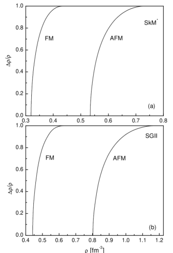
Figure 1: FM and AFM spin polarization parameters as functions of density at zero temperature for (a) SkM^∗ force and (b) SGII force.

Let us consider the zero temperature behavior of spin polarization in symmetric nuclear matter ($\varrho_{p}=\varrho_{n}$). The FM spin ordering corresponds to the case $\Delta\varrho_{\uparrow\uparrow}\not=0,\langle{\bf q}^{2}\rangle_{30}\not=0,\Delta\varrho_{\uparrow\downarrow}=0,\langle{\bf q}^{2}\rangle_{33}=0$, while the AFM spin ordering to the case $\Delta\varrho_{\uparrow\downarrow}\not=0,\langle{\bf q}^{2}\rangle_{33}\not=0,\Delta\varrho_{\uparrow\uparrow}=0,\langle{\bf q}^{2}\rangle_{30}=0$. In the totally ferromagnetically polarized state nontrivial solutions of the self–consistent equations have the form

$$\Delta\varrho_{\uparrow\uparrow}=\varrho,\;\langle{\bf q}^{2}\rangle_{30}=\frac{3}{5}\varrho k_{F}^{2}.$$ (34)

Here $k_{F}=(3\pi^{2}\varrho)^{1/3}$ is Fermi momentum of symmetric nuclear matter in the case when degrees of freedom, corresponding to spin up of nucleons, are open while those related to spin down are inaccessible. For the totally antiferromagnetically polarized nuclear matter we have

$$\Delta\varrho_{\uparrow\downarrow}=\varrho,\;\langle{\bf q}^{2}\rangle_{33}=\frac{3}{5}\varrho k_{F}^{2}.$$ (35)

The Fermi momentum $k_{F}$ is given by the same expression as in Eq. (34) since now degrees of freedom, related to spin down of protons and spin up of neutrons, are inaccessible. The results of numerical determination of FM $\Delta\varrho_{\uparrow\uparrow}/\varrho$ and AFM $\Delta\varrho_{\uparrow\downarrow}/\varrho$ spin polarization parameters are shown in Fig. 1 for the SkM^∗ and SGII effective forces.

The FM spin order parameter arises at density $\varrho\approx 2\varrho_{0}$ for the SkM^∗ potential and at $\varrho\approx 2.75\varrho_{0}$ for the SGII potential. The AFM order parameter originates at $\varrho\approx 3.3\varrho_{0}$ for the SkM^∗ force and at $\varrho\approx 5\varrho_{0}$ for the SGII force. In both cases FM ordering appears earlier than AFM one. Nuclear matter becomes totally ferromagnetically polarized ($\Delta\varrho_{\uparrow\uparrow}/\varrho=1$) at density $\varrho\approx 2.7\varrho_{0}$ for the SkM^∗ force and at $\varrho\approx 3.9\varrho_{0}$ for the SGII force. Totally antiferromagnetically polarized state ($\Delta\varrho_{\uparrow\downarrow}/\varrho=1$) is formed at $\varrho\approx 4.5\varrho_{0}$ for the SkM^∗ potential and at $\varrho\approx 7.2\varrho_{0}$ for the SGII potential.

Note that in symmetric nuclear matter the neutron and proton spin polarization parameters for the FM spin ordering are given by the formulas

$$\Pi_{n}=\Pi_{p}=\frac{\Delta\varrho_{\uparrow\uparrow}}{\varrho}$$

and for the AFM spin ordering their expressions read

$$\Pi_{n}=-\Pi_{p}=\frac{\Delta\varrho_{\uparrow\downarrow}}{\varrho}.$$

The second order moments $\langle{\bf q}^{2}\rangle_{30},\langle{\bf q}^{2}\rangle_{33}$ of the distribution functions $f_{30},f_{33}$ also play the role of the order parameters. In Fig. 2 it is shown behavior of these quantities normalized to their value in the totally polarized state. The ratios $5\langle{\bf q}^{2}\rangle_{30}/3\varrho k_{F}^{2}$ and $5\langle{\bf q}^{2}\rangle_{33}/3\varrho k_{F}^{2}$ are regarded as FM and AFM order parameters, respectively.

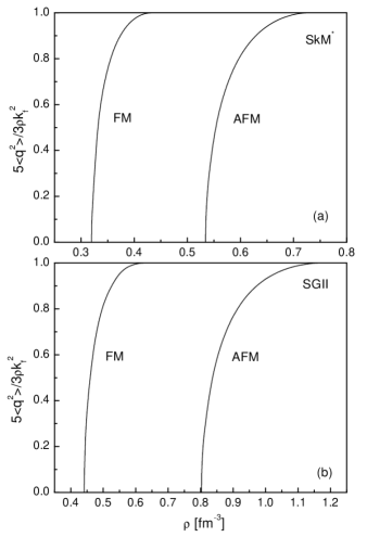
Figure 2: Same as in Fig. 1, but for the second order moments of the distribution functions.

The behavior of these quantities is similar to that of the spin polarization parameters in Fig. 1, with the same values of the threshold densities for the appearance and saturation of the order parameters.

In the density domain, where FM and AFM solutions of self–consistent equations exist simultaneously, it is necessary to clarify, which solution is thermodynamically preferable. To this end, we should compare the free energies of both states. The results of the numerical calculation of the total energy per nucleon, measured from its value in the normal state, are shown in Fig. 3.

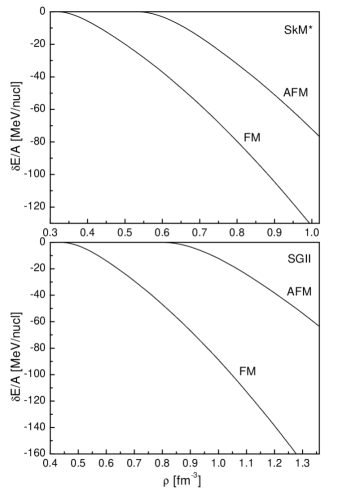
Figure 3: Total energy per nucleon, measured from its value in the normal state, for FM and AFM spin ordering as a function of density at zero temperature for (a) SkM^∗ force and (b) SGII force.

One can see, that for all relevant densities FM spin ordering is more preferable than AFM one, and, moreover, the difference between corresponding free energies becomes larger with increasing density, so that there is no evidence, that AFM spin ordering could become preferable at larger densities. These results are in correspondence with the results of the Brueckner calculations with Nijmegen NSC97e potential in Ref. VB , where it was shown that for symmetric nuclear matter the state with the oppositely directed spins of protons and neutrons is less favorable than the state with the same direction of nucleon spins for all relevant densities. However, in contrast to calculations in Ref. VB , we find that for high density region there will be realized the FM spin ordering of nucleon spins as a ground state of symmetric nuclear matter instead of the nonpolarized state.

IV Phase transitions in strongly asymmetric nuclear matter

In this section we continue to study the properties of spin polarized nuclear matter, but now in the region of large isospin asymmetry. In contrast to symmetric nuclear matter, the analysis shows that in strongly asymmetric nuclear matter it is realized the antiparallel spin ordering of neutron and proton spins.

If all neutron and proton spins are aligned in one direction, then for nontrivial solutions of the self–consistent equations we have

$$\Delta\varrho_{\uparrow\uparrow} =\varrho,\quad\Delta\varrho_{\uparrow\downarrow}=\alpha\varrho,$$ (36)

$$\langle{\bf q}^{2}\rangle_{30} =\frac{3}{10}\varrho k_{F}^{2}[(1+\alpha)^{5/3}+(1-\alpha)^{5/3}],$$

$$\langle{\bf q}^{2}\rangle_{33} =\frac{3}{10}\varrho k_{F}^{2}[(1+\alpha)^{5/3}-(1-\alpha)^{5/3}],$$

where $k_{F}=(3\pi^{2}\varrho)^{1/3}$ is the Fermi momentum of totally polarized symmetric nuclear matter. Therefore, for the partial number densities of nucleons with spin up and spin down one can get

$$\varrho_{n\uparrow}=\frac{1+\alpha}{2}\varrho,\;\varrho_{p\uparrow}=\frac{1-\alpha}{2}\varrho,\;\varrho_{p\downarrow}=\varrho_{n\downarrow}=0.$$ (37)

If all neutron spins are aligned in one direction and all proton spins in the opposite one, then

$$\Delta\varrho_{\uparrow\uparrow} =\alpha\varrho,\quad\Delta\varrho_{\uparrow\downarrow}=\varrho,$$ (38)

$$\langle{\bf q}^{2}\rangle_{30} =\frac{3}{10}\varrho k_{F}^{2}[(1+\alpha)^{5/3}-(1-\alpha)^{5/3}],$$

$$\langle{\bf q}^{2}\rangle_{33} =\frac{3}{10}\varrho k_{F}^{2}[(1+\alpha)^{5/3}+(1-\alpha)^{5/3}],$$

and, hence,

$$\varrho_{n\uparrow}=\frac{1+\alpha}{2}\varrho,\;\varrho_{p\downarrow}=\frac{1-\alpha}{2}\varrho,\;\varrho_{p\uparrow}=\varrho_{n\downarrow}=0.$$ (39)

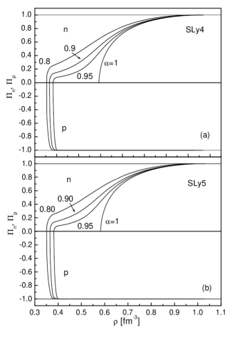
Figure 4: Neutron and proton spin polarization parameters as functions of density at zero temperature for (a) SLy4 force and (b) SLy5 force.

Now we present the results of the numerical solution of the self–consistent equations with the effective SLy4 and SLy5 forces for strongly asymmetric nuclear ($\alpha=0.95,0.9,0.8$) and neutron ($\alpha=1$) matter. The neutron and proton spin polarization parameters $\Pi_{n}$ and $\Pi_{p}$ are shown in Fig. 4 as functions of density at zero temperature. Since in a polarized state the signs of spin polarizations are opposite, considering solutions correspond to the case, when spins of neutrons and protons are aligned in the opposite direction. Note that for SLy4 and SLy5 forces, being relevant for the description of strongly asymmetric nuclear matter, there are no solutions corresponding to the same direction of neutron and proton spins. The reason is that the sign of the multiplier $t_{3}(-1+2x_{3})$ in the density dependent term of the FL amplitude $U_{1}$, determining spin–spin correlations, is positive, and, hence, corresponding term increases with the increase of nuclear matter density, preventing instability with respect to spin fluctuations. Contrarily, the density dependent term $-t_{3}\varrho^{\beta}/3$ in the FL amplitude $U_{3}$, describing spin–isospin correlations, is negative, leading to spin instability with the oppositely directed spins of neutrons and protons at higher densities.

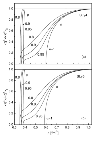
Figure 5: Same as in Fig. 4, but for the second order moments $\langle{\bf q}^{2}\rangle_{p}$ and $\langle{\bf q}^{2}\rangle_{n}$, normalized to their values in the totally polarized state.

Another nontrivial feature relates to the density behavior of the spin polarization parameters at large isospin asymmetry. As seen from Fig. 4, even small admixture of protons leads to the appearance of long tails in the density profiles of the neutron spin polarization parameter near the transition point to a spin ordered state. As a consequence, the spin polarized state is formed much earlier in density than in pure neutron matter. For example, the critical density in neutron matter is $\varrho\approx 0.59\,\mbox{fm}^{-3}$ for SLy4 potential and $\varrho\approx 0.58\,\mbox{fm}^{-3}$ for SLy5 potential; in asymmetric nuclear matter with $\alpha=0.95$ the spin polarized state arises at $\varrho\approx 0.38\,\mbox{fm}^{-3}$ for SLy4 and SLy5 potentials. Hence, even small quantity of protons strongly favors spin instability of highly asymmetric nuclear matter, leading to the appearance of states with the oppositely directed spins of neutrons and protons. As follows from Fig. 4, protons become totally spin polarized within a very narrow density domain (e.g., if $\alpha=0.95$, full polarization occurs at $\varrho\approx 0.41\,\mbox{fm}^{-3}$ for SLy4 force and at $\varrho\approx 0.40\,\mbox{fm}^{-3}$ for SLy5 force) while the threshold densities for the appearance and saturation of the neutron spin order parameter are substantially different (if $\alpha=0.95$, neutrons become totally polarized at $\varrho\approx 1.05\,\mbox{fm}^{-3}$ for SLy4 force and at $\varrho\approx 1.02\,\mbox{fm}^{-3}$ for SLy5 force).

Note that the second order moments

$$\langle{\bf q}^{2}\rangle_{n} \equiv\langle{\bf q}^{2}\rangle_{n\uparrow}-\langle{\bf q}^{2}\rangle_{n\downarrow}$$ (40)

$$=\frac{1}{V}\sum_{\bf q}{\bf q}^{2}\Bigl{(}n(\omega_{+,+})-n(\omega_{-,+})\Bigr{)},$$

$$\langle{\bf q}^{2}\rangle_{p} \equiv\langle{\bf q}^{2}\rangle_{p\uparrow}-\langle{\bf q}^{2}\rangle_{p\downarrow}$$

$$=\frac{1}{V}\sum_{\bf q}{\bf q}^{2}\Bigl{(}n(\omega_{+,-})-n(\omega_{-,-})\Bigr{)}$$

also characterize spin polarization of the neutron and proton subsystems. If the solutions $\langle{\bf q}^{2}\rangle_{30}$ and $\langle{\bf q}^{2}\rangle_{33}$ of the self–consistent equations are known, then

$$\langle{\bf q}^{2}\rangle_{n} =\frac{1}{2}\bigl{(}\langle{\bf q}^{2}\rangle_{30}+\langle{\bf q}^{2}\rangle_{33}\bigr{)},$$

$$\langle{\bf q}^{2}\rangle_{p} =\frac{1}{2}\bigl{(}\langle{\bf q}^{2}\rangle_{30}-\langle{\bf q}^{2}\rangle_{33}\bigr{)}.$$

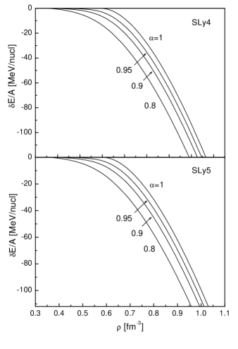
Figure 6: Total energy per nucleon, measured from its value in the normal state, for the state with the oppositely directed spins of neutrons and protons as a function of density at zero temperature for (a) SLy4 force and (b) SLy5 force.

The values of $\langle{\bf q}^{2}\rangle_{n}$ and $\langle{\bf q}^{2}\rangle_{p}$ for the totally polarized state are

$$\langle{\bf q}^{2}\rangle_{n0}=\frac{3}{10}\varrho k_{F}^{2}(1+\alpha)^{5/3},\;\langle{\bf q}^{2}\rangle_{p0}=-\frac{3}{10}\varrho k_{F}^{2}(1-\alpha)^{5/3}.$$

In Fig. 5 we plot the density dependence of the second order moments $\langle{\bf q}^{2}\rangle_{n}$ and $\langle{\bf q}^{2}\rangle_{p}$, normalized to their values in the totally polarized state, for different asymmetries at zero temperature. These quantities behave similarly to the spin polarization parameters in Fig. 4, i.e., there exist long tails in the density profiles of the neutron spin order parameter and the proton spin order parameter is saturated within a very narrow density interval.

To check thermodynamic stability of the spin ordered state with the oppositely directed spins of neutrons and protons, it is necessary to compare the free energies of this state and the normal state. In Fig. 6 the difference between the total energies per nucleon of the spin ordered and normal states is shown as a function of density at zero temperature. One can see that nuclear matter undergoes a phase transition to the state with the oppositely directed spins of neutrons and protons at some critical density, depending on the isospin asymmetry.

Note that our results of neutron matter calculations obtained with the Skyrme effective interaction predict a FM phase transition at some critical density, that is different from the results of calculations with realistic NN potentials VPR ; FSS . In Ref. VPR , employing Nijmegen II and Reid93 NN potentials, it has been found within the Brueckner–Hartree–Fock approach, that in the range of densities explored ($\varrho\lesssim 7\varrho_{0}$) totally polarized neutron matter is always more repulsive than nonpolarized matter, being an indication that a phase transition of neutron matter to a FM state is not expected. Besides, in Ref. FSS , in connection with the problem of the neutrino diffusion in dense matter, it has been shown within the framework of the auxiliary field diffusion Monte Carlo method with the Argonne $v_{18}$ two–body potential and Urbana IX three–body potential, that the magnetic susceptibility of neutron matter shows a strong reduction of about a factor 3 with respect to its Fermi gas value. However, calculations of the magnetic susceptibility with the Skyrme effective interaction VNB give indication of infinite discontinuity, and, hence, predict a FM transition at densities $\varrho\approx 0.18-0.26\,\mbox{fm}^{-3}$.

For strongly asymmetric nuclear matter with Skyrme forces we find a phase transition to the state with antiparallel spins of neutrons and protons, that is different from the results of calculations with NSC97e NN potential in Ref. VB , where the nonpolarized state was predicted for the whole range of densities up to 1.2 $\mbox{fm}^{-3}$. The reasons, explaining such disagreement in calculations with the effective and realistic NN potentials, are discussed in the next section.

V Discussion and Conclusions

Spin instability is a common feature, associated with a large class of Skyrme models, but is not realized in more microscopic calculations. The Skyrme interaction has been successful in describing nuclei and their excited states. In addition, various authors have exploited its applicability to describe bulk matter at densities of relevance to neutron stars SMK . The force parameters are determined empirically by calculating the ground state in the Hartree–Fock approximation and by fitting the observed ground state properties of nuclei and nuclear matter at the saturation density. In particular, the interaction parameters, describing spin–spin and spin–isospin correlations, are constrained from the data on isoscalar T ; LS and isovector (giant Gamow–Teller) HHR ; SGE ; BDE spin–flip resonances.

In a microscopic approach, one starts with the bare interaction and obtains an effective particle–hole interaction by solving iteratively the Bethe–Goldstone equation. In contrast to the Skyrme models, calculations with realistic NN potentials predict more repulsive total energy per particle for a polarized state comparing to the nonpolarized one for all relevant densities, and, hence, give no indication of a phase transition to a spin ordered state. It must be emphasized that the interaction in the spin– and isospin–dependent channels is a crucial ingredient in calculating spin properties of isospin symmetric and asymmetric nuclear matter and different behavior at high densities of the interaction amplitudes, describing spin–spin and spin–isospin correlations, lays behind this divergence in calculations with the effective and realistic potentials.

In this study as a potential of NN interaction we chose SkM^∗ and SGII (symmetric nuclear matter) as well as SLy4 and SLy5 (strongly asymmetric nuclear matter) Skyrme effective forces. The models SkM^∗ and SGII SG have been constrained by fitting the properties of nucleon systems with very small isospin asymmetries, while the models SLy4 and SLy5 were further constrained to reproduce the results of microscopic neutron matter calculations (pressure versus density curve) CBH . Besides, in a recent publication SMK it was shown that the density dependence of the nuclear symmetry energy, calculated up to densities $\varrho\lesssim 3\varrho_{0}$ with SLy4 and SLy5 effective forces (together with some other sets of parameters among the total 87 Skyrme force parametrizations checked) gives the neutron star models in a broad agreement with the observables, such as the minimum rotation period, gravitational mass–radius relation, the binding energy, released in supernova collapse, etc. This is an important check for using these parametrizations in the high density region of strongly asymmetric nuclear matter. However, it is necessary to note, that the spin–dependent part of the Skyrme interaction at densities of relevance to neutron stars still remains to be constrained. Probably, these constraints will be obtained from the data on the time decay of magnetic field of isolated neutron stars PP . In spite of this shortcoming, SLy4 and SLy5 effective forces hold one of the most competing Skyrme parametrizations at present time for description of isospin asymmetric nuclear matter at high density (together with SkM^∗ and SGII forces for description of symmetric nuclear matter) while a Fermi liquid approach with Skyrme effective forces provides a consistent and transparent framework for studying spin instabilities in a nucleon system.

In summary, we have considered the possibility of phase transitions into spin ordered states of symmetric and strongly asymmetric nuclear matter within the Fermi liquid formalism, where NN interaction is described by the Skyrme effective forces (SkM^∗, SGII and SLy4, SLy5 potentials for the regions of vanishing and strong isospin asymmetry, respectively). In contrast to the previous considerations, where the possibility of formation of FM spin polarized states was studied on the base of calculation of magnetic susceptibility, we obtain the self–consistent equations for the FM and AFM spin order parameters and solve them in the case of zero temperature. It has been found that nuclear matter demonstrates different behavior at high densities with respect to spin fluctuations in isospin symmetric and strongly isospin asymmetric cases. In the model with SkM^∗ and SGII effective forces symmetric nuclear matter undergoes a FM phase transition, when the spins of protons and neutrons are aligned along the same direction. In the model with SLy4 and SLy5 effective forces strongly asymmetric nuclear matter is subjected to a phase transition into the spin polarized state with the oppositely directed spins of neutrons and protons, while the state with the same direction of the neutron and proton spins does not appear. In the last case, an important peculiarity of the corresponding phase transition is the existence of long tails in the density profile of the neutron spin polarization parameter near the transition point. This means that even small admixture of protons to neutron matter leads to a considerable shift of the critical density of spin instability in the direction of low densities. In the model with SLy4 effective interaction this displacement is from the critical density $\varrho\approx 3.7\varrho_{0}$ for neutron matter to $\varrho\approx 2.4\varrho_{0}$ for asymmetric nuclear matter at the isospin asymmetry $\alpha=0.95$, i.e. for $2.5\%$ of protons only. As a result, the state with the oppositely directed spins of neutrons and protons appears, where protons become totally polarized in a very narrow density domain.

As a consequence of this study, important questions appear, what is the value of the threshold asymmetry, at which the parallel spin ordering at small isospin asymmetry is changed to the antiparallel spin ordering at large isospin asymmetry, and do the obtained results survive for another type of an effective interaction, e.g., for Gogny effective force BGG ; FVS or monopole effective interaction RSM ? This research is in progress and will be reported elsewhere.

Appendix

The aim of this section is to establish relationships between the Fermi liquid amplitudes and amplitudes of NN interaction in the leading order on the interaction between nucleons. To this end we present the Hamiltonian of the system in the form

$$H =H_{0}+V,$$ (41)

$$H_{0}=\sum_{\kappa_{1}\kappa_{2}}\varepsilon^{0}_{\kappa_{1}\kappa_{2}}a^{+}_{\kappa_{1}}a_{\kappa_{2}},\quad V =\frac{1}{2\cal V}\sum_{\kappa_{1}\kappa_{2}\kappa_{3}\kappa_{4}}\hat{v}(\kappa_{1}\kappa_{2};\kappa_{3}\kappa_{4})a^{+}_{\kappa_{1}}a^{+}_{\kappa_{2}}a_{\kappa_{4}}a_{\kappa_{3}},$$

where $\hat{v}$ is the amplitude of NN interaction. We shall assume that the amplitude $\hat{v}$ doesn’t depend on the total momentum of colliding nucleons, but only from their relative momenta:

$$\hat{v}(\kappa_{1}\kappa_{2};\kappa_{3}\kappa_{4}) =\hat{v}({\bf p}_{1},{\bf p}_{2};{\bf p}_{3},{\bf p}_{4})_{\underline{\kappa}_{1}\underline{\kappa}_{2};\underline{\kappa}_{3}\underline{\kappa}_{4}},\quad\underline{\kappa}\equiv(\sigma,\tau),$$ (42)

$$\hat{v}({\bf p}_{1},{\bf p}_{2};{\bf p}_{3},{\bf p}_{4})_{\underline{\kappa}_{1}\underline{\kappa}_{2};\underline{\kappa}_{3}\underline{\kappa}_{4}} =\hat{v}({\bf p},{\bf q})_{\underline{\kappa}_{1}\underline{\kappa}_{2};\underline{\kappa}_{3}\underline{\kappa}_{4}};\quad{\bf p}=\frac{{\bf p}_{1}-{\bf p}_{2}}{2},\;{\bf q}=\frac{{\bf p}_{3}-{\bf p}_{4}}{2}.$$

To obtain the energy functional, corresponding to the Hamiltonian (41), we should average the Hamiltonian (41) over the state of nonideal gas of particles. In the leading approximation on the interaction, using the Wick rules and taking into account that $\mbox{Tr}\varrho a^{+}_{\kappa_{2}}a_{\kappa_{1}}\equiv f_{\kappa_{1}\kappa_{2}}$ ($\varrho$ being the statistical operator), one gets

$$E(f) =E_{0}(f)+E_{int}(f)$$ (43)

$$E_{0}(f)=\sum_{\kappa_{1}\kappa_{2}}\varepsilon^{0}_{\kappa_{1}\kappa_{2}}f_{\kappa_{2}\kappa_{1}},\quad E_{int}(f) =\frac{1}{2\cal V}\sum_{\kappa_{1}\kappa_{2}\kappa_{3}\kappa_{4}}\hat{v}(\kappa_{1}\kappa_{2};\kappa_{3}\kappa_{4})\bigl{(}f_{\kappa_{3}\kappa_{1}}f_{\kappa_{4}\kappa_{2}}-f_{\kappa_{4}\kappa_{1}}f_{\kappa_{3}\kappa_{2}}\bigr{)}.$$

Hence, according to Eq. (1), expression for the single particle energy reads

$$\varepsilon_{\kappa_{1}\kappa_{2}} =\varepsilon_{\kappa_{1}\kappa_{2}}^{0}(f)+\tilde{\varepsilon}_{\kappa_{1}\kappa_{2}}(f),$$ (44)

$$\tilde{\varepsilon}_{\kappa_{1}\kappa_{2}}(f)=\frac{1}{2\cal V}\sum_{\kappa_{3}\kappa_{4}}\bigl{\{}\hat{v}(\kappa_{1}\kappa_{3};\kappa_{2}\kappa_{4}) +\hat{v}(\kappa_{3}\kappa_{1};\kappa_{4}\kappa_{2})-\hat{v}(\kappa_{1}\kappa_{3};\kappa_{4}\kappa_{2})-\hat{v}(\kappa_{3}\kappa_{1};\kappa_{2}\kappa_{4})\bigr{\}}f_{\kappa_{4}\kappa_{3}}.$$

For spatially homogeneous distributions

$$f_{\kappa_{1}\kappa_{2}}=f_{\underline{\kappa}_{1}\underline{\kappa}_{2}}({\bf p}_{1})\delta_{p_{1},p_{2}},\quad\varepsilon_{\kappa_{1}\kappa_{2}}=\varepsilon_{\underline{\kappa}_{1}\underline{\kappa}_{2}}({\bf p_{1}})\delta_{p_{1},p_{2}}$$ (45)

and Eqs. (43), (44) can be simplified

$$E_{0}(f) =\sum_{\underline{\kappa}_{1},\underline{\kappa}_{2};\,\bf p}\varepsilon^{0}_{\underline{\kappa}_{1}\underline{\kappa}_{2}}({\bf p})f_{\underline{\kappa}_{2}\underline{\kappa}_{1}}({\bf p}),$$ (46)

$$E_{int}(f) =\frac{1}{2}\sum_{\underline{\kappa}_{1},\underline{\kappa}_{2};\,{\bf p}}\tilde{\varepsilon}_{\underline{\kappa}_{1}\underline{\kappa}_{2}}({\bf p})f_{\underline{\kappa}_{2}\underline{\kappa}_{1}}({\bf p}),$$

where

$$\tilde{\varepsilon}_{\underline{\kappa}_{1}\underline{\kappa}_{2}}({\bf p}) =\frac{1}{2\cal V}\sum_{\underline{\kappa}_{3}\underline{\kappa}_{4}}\bigl{\{}\hat{v}_{\underline{\kappa}_{1}\underline{\kappa}_{3};\underline{\kappa}_{2}\underline{\kappa}_{4}}({\bf k},{\bf k})+\hat{v}_{\underline{\kappa}_{3}\underline{\kappa}_{1};\underline{\kappa}_{4}\underline{\kappa}_{2}}(-{\bf k},-{\bf k})$$ (47)

$$\quad-\hat{v}_{\underline{\kappa}_{1}\underline{\kappa}_{3};\underline{\kappa}_{4}\underline{\kappa}_{2}}({\bf k},-{\bf k})-\hat{v}_{\underline{\kappa}_{3}\underline{\kappa}_{1};\underline{\kappa}_{2}\underline{\kappa}_{4}}(-{\bf k},{\bf k})\bigr{\}}f_{\underline{\kappa}_{4}\underline{\kappa}_{3}}({\bf q}),\quad{\bf k}=\frac{{\bf p}-{\bf q}}{2}.$$

The general structure of the NN interaction amplitude $\hat{v}$, invariant with respect to rotations in spin and isospin spaces, has the form

$$\hat{v}({\bf p},{\bf q})=v_{0}({\bf p},{\bf q})+v_{1}({\bf p},{\bf q}){{\boldsymbol{\sigma}_{1}\boldsymbol{\sigma}_{2}}}+v_{2}({\bf p},{\bf q}){{\boldsymbol{\tau}_{1}\boldsymbol{\tau}_{2}}}+v_{3}({\bf p},{\bf q})({{\boldsymbol{\sigma}_{1}\boldsymbol{\sigma}_{2}}})({{\boldsymbol{\tau}_{1}\boldsymbol{\tau}_{2}}}).$$ (48)

Taking into account the general structure of the normal distribution function

$$f({\bf p})=f_{00}({\bf p})+f_{k0}({\bf p})\sigma_{k}+f_{0l}({\bf p})\tau_{l}+f_{kl}({\bf p})\sigma_{k}\tau_{l}$$ (49)

and calculating traces in Eqs. (46), (47), one can get

$${E}_{0}(f) =4\sum\limits_{\bf p}\varepsilon_{0}({\bf p})f_{00}({\bf p}),\;\varepsilon_{0}({\bf p})=\frac{{\bf p}^{\,2}}{2m_{0}},$$ (50)

$${E}_{int}(f) =2\sum\limits_{\bf p}\{\tilde{\varepsilon}_{00}({\bf p})f_{00}({\bf p})+\tilde{\varepsilon}_{k0}({\bf p})f_{k0}({\bf p})$$ (51)

$$\quad+\tilde{\varepsilon}_{0l}({\bf p})f_{0l}({\bf p})+\tilde{\varepsilon}_{kl}({\bf p})f_{kl}({\bf p})\},$$

$$\tilde{\varepsilon}_{00}({\bf p}) =\frac{1}{2\cal V}\sum_{\bf q}U_{0}({\bf k})f_{00}({\bf q}),\;{\bf k}=\frac{{\bf p}-{\bf q}}{2},$$

$$\tilde{\varepsilon}_{k0}({\bf p}) =\frac{1}{2\cal V}\sum_{\bf q}U_{1}({\bf k})f_{k0}({\bf q}),$$

$$\tilde{\varepsilon}_{0l}({\bf p}) =\frac{1}{2\cal V}\sum_{\bf q}U_{2}({\bf k})f_{0l}({\bf q}),$$

$$\tilde{\varepsilon}_{kl}({\bf p}) =\frac{1}{2\cal V}\sum_{\bf q}U_{3}({\bf k})f_{kl}({\bf q}),$$

where

$$U_{0}({\bf k}) =\bigl{\{}4v_{0}({\bf k},{\bf k})-v_{0}(-{\bf k},{\bf k})-3v_{1}(-{\bf k},{\bf k})-3v_{2}(-{\bf k},{\bf k})-9v_{3}(-{\bf k},{\bf k})\bigr{\}}+\bigl{\{}{\bf k}\rightarrow-{\bf k}\bigr{\}},$$

$$U_{1}({\bf k}) =\bigl{\{}4v_{1}({\bf k},{\bf k})-v_{0}(-{\bf k},{\bf k})+v_{1}(-{\bf k},{\bf k})-3v_{2}(-{\bf k},{\bf k})+3v_{3}(-{\bf k},{\bf k})\bigr{\}}+\bigl{\{}{\bf k}\rightarrow-{\bf k}\bigr{\}},$$ (52)

$$U_{2}({\bf k}) =\bigl{\{}4v_{2}({\bf k},{\bf k})-v_{0}(-{\bf k},{\bf k})-3v_{1}(-{\bf k},{\bf k})+v_{2}(-{\bf k},{\bf k})+3v_{3}(-{\bf k},{\bf k})\bigr{\}}+\bigl{\{}{\bf k}\rightarrow-{\bf k}\bigr{\}},$$

$$U_{3}({\bf k}) =\bigl{\{}4v_{3}({\bf k},{\bf k})-v_{0}(-{\bf k},{\bf k})+v_{1}(-{\bf k},{\bf k})+v_{2}(-{\bf k},{\bf k})-v_{3}(-{\bf k},{\bf k})\bigr{\}}+\bigl{\{}{\bf k}\rightarrow-{\bf k}\bigr{\}}.$$

The interaction energy functional (13) represents a special case of the functional (51), corresponding to a collinear spin ordering. The amplitude of NN interaction for the Skyrme effective forces has the form

$$\hat{v}({\bf p},{\bf q}) =t_{0}(1+x_{0}P_{\sigma})+\frac{1}{6}t_{3}(1+x_{3}P_{\sigma})\varrho^{\beta}+\frac{1}{2\hbar^{2}}t_{1}(1+x_{1}P_{\sigma})({\bf p}^{2}+{\bf q}^{2})$$ (53)

$$\quad+\frac{t_{2}}{\hbar^{2}}(1+x_{2}P_{\sigma}){\bf p}{\bf q},\quad P_{\sigma}=\frac{1}{2}(1+{{\boldsymbol{\sigma}_{1}\boldsymbol{\sigma}_{2}}}),$$

Here $P_{\sigma}$ is the spin exchange operator. Extracting from Eq. (53) the functions $v_{0},...,v_{3}$ and substituting their expressions into Eq. (52), we obtain Eqs. (15) for the normal FL amplitudes $U_{0},...,U_{3}$, describing, respectively, density, spin, isospin and spin–isospin correlations in a nucleon Fermi liquid.

For neutron matter the basic equations (43), (44) remain unchanged, but now the individual state of a neutron is characterized by momentum $\bf p$ and spin projection $\sigma$, $\kappa\equiv({\bf p},\sigma)$. Besides, taking into account the general structure of the interaction amplitude $\hat{v}$ and the normal distribution function $f$

$$\hat{v}({\bf p},{\bf q}) =v_{0}({\bf p},{\bf q})+v_{1}({\bf p},{\bf q}){{\boldsymbol{\sigma}_{1}\boldsymbol{\sigma}_{2}}},$$ (54)

$$f({\bf p}) =f_{0}({\bf p})+f_{k}({\bf p})\sigma_{k},$$ (55)

and calculating traces with the Pauli matrices $\sigma_{i}$, we obtain

$${E}_{0}(f) =2\sum\limits_{\bf p}\varepsilon_{0}({\bf p})f_{0}({\bf p}),\;\varepsilon_{0}({\bf p})=\frac{{\bf p}^{\,2}}{2m_{0}},$$

$${E}_{int}(f) =\sum\limits_{\bf p}\{\tilde{\varepsilon}_{0}({\bf p})f_{0}({\bf p})+\tilde{\varepsilon}_{k}({\bf p})f_{k}({\bf p})\},$$

where

$$\tilde{\varepsilon}_{0}({\bf p}) =\frac{1}{2\cal V}\sum_{\bf q}U_{0}^{n}({\bf k})f_{0}({\bf q}),\;{\bf k}=\frac{{\bf p}-{\bf q}}{2},$$ (56)

$$\tilde{\varepsilon}_{k}({\bf p}) =\frac{1}{2\cal V}\sum_{\bf q}U_{1}^{n}({\bf k})f_{k}({\bf q}),$$

and the FL amplitudes are given by the formulas

$$U_{0}^{n}({\bf k}) =\bigl{\{}2v_{0}({\bf k},{\bf k})-v_{0}(-{\bf k},{\bf k})-3v_{1}(-{\bf k},{\bf k})\bigr{\}}+\bigl{\{}{\bf k}\rightarrow-{\bf k}\bigr{\}},$$ (57)

$$U_{1}^{n}({\bf k}) =\bigl{\{}2v_{1}({\bf k},{\bf k})-v_{0}(-{\bf k},{\bf k})+v_{1}(-{\bf k},{\bf k})\bigr{\}}+\bigl{\{}{\bf k}\rightarrow-{\bf k}\bigr{\}}.$$

After substituting expressions for the functions $v_{0},v_{1}$ from Eq. (53), we obtain Eqs. (24), (25) for the neutron matter FL amplitudes $U_{0}^{n},U_{1}^{n}$.

References

• (1) M.J. Rice, Phys. Lett. 29A, 637 (1969).
• (2) S.D. Silverstein, Phys. Rev. Lett. 23, 139 (1969).
• (3) E. Østgaard, Nucl. Phys. A154, 202 (1970).
• (4) A. Viduarre, J. Navarro, and J. Bernabeu, Astron. Astrophys. 135, 361 (1984).
• (5) S. Reddy, M. Prakash, J.M. Lattimer, and J.A. Pons, Phys. Rev. C 59, 2888 (1999).
• (6) A.I. Akhiezer, N.V. Laskin, and S.V. Peletminsky, Phys. Lett. 383B, 444 (1996); Sov. Phys. JETP 82, 1066 (1996).
• (7) S. Marcos, R. Niembro, M.L. Quelle, and J. Navarro, Phys. Lett. 271B, 277 (1991).
• (8) T. Maruyama and T. Tatsumi, Nucl. Phys. A693, 710 (2001).
• (9) M. Kutschera, and W. Wojcik, Phys. Lett. 223B, 11 (1989).
• (10) P. Bernardos, S. Marcos, R. Niembro, and M.L. Quelle, Phys. Lett. 356B, 175 (1995).
• (11) V.R. Pandharipande, V.K. Garde, and J.K. Srivastava, Phys. Lett. 38B, 485 (1972).
• (12) S.O. Bäckmann and C.G. Källman, Phys. Lett. 43B, 263 (1973).
• (13) P. Haensel,Phys. Rev. C 11, 1822 (1975).
• (14) I. Vida$\tilde{\mbox{n}}$a, A. Polls, and A. Ramos, Phys. Rev. C 65, 035804 (2002).
• (15) I. Vida$\tilde{\mbox{n}}$a, and I. Bombaci, Phys. Rev. C 66, 045801 (2002).
• (16) S. Fantoni, A. Sarsa, and E. Schmidt, Phys. Rev. Lett. 87, 181101 (2001).
• (17) A.I. Akhiezer, V.V. Krasil’nikov, S.V. Peletminsky, and A.A. Yatsenko, Phys. Rep. 245, 1 (1994).
• (18) A.I. Akhiezer, A.A. Isayev, S.V. Peletminsky, A.P. Rekalo, and A.A. Yatsenko, Sov. Phys. JETP 85, 1 (1997).
• (19) R.K. Su, S.D. Yang, and T.T.S. Kuo, Phys. Rev. C 35, 1539 (1987).
• (20) M.F. Jiang and T.T.S. Kuo, Nucl. Phys. A481, 294 (1988).
• (21) A.I. Akhiezer, A.A. Isayev, S.V. Peletminsky, and A.A. Yatsenko, Phys. Rev. C 63, 021304(R) (2001).
• (22) A.A. Isayev, Phys. Rev. C 65, 031302(R) (2002).
• (23) A.A. Isayev, JETP Letters 77, 251 (2003).
• (24) A.A. Isayev, J. Yang, Phys. Rev. C 69, 025801 (2004).
• (25) P. Haensel, and A.J. Jerzak, Phys. Lett. 112B, 285 (1982).
• (26) J. Dobrowski, Can. J. Phys. 62, 400 (1984).
• (27) T. Frick, H. Müther, and A. Sedrakian, Phys. Rev. C 65, 061303(R) (2002).
• (28) M. Brack, C. Guet and H.-B. Hakansson, Phys. Rep. 123, 275 (1985).
• (29) N. V. Giai, and H. Sagawa, Phys. Lett. 106B, 379 (1981).
• (30) E. Chabanat, P. Bonche, P. Haensel, J. Meyer, and R. Schaeffer, Nucl. Phys. A635, 231 (1998).
• (31) J. Rikovska Stone, J.C. Miller, R. Koncewicz, P.D. Stevenson, and M.R. Strayer, Phys. Rev. C 68, 034324 (2003).
• (32) I.S. Towner, Phys. Rep. 155, 263 (1987).
• (33) W.G. Love and J. Speth, Comments Nucl. Part. Phys. 14, 185 (1985).
• (34) R.R. Hilton, W. Höhenberger and P. Ring, Eur. Phys. J. A 1, 257 (1998).
• (35) P. Sarriguren, E.M. de Guerra, and A. Escuderos, Nucl. Phys. A658, 13 (1999); A691, 631 (2001).
• (36) M. Bender, J. Dobaczewski, J. Engel, and W. Nazarewicz, Phys. Rev. C 65, 054322 (2002).
• (37) S.B. Popov and M.E. Prokhorov, Surv. in High Energy Phys. 15, 381 (2001).
• (38) J.F. Berger, M. Girod and D. Gogny, Comp. Phys. Comm. 63, 365 (1991).
• (39) M. Farine, D. Von–Eiff, P. Schuck, J.F. Berger, J. Decharge, and M. Girod, J. Phys. G 25, 863 (1999).
• (40) J. Rikovska Stone, P.D. Stevenson, J.C. Miller, and M.R. Strayer, Phys. Rev. C 65, 064312 (2002).