An Introduction to Nuclear Supersymmetry: a Unification Scheme for Nuclei

Abstract

The main ideas behind nuclear supersymmetry are presented, starting from the basic concepts of symmetry and the methods of group theory in physics. We propose new, more stringent experimental tests that probe the supersymmetry classification in nuclei and point out that specific correlations should exist for particle transfer intensities among supersymmetric partners. We also discuss possible ways to generalize these ideas to cases where no dynamical symmetries are present. The combination of these theoretical and experimental studies may play a unifying role in nuclear phenomena.

1 Introduction

One of the main objectives of research in physics is to find simple laws that give rise to a deeper understanding and/or a unification of diverse phenomena. A less ambitious goal is to construct models which, in a more or less restricted range, permit an understanding of the physical processes involved and give rise to a systematic analysis of the available experimental data, while providing insights into the complex systems being studied. Among models of nuclear structure,the Interacting Boson Model and its extensions have proved remarkably successful in providing a unified framework for even-even IBM and odd-A nuclei IBFM . One of its most attractive features is that it gives rise to a simple algebraic description, where the so-called dynamical symmetries play a central role, both as a way to improve our basic understanding of the role of symmetry in nuclear dynamics and as starting points from which more precise calculations can be carried out. This approach has, in a first stage, produced a unified description of the properties of medium and heavy even-even nuclei, which are pictured in this framework as belonging (in general) to transitional regions between the dynamical symmetries. Later on, odd-A nuclei were also analyzed using this point of view IBFM . A further step was then taken by Iachello FI , who suggested that a simultaneous description of even-even and odd-A nuclei was possible through the introduction of a superalgebra, energy levels in both nuclei belonging to the same (super)multiplet. The idea was subsequently tested in several regions of the nuclear table susy ; baha ; mauthofer1 ; thesis ; siete . The step of including the odd-odd nucleus into this unifying framework was then taken by Van Isacker et al quartet , who managed to formulate a supersymmetric theory for quartets of nuclei.

In the artistic interpretation of Fig. 1 by Renato Lemus, supersymmetric quartets of nuclei are described using the language of old Nahua Codices (compare with Eq. (126) in Section 3.4). Four aztec gods play the role of the supersymmetric nuclei in a quartet. The gods are depicted as players of the “Juego de Pelota”, the ritual game of prehispanic cultures. The players carry 7 balls each which are color-coded. Green and blue balls correspond to neutron and proton bosons, while yellow and red ones to neutron and protons, respectively. Transfer operators are represented by coral snakes (“coralillo”), the traditional symbol of transformation. Creation and annihilation operators are identified by balls carried by the snakes, transforming one “God” into another. A more detailed explanation can be obtained from the artist at renato@nuclecu.unam.mx.

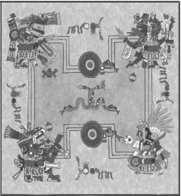
Figure 1: Precolumbian Supersymmetry

In these lecture notes we describe the basic theoretical ideas underlying nuclear symmetry and supersymmetry (SUSY). We start these lecture notes by giving a description of the mathematical framework needed for the understanding of symmetries in nature, which is that of group theory and Lie Algebras. In the subsequent sections we then concentrate on theoretical and experimental aspects of nuclear supersymmetry. A pedagogic description of algebraic techniques in nuclei and molecules can be found in nueve , from which some of the following discussions have been taken.

2 Symmetries and Group Theory

Symmetry and its mathematical framework—group theory—play an increasingly important role in physics. Both classical and quantum systems usually display great complexity, but the analysis of their symmetry properties often gives rise to simplifications and new insights which can lead to a deeper understanding. In addition, symmetries themselves can point the way toward the formulation of a correct physical theory by providing constraints and guidelines in an otherwise intractable situation. It is remarkable that, in spite of the wide variety of systems one may consider, all the way from classical ones to molecules, nuclei, and elementary particles, group theory applies the same basic principles and extracts the same kind of useful information from all of them. This universality in the applicability of symmetry considerations is one of the most attractive features of group theory. Most people have an intuitive understanding of symmetry, particularly in its most obvious manifestation in terms of geometric transformations that leave a body or system invariant. This interpretation, however, is not enough to readily grasp its deep connections with physics, and it thus becomes necessary to generalize the notion of symmetry transformations to encompass more abstract ideas. The mathematical theory of these transformations is the subject matter of group theory. When these operations are of a continuous nature, one can always consider the case of infinitesimal transformations and study the behavior of the systems subject to the latter. The mathematical theory of such transformations was first considered by Marius Sophus Lie, who introduced the basic concepts and operations of what are now called Lie algebras aGIL74 .

2.1 Some Definitions

An abstract group $G$ is defined by a set of elements $(\hat{G}_{1},\hat{G}_{2},\dots,\hat{G}_{n})$ for which a “multiplication” rule combining these elements exists and which satisfies the following conditions:

1. Closure:
   If $\hat{G}_{i}$ and $\hat{G}_{j}$ are elements of the set, so is their product $\hat{G}_{i}\hat{G}_{j}$.

2. Associativity:
   The following property is always valid:

   $$\hat{G}_{i}(\hat{G}_{j}\hat{G}_{k})=(\hat{G}_{i}\hat{G}_{j})\hat{G}_{k}~{}.$$

3. Identity:
   There exists an element $\hat{E}$ of $G$ satisfying

   $$\hat{E}\hat{G}_{i}=\hat{G}_{i}\hat{E}=\hat{G}_{i}~{}.$$

4. Inverse:
   For every $\hat{G}_{i}$ there exists an element $\hat{G}_{i}^{-1}$ such that

   $$\hat{G}_{i}\hat{G}_{i}^{-1}=\hat{G}_{i}^{-1}\hat{G}_{i}=\hat{E}~{}.$$

The number $n$ of elements is called the order of the group. For continuous (or Lie) groups all elements may be obtained by exponentiation in terms of a basic set of elements $\hat{g}_{i},i=1,2,\dots,s$, called generators, which together form the Lie algebra associated with the Lie group. A simple example is provided by the SO(2) group of rotations in two-dimensional space, with elements that may be realized as

$$\hat{G}(\alpha)=e^{-i\alpha\hat{l}_{z}}~{},$$ (1)

where $\alpha$ is the angle of rotation and

$$\hat{l}_{z}=-i\left(x{\frac{\partial}{\partial y}}-y{\frac{\partial}{\partial x}}\right)~{},$$ (2)

is the generator of these transformations in the $x$–$y$ plane. Three-dimensional rotations require the introduction of two additional generators, associated with rotations in the $z$–$x$ and $y$–$z$ planes,

$$\hat{l}_{y}=-i\left(z{\frac{\partial}{\partial x}}-x{\frac{\partial}{\partial z}}\right)~{},\qquad\hat{l}_{x}=-i\left(y{\frac{\partial}{\partial z}}-z{\frac{\partial}{\partial y}}\right)~{},$$ (3)

Finite rotations can then be parametrized by three angles (which may be chosen to be the Euler angles) and expressed as a product of exponentials of the so(3) generators (2) and (3) aROS57 . Evaluating the commutators of these operators, we find

$$[\hat{l}_{x},\hat{l}_{y}]=i\hat{l}_{z}~{},\qquad[\hat{l}_{y},\hat{l}_{z}]=i\hat{l}_{x}~{},\qquad[\hat{l}_{z},\hat{l}_{x}]=i\hat{l}_{y}~{},$$ (4)

which illustrates the closure property of the group generators. In general, the $s$ operators $\hat{g}_{i},i=1,2,\dots,s$, define a Lie algebra if they close under commutation,

$$[\hat{g}_{i},\hat{g}_{j}]=\sum_{k}c^{k}_{ij}\hat{g}_{k}~{},$$ (5)

and satisfy the Jacobi identity aWYB74

$$[\hat{g}_{i},[\hat{g}_{j},\hat{g}_{k}]]+[\hat{g}_{k},[\hat{g}_{i},\hat{g}_{j}]]+[\hat{g}_{j},[\hat{g}_{k},\hat{g}_{i}]]=0~{}.$$ (6)

The set of constants $c^{k}_{ij}$ are called structure constants, and their values determine the properties of both the Lie algebra and its associated Lie group. All Lie groups have been classified by Cartan aWYB74 ; aLIP66 , and many of their properties have been established.

2.2 Symmetry Transformations

From a general point of view symmetry transformations of a physical system may be defined in terms of the equations of motion for the system aMAN91 . Suppose we consider the system of equations

$${\cal O}_{i}\psi_{i}({\bf x})=0~{},\qquad i=1,2,\dots~{},$$ (7)

where the functions $\psi_{i}({\bf x})$ denote a vector column with a finite or infinite number of components, or a more general structure such as a matrix depending on the variables $x_{i}$. The operators $\cal{O}_{i}$ are quite arbitrary, and (7) may correspond, for example, to Maxwell, Schrödinger, or Dirac equations. The operators $\hat{g}_{ij}$ such that

$$\sum_{j}{\cal O}_{i}(\hat{g}_{ij}\psi_{j})=0,\qquad i=1,2,\dots~{},$$ (8)

are called symmetry transformations, since they transform the solutions $\psi$ to other solutions $g\psi$ of the equations (7). As a particular example we consider the time-dependent Schrödinger equation (with $\hbar=1$)

$$\left(\hat{H}({\bf x},{\bf p})-i\frac{\partial}{\partial t}\right)\psi({\bf x},t)=0~{}.$$ (9)

One can verify that $\hat{k}_{j}({\bf x},{\bf p},t)\psi({\bf x},t)$ is also a solution of (9) as long as $\hat{k}_{j}$ satisfies the equation

$$[\hat{H},\hat{k}_{j}]-i{{\partial\hat{k}_{j}}\over{\partial t}}=0~{},$$ (10)

which means that $\hat{k}_{j}$ is an operator associated with a conserved quantity. The last statement follows from the definition of the total derivative of an operator $\hat{A}_{j}$

$${{d\hat{A}_{j}}\over{dt}}={{\partial\hat{A}_{j}}\over{\partial t}}+i[\hat{H},\hat{A}_{j}]~{},$$ (11)

where $\hat{H}$ is the quantum-mechanical Hamiltonian aMES68 . If $\hat{k}_{1}$ and $\hat{k}_{2}$ satisfy (10), their commutator is again a constant of the motion since

$$\frac{d}{dt}[\hat{k}_{1},\hat{k}_{2}] = \frac{\partial}{\partial t}[\hat{k}_{1},\hat{k}_{2}]+i[\hat{H},[\hat{k}_{1},\hat{k}_{2}]]$$ (12)

$$= \frac{\partial}{\partial t}[\hat{k}_{1},\hat{k}_{2}]-[{{\partial\hat{k}_{1}}\over{\partial t}},\hat{k}_{2}]-[\hat{k}_{1},{{\partial\hat{k}_{2}}\over{\partial t}}]=0~{},$$

where use is made of (10) and the Jacobi identity (6). A particularly interesting situation arises when the set $(\hat{k}_{i})$ is such that $[\hat{k}_{i},\hat{k}_{j}]$ closes under commutation to form a Lie algebra as in (5). In this case we refer to $(\hat{k}_{i})$ as the generators of the symmetry (Lie) algebra of the time-dependent quantum system (9) aCAS90 . Note that in general these operators do not commute with the Hamiltonian but rather satisfy (10),

$$[\hat{H}-i\frac{\partial}{\partial t},\hat{k}_{j}]=0~{}.$$ (13)

What about the time-independent Schrödinger equation? This case corresponds to substituting $\psi({\bf x},t)=\psi_{n}(x)e^{-iE_{n}t}$ in (9), leading to

$$(\hat{H}({\bf x},{\bf p})-E_{n})\psi_{n}({\bf x})=0~{}.$$ (14)

The set $\hat{k}_{j}({\bf x},{\bf p},t=0)$ still satisfies the same commutation relations as before but due to (10) are not in general integrals of the motion anymore. These operators constitute the dynamical algebra for the time-independent Schrödinger equation (14) and connect all solutions $\psi_{n}(x)$ with each other, including states at different energies. Due again to (10), only those $\hat{k}_{j}$ generators that are time independent satisfy

$$[\hat{H},\hat{k}_{j}]=0~{},$$ (15)

which implies that they are constants of the motion for the system (14). Equation (15) (together with the closure of the $\hat{k}_{j}$’s) constitutes the familiar definition of the symmetry algebra for a time-independent system. The connection between the dynamical algebra $(\hat{k}_{j}(0))$ and the symmetry algebra of the corresponding time-dependent system $(\hat{k}_{j}(t))$ allows a unique definition of the dynamical algebra aCAS90 .

2.3 Constants of the Motion and State Labeling

From the previous discussion we see that the symmetry Lie algebras associated with both the time-dependent and time-independent Schrödinger equations supply integrals of the motion for physical systems. In addition, the dynamical algebra of the latter is such that all solutions $\psi_{n}({\bf x})$ are connected by means of its generators. This means that the dynamical algebra implicitly defines the appropriate Hilbert space for the description of the physical system. For any Lie algebra one may construct one or more operators ${\cal C}_{l}$ which commute with all the generators $\hat{k}_{j}$,

$$[{\cal C}_{l},\hat{k}_{j}]=0,\qquad l=1,2,\dots,r,\quad j=1,2,\dots,s~{}.$$ (16)

These operators are called Casimir operators or Casimir invariants, and there are many examples for the u($n$) and so($n$) algebras of the kind we discuss later on. They may be linear, quadratic, or of higher order in the generators. The number $r$ of linearly independent Casimir operators is called the rank of the algebra aWYB74 . This number coincides with the maximum subset of generators which commute among themselves (called weight generators)

$$[\hat{k}_{\alpha},\hat{k}_{\beta}]=0~{},\qquad\alpha,\beta=1,2,\dots,r~{},$$ (17)

where we use greek labels to indicate that they belong to the subset satisfying (17). The operators $({\cal C}_{i},\hat{k}_{\alpha})$ may be simultaneously diagonalized and their eigenvalues used to label the corresponding eigenstates.

To illustrate these definitions, we consider the su(2) algebra $(\hat{j}_{x},\hat{j}_{y},\hat{j}_{z})$ with commutation relations

$$[\hat{j}_{x},\hat{j}_{y}]=i\hat{j}_{z}~{},\qquad[\hat{j}_{z},\hat{j}_{x}]=i\hat{j}_{y}~{},\qquad[\hat{j}_{y},\hat{j}_{z}]=i\hat{j}_{x}~{},$$ (18)

isomorphic to the so(3) commutators given in (4). From (18) we conclude that $r=1$ and we may choose $\hat{j}_{z}$ as the generator to diagonalize together with the Casimir invariant

$$\hat{j}^{2}=\hat{j}^{2}_{x}+\hat{j}^{2}_{y}+\hat{j}^{2}_{z}~{}.$$ (19)

The eigenvalues and branching rules for the commuting set $({\cal C}_{l},\hat{k}_{\alpha})$ can be determined solely from the commutation relations (5). In the case of su(2) the eigenvalue equations are

$$\hat{j}^{2}|jm\rangle=n_{j}|jm\rangle~{},\qquad\hat{j}_{z}|jm\rangle=m|jm\rangle~{},$$ (20)

where $j$ is an index to distinguish the different $\hat{j}^{2}$ eigenvalues. Defining the raising and lowering operators

$$\hat{j}_{\pm}=\hat{j}_{x}\pm i\hat{j}_{y}~{},$$ (21)

and using (18), one finds the well-known results aROS57

$$n_{j}=j(j+1)~{},\quad j=0,1/2,1,\dots,\quad m=-j,-j+1,\dots,j~{}.$$ (22)

As a bonus, the action of $\hat{j}_{\pm}$ on the $|jm\rangle$ eigenstates is also determined to be

$$\hat{j}_{\pm}|jm\rangle=\sqrt{(j\mp m)(j\pm m+1)}|jm\pm 1\rangle~{}.$$ (23)

In the case of a general Lie algebra (5) the procedure can be quite complicated but requires the same basic steps. The analysis leads to the algebraic determination of eigenvalues, branching rules, and matrix elements of raising and lowering operators aWYB74 .

Returning to the time-independent Schrödinger equation, it follows from our discussion that the symmetry algebra provides constants of the motion, which in turn lead to quantum numbers that label the states associated with a given energy eigenvalue. The raising and lowering operators in this algebra only connect degenerate states. The dynamical algebra, however, defines the whole set of eigenstates associated with a given system. The generators are no longer constants of the motion as not all commute with the Hamiltonian. The raising and lowering operators may now connect all states with each other.

2.4 Eigenfunctions and representations

For a given group $G$ of physical operations $(\hat{R})$ one may introduce a set of operators $\hat{P}_{R}$ which are defined by their action on an arbitrary scalar function $f({\bf x})$:

$$\hat{P}_{R}f({\bf x})=f(\hat{R}{\bf x})~{}.$$ (24)

The correspondence $\hat{R}\rightarrow\hat{P}_{R}$ is an isomorphism, as $\hat{S}\hat{R}\rightarrow\hat{P}_{S}\hat{P}_{R}=\hat{P}_{SR}$, as can be shown from (24). A simple example is provided by the two-dimensional rotations (1). To deduce their explicit form we apply (24), using polar coordinates

$$\hat{P}_{\alpha}f(r,\phi)=f(r,\phi-\alpha)~{},$$ (25)

expand in a Taylor series,

$$f(r,\phi-\alpha) = \sum_{n=0}^{\infty}(-\alpha)^{n}{1\over{n!}}{{\partial^{n}f(r,\phi)}\over{\partial\phi^{n}}}$$ (26)

$$= \sum_{n=0}^{\infty}{1\over{n!}}\left(-\alpha\frac{\partial}{\partial\phi}\right)^{n}f(r,\phi)$$

$$= e^{-\alpha\partial/\partial\phi}f(r,\phi)~{},$$

leading to

$$\hat{P}_{\alpha}=e^{-i\alpha\hat{l}_{z}}~{},\qquad\hat{l}_{z}=-i\frac{\partial}{\partial\phi}=-i\left(x\frac{\partial}{\partial y}-y\frac{\partial}{\partial x}\right)~{},$$ (27)

which coincides with (1) and (2).

Now consider the defining equation

$$\hat{H}({\bf x})f({\bf x})=g({\bf x})~{},$$ (28)

where $\hat{H}({\bf x})$ is an operator. Using this definition and the property (24), we find the following two relations:

$$\begin{array}[]{l}\hat{P}_{R}\hat{H}({\bf x})\hat{P}_{R}^{-1}\hat{P}_{R}f({\bf x})=\hat{P}_{R}g({\bf x})=g(\hat{R}{\bf x})=\hat{H}(\hat{R}{\bf x})f(\hat{R}{\bf x})~{},\\ \hat{P}_{R}\hat{H}({\bf x})\hat{P}_{R}^{-1}\hat{P}_{R}f({\bf x})=\hat{P}_{R}\hat{H}({\bf x})\hat{P}_{R}^{-1}f(\hat{R}{\bf x})~{}.\end{array}$$

Since $f({\bf x})$ is an arbitrary function, comparison of the right-hand sides of these equations shows that operators transform as

$$\hat{P}_{R}\hat{H}({\bf x})\hat{P}_{R}^{-1}=\hat{H}(\hat{R}{\bf x})~{}.$$ (29)

If for all $\hat{R}$ we have

$$\hat{P}_{R}\hat{H}({\bf x})\hat{P}_{R}^{-1}=\hat{H}({\bf x})~{},$$ (30)

then $\hat{H}({\bf x})$ is said to be invariant under the action of the group $G=(\hat{R})$ or that $G$ is a symmetry group for $H({\bf x})$. This definition coincides with our general discussion leading to (15), as (30) implies

$$[\hat{P}_{R},\hat{H}({\bf x})]=0~{}.$$ (31)

Let us return to the time-independent Schrödinger equation

$$\hat{H}\psi=E\psi~{},$$ (32)

and use (31). We find

$$\hat{H}(\hat{P}_{R}\psi)=E(\hat{P}_{R}\psi)~{}.$$ (33)

Suppose that the eigenvalue $E$ is degenerate and that $l$ independent eigenfunctions $\psi_{1},\psi_{2},\dots,\psi_{l}$ are associated with it. Since (33) implies that $\hat{P}_{R}\psi$ is also an eigenfunction of $\hat{H}$ associated with $E$, it must be a linear combination of the $\psi_{i}$s,

$$\hat{P}_{R}\psi_{i}({\bf x})=\sum_{j=1}^{l}D_{ji}(\hat{R})\psi_{j}({\bf x})~{},\qquad i=1,2,\dots,l~{}.$$ (34)

The matrices $D_{ji}(\hat{R})$ are called a representation of the group $G$, and it is easy to prove that they satisfy the matrix product

$$D(\hat{S})D(\hat{R})=D(\hat{S}\hat{R})~{}.$$ (35)

The $l$ independent eigenfunctions $\psi_{1},\psi_{2},\dots,\psi_{l}$ are said to constitute a basis for this representation. In addition, if the $\psi_{i}$’s are such that no change of basis transformation

$$\phi_{i}=\sum_{j}U_{ij}\psi_{j}~{},$$ (36)

can take all the ${\bf D}$ matrices to block-diagonal form, that is, to the form

$$\bf U^{-1}\bf D\bf U\rightarrow\left[\begin{array}[]{ccc}{\bf D_{1}}&\vdots&{\bf 0}\\ \cdots&\cdot&\cdots\\ {\bf 0}&\vdots&{\bf D_{2}}\end{array}\right]~{},$$ (37)

we then say that the representation is irreducible and that the $\psi_{i}$’s are a basis for an irreducible representation of $G$. The form (37) would imply that two subsets of the $l$ $\psi_{i}$’s transform only among themselves under the action of $G=(\hat{R})$.

As an example we return to the SO(3) group where the appropriate basis for the irreducible representations is given by the spherical harmonics aROS57 $Y^{l}_{m}(\theta,\phi)$. The action of the rotation-group elements gives

$$\hat{P}_{R}(\theta_{1},\theta_{2},\theta_{3})Y^{l}_{m}(\theta,\phi)=\sum_{m^{\prime}}D^{l}_{m^{\prime}m}(\theta_{1},\theta_{2},\theta_{3})Y^{l}_{m^{\prime}}(\theta,\phi)~{},$$ (38)

where Wigner’s ${\bf D}$ matrices are introduced aROS57 , which play the role of SO(3) irreducible representations. We further note that the $Y_{lm}(\theta,\phi)$ satisfy the eigenvalue equations

$$\hat{l}^{2}Y^{l}_{m}(\theta,\phi)=l(l+1)Y^{l}_{m}(\theta,\phi)~{},\qquad\hat{l}_{z}Y^{l}_{m}(\theta,\phi)=mY^{l}_{m}(\theta,\phi)~{},$$ (39)

where $\hat{l}^{2}$ is the SO(3) Casimir invariant

$$\hat{l}^{2}=\hat{l}^{2}_{x}+\hat{l}^{2}_{y}+\hat{l}^{2}_{z}~{}.$$ (40)

This symmetry group (and its algebra) applies for all Hamiltonians invariant under physical rotations. For arbitrary Lie groups relation (38) is generalized to

$$\hat{P}_{R}f^{\lambda}_{\mu}({\bf x})=\sum_{\mu^{\prime}}\ D^{\lambda}_{\mu^{\prime}\mu}(\hat{R})f^{\lambda}_{\mu^{\prime}}({\bf x})~{},$$ (41)

where $\lambda$ denotes in general a set of quantum numbers that label the irreducible representations of the group $G=(\hat{R})$ and $\mu$ (and $\mu^{\prime}$) label the different functions in the representation. They are often chosen to correspond to sets of quantum numbers that label the irreducible representations of subgroups of $G$. Likewise, (39) is generalized to

$${\cal C}_{l}f^{\lambda}_{\mu}({\bf x})=h_{l}(\lambda)f^{\lambda}_{\mu}({\bf x})~{},\qquad\hat{k}_{\alpha}f^{\lambda}_{\mu}({\bf x})=h_{\alpha}(\mu)f^{\lambda}_{\mu}({\bf x})~{},$$ (42)

where ${\cal C}_{l}$ and $\hat{k}_{\alpha}$ are the Casimir invariants and weight generators defined in Subsection 2.3. The eigenvalues $h_{l}(\lambda)$ and $h_{\alpha}(\mu)$ may be determined from the commutation relations that define the Lie algebra associated with $G$, as explained in the previous section.

2.5 The Algebraic Approach

In this section we show how the concepts presented in the previous sections lead to an algebraic approach which can be applied to the study of different physical systems. We start by considering again (15), which describes the invariance of a Hamiltonian under the algebra $g=(\hat{k}_{j})$,

$$[\hat{H},\hat{k}_{j}]=0~{},$$ (43)

implying that $g$ plays the role of symmetry algebra for the system. Equation (33), on the other hand, implies that an eigenstate of $\hat{H}$ with energy $E$ may be written as $|\lambda\mu\rangle$, where $\lambda$ labels the irreducible representations of the group $G$ corresponding to $g$ and $\mu$ distinguishes between the different eigenstates with energy $E$ (and may be chosen to correspond to irreducible representations of subgroups of $G$). The energy eigenvalues of the Hamiltonian in (43) thus depend only on $\lambda$,

$$\hat{H}|\lambda\mu\rangle=E(\lambda)|\lambda\mu\rangle~{},$$ (44)

and furthermore, (41) implies that the generators $\hat{k}_{i}$ (and their corresponding group operators $\hat{P}_{R}$) do not admix states with different $\lambda$’s. The use of the mutually commuting set of Casimir invariants and generators described in the previous section then leads to the full specification of the states $|\lambda\mu\rangle$ through (42).

We now consider the chain of algebras

$$g_{1}\supset g_{2}~{},$$ (45)

which will lead us to introduce the concept of dynamical symmetry. If $g_{1}$ is a symmetry algebra for $\hat{H}$, we may label its eigenstates as $|\lambda_{1}\mu_{1}\rangle$. Since $g_{2}\subset g_{1}$, $g_{2}$ must also be a symmetry algebra for $\hat{H}$ and, consequently, its eigenvalues labeled as $|\lambda_{2}\mu_{2}\rangle$. Combination of the two properties leads to the eigenequation

$$\hat{H}|\lambda_{1}\lambda_{2}\mu_{2}\rangle=E(\lambda_{1})|\lambda_{1}\lambda_{2}\mu_{2}\rangle~{},$$ (46)

where the role of $\mu_{1}$ is played by $\lambda_{2}\mu_{2}$ and hence the eigenvalues depend only on $\lambda_{1}$. This process may be continued when there are further subalgebras, that is, $g_{1}\supset g_{2}\supset g_{3}\supset\cdots$, in which case $\mu_{2}$ is substituted by $\lambda_{3}\mu_{3}$, and so on.

In many physical applications the original assumption that $g_{1}$ is a symmetry algebra of the Hamiltonian is found to be too strong and must be relaxed, that is, one is led to consider the breaking of this symmetry. An elegant way to do so is by considering a Hamiltonian of the form

$$\hat{H}^{\prime}=a{\cal C}_{l_{1}}(g_{1})+b{\cal C}_{l_{2}}(g_{2})~{},$$ (47)

where ${\cal C}_{l_{i}}(g_{i})$ is a Casimir invariant of $g_{i}$. Since $[\hat{H}^{\prime},\hat{k}_{i}]=0$ for $\hat{k}_{i}\in g_{2}$, $\hat{H}^{\prime}$ is invariant under $g_{2}$, but not anymore under $g_{1}$ because $[{\cal C}_{l_{2}}(g_{2}),\hat{k}_{i}]\neq 0$ for $\hat{k}_{i}\not\in g_{2}$. The new symmetry algebra is thus $g_{2}$ while $g_{1}$ now plays the role of dynamical algebra for the system, as long as all states we wish to describe are those originally associated with $E(\lambda_{1})$. The extent of the symmetry breaking depends on the ratio $b/a$. Furthermore, since $\hat{H}^{\prime}$ is given as a combination of Casimir operators, its eigenvalues can be obtained in closed form using (42):

$$\hat{H}^{\prime}|\lambda_{1}\lambda_{2}\mu_{2}\rangle=(aE_{l_{1}}(\lambda_{1})+bE_{l_{2}}(\lambda_{2}))|\lambda_{1}\lambda_{2}\mu_{2}\rangle~{}.$$ (48)

The kind of symmetry breaking caused by interactions of the form (47) is known as dynamical-symmetry breaking and the remaining symmetry is called a dynamical symmetry of the Hamiltonian $\hat{H}^{\prime}$. From (48) we conclude that even if $\hat{H}^{\prime}$ is not invariant under $g_{1}$, its eigenstates are the same as those of $\hat{H}$ in (46). The dynamical-symmetry breaking thus splits but does not admix the eigenstates.

The algebraic approach often makes use of dynamical symmetries to compute energy eigenvalues, but it goes further in order to describe all relevant aspects of a system in purely algebraic terms. To do so, it follows a number of steps:

1. A given system is described in terms of a dynamical algebra $g_{1}$ which spans all possible states in the system within a fixed irreducible representation. The choice of this algebra is often dictated by physical considerations (such as the quadrupole nature of collective nuclear excitations or the dipole character of diatomic molecular vibrations).

2. The Hamiltonian and all other operators in the system, such as electromagnetic multipole operators, should be expressed entirely in terms of the generators of the dynamical algebra. Since the matrix elements of the generators can be evaluated from the commutation properties of the dynamical algebra, this implies that all observables of the system can be calculated algebraically.

3. The appropriate bases for the computation of matrix elements are supplied by the different dynamical symmetries associated with the Hamiltonian. Physically meaningful chains are those where the symmetry algebra of the Hamiltonian is a subalgebra of the dynamical algebra in the chain $g_{1}\supset g_{2}\supset\cdots$ chosen to label these bases.

4. Branching rules for the different algebra chains as well as eigenvalues of their Casimir operators need to be evaluated to fully determine the dynamical symmetry bases and their associated energy eigenvalues.

5. When several dynamical symmetry chains containing the symmetry algebra are present in the system, the Hamiltonian will in general not be diagonal in any given chain but rather include invariant operators of all possible subalgebras. In that case the Hamiltonian should be diagonalized in one of these bases. Dynamical symmetries are still useful as limiting cases where all observables can be analytically determined.

We remark that the condition 1, namely that all states of the system should be spanned by a single irreducible representation of the dynamical algebra $g_{1}$, assures that all states of the system can be reached by means of the generators of $g_{1}$. If this condition is not satisfied (e.g., if two or more irreducible representations would span the states), step 2 indicates that the physical operators would not connect the states in different irreducible representations and would constitute independent sets.

Some of these ideas can be illustrated with well-known examples. In 1932 Heisenberg considered the occurrence of isospin multiplets in nuclei aHEI32 . To a first approximation neutrons and protons in nuclei interact through isospin-invariant forces, that is, to this approximation the electromagnetic effects are neglected compared with the strong interaction. In the notation used above (without making the distinction between algebras and groups), $G_{1}$ is in this case the isospin algebra $SU_{T}(2)$, consisting of the operators $\hat{T}_{x}$, $\hat{T}_{y}$, and $\hat{T}_{z}$ which satisfy commutation relations (18), and $G_{2}$ can be identified with $SO_{T}(2)=(\hat{T}_{z})$. An isospin-invariant Hamiltonian commutes with $\hat{T}_{x}$, $\hat{T}_{y}$, and $\hat{T}_{z}$, and hence the eigenstates $|TM_{T}\rangle$ with fixed $T$ and $M_{T}=-T,-T+1,\dots,T$ are degenerate in energy. The next approximation is to take into account the electromagnetic interaction which breaks isospin invariance and lifts the degeneracy of the states $|TM_{T}\rangle$. It is assumed that this symmetry breaking occurs dynamically, and since the Coulomb force has a two-body character, the breaking terms are at most quadratic in $\hat{T}_{z}$ aELL79 . The energies of the corresponding nuclear states with the same $T$ are then given by

$$E(M_{T})=a+bM_{T}+cM_{T}^{2}~{},$$ (49)

and $SU_{T}(2)$ becomes the dynamical symmetry for the system while $SO_{T}(2)$ is the symmetry algebra. The dynamical symmetry breaking thus implied that the eigenstates of the nuclear Hamiltonian have well-defined values of $T$ and $M_{T}$. Extensive tests have shown that indeed this is the case to a good approximation, at least at low excitation energies and in light nuclei aBOH75 . Formula (49) can be tested in a number of cases. In Figure 2 a $T=3/2$ multiplet consisting of states in ¹³B, ¹³C, ¹³N, and ¹³O is compared with the theoretical prediction (49).

centering

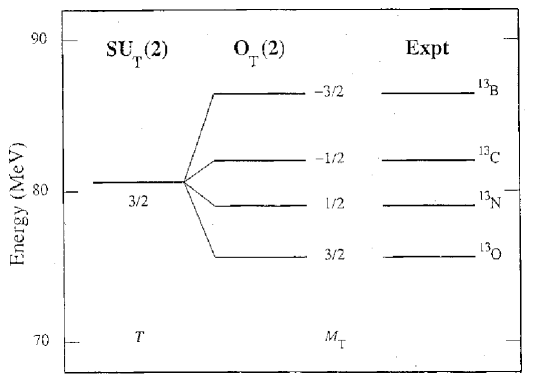
Figure 2: Binding energies of the $T=3/2$ isobaric analog states with angular momentum and parity $J^{\pi}=1/2^{-}$ in ¹³B, ¹³C, ¹³N, and ¹³O. The column on the left is obtained for an exact $SU_{T}(2)$ symmetry, which predicts states with different $M_{T}$ to be degenerate. The middle column is obtained in the case of an $SU_{T}(2)$ dynamical symmetry, equation (49) with parameters $a=80.59$, $b=-2.96$, and $c=-0.26$ MeV.

A less trivial example of dynamical-symmetry breaking is provided by the Gell-Mann–Okubo mass-splitting formula for elementary particles aGEL62 ; aOKU62 . The SU(3) model of Gell-Mann and Ne’eman aGEL64 classifies hadrons as SU(3) multiplets, that is, a given irreducible representation $(\lambda,\mu)$ of SU(3) of dimension $d$ contains $d$ particles. For example, the neutron and proton are placed in the eight dimensional representation (1,1), the so-called octet representation. Besides isospin $T$ a new quantum number is needed to fully classify the SU(3) states. This turns out to be an additive number $Y$, called hypercharge aELL79 , associated with the chain of algebras

$$\begin{array}[]{ccccccccc}SU(3)&\supset&U_{Y}(1)&\otimes&SU_{T}(2)&\supset&U_{Y}(1)&\otimes&SO_{T}(2)\\ |&&|&&|&&&&|\\ (\lambda,\mu)&&Y&&T&&&&M_{T}\end{array}$$ (50)

If one would assume SU(3) invariance, all particles in a multiplet would have the same mass, but since the experimental masses of other baryons differ from the nucleon masses by hundreds of MeV, the SU(3) symmetry clearly must be broken.

Dynamical symmetry breaking allows the baryon states to still be classified by (50). Following the procedure outlined above and keeping up to quadratic terms, one finds a mass operator of the form

$$\hat{M} = a+b\,{\cal C}_{1U_{Y}(1)}+c\,{\cal C}^{2}_{1U_{Y}(1)}+d\,{\cal C}_{2SU_{T}(2)}+e\,{\cal C}_{1SO_{T}(2)}+f\,{\cal C}^{2}_{1SO_{T}(2)}~{},$$ (51)

with eigenvalues

$$M(Y,T)=a+b\,Y+c\,Y^{2}+d\,T(T+1)+e\,M_{T}+f\,M_{T}^{2}~{}.$$ (52)

A further assumption regarding the SU(3) tensor character of the strong interaction aELL79 ; aGEL62 ; aOKU62 leads to a relation between $c$ and $d$ in (52), resulting in the Gell-Mann-Okubo mass formula

$$M^{\prime}(Y,T)=a+bY+d\left[T(T+1)-\frac{1}{4}Y^{2}\right]~{}.$$ (53)

In Figure 3 this process of successive dynamical-symmetry breaking is illustrated with the octet representation containing the neutron and the proton and the $\Lambda$, $\Sigma$, and $\Xi$ baryons.

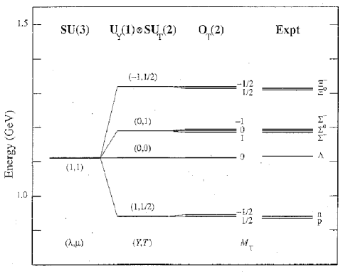
Figure 3: Mass spectrum of the SU(3) octet $(\lambda,\mu)=(1,1)$. The column on the left is obtained for an exact SU(3) symmetry, which predicts all masses to be the same, while the next two columns represent successive breakings of this symmetry in a dynamical manner. The column under $SO_{T}(2)$ is obtained with (53) with parameters $a=1111.3$, $b=-189.6$, $d=-39.9$, $e=-3.8$, and $f=0.9$ MeV.

Other hadrons are analogously classified using SU(3) as the dynamical algebra aELL79 ; aGEL64 . Other applications of the algebraic approach will be illustrated throughout these lecture notes, where the steps listed before are implemented for physical systems associated with $U(n)$ models. The algebraic approach, both in the sense we have defined here and in its generalizations to other fields of research, has become an important tool in the search for a unified description of physical phenomena. This is illustrated by Figure 3. The near equality of the neutron and proton masses suggested the existence of isospin multiplets, later confirmed at higher energies for other particles. To find a relationship between these multiplets, the $SU(3)$ dynamical algebra was proposed (and became the basis for the establishment of the quark model). This unification process can be continued: different $(\lambda,\mu)$ multiplets can be unified by means of higher-dimensional algebras such as $SU(4)$ aELL79 .

2.6 Superalgebras

To conclude the mathematical introduction, we now introduce the concept of superalgebra, which generalizes the algebras discussed in the previous sections and which is intimately related to the supersymmetry concept.

The mathematical structures based on the better known (Lie) algebras introduced before can be realized in terms of either bosons or fermions. A simple way to do this is to consider a system of bosons (fermions) which can be in $n$ ($m$) different states denoted by $\alpha,\alpha^{\prime},...$ ($\beta,\beta^{\prime},...$). They can be created or annhilated by the creation and annhilation operators $b^{\dagger}_{\alpha}$ ($a^{\dagger}_{\beta}$) and $b_{\alpha}$ ($a_{\beta}$), which satisfy

$$\begin{array}[]{lcl}[\,b_{\alpha},b^{\dagger}_{\alpha^{\prime}}]&=&\delta_{\alpha\alpha^{\prime}}~{},\\[4.30554pt] \{a_{\beta},a^{\dagger}_{\beta^{\prime}}\}&=&\delta_{\beta\beta^{\prime}}~{},\end{array}$$ (54)

with all other commutators (anticommutators) being zero. The bilinear products $({\cal G}^{\rm B}_{\rm B})_{\alpha\alpha^{\prime}}=b^{\dagger}_{\alpha}b_{\alpha^{\prime}}$ ($({\cal G}^{\rm F}_{\rm F})_{\beta\beta^{\prime}}=a^{\dagger}_{\beta}a_{\beta^{\prime}}$) can be shown to close under commutation

$$\begin{array}[]{lcl}[({\cal G}^{\rm B}_{\rm B})_{\alpha\alpha^{\prime}},({\cal G}^{\rm B}_{\rm B})_{\alpha^{\prime\prime}\alpha^{\prime\prime\prime}}]&=&({\cal G}^{\rm B}_{\rm B})_{\alpha\alpha^{\prime\prime}}\delta_{\alpha^{\prime}\alpha^{\prime\prime\prime}}-({\cal G}^{\rm B}_{\rm B})_{\alpha^{\prime}\alpha^{\prime\prime\prime}}\delta_{\alpha\alpha^{\prime\prime}}~{},\\[4.30554pt] [({\cal G}^{\rm F}_{\rm F})_{\beta\beta^{\prime}},({\cal G}^{\rm F}_{\rm F})_{\beta^{\prime\prime}\beta^{\prime\prime\prime}}]&=&({\cal G}^{\rm F}_{\rm F})_{\beta\beta^{\prime\prime}}\delta_{\beta^{\prime}\beta^{\prime\prime\prime}}-({\cal G}^{\rm F}_{\rm F})_{\beta^{\prime}\beta^{\prime\prime\prime}}\delta_{\beta\beta^{\prime\prime}}~{},\end{array}$$ (55)

and satisfy the Jacobi identity. So they define a Lie algebra of the general ${\rm U}^{\rm B}(n)$ (${\rm U}^{\rm F}(m)$) form. Since boson and fermion operators commute

$$[({\cal G}^{\rm B}_{\rm B})_{\alpha\alpha^{\prime}},({\cal G}^{\rm F}_{\rm F})_{\beta\beta^{\prime}}]=0~{}.$$ (56)

the set of operators ($({\cal G}^{\rm B}_{\rm B})_{\alpha\alpha^{\prime}},({\cal G}^{\rm F}_{\rm F})_{\beta\beta^{\prime}}$) define the direct-product algebra

$${\rm U}^{\rm B}(n)\otimes{\rm U}^{\rm F}(m)~{},$$ (57)

which is the dynamical algebra for the combined boson-fermion system (see Section 3.2).

The Hamiltonian of the boson, fermion or boson-fermion system can be built in terms of the bilinear products or generators of the corresponding dynamical algebras and separately conserves the boson and fermion numbers. The question arises as to whether one may define a generalized dynamical algebra where cross terms of the type $b^{\dagger}_{\alpha}a_{\beta}$ or $a^{\dagger}_{\beta}b_{\alpha}$ are included and, if so, to study the consequences of this generalization. From the standpoint of fundamental processes, where bosons correspond to forces (i.e. photons, gluons, etc.) and fermions to matter (i.e. electrons, nucleons, quarks, etc.), it may seem strange at first sight to consider symmetries which mix such intrinsically different particles. However, there have been numerous applications of these ideas in the last few years. These symmetries—known as supersymmetries—have given rise to schemes which hold promise in quantum field theory in regards to the unification of the fundamental interactions 4WES74 ; 4FAY77 ; 4NIE81 ; weinberg . In a different context, as mentioned in the introduction, the consideration of such “higher” symmetries in nuclear structure physics has provided a remarkable unification of the spectroscopic properties of quartets of neighboring nuclei FI , as we shall explain in the subsequent sections of these lecture notes. With this in mind, we shall consider the effects on the ${\rm U}^{\rm B}(n)\otimes{\rm U}^{\rm F}(m)$ model arising from embedding its dynamical algebra into a superalgebra.

To start our discussion of superalgebras, it is convenient to consider a schematic example, consisting of system formed by a single boson and a single (“spinless”) fermion, denoted by $b^{\dagger}$ and $a^{\dagger}$, respectively. In this case the bilinear products ${\cal G}^{\rm B}_{\rm B}=b^{\dagger}b$ and ${\cal G}^{\rm F}_{\rm F}=a^{\dagger}a$ each generate a U(1) algebra. Taken together, these generators conform the

$${\rm U}^{\rm B}(1)\otimes{\rm U}^{\rm F}(1)~{},$$ (58)

dynamical algebra, in analogy with the boson–fermion algebra mentioned above nueve . Let us now consider the introduction of the mixed terms $b^{\dagger}a$ and $a^{\dagger}b$. Computing the commutator of these operators, we find

$$[a^{\dagger}b,b^{\dagger}a]=a^{\dagger}bb^{\dagger}a-b^{\dagger}aa^{\dagger}b=a^{\dagger}a-b^{\dagger}b+2b^{\dagger}ba^{\dagger}a~{},$$ (59)

which does not close into the original set $(a^{\dagger}a,b^{\dagger}b,a^{\dagger}b,b^{\dagger}a)$. This means that the inclusion of the cross terms does not lead to a Lie algebra. We note, however, that the bilinear operators $b^{\dagger}a$ and $a^{\dagger}b$ do not behave like bosons, but rather as fermion operators, in contrast to $a^{\dagger}a$ and $b^{\dagger}b$, both of which have bosonic character (in the sense that, e.g., $a^{\dagger}_{i}a_{j}$ commutes with $a^{\dagger}_{k}a_{l})$. This suggests the separation of the generators in two sectors, the bosonic sector $(a^{\dagger}a,b^{\dagger}b)$ and the fermionic sector $(a^{\dagger}b,b^{\dagger}a)$. Computing the anticommutators of the latter, we find

$$\{a^{\dagger}b,a^{\dagger}b\}=0~{},\quad\{b^{\dagger}a,b^{\dagger}a\}=0~{},\quad\{a^{\dagger}b,b^{\dagger}a\}=a^{\dagger}a+b^{\dagger}b~{},$$ (60)

which indeed close into the same set. The commutators between the bosonic and fermionic sectors give

$$\begin{array}[]{lcl}[a^{\dagger}b,a^{\dagger}a]=-a^{\dagger}b~{},&&[b^{\dagger}a,a^{\dagger}a]=b^{\dagger}a~{},\\[4.30554pt] [a^{\dagger}b,b^{\dagger}b]=a^{\dagger}b~{},&&[b^{\dagger}a,b^{\dagger}b]=-b^{\dagger}a~{}.\end{array}$$ (61)

The operations defined in (60) and (61), together with the (in this case) trivial ${\rm U}^{\rm B}(1)\otimes{\rm U}^{\rm F}(1)$ commutators

$$[a^{\dagger}a,a^{\dagger}a]=[b^{\dagger}b,b^{\dagger}b]=[a^{\dagger}a,b^{\dagger}b]=0~{},$$ (62)

define the superalgebra U(1/1). To maintain the closure property for the enlarged set of generators belonging to the boson and fermion sectors, we are thus forced to include both commutators and anticommutators in the definition of a superalgebra. In general, superalgebras then involve boson-sector generators ${\hat{B}}_{i}$ and fermion-sector generators ${\hat{F}}_{j}$, satisfying the generalized relations

$$[{\hat{B}}_{i},{\hat{B}}_{j}]=\sum_{k}c^{k}_{ij}{\hat{B}}_{k}~{},\quad[{\hat{B}}_{i},{\hat{F}}_{j}]=\sum_{k}d^{k}_{ij}{\hat{F}}_{k}~{},\quad\{{\hat{F}}_{i},{\hat{F}}_{j}\}=\sum_{k}e^{k}_{ij}{\hat{B}}_{k}~{},$$ (63)

where $c^{k}_{ij}$, $d^{k}_{ij}$, and $e^{k}_{ij}$ are complex constants defining the structure of the superalgebra, hence their denomination as structure constants of the superalgebra 4BAR83 . We shall only be concerned in these lecture notes with superalgebras of the form ${\rm U}(n/m)$, where $n$ and $m$ denote the dimensions of the boson and fermion subalgebras ${\rm U}^{\rm B}(n)$ and ${\rm U}^{\rm F}(m)$. In Section 3 of these notes, we focus our attention on nuclear supersymmetry.

3 Nuclear Supersymmetry

Nuclear supersymmetry (n-SUSY) is a composite-particle phenomenon, linking the properties of bosonic and fermionic systems, framed in the context of the Interacting Boson Model of nuclear structure IBM . Composite particles, such as the $\alpha$-particle are known to behave as approximate bosons. As He atoms they become superfluid at low temperatures, an under certain conditions can also form Bose-Einstein condensates. At higher densities (or temperatures) the constituent fermions begin to be felt and the Pauli principle sets in. Odd-particle composite systems, on the other hand, behave as approximate fermions, which in the case of the Interacting Boson-Fermion Model are treated as a combination of bosons and an (ideal) fermion IBFM . In contrast to the theoretical construct of supersymmetric particle physics, where SUSY is postulated as a generalization of the Lorentz-Poincare invariance at a fundamental level, experimental evidence has been found for n-SUSY FI ; susy ; baha ; thesis ; tres ; pt195 ; au196 as we shall discuss below. Nuclear supersymmetry should not be confused with fundamental SUSY, which predicts the existence of supersymmetric particles, such as the photino and the selectron for which, up to now, no evidence has been found. If such particles exist, however, SUSY must be strongly broken, since large mass differences must exist among superpartners, or otherwise they would have been already detected. Competing SUSY models give rise to diverse mass predictions and are the basis for current superstring and brane theories weinberg ; cuatro . Nuclear supersymmetry, on the other hand, is a theory that establishes precise links among the spectroscopic properties of certain neighboring nuclei. Even-even and odd-odd nuclei are composite bosonic systems, while odd-A nuclei are fermionic. It is in this context that n-SUSY provides a theoretical framework where bosonic and fermionic systems are treated as members of the same supermultiplet baha . Nuclear supersymmetry treats the excitation spectra and transition intensities of the different nuclei as arising from a single Hamiltonian and a single set of transition operators. As we mentioned before, nuclear SUSY was originally postulated as a symmetry among pairs of nuclei FI ; susy ; baha , and was subsequently extended to nuclear quartets or “magic squares”, where odd-odd nuclei could be incorporated in a natural way quartet . Evidence for the existence of n-SUSY (albeit possibly significantly broken) grew over the years, specially for the quartet provided by the nuclei ¹⁹⁴Pt, ¹⁹⁵Au, ¹⁹⁵Pt and ¹⁹⁶Au, but only recently more systematic evidence was found. This was achieved by means of one-nucleon transfer reaction experiments leading to the odd-odd nucleus ¹⁹⁶Au, which, together with the other members of the SUSY quartet is considered to be the best example of n-SUSY in nature quartet ; pt195 ; au196 . We should point out, however, that while these experiments provided the first complete energy classification for ¹⁹⁶Au (which was found to be consistent with the theoretical predictions quartet ; pt195 ; au196 ), the reactions involved (¹⁹⁷Au$(\vec{d},t)$, ¹⁹⁷Au$(p,d)$ and ¹⁹⁸Hg$(\vec{d},\alpha)$) did not actually test directly the supersymmetric wave functions. Furthermore, whereas these new measurements are very exciting, the dynamical SUSY framework is so restrictive that there was little hope that other quartets could be found and used to verify the theory quartet ; pt195 ; au196 . In the following sections we emphasize two aspects of SUSY research. On the one hand we report on an ongoing investigation of one- and two-nucleon transfer reactions diez in the Pt-Au region that will more directly analyze the supersymmetric wave functions and measure new correlations which have not been tested up to now. On the other hand we discuss some ideas put forward several years ago, which question the need for dynamical symmetries in order for n-SUSY to exist once ; diecinueve . We thus propose a more general theoretical framework for nuclear supersymmetry. The combination of such a generalized form of supersymmetry and the transfer experiments now being carried out graw , could provide remarkable new correlations and a unifying theme in nuclear structure physics.

We first present a pedagogic review of dynamical (super)symmetries in even- and odd-mass nuclei, which is based in part on thesis . Next we discuss some new results on correlations between different transfer reactions and some perspectives for future work.

3.1 Dynamical Symmetries in Even-Even Nuclei

Dynamical supersymmetries were introduced FI in nuclear physics in 1980 by Franco Iachello in the context of the Interacting Boson Model (IBM) IBM and its extensions. The spectroscopy of atomic nuclei is characterized by the interplay between collective (bosonic) and single-particle (fermionic) degrees of freedom.

The IBM describes collective excitations in even-even nuclei in terms of a system of interacting monopole and quadrupole bosons with angular momentum $l=0,2$. The bosons are associated with the number of correlated proton and neutron pairs, and hence the number of bosons $N$ is half the number of valence nucleons. Since it is convenient to express the Hamiltonian and other operators of interest in second quantized form, we introduce creation, $s^{\dagger}$ and $d^{\dagger}_{m}$, and annihilation, $s$ and $d_{m}$, operators, which altogether can be denoted by $b^{\dagger}_{i}$ and $b_{i}$ with $i=l,m$ ($l=0,2$ and $-l\leq m\leq l$). The operators $b^{\dagger}_{i}$ and $b_{i}$ satisfy the commutation relations

$$[b_{i},b^{\dagger}_{j}]\;=\;\delta_{ij}~{},\hskip 28.45274pt[b^{\dagger}_{i},b^{\dagger}_{j}]\;=\;[b_{i},b_{j}]\;=\;0~{}.$$ (64)

The bilinear products

$$B_{ij}\;=\;b^{\dagger}_{i}b_{j}~{},$$ (65)

generate the algebra of $U(6)$ the unitary group in 6 dimensions

$$[B_{ij},B_{kl}]\;=\;B_{il}\,\delta_{jk}-B_{kj}\,\delta_{il}~{}.$$ (66)

We want to construct states and operators that transform according to irreducible representations of the rotation group (since the problem is rotationally invariant). The creation operators $b^{\dagger}_{i}$ transform by definition as irreducible tensors under rotation. However, the annihilation operators $b_{i}$ do not. It is an easy exercise to contruct operators that do transform appropriately

$$\tilde{b}_{lm}\;=\;(-)^{l-m}b_{l,-m}~{}.$$ (67)

The 36 generators of Eq. (65) can be rewritten in angular-momentum-coupled form as

$$[b^{\dagger}_{l}\times\tilde{b}_{l^{\prime}}]^{(L)}_{M}\;=\;\sum_{mm^{\prime}}\langle l,m,l^{\prime},m^{\prime}|L,M\rangle\,b^{\dagger}_{lm}\tilde{b}_{l^{\prime}m^{\prime}}~{}.$$ (68)

The one- and two-body Hamiltonian can be expressed in terms of the generators of $U(6)$ as

$$H = \sum_{l}\epsilon_{l}\sum_{m}b^{\dagger}_{lm}b_{lm}$$ (69)

$$+\sum_{L}\sum_{l_{1}l_{2}l_{3}l_{4}}u^{(L)}_{l_{1}l_{2}l_{3}l_{4}}\,[[b^{\dagger}_{l_{1}}\times\tilde{b}_{l_{2}}]^{(L)}\times[b^{\dagger}_{l_{3}}\times\tilde{b}_{l_{4}}]^{(L)}]^{(0)}~{}.$$

In general, the Hamiltonian has to be diagonalized numerically to obtain the energy eigenvalues and wave functions. There exist, however, special situations in which the eigenvalues can be obtained in closed, analytic form. These special solutions provide a framework in which energy spectra and other nuclear properties (such as quadrupole transitions and moments) can be interpreted in a qualitative way. These situations correspond to dynamical symmetries of the Hamiltonian IBM (see section 2.5).

The concept of dynamical symmetry has been shown to be a very useful tool in different branches of physics. A well-known example in nuclear physics is the Elliott $SU(3)$ model Elliott to describe the properties of light nuclei in the $sd$ shell. Another example is the $SU(3)$ flavor symmetry of Gell-Mann and Ne’eman aGEL64 to classify the baryons and mesons into flavor octets, decuplets and singlets and to describe their masses with the Gell-Mann-Okubo mass formula, as described in the previous sections.

The group structure of the IBM Hamiltonian is that of $G=U(6)$. Since nuclear states have good angular momentum, the rotation group in three dimensions $SO(3)$ should be included in all subgroup chains of $G$ IBM

$$U(6)\supset\left\{\begin{array}[]{l}U(5)\supset SO(5)\supset SO(3)~{},\\ SO(6)\supset SO(5)\supset SO(3)~{},\\ SU(3)\supset SO(3)~{}.\end{array}\right.$$ (73)

The three dynamical symmetries which correspond to the group chains in Eq. (73) are limiting cases of the IBM and are usually referred to as the $U(5)$ (vibrator), the $SU(3)$ (axially symmetric rotor) and the $SO(6)$ ($\gamma$-unstable rotor).

Here we consider a simplified form of the general expression of the IBM Hamiltonian of Eq. (69) that contains the main features of collective motion in nuclei

$$H\;=\;\epsilon\,\hat{n}_{d}-\kappa\,\hat{Q}(\chi)\cdot\hat{Q}(\chi)~{},$$ (74)

where $n_{d}$ counts the number of quadrupole bosons

$$\hat{n}_{d}\;=\;\sqrt{5}\,[d^{\dagger}\times\tilde{d}]^{(0)}\;=\;\sum_{m}d^{\dagger}_{m}d_{m}~{},$$ (75)

and $Q$ is the quadrupole operator

$$\hat{Q}_{m}(\chi)\;=\;[s^{\dagger}\times\tilde{d}+d^{\dagger}\times\tilde{s}+\chi\,d^{\dagger}\times\tilde{d}]^{(2)}_{m}~{}.$$ (76)

The three dynamical symmetries are recovered for different choices of the coefficients $\epsilon$, $\kappa$ and $\chi$. Since the IBM Hamiltonian conserves the number of bosons and is invariant under rotations, its eigenstates can be labeled by the total number of bosons $N$ and the angular momentum $L$.

In the absence of a quadrupole-quadrupole interaction $\kappa=0$, the Hamiltonian of Eq. (74) becomes proportional to the linear Casimir operator of $U(5)$

$$H_{1}\;=\;\epsilon\,\hat{n}_{d}\;=\;\epsilon\,{\cal C}_{1U(5)}~{}.$$ (77)

In addition to $N$, $L$ and $M$, the basis states can be labeled by the quantum numbers $n_{d}$ and $\tau$, which characterize the irreducible representations of $U(5)$ and $SO(5)$. Here $n_{d}$ represents the number of quadrupole bosons and $\tau$ the boson seniority. The eigenvalues of $H_{1}$ are given by the expectation value of the Casimir operator

$$E_{1}\;=\;\epsilon\,n_{d}~{}.$$ (78)

In this case, the energy spectrum is characterized by a series of multiplets, labeled by the number of quadrupole bosons, at a constant energy spacing which is typical for a vibrational nucleus.

For the quadrupole-quadrupole interaction, we can distinguish two situations in which the eigenvalue problem can be solved analytically. If $\chi=\mp\sqrt{7}/2$, the Hamiltonian has a $SU(3)$ dynamical symmetry

$$H_{2}\;=\;-\kappa\,\hat{Q}(\mp\sqrt{7}/2)\cdot\hat{Q}(\mp\sqrt{7}/2)\;=\;-\frac{1}{2}\kappa\left[{\cal C}_{2SU(3)}-\frac{3}{4}{\cal C}_{2SO(3)}\right]~{}.$$ (79)

In this case, the eigenstates can be labeled by $(\lambda,\mu)$ which characterize the irreducible representations of $SU(3)$. The eigenvalues are

$$E_{2}\;=\;-\frac{1}{2}\kappa\left[\lambda(\lambda+3)+\mu(\mu+3)+\lambda\mu)-\frac{3}{4}\kappa L(L+1)\right]~{}.$$ (80)

The energy spectrum is characterized by a series of bands, in which the energy spacing is proportional to $L(L+1)$, as in the rigid rotor model. The ground state band has $(\lambda,\mu)=(2N,0)$ and the first excited band $(2N-4,2)$ corresponds to a degenerate $\beta$ and $\gamma$ band. The sign of the coefficient $\chi$ is related to a prolate (-) or an oblate (+) deformation.

For $\chi=0$, the Hamiltonian has a $SO(6)$ dynamical symmetry

$$H_{3}\;=\;-\kappa\,\hat{Q}(0)\cdot\hat{Q}(0)\;=\;-\kappa\left[{\cal C}_{2SO(6)}-{\cal C}_{2SO(5)}\right]~{}.$$ (81)

The basis states are labeled by $\sigma$ and $\tau$ which characterize the irreducible representations of $SO(6)$ and $SO(5)$, respectively. Characteristic features of the energy spectrum

$$E_{3}\;=\;-\kappa\left[\sigma(\sigma+4)-\tau(\tau+3)\right]~{},$$ (82)

are the repeating patterns $L=0,2,4,2$ which is typical of the $\gamma$-unstable rotor.

For other choices of the coefficients, the Hamiltonian of Eq. (74) describes situations in between any of the dynamical symmetries which correspond to transitional regions, e.g. the Pt-Os isotopes exhibit a transition between a $\gamma$-unstable and a rigid rotor $SO(6)\leftrightarrow SU(3)$, the Sm isotopes between vibrational and rotational nuclei $U(5)\leftrightarrow SU(3)$, and the Ru isotopes between vibrational and $\gamma$-unstable nuclei $U(5)\leftrightarrow SO(6)$.

3.2 Dynamical Symmetries in Odd-A Nuclei

For odd-mass nuclei the IBM has been extended to include single-particle degrees of freedom IBFM . The Interacting Boson-Fermion Model (IBFM) has as its building blocks a set of $N$ bosons with $l=0,2$ and an odd nucleon (either a proton or a neutron) occupuying the single-particle orbits with angular momenta $j=j_{1},j_{2},\dots$. The components of the fermion angular momenta span the $m$-dimensional space of the group $U(m)$ with $m=\sum_{j}(2j+1)$.

We introduce, in addition to the boson creation $b^{\dagger}_{i}$ and annihilation $b_{i}$ operators for the collective degrees of freedom, fermion creation $a^{\dagger}_{i}$ and annihilation $a_{i}$ operators for the single-particle. The fermion operators satisfy anti-commutation relations

$$\{a_{i},a^{\dagger}_{j}\}\;=\;\delta_{ij}~{},\hskip 28.45274pt\{a^{\dagger}_{i},a^{\dagger}_{j}\}\;=\;\{a_{i},a_{j}\}\;=\;0~{}.$$ (83)

By construction the fermion operators commute with the boson operators. The bilinear products

$$A_{ij}\;=\;a^{\dagger}_{i}a_{j}~{},$$ (84)

generate the algebra of $U(m)$, the unitary group in $m$ dimensions

$$[A_{ij},A_{kl}]\;=\;A_{il}\,\delta_{jk}-A_{kj}\,\delta_{il}~{}.$$ (85)

For the mixed system of boson and fermion degrees of freedom we introduce angular-momentum-coupled generators as

$$B^{(L)}_{M}(l,l^{\prime})\;=\;[b^{\dagger}_{l}\times\tilde{b}_{l^{\prime}}]^{(L)}_{M}~{},\hskip 28.45274ptA^{(L)}_{M}(j,j^{\prime})\;=\;[a^{\dagger}_{j}\times\tilde{a}_{j^{\prime}}]^{(L)}_{M}~{},$$ (86)

where $\tilde{a}_{jm}$ is defined to be a spherical tensor operator

$$\tilde{a}_{jm}\;=\;(-)^{j-m}a_{j,-m}~{}.$$ (87)

The most general one- and two-body rotational invariant Hamiltonian of the IBFM can be written as

$$H\;=\;H_{B}+H_{F}+V_{BF}~{},$$ (88)

where $H_{B}$ is the IBM Hamiltonian of Eq. (69), $H_{F}$ is the fermion Hamiltonian

$$H_{F} = \sum_{j}\eta_{j}\sum_{m}a^{\dagger}_{jm}a_{jm}$$ (89)

$$+\sum_{L}\sum_{j_{1}j_{2}j_{3}j_{4}}v^{(L)}_{j_{1}j_{2}j_{3}j_{4}}\,[[a^{\dagger}_{j_{1}}\times\tilde{a}_{j_{2}}]^{(L)}\times[a^{\dagger}_{j_{3}}\times\tilde{a}_{j_{4}}]^{(L)}]^{(0)}~{},$$

and $B_{BF}$ the boson-fermion interaction

$$V_{BF} = \sum_{L}\sum_{l_{1}l_{2}j_{1}j_{2}}w^{(L)}_{l_{1}l_{2}j_{1}j_{2}}\,[[b^{\dagger}_{l_{1}}\times\tilde{b}_{l_{2}}]^{(L)}\times[a^{\dagger}_{j_{1}}\times\tilde{a}_{j_{2}}]^{(L)}]^{(0)}~{}.$$ (90)

The IBFM Hamiltonian has an interesting algebraic structure, that suggests the possible occurrence of dynamical symmetries in odd-A nuclei. Since in the IBFM odd-A nuclei are described in terms of a mixed system of interacting bosons and fermions, the concept of dynamical symmetries has to be generalized. Under the restriction, that both the boson and fermion states have good angular momentum, the respective group chains should contain the rotation group ($SO(3)$ for bosons and $SU(2)$ for fermions) as a subgroup

$$U^{B}(6)\supset\ldots\supset SO^{B}(3)~{},$$

$$U^{F}(m)\supset\ldots\supset SU^{F}(2)~{},$$ (91)

where we have introduced superscripts to distinguish between boson and fermion groups. If one of subgroups of $U^{B}(6)$ is isomorphic to one of the subgroups of $U^{F}(m)$, the boson and fermion group chains can be combined into a common boson-fermion group chain. When the Hamiltonian is written in terms of Casimir invariants of the combined boson-fermion group chain, a dynamical boson-fermion symmetry arises.

Among the many different possibilities, we consider two dynamical boson-fermion symmetries associated with the $SO(6)$ limit of the IBM. The first example discussed in the literature FI ; spin6 is the case of bosons with $SO(6)$ symmetry and the odd nucleon occupying a single-particle orbit with spin $j=3/2$. The relevant group chains are

$$U^{B}(6) \supset SO^{B}(6)\supset SO^{B}(5)\supset SO^{B}(3)~{},$$

$$U^{F}(4) \supset SU^{F}(4)\supset Sp^{F}(4)\supset SU^{F}(2)~{}.$$ (92)

Since $SO(6)$ and $SU(4)$ are isomorphic, the boson and fermion group chains can be combined into

$$U^{B}(6)\otimes U^{F}(4) \supset SO^{B}(6)\otimes SU^{F}(4)$$ (93)

$$\supset Spin(6)\supset Spin(5)\supset Spin(3)~{}.$$

The spinor groups $Spin(n)$ are the universal covering groups of the orthogonal groups $SO(n)$, with $Spin(6)\sim SU(4)$, $Spin(5)\sim Sp(4)$ and $Spin(3)\sim SU(2)$. The generators of the spinor groups consist of the sum of a boson and a fermion part. For example, for the quadrupole operator we have

$$\hat{Q}_{m}\;=\;[s^{\dagger}\times\tilde{d}+d^{\dagger}\times\tilde{s}]^{(2)}_{m}+[a^{\dagger}_{3/2}\times\tilde{a}_{3/2}]^{(2)}_{m}~{}.$$ (94)

We consider a simple quadrupole-quadrupole interaction which, just as for the $SO(6)$ limit of the IBM, can be written as the difference of two Casimir invariants

$$H\;=\;-\kappa\,\hat{Q}\cdot\hat{Q}\;=\;-\kappa\left[{\cal C}_{2Spin(6)}-{\cal C}_{2Spin(5)}\right]~{}.$$ (95)

The basis states are classified by $(\sigma_{1},\sigma_{2},\sigma_{3})$, $(\tau_{1},\tau_{2})$ and $J$ which label the irreducible representations of the spinor groups $Spin(6)$, $Spin(5)$ and $Spin(3)$. The energy spectrum is obtained from the expectation value of the Casimir invariants of the spinor groups

$$E\;=\;-\kappa\left[\sigma_{1}(\sigma_{1}+4)+\sigma_{2}(\sigma_{2}+2)+\sigma_{3}^{2}-\tau_{1}(\tau_{1}+3)-\tau_{2}(\tau_{2}+1)\right]~{}.$$ (96)

The mass region of the Os-Ir-Pt-Au nuclei, where the even-even Pt nuclei are well described by the $SO(6)$ limit of the IBM and the odd proton mainly occupies the $d_{3/2}$ shell, seems to provide experimental examples of this symmetry, e.g. ^191,193Ir and ^193,195Au.

The concept of dynamical boson-fermion symmetries is not restricted to cases in which the odd nucleon occupies only a single-$j$ orbit. The first example of a multi-$j$ case discussed in the literature baha is that of a dynamical boson-fermion symmetry associated with the $SO(6)$ limit and the odd nucleon occupying single-particle orbits with spin $j=1/2$, 3/2, 5/2. In this case, the fermion space is decomposed into a pseudo-orbital part with $k=0,2$ and a pseudo-spin part with $s=1/2$ corresponding to the group reduction

$$U^{F}(12)\supset U^{F}(6)\otimes U^{F}(2)\supset\left\{\begin{array}[]{c}U^{F}(5)\otimes U^{F}(2)~{},\\ SU^{F}(3)\otimes U^{F}(2)~{},\\ SO^{F}(6)\otimes U^{F}(2)~{}.\end{array}\right.$$ (100)

Since the pseudo-orbital angular momentum $k$ has the same values as the angular momentum of the $s$- and $d$- bosons of the IBM, it is clear that the pseudo-orbital part can be combined with all three dynamical symmetries of the IBM.

$$U^{B}(6)\supset\left\{\begin{array}[]{c}U^{B}(5)~{},\\ SU^{B}(3)~{},\\ SO^{B}(6)~{}.\end{array}\right.$$ (104)

into a dynamical boson-fermion symmetry. The case, in which the bosons have $SO(6)$ symmetry is of particular interest, since the negative parity states in Pt with the odd neutron occupying the $3p_{1/2}$, $3p_{3/2}$ and $3f_{5/2}$ orbits have been suggested as possible experimental examples of a multi-$j$ boson-fermion symmetry. In this case, the relevant boson-fermion group chain is

$$U^{B}(6)\otimes U^{F}(12) \supset U^{B}(6)\otimes U^{F}(6)\otimes U^{F}(2)$$ (105)

$$\supset U^{BF}(6)\otimes U^{F}(2)$$

$$\supset SO^{BF}(6)\otimes U^{F}(2)$$

$$\supset SO^{BF}(5)\otimes U^{F}(2)$$

$$\supset SO^{BF}(3)\otimes SU^{F}(2)$$

$$\supset SU(2)~{}.$$

Just as in the first example for the spinor groups, the generators of the boson-fermion groups consist of the sum of a boson and a fermion part, e.g. the quadrupole operator is now written as

$$\hat{Q}_{m}\;=\;[s^{\dagger}\times\tilde{d}+d^{\dagger}\times\tilde{s}]^{(2)}_{m} + \sqrt{\frac{4}{5}}\,[a^{\dagger}_{3/2}\times\tilde{a}_{1/2}-a^{\dagger}_{1/2}\times\tilde{a}_{3/2}]^{(2)}_{m}$$ (106)

$$+ \sqrt{\frac{6}{5}}\,[a^{\dagger}_{5/2}\times\tilde{a}_{1/2}+a^{\dagger}_{1/2}\times\tilde{a}_{5/2}]^{(2)}_{m}~{}.$$

Also in this case, the quadrupole-quadrupole interaction can be written as the difference of two Casimir invariants

$$H\;=\;-\kappa\,\hat{Q}\cdot\hat{Q}\;=\;-\kappa\left[{\cal C}_{2SO^{BF}(6)}-{\cal C}_{2SO^{BF}(5)}\right]~{}.$$ (107)

The basis states are classified by $(\sigma_{1},\sigma_{2},\sigma_{3})$, $(\tau_{1},\tau_{2})$ and $L$ which label the irreducible representations of the boson-fermion groups $SO^{BF}(6)$, $SO^{BF}(5)$ and $SO^{BF}(3)$. Although the labels are the same as for the previous case, the allowed values are different. The total angular momentum is given by $\vec{J}=\vec{L}+\vec{s}$. The energy spectrum is given by

$$E\;=\;-\kappa\left[\sigma_{1}(\sigma_{1}+4)+\sigma_{2}(\sigma_{2}+2)+\sigma_{3}^{2}-\tau_{1}(\tau_{1}+3)-\tau_{2}(\tau_{2}+1)\right]~{}.$$ (108)

The mass region of the Os-Ir-Pt-Au nuclei, where the even-even Pt nuclei are well described by the $SO(6)$ limit of the IBM and the odd neutron mainly occupies the negative parity orbits $3p_{1/2}$, $3p_{3/2}$ and $3f_{5/2}$ provides experimental examples of this symmetry, in particular the nucleus ¹⁹⁵Pt baha ; BI ; sun ; pt195

3.3 Dynamical Supersymmetries

Boson-fermion symmetries can further be extended by introducing the concept of supersymmetries susy , in which states in both even-even and odd-even nuclei are treated in a single framework. In the previous section, we have discussed the symmetry properties of a mixed system of boson and fermion degrees of freedom for a fixed number of bosons $N$ and one fermion $M=1$. The operators $B_{ij}$ and $A_{ij}$

$$B_{ij}\;=\;b^{\dagger}_{i}b_{j}~{},\hskip 28.45274ptA_{ij}\;=\;a^{\dagger}_{i}a_{j}~{},$$ (109)

which generate the Lie algebra of the symmetry group $U^{B}(6)\otimes U^{F}(m)$ of the IBFM, can only change bosons into bosons and fermions into fermions. The number of bosons $N$ and the number of fermions $M$ are both conserved quantities. As explained in Section 2.6, in addition to $B_{ij}$ and $A_{ij}$, one can introduce operators that change a boson into a fermion and vice versa

$$F_{ij}\;=\;b^{\dagger}_{i}a_{j}~{},\hskip 28.45274ptG_{ij}\;=\;a^{\dagger}_{i}b_{j}~{}.$$ (110)

The enlarged set of operators $B_{ij}$, $A_{ij}$, $F_{ij}$ and $G_{ij}$ forms a closed algebra which consists of both commutation and anticommutation relations

$$\,[B_{ij},B_{kl}] = B_{il}\,\delta_{jk}-B_{kj}\,\delta_{il}~{},$$

$$\,[B_{ij},A_{kl}] = 0~{},$$

$$\,[B_{ij},F_{kl}] = F_{il}\,\delta_{jk}~{},$$

$$\,[B_{ij},G_{kl}] = -G_{kj}\,\delta_{il}~{},$$

$$\,[A_{ij},A_{kl}] = A_{il}\,\delta_{jk}-A_{kj}\,\delta_{il}~{},$$

$$\,[A_{ij},F_{kl}] = -F_{kj}\,\delta_{il}~{},$$

$$\,[A_{ij},G_{kl}] = G_{il}\,\delta_{jk}~{},$$

$$\{F_{ij},F_{kl}\} = 0~{},$$

$$\{F_{ij},G_{kl}\} = B_{il}\,\delta_{jk}+A_{kj}\,\delta_{il}~{},$$

$$\{G_{ij},G_{kl}\} = 0~{}.$$ (111)

This algebra can be identified with that of the graded Lie group $U(6/m)$. It provides an elegant scheme in which the IBM and IBFM can be unified into a single framework susy

$$U(6/m)\supset U^{B}(6)\otimes U^{F}(m)~{}.$$ (112)

In this supersymmetric framework, even-even and odd-mass nuclei form the members of a supermultiplet which is characterized by ${\cal N}=N+M$, i.e. the total number of bosons and fermions. Supersymmetry thus distinguishes itself from “normal” symmetries in that it includes, in addition to transformations among fermions and among bosons, also transformations that change a boson into a fermion and vice versa.

The Os-Ir-Pt-Au mass region provides ample experimental evidence for the occurrence of dynamical (super)symmetries in nuclei. The even-even nuclei ^194,196Pt are the standard examples of the $SO(6)$ limit of the IBM so6 and the odd proton, in first approximation, occupies the single-particle level $2d_{3/2}$. In this special case, the boson and fermion groups can be combined into spinor groups, and the odd-proton nuclei ^191,193Ir and ^193,195Au were suggested as examples of the $Spin(6)$ limit FI . The appropriate extension to a supersymmetry is by means of the graded Lie group $U(6/4)$

$$U(6/4)\supset U^{B}(6)\otimes U^{F}(4) \supset SO^{B}(6)\otimes SU^{F}(4)$$ (113)

$$\supset Spin(6)\supset Spin(5)\supset Spin(3)\supset Spin(2)~{}.$$

The pairs of nuclei ¹⁹⁰Os - ¹⁹¹Ir, ¹⁹²Os - ¹⁹³Ir, ¹⁹²Pt - ¹⁹³Au and ¹⁹⁴Pt - ¹⁹⁵Au have been analyzed as examples of a $U(6/4)$ supersymmetry susy .

$\begin{array}[]{c}\begin{turn}{-90.0}\includegraphics[height=284.52756pt]{OromanaFrank_fig3a.eps}\end{turn}\\ \hskip 17.07182pt\begin{turn}{90.0}\includegraphics[height=298.75394pt]{OromanaFrank_fig3b.eps}\end{turn}\end{array}$

Figure 4: Example of a $U(6/4)$ supersymmetry

Another example of a dynamical supersymmetry in this mass region is that of the Pt nuclei. The even-even isotopes are well described by the $SO(6)$ limit of the IBM and the odd neutron mainly occupies the negative parity orbits $3p_{1/2}$, $3p_{3/2}$ and $3f_{5/2}$. In this case, the graded Lie group is $U(6/12)$

$$U(6/12)\supset U^{B}(6)\otimes U^{F}(12) \supset U^{B}(6)\otimes U^{F}(6)\otimes U^{F}(2)$$ (114)

$$\supset U^{BF}(6)\otimes U^{F}(2)$$

$$\supset SO^{BF}(6)\otimes U^{F}(2)$$

$$\supset SO^{BF}(5)\otimes U^{F}(2)$$

$$\supset SO^{BF}(3)\otimes SU^{F}(2)$$

$$\supset SU(2)~{}.$$

The odd-neutron nucleus ¹⁹⁵Pt, together with ¹⁹⁴Pt, were studied as an example of a $U(6/12)$ supersymmetry baha ; BI ; sun .

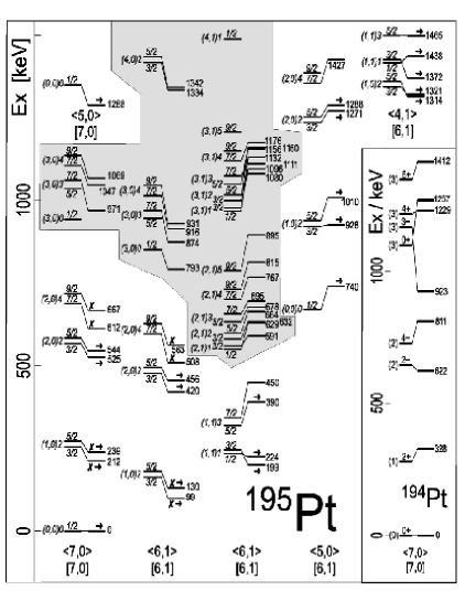
Figure 5: Example of a $U(6/12)$ supersymmetry

3.4 Dynamical Neutron-Proton Supersymmetries

As we have seen in the previous section, the mass region $A\sim 190$ has been a rich source of possible empirical evidence for the existence of (super)symmetries in nuclei. The pairs of nuclei ¹⁹⁰Os - ¹⁹¹Ir, ¹⁹²Os - ¹⁹³Ir, ¹⁹²Pt - ¹⁹³Au and ¹⁹⁴Pt - ¹⁹⁵Au have been analyzed as examples of a $U(6/4)$ supersymmetry susy , and the nuclei ¹⁹⁴Pt - ¹⁹⁵Pt as an example of a $U(6/12)$ supersymmetry baha . These ideas were later extended to the case where neutron and proton bosons are distinguished quartet , predicting in this way a correlation among quartets of nuclei, consisting of an even-even, an odd-proton, an odd-neutron and an odd-odd nucleus. The best experimental example of such a quartet with $U(6/12)_{\nu}\otimes U(6/4)_{\pi}$ supersymmetry is provided by the nuclei ¹⁹⁴Pt, ¹⁹⁵Au, ¹⁹⁵Pt and ¹⁹⁶Au.

$$\begin{array}[]{ccccc}\mbox{even-even}&&&&\mbox{odd-even}\\ N_{\nu}+1,N_{\pi}+1&&&&N_{\nu},N_{\pi}+1,j_{\nu}\\ &&&&\\ &{}^{194}_{78}\mbox{Pt}_{116}&\leftrightarrow&{}^{195}_{78}\mbox{Pt}_{117}&\\ &&&&\\ &\updownarrow&&\updownarrow&\\ &&&&\\ &{}^{195}_{79}\mbox{Au}_{116}&\hskip 28.45274pt\leftrightarrow&{}^{196}_{79}\mbox{Au}_{117}&\\ &&&&\\ \mbox{even-odd}&&&&\mbox{odd-odd}\\ N_{\nu}+1,N_{\pi},j_{\pi}&&&&N_{\nu},N_{\pi},j_{\nu},j_{\pi}\end{array}$$ (126)

In previous sections, we have used a schematic Hamiltonian consisting only of a quadrupole-quadrupole interaction to discuss the different dynamical symmetries. In general, a dynamical (super)symmetry arises whenever the Hamiltonian is expressed in terms of the Casimir invariants of the subgroups in a group chain. The relevant subgroup chain of $U(6/12)_{\nu}\otimes U(6/4)_{\pi}$ for the Pt and Au nuclei is given by quartet

$$U(6/12)_{\nu}\otimes U(6/4)_{\pi} \supset U^{B_{\nu}}(6)\otimes U^{F_{\nu}}(12)\otimes U^{B_{\pi}}(6)\otimes U^{F_{\pi}}(4)$$ (127)

$$\supset U^{B}(6)\otimes U^{F_{\nu}}(6)\otimes U^{F_{\nu}}(2)\otimes U^{F_{\pi}}(4)$$

$$\supset U^{BF_{\nu}}(6)\otimes U^{F_{\nu}}(2)\otimes U^{F_{\pi}}(4)$$

$$\supset SO^{BF_{\nu}}(6)\otimes U^{F_{\nu}}(2)\otimes SU^{F_{\pi}}(4)$$

$$\supset Spin(6)\otimes U^{F_{\nu}}(2)$$

$$\supset Spin(5)\otimes U^{F_{\nu}}(2)$$

$$\supset Spin(3)\otimes SU^{F_{\nu}}(2)$$

$$\supset SU(2)~{}.$$

In this case, the Hamiltonian

$$H = \alpha\,C_{2U^{BF_{\nu}}(6)}+\beta\,C_{2SO^{BF_{\nu}}(6)}+\gamma\,C_{2Spin(6)}$$ (128)

$$+\delta\,C_{2Spin(5)}+\epsilon\,C_{2Spin(3)}+\eta\,C_{2SU(2)}~{},$$

describes simultaneously the excitation spectra of the quartet of nuclei. Here we have neglected terms that only contribute to binding energies. The energy spectrum is given by the eigenvalues of the Casimir operators

$$E = \alpha\,\left[N_{1}(N_{1}+5)+N_{2}(N_{2}+3)+N_{3}(N_{3}+1)\right]$$ (129)

$$+\beta\,\left[\Sigma_{1}(\Sigma_{1}+4)+\Sigma_{2}(\Sigma_{2}+2)+\Sigma_{3}^{2}\right]$$

$$+\gamma\,\left[\sigma_{1}(\sigma_{1}+4)+\sigma_{2}(\sigma_{2}+2)+\sigma_{3}^{2}\right]$$

$$+\delta\,\left[\tau_{1}(\tau_{1}+3)+\tau_{2}(\tau_{2}+1)\right]+\epsilon\,J(J+1)+\eta\,L(L+1)~{}.$$

The coefficients $\alpha$, $\beta$, $\gamma$, $\delta$, $\epsilon$ and $\eta$ have been determined in a simultaneous fit of the excitation energies of the four nuclei of Eq. (126) au196 .

The supersymmetric classification of nuclear levels in the Pt and Au isotopes has been re-examined by taking advantage of the significant improvements in experimental capabilities developed in the last decade. High resolution transfer experiments with protons and polarized deuterons have strengthened the evidence for the existence of supersymmetry in atomic nuclei. The experiments include high resolution transfer experiments to ¹⁹⁶Au at TU/LMU München tres ; pt195 , and in-beam gamma ray and conversion electron spectroscopy following the reactions ¹⁹⁶Pt$(d,2n)$ and ¹⁹⁶Pt$(p,n)$ at the cyclotrons of the PSI and Bonn au196 . These studies have achieved an improved classification of states in ¹⁹⁵Pt and ¹⁹⁶Au which give further support to the original ideas baha ; sun ; quartet and extend and refine previous experimental work mauthofer ; jolie ; rotbard in this research area.

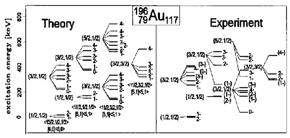
Figure 6: Comparison between the energy spectrum of the negative parity levels in the odd-odd nucleus ¹⁹⁶Au and that obtained for the $U(6/12)_{\nu}\otimes U(6/4)_{\pi}$ supersymmetry using Eq. (129) with $\alpha=52.5$, $\beta=8.7$, $\gamma=-53.9$, $\delta=48.8$, $\epsilon=8.8$ and $\eta=4.5$ in keV.

In analogy to the case of dynamical symmetries, in a dynamical supersymmetry closed expressions can be derived for energies, as well as selection rules and intensities for electromagnetic transitions and single-particle transfer reactions. While a simultaneous description and classification of these observables in terms of the $U(6/12)_{\nu}\otimes U(6/4)_{\pi}$ supersymmetry has been shown to be fulfilled to a good approximation for the quartet of nuclei ¹⁹⁴Pt, ¹⁹⁵Au, ¹⁹⁵Pt and ¹⁹⁶Au, there are important predictions still not fully verified by experiments. These tests involve the transfer reaction intensities among the supersymmetric partners. In the next section we concentrate on the latter and, in particular, on the one-proton transfer reactions ¹⁹⁴Pt $\rightarrow$ ¹⁹⁵Au and ¹⁹⁵Pt $\rightarrow$ ¹⁹⁶Au.

3.5 One-nucleon transfer reactions

The single-particle transfer operator that is commonly used in the Interacting Boson-Fermion Model (IBFM), has been derived in the seniority scheme olaf . Although strictly speaking this derivation is only valid in the vibrational regime, it has been used for deformed nuclei as well. An alternative method is based on symmetry considerations. It consists in expressing the single-particle transfer operator in terms of tensor operators under the subgroups that appear in the group chain of a dynamical (super)symmetry spin6 ; BI ; barea . The single-particle transfer between different members of the same supermultiplet provides an important test of supersymmetries, since it involves the transformation of a boson into a fermion or vice versa, but it conserves the total number of bosons plus fermions.

The operators that describe one-proton transfer reactions in the $U(6/12)_{\nu}\otimes U(6/4)_{\pi}$ supersymmetry are given by barea

$$T_{1,m}^{(\frac{1}{2},\frac{1}{2},-\frac{1}{2}),(\frac{1}{2},\frac{1}{2}),\frac{3}{2}} = -\sqrt{\frac{1}{6}}\left(\tilde{s}_{\pi}\times a^{\dagger}_{\pi,\frac{3}{2}}\right)^{(\frac{3}{2})}_{m}+\sqrt{\frac{5}{6}}\left(\tilde{d}_{\pi}\times a^{\dagger}_{\pi,\frac{3}{2}}\right)^{(\frac{3}{2})}_{m}~{},$$

$$T_{2,m}^{(\frac{3}{2},\frac{1}{2},\frac{1}{2}),(\frac{1}{2},\frac{1}{2}),\frac{3}{2}} = \sqrt{\frac{5}{6}}\left(\tilde{s}_{\pi}\times a^{\dagger}_{\pi,\frac{3}{2}}\right)^{(\frac{3}{2})}_{m}+\sqrt{\frac{1}{6}}\left(\tilde{d}_{\pi}\times a^{\dagger}_{\pi,\frac{3}{2}}\right)^{(\frac{3}{2})}_{m}~{}.$$ (130)

The operators $T_{1}$ and $T_{2}$ are, by construction, tensor operators under $Spin(6)$, $Spin(5)$ and $Spin(3)$ barea . The upper indices $(\sigma_{1},\sigma_{2},\sigma_{3})$, $(\tau_{1},\tau_{2})$, $J$ specify the tensorial properties under $Spin(6)$, $Spin(5)$ and $Spin(3)$. The use of tensor operators to describe single-particle transfer reactions in the supersymmetry scheme has the advantage of giving rise to selection rules and closed expressions for the spectroscopic factors.

Figure 7: Allowed one-proton transfer reactions for ¹⁹⁴Pt $\rightarrow$ ¹⁹⁵Au. The spectroscopic factors are normalized to 100 for the ground state to ground state transition for the operators $T_{1}/T_{2}$.

Fig. 7 shows the allowed transitions for the transfer operators of Eq. (130) that describe the one-proton transfer from the ground state $|(N+2,0,0)$, $(0,0)$, $0\rangle$ of the even-even nucleus ¹⁹⁴Pt to the even-odd nucleus ¹⁹⁵Au belonging to the supermultiplet $[N_{\nu}+1\}\otimes[N_{\pi}+1\}_{\pi}$. The number of bosons $N$ is taken to be the number of bosons in the odd-odd nucleus ¹⁹⁶Au: $N=N_{\nu}+N_{\pi}$ ($=5$). The operators $T_{1}$ and $T_{2}$ have the same transformation character under $Spin(5)$ and $Spin(3)$, and therefore can only excite states with $(\tau_{1},\tau_{2})=(\frac{1}{2},\frac{1}{2})$ and $J=\frac{3}{2}$. However, they differ in their $Spin(6)$ selection rules. Whereas $T_{1}$ can only excite the ground state of the even-odd nucleus with $(\sigma_{1},\sigma_{2},\sigma_{3})=(N+\frac{3}{2},\frac{1}{2},\frac{1}{2})$, the operator $T_{2}$ also allows the transfer to an excited state with $(N+\frac{1}{2},\frac{1}{2},-\frac{1}{2})$. The ratio of the intensities is given by barea

$$R_{1} = \frac{I_{\rm gs\rightarrow exc}}{I_{\rm gs\rightarrow gs}}\;=\;0~{},$$

$$R_{2} = \frac{I_{\rm gs\rightarrow exc}}{I_{\rm gs\rightarrow gs}}\;=\;\frac{9(N+1)(N+5)}{4(N+6)^{2}}~{},$$ (131)

for $T_{1}$ and $T_{2}$, respectively. In the case of the one-proton transfer ¹⁹⁴Pt $\rightarrow$ ¹⁹⁵Au, the second ratio is given by $R_{2}=1.12$ ($N=5$).

The available experimental data from the proton stripping reactions ¹⁹⁴Pt$(\alpha,t)^{195}$Au and ¹⁹⁴Pt$(^{3}$He$,d)^{195}$Au munger shows that the $J=3/2$ ground state of ¹⁹⁵Au is excited strongly with $C^{2}S=0.175$, whereas the first excited $J=3/2$ state is excited weakly with $C^{2}S=0.019$. In the SUSY scheme, the latter state is assigned as a member of the ground state band with $(\tau_{1},\tau_{2})=(5/2,1/2)$. Therefore the one proton transfer to this state is forbidden by the $Spin(5)$ selection rule of the tensor operators of Eq. (130). The relatively small strength to excited $J=3/2$ states suggests that the operator $T_{1}$ of Eq. (130) can be used to describe the data.

Figure 8: As Fig. 7, but for ¹⁹⁵Pt $\rightarrow$ ¹⁹⁶Au.

In Fig. 8 we show the allowed transitions for the one-proton transfer from the ground state $|(N+2,0,0),(0,0),0,\frac{1}{2}\rangle$ of the odd-even nucleus ¹⁹⁵Pt to the odd-odd nucleus ¹⁹⁶Au. Also in this case, the operator $T_{1}$ only excites the ground state doublet of ¹⁹⁶Au with $(\sigma_{1},\sigma_{2},\sigma_{3})=(N+\frac{3}{2},\frac{1}{2},\frac{1}{2})$, $(\tau_{1},\tau_{2})=(\frac{1}{2},\frac{1}{2})$, $J=\frac{3}{2}$ and $L=J\pm\frac{1}{2}$, whereas $T_{2}$ also populates the excited state with $(N+\frac{1}{2},\frac{1}{2},-\frac{1}{2})$. The ratio of the intensities is the same as for the ¹⁹⁴Pt $\rightarrow$ ¹⁹⁵Au transfer reaction

$$R_{1}(^{195}\mbox{Pt}\rightarrow^{196}\mbox{Au}) = R_{1}(^{194}\mbox{Pt}\rightarrow^{195}\mbox{Au})\;=\;0~{},$$

$$R_{2}(^{195}\mbox{Pt}\rightarrow^{196}\mbox{Au}) = R_{2}(^{194}\mbox{Pt}\rightarrow^{195}\mbox{Au})\;=\;\frac{9(N+1)(N+5)}{4(N+6)^{2}}~{}.$$ (132)

This is direct consequence of the supersymmetry. Just as the energies and the electromagnetic transition rates of the supersymmetric quartet of nuclei were calculated with the same form of the Hamiltonian and the transition operator, here we have extended this idea to the one-proton transfer reactions. We find definite predictions for the spectroscopic factors of the ¹⁹⁵Pt $\rightarrow$ ¹⁹⁶Au transfer reactions, which can be tested experimentally. To the best of our knowledge, there are no data available for this reaction.

For the one-neutron transfer reactions there exists a similar situation. The available experimental data from the neutron stripping reactions ¹⁹⁴Pt $(d,p)^{195}$Pt sheline can be used to determine the appropriate form of the one-neutron transfer operator BI , which then can be used to predict the spectroscopic factors for the transfer reaction ¹⁹⁵Au $\rightarrow$ ¹⁹⁶Au. We believe that, as a consequence of the supersymmetry classification, a number of additional correlations exist for transfer reactions between different pairs of nuclei. This would be the first time that such relations are predicted for nuclear reactions, something which may provide a challenge and motivation for future experiments.

3.6 New Experiments

The great majority of tests carried out for the nuclear supersymmetry involves one-nucleon transfer experiments such as ¹⁹⁷Au$(\vec{d},t)^{196}$Au and ¹⁹⁶Pt $(\vec{d},t)^{195}$Pt that, in first approximation, are formulated using a transfer operator of the form $a^{\dagger}_{\nu}$. These reactions are very useful to measure energies, angular momenta and parity of the residual nucleus. However, they do not test correlations present in the quartet’s wave functions as the case for one-nucleon transfer reactions inside the supermultiplet (see previous section). The latter reactions do provide a direct test of the fermionic sector (operators $F_{ij}$ and $G_{ij}$ of Eq. (110)) of the graded Lie Algebras $U_{\nu}(6/12)$ and $U_{\pi}(6/4)$.

New experimental facilities and detection techniques tres ; pt195 ; au196 ; wirth offer a unique opportunity for analyzing the supersymmetry classification in greater detail graw . In reference barea we pointed out a symmetry route for the theoretical analysis of such reactions, via the use of tensor operators of the algebras and superalgebras. An alternative route is the use of a semi-microscopic approach where projection techniques starting from the original nucleon pairs lead to specific forms for the operators olaf ; quince which, however, are only strictly valid in the generalized seniority regime dieciseis . The former and latter routes may be related by a consistent-operator approach, where the Hamiltonian exchange operators are made to be consistent with the one-nucleon transfer operator implying that the exchange term in the boson-fermion Hamiltonian can be viewed as an internal exchange reaction among the nucleon and the nucleon pairs. In addition to these experiments, ongoing research explores the possibility of testing SUSY through new transfer reactions. The two-nucleon transfer $(\alpha,\vec{d})$ and $(\vec{d},\alpha)$ reactions probe neutron-proton correlations in the nuclear wave function and constitutes a very stringent test of the supersymmetry classification.

In particular, the ¹⁹⁴Pt$(\alpha,\vec{d})^{196}$Au reaction involves nuclei belonging to the same supermultiplet. Therefore this process can be described by a combination of the fermionic generators the superalgebra (see Eq. (110)). Likewise, the reaction ¹⁹⁵Pt$(^{3}$He$,t)^{195}$Au is expressible in terms of the fermionic operators which, in this case, is associated to the beta-decay operator dieciocho . These reactions and their relation to single-nucleon transfer experiments raise the exciting possibility of testing direct correlations among transfer reaction spectroscopic factors in different nuclei, predicted by the supersymmetric classification of the magic quartet. A preliminary report on these analyses was presented in Ref. diez .

3.7 SUSY without Dynamical Symmetry

$\begin{array}[]{lr}\includegraphics[height=284.52756pt,width=156.49014pt]{OromanaFrank_fig8a.eps}&\includegraphics[height=284.52756pt,width=156.49014pt]{OromanaFrank_fig8b.eps}\end{array}$

Figure 9: Experimental and calculated positive-parity states in ^102-108Ru and negative-parity states in ^103-109Rh once .

The concept of dynamical algebra (not to be confused with that of dynamical symmetry) implies a generalization of the concept of symmetry algebra, as explained in Section 2.2. If $G$ is the dynamical algebra of a system, all physical states considered belong to a single irreducible representation (IR) of $G$. (In a symmetry algebra, in contrast, each set of degenerate states of the system is associated to an IR). The best known examples of a dynamical algebra are perhaps $SO(4,2)$ for the hydrogen atom and the $U(6)$ IBM algebra for even-even nuclei. A consequence of having a dynamical algebra associated to a system is that all sates can be reached using the algebra’s generators or, equivalently, all physical operators can be expressed in terms of these operators nueve . Naturally, the same Hamiltonian and the same transition operators are employed for all states in the system. To further clarify this point, it is certainly true that a single $H$ and a single set of operators are associated to a given even-even nucleus in the IBM framework, expressed in terms of the $U(6)$ (dynamical algebra) generators. It doesn’t matter whether this Hamiltonian can be expressed or not in terms of the generators of a single chain of groups (a dynamical symmetry).

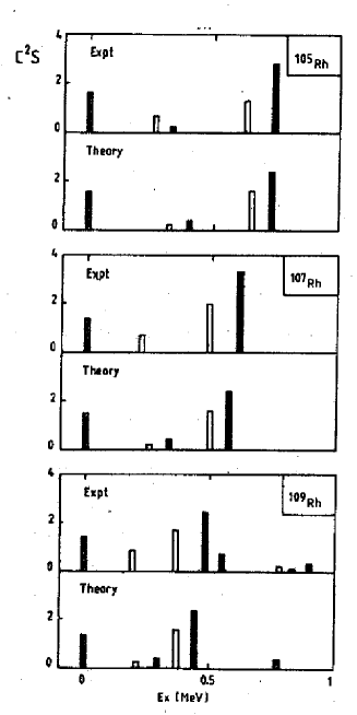
Figure 10: Experimental and calculated spectroscopic factors in Rh isotopes once .

In the same fashion, if we now consider $U(6/12)$ to be the dynamical algebra for the pair of nuclei ¹⁹⁴Pt-¹⁹⁵Pt, it follows that the same $H$ and operators (including in this case the transfer operators that connect states in the different nuclei) should apply to all states. It also follows that no restriction should be imposed on the form of $H$, except that it must be a function of the generators of $U(6/12)$ (the enveloping space associated to it). It should be clear that the concept of supersymmetry does not require the existence of a particular dynamical symmetry. Extending these ideas to the neutron-proton space of IBM-2 we can say that SUSY is equivalent to requiring that a product of the form

$$U_{\nu}(6/\Omega_{\nu})\otimes U_{\pi}(6/\Omega_{\pi})~{},$$ (133)

plays the role of dynamical (super)algebra for a quartet of even-even, even-odd, odd-even and odd-odd nuclei. Having said that, it should be stated that the dynamical supersymmetry has the distinct advantage of immediately suggesting the form of the quartet’s Hamiltonian and operators, while the general statement made above does not provide a general recipe. For some particular cases, however, this can be done in a straightforward way. In reference once , for example, the $U(6/12)$ supersymmetry (without imposing any of the three dynamical IBM symmetries) was successfully tested for the Ru and Rh isotopes. In that case a combination of $U^{BF}(5)$ and $SO^{BF}(6)$ symmetries was shown to give an excellent description of the data, as shown in Figs. 9 and 10.

An immediate consequence of this proposal is that it opens up the possibility of testing SUSY in other nuclear regions, since dynamical symmetries are very scarce and have severely limited the study of nuclear supersymmetry.

4 Summary and Conclusions

In these lecture notes we have discussed different aspects of supersymmetry in nuclear physics. We have attempted to give a general overview of the subject, starting from the fundamental concepts in group theory and Lie algebras, which are the required mathematical framework for this phenomenon.

The recent measurements of the spectroscopic properties of the odd-odd nucleus ¹⁹⁶Au have rekindled the interest in nuclear supersymmetry, as has been discussed in some detail. The available data on the spectroscopy of the quartet of nuclei ¹⁹⁴Pt, ¹⁹⁵Au, ¹⁹⁵Pt and ¹⁹⁶Au can, to a good approximation, be described in terms of the $U(6/4)_{\pi}\otimes U(6/12)_{\nu}$ supersymmetry. However, there is a still another important set of experiments which can further test the predictions of the supersymmetry scheme. These involve transfer reactions between nuclei belonging to the same supermultiplet, in particular between the even-odd (odd-even) and odd-odd members of the supersymmetric quartet. Theoretically, these transfers are described by the supersymmetric generators which change a boson into a fermion, or vice versa.

We have discussed the example of proton transfer between the SUSY partners: ¹⁹⁴Pt $\rightarrow$ ¹⁹⁵Au and ¹⁹⁵Pt $\rightarrow$ ¹⁹⁶Au. The supersymmetry implies strong correlations for the spectroscopic factors of these two reactions which can be tested experimentally. A similar set of relations can be derived for the one-neutron transfer reactions ¹⁹⁴Pt $\leftrightarrow$ ¹⁹⁵Pt and ¹⁹⁵Au $\leftrightarrow$ ¹⁹⁶Au. Another interesting extension of supersymmetry concerns the recently measured two-nucleon transfer reaction ¹⁹⁴Pt$(\alpha,d)^{196}$Au graw , in which a neutron-proton pair is transferred to the target nucleus. This reaction presents a very sensitive test of the wave functions, since it provides a measure of the correlation within the transferred neutron-proton pair. Whether it is possible to describe this process by a transfer operator that is correlated by SUSY to that of the one-proton and one-neutron transfer reactions is an open question.In these lecture notes we have also argued that n-Susy can in principle be generalized to encompass transitional nuclei, that is, that do not correspond to dynamical symmetries.

Figure 11: Detail of “The School of Athens” (Plato on the left and Aristoteles on the right), by Rafael.

In conclusion, we have reviewed the current status of nuclear supersymmetry and considered diverse extensions that are currently being investigated. We have emphasized the need for further experiments taking advantage of new experimental capabilities tres ; pt195 ; au196 , suggesting that particular attention be paid to one- and two-nucleon transfer reactions between the SUSY partners ¹⁹⁴Pt, ¹⁹⁵Au, ¹⁹⁵Pt and ¹⁹⁶Au, since such experiments provide the most stringent tests of nuclear supersymmetry. It remains to be seen whether the correlations predicted by n-SUSY are indeed verified by new experiments and whether these correlations can be truly extended to mixed-symmetry regions of the nuclear table. If this is the case, nuclear supersymmetry may yet provide a powerful unifying scheme for atomic nuclei, thus becoming a particularly striking example of the combination of the Platonic ideal of symmetry with the down-to-earth Aristotelic ability to recognize complex patterns in Nature.

References

-
(1)
A. Arima and F. Iachello,
Phys. Rev. Lett. 35, 1069 (1975);
F. Iachello and A. Arima, The Interacting Boson Model, (Cambridge University Press, Cambridge, 1987). -
(2)
F. Iachello and O. Scholten,
Phys. Rev. Lett. 43, 679 (1979);
F. Iachello and P. Van Isacker, The Interacting Boson-Fermion Model (Cambridge University Press, Cambridge, 1991). - (3) F. Iachello, Phys. Rev. Lett. 44, 772 (1980).
-
(4)
A.B. Balantekin, I. Bars and F. Iachello,
Phys. Rev. Lett. 47, 19 (1981);
A.B. Balantekin, I. Bars and F. Iachello, Nucl. Phys. A 370, 284 (1981). - (5) A.B. Balantekin, I. Bars, R. Bijker and F. Iachello, Phys. Rev. C 27, 1761 (1983).
- (6) A. Mauthofer, K. Stelzer, J. Gerl, Th.W. Elze, Th. Happ, G. Eckert, T. Faestermann, A. Frank and P. Van Isacker, Phys. Rev. C 34, 1958 (1986).
- (7) R. Bijker, Ph.D. Thesis, University of Groningen (1984).
- (8) D.D. Warner, R.F. Casten and A. Frank, Phys. Lett. B 180, 207 (1986).
- (9) P. Van Isacker, J. Jolie, K. Heyde and A. Frank, Phys. Rev. Lett. 54, 653 (1985).
- (10) A. Frank and P. Van Isacker, Algebraic Methods in Molecular and Nuclear Structure Physics, (Wiley, New York, 1994).
- (11) R. Gilmore, Lie Groups, Lie Algebras, and Some of Their Applications, (Wiley-Interscience, New York, 1974).
- (12) M.E. Rose, Elementary Theory of Angular Momentum, Wiley, New York, 1957.
- (13) B.G. Wybourne, Classical Groups for Physicists, (Wiley-Interscience, New York, 1974).
- (14) H.J. Lipkin, Lie Groups for Pedestrians, (North-Holland, Amsterdam, 1966).
- (15) V.I. Man’ko, in Symmetries in Science V, ed. by B. Gruber, L.C. Biedenharn, and H.D. Doebner, (Plenum, New York, 1991), pp. 453.
- (16) A. Messiah, Quantum Mechanics, (Wiley, New York, 1968).
- (17) O. Castaños, A. Frank, and R. Lopez–Peña, J. Phys. A 23, 5141 (1990).
- (18) W. Heisenberg, Z. Phys. 77, 1 (1932).
- (19) J.P. Elliott and P.G. Dawber, Symmetry in Physics. I. Principles and Simple Applications (Oxford University Press, New York, 1979).
- (20) A. Bohr and B.R. Mottelson, Nuclear Structure. II. Nuclear Deformations (Benjamin, New York, 1975).
- (21) M. Gell-Mann, Phys. Rev. 125, 1067 (1962).
- (22) S. Okubo, Progr. Theor. Phys. 27, 949 (1962).
- (23) M. Gell-Mann and Y. Ne’eman, The Eightfold Way, (Benjamin, New York, 1964).
- (24) J. Wess and B. Zumino, Nucl. Phys. B 70, 39 (1974).
- (25) P. Fayet and S. Ferrara, Phys. Rep. 32, 249 (1977).
- (26) P. van Nieuwenhuizen, Phys. Rep. 68, 189 (1981).
- (27) S. Weinberg, The quantum theory of fields: Supersymmetry (Cambridge University Press, Cambridge, 2000).
- (28) I. Bars, in Introduction to Supersymmetry in Particle and Nuclear Physics, ed. by O. Castaños, A. Frank, and L. Urrutia, (Plenum, New York, 1983), pp 107.
- (29) A. Metz, J. Jolie, G. Graw, R. Hertenberger, J. Gröger, C. Günther, N. Warr and Y. Eisermann, Phys. Rev. Lett. 83, 1542 (1999).
- (30) A. Kostelecky and D.K. Campbell, Eds., Supersymmetry in Physics (North Holland, Amsterdam, 1984).
- (31) A. Metz, Y. Eisermann, A. Gollwitzer, R. Hertenberger, B.D. Valnion, G. Graw and J. Jolie, Phys. Rev. C 61, 064313 (2000).
- (32) J. Gröger, J. Jolie, R. Krücken, C.W. Beausang, M. Caprio, R.F. Casten, J. Cederkall, J.R. Cooper, F. Corminboeuf, L. Genilloud, G. Graw, C. Günther, M. de Huu, A.I. Levon, A. Metz, J.R. Novak, N. Warr and T. Wendel, Phys. Rev. C 62, 064304 (2000).
- (33) R. Bijker, J. Barea and A. Frank, preprint (2004), submitted to J. Phys. A.
- (34) A. Frank, P. Van Isacker and D.D. Warner, Phys. Lett. B 197, 474 (1987).
- (35) J. Barea, Ph.D. Thesis (2002).
- (36) H.-F. Wirth and G. Graw, private communication.
- (37) J.P. Elliott, Proc. Roy. Soc. A 245, 128 (1958); Proc. Roy. Soc. A 245, 562 (1958).
- (38) F. Iachello and S. Kuyucak, Ann. Phys. (N.Y.) 136, 19 (1981).
-
(39)
J.A. Cizewski, R.F. Casten, G.J. Smith, M.L. Stelts, W.R. Kane,
H.G. Börner and W.F. Davidson,
Phys. Rev. Lett. 40, 167 (1978);
A. Arima and F. Iachello, Phys. Rev. Lett. 40, 385 (1978). -
(40)
H.Z. Sun, A. Frank and P. Van Isacker,
Phys. Rev. C 27, 2430 (1983);
H.Z. Sun, A. Frank and P. Van Isacker, Ann. Phys. (N.Y.) 157, 183 (1984). - (41) A. Mauthofer, K. Stelzer, Th.W. Elze, Th. Happ, J. Gerl, A. Frank and P. Van Isacker, Phys. Rev. C 39, 1111 (1989).
- (42) J. Jolie, U. Mayerhofer, T. von Egidy, H. Hiller, J. Klora, H. Lindner and H. Trieb, Phys. Rev. C 43, R16 (1991).
- (43) G. Rotbard, G. Berrier, M. Vergnes, S. Fortier, J. Kalifa, J.M. Maison, L. Rosier, J. Vernotte, P. Van Isacker and J. Jolie, Phys. Rev. C 47, 1921 (1993).
- (44) O. Scholten, Prog. Part. Nucl. Phys. 14, 189 (1985).
- (45) R. Bijker and F. Iachello, Ann. Phys. (N.Y.) 161, 360 (1985).
- (46) J. Barea, R. Bijker, A. Frank and G. Loyola, Phys. Rev. C 64, 064313 (2001).
- (47) M.L. Munger and R.J. Peterson, Nucl. Phys. A 303, 199 (1978).
- (48) Y. Yamazaki and R.K. Sheline, Phys. Rev. C 14, 531 (1976).
- (49) H.-F. Wirth, S. Christen, Y. Eisermann, A. Gollwitzer, G. Graw, R. Hertenberger, J. Jolie, A. Metz, O. Möller, D. Tonev and B.D. Valnion, preprint (2004).
- (50) J. Barea, C.E. Alonso and J.M. Arias, Phys. Rev. C 65, 034328 (2002).
- (51) I. Talmi, Simple Models for Complex Nuclei, (Harwood, 1993).
- (52) P. Navrátil alnd J. Dobes, Phys. Rev. C 37, 2126 (1988).