Entrainment coefficient and effective mass for conduction neutrons in neutron star crust : simple microscopic models

Abstract. In the inner crust of a neutron star, at densities above the “drip” threshold, unbound “conduction” neutrons can move freely past through the ionic lattice formed by the nuclei. The relative current density ${\color[rgb]{0,0.6,0.0}n}^{i}={\color[rgb]{0,0.6,0.0}n}\bar{\color[rgb]{0.4,0,0.2}v}^{i}$ of such conduction neutrons will be related to the corresponding mean particle momentum ${\color[rgb]{1,0,0}p}_{i}$ by a proportionality relation of the form ${\color[rgb]{0,0.6,0.0}n}^{i}={{\color[rgb]{0.4,0,0.2}{\cal K}}}{\color[rgb]{1,0,0}p}^{i}$ in terms of a physically well defined mobility coefficient ${{\color[rgb]{0.4,0,0.2}{\cal K}}}$ whose value in this context has not been calculated before. Using methods from ordinary solid state and nuclear physics, a simple quantum mechanical treatment based on the independent particle approximation, is used here to formulate ${{\color[rgb]{0.4,0,0.2}{\cal K}}}$ as the phase space integral of the relevant group velocity over the neutron Fermi surface. The result can be described as an “entrainment” that changes the ordinary neutron mass ${\color[rgb]{1,0,0}m}$ to a macroscopic effective mass per neutron that will be given – subject to adoption of a convention specifying the precise number density ${\color[rgb]{0,0.6,0.0}n}$ of the neutrons that are considered to be “free” – by ${\color[rgb]{1,0,0}m}_{\star}={\color[rgb]{0,0.6,0.0}n}/{{\color[rgb]{0.4,0,0.2}{\cal K}}}\,.$ The numerical evaluation of the mobility coefficient is carried out for nuclear configurations of the “lasagna” and “spaghetti” type that may be relevant at the base of the crust. Extrapolation to the middle layers of the inner crust leads to the unexpected prediction that ${\color[rgb]{1,0,0}m}_{\star}$ will become very large compared with ${\color[rgb]{1,0,0}m}\,.$

1 Introduction

The main purpose of this article is to show how a mean field treatment of neutron star crust matter can be used to address the previously unsolved problem of evaluating a quantity, namely the relevant neutron mobility coefficient ${\color[rgb]{0.4,0,0.2}{\cal K}}$ , that is essential for the astrophysical applications that will be described in a separate article [1]. In terms of the relevant number density ${\color[rgb]{0,0.6,0.0}n}$ of effectively unbound neutrons, this coefficient determines a corresponding effective mass ${\color[rgb]{1,0,0}m}_{\star}={\color[rgb]{0,0.6,0.0}n}/{\color[rgb]{0.4,0,0.2}{\cal K}}$ that characterises their average motion on a macroscopic scale (meaning one that is large compared with the spacing between nuclei) and that we therefore refer to as the macro mass, to distinguish it from the microscopic effective mass, ${\color[rgb]{1,0,0}m^{{}_{\oplus}}}$ say, characterising the dynamics of the neutrons on subnuclear scales. Whereas ${\color[rgb]{1,0,0}m^{{}_{\oplus}}}$ is well known to be typically rather smaller than the ordinary neutron mass ${\color[rgb]{1,0,0}m}$ , we reach the previously unexpected conclusion that there is likely to be a strong “entrainment” effect whereby the macro mass ${\color[rgb]{1,0,0}m}_{\star}$ will typically become large, and in some layers extremely large, compared with ${\color[rgb]{1,0,0}m}$ .

A secondary purpose of this article is to draw the attention of nuclear theorists to the potentialities of the almost entirely unexplored branch of theoretical astrophysical nuclear physics that needs to be developed for this and many other purposes. The only relevant work of which we are aware so far is that of Oyamatsu and Yamada  [2], who appear to be the only ones to have taken proper account of the neutron scattering by the nuclei inside the inner crust by the use of appropriate Bloch type periodicity conditions of the kind commonly employed for the treatment of electrons in ordinary terrestrial solid state physics. Their treatment however was restricted to a simple one dimensional model.

Under the conditions of ordinary terrestrial solid state physics, and even at the much higher densities characterising the matter in a white dwarf star, long range electric forces keep the nuclei so far apart that, in so far as the much stronger but short range nuclear interactions are concerned, each individual nucleus can be treated separately as if it were isolated. Until quite recently [2], such a separate treatment of individual nuclei (considered as if isolated each in its own cell - with Wigner Seitz type boundary conditions) has been used in nearly all quantum mechanical calculations on neutron star crust matter since the pioneer work of Negele and Vautherin [3]. That kind of approximation is fully justifiable in the outer crust , where the densities are not too much greater than those found in a white dwarf. However such a treatment can no longer be considered entirely satisfactory in the inner crust, meaning the part with density above the “neutron drip” threshold at about 10¹¹ g/cm³, where there are unconfined neutrons that travel between neighbouring nuclei, which thereby cease to be effectively isolated from one another.

While desirable for accuracy throughout the inner crust, a proper collective rather than individual treatment of the nuclei becomes not just desirable but absolutely essential for treating the problem with which Oyamatsu and Yamada  [2] [4] were concerned, namely that of the nuclear matter inside neutron star crust. Such a treatment is also essential for treating the problem with which the present work is concerned, namely that of stationary but non static configurations in which a neutron current flows relative to the lattice formed by the nuclei, something that obviously can not be discussed in the usual approach that treats the nuclei as if they were isolated in individual (e.g. Wigner Seitz type) boxes.

The flow of neutrons is treated here as a perturbation of a zero temperature ground state characterised just by the location of the relevant Fermi surface in momentum space. We thereby obtain provisional rough estimates of the relevant mobility coefficient which suggest that (unlike what occurs in the fluid core and on a microscopic scale) the macro mass ${\color[rgb]{1,0,0}m}_{\star}$ that effectively characterises the neutron motion on a macroscopic scale can become very large compared with the ordinary neutron mass ${\color[rgb]{1,0,0}m}$ , particularly in the middle part of the conducting layer, for which three dimensional numerical results will be presented in a follow up article [6]. The present article deals more specifically with simplified rod and plate type models that are relevant near the crust core interface, where the mass enhancement will be less extreme.

Bulgac, Magierski and Heenen have recently pointed out the importance of shell effects induced by unbound neutrons in neutron star crust by evaluating the Casimir energy for neutron matter in the presence of inhomogeneities from a semiclassical approach and more recently by performing a Skyrme Hartree-Fock calculation with ordinary periodic boundary conditions (see [7, 8] and references therein). However this kind of boundary conditions does not properly account for Bragg scattering of dripped neutrons and is only a particular case of the more general Bloch type boundary conditions.

In the absence of any previous quantum mechanical calculation whereby nuclei on a crystal lattice are treated collectively (apart from the 1D calculation previously mentionned [2]), even at the simplest level of approximation, we shall adopt the simple model suggested by Oyamatsu and Yamada, supplemented with Bloch type boundary conditions, in order to estimate the effective neutron mass ${\color[rgb]{1,0,0}m}_{\star}\,.$ This model treats the neutrons as independent fermions subject to an effective potential. We wish to draw the attention of nuclear theorists to the problem of including Bloch boundary conditions in more sophisticated approximation schemes as a challenge for future work.

In the mean time, experience with the analogous problem of electron transport in ordinary solid state physics suggests that the results obtained from the Oyamatsu Yamada type treatment used here should not be too bad as a first approximation. Further encouragement comes from our own recent attempt to take up the challenge of allowing for coupling by an appropriate adaptation of the standard BCS pairing theory on which the prediction of neutron superfluidity (in the relevant low to moderate temperature range) is based: the upshot [9] is that (although it is essential for the inhibition of resistivity) as far as the “entrainment” phenomenon is concerned the effect of the ensuing pairing “gap” will not be very large nor very difficult to calculate.

2 Microscopic description of conduction neutrons in the inner crust

2.1 Single-particle Schrödinger equation

The basic principle of the conductivity model we wish to adapt from ordinary solid state theory to the context of a neutron star crust is that the “conduction band”, and perhaps also some of the highest “confined” levels, can be analysed within the independent particle approximation, in terms of energy eigenstates for a single particle described by a Bloch type wave function ${\color[rgb]{0.4,0,0.2}\varphi}$ , satisfying the Bloch periodic boundary conditions as discussed below. In the rest frame of the crust, with respect to which the system will be assumed to be in stationary equilibrium, the single particle wave function will be taken to be governed by a Hamiltonian operator ${\color[rgb]{1,0,0}{\cal H}}$ that is given by

$$\color[rgb]{0,0,0}{\color[rgb]{1,0,0}{\cal H}}=-{\color[rgb]{1,0,0}\hbar}^{2}\nabla_{i}\,\frac{\gamma^{ij}}{2{\color[rgb]{1,0,0}m^{{}_{\oplus}}}}\,\nabla_{j}+{\color[rgb]{1,0,0}V}\,,$$ (2.1)

where $\gamma^{ij}$ is just the space metric, while ${\color[rgb]{1,0,0}V}$ is the single particle potential, and ${\color[rgb]{1,0,0}m^{{}_{\oplus}}}$ is the relevant local effective mass parameter.

The potential ${\color[rgb]{1,0,0}V}$ and the effective mass ${\color[rgb]{1,0,0}m^{{}_{\oplus}}}$ will be periodic in the case of a regular crystalline solid lattice, though not for a fluid configuration such as will be relevant at higher temperatures. The value of the effective potential ${\color[rgb]{1,0,0}V}$ (and the associated deviation of the effective mass ${\color[rgb]{1,0,0}m^{{}_{\oplus}}}$ from ${\color[rgb]{1,0,0}m}$ ) is supposed to allow not just for the attraction of the confined protons in the nuclei but also for the mean effect of the other fermions, which are electrons in the familiar solid state applications, but neutrons in the context under consideration here.

2.2 Boundary conditions

The preceding considerations apply even to disordered (glass like or liquid) configurations, but in order to proceede we shall now restrict our attention to cases for which the nuclei are assumed to be fixed and locally distributed in a regular crystal lattice configuration, in which an elementary cell consists of a parallelopiped of volume ${{\color[rgb]{0.3,0.0,0.8}{\cal V}}}_{\rm cell}$ say spanned by a triad of basis vectors ${\bf{\color[rgb]{0.3,0.0,0.8}{e}}}_{\color[rgb]{0.3,0.0,0.8}{\it a}}$ labelled by an index with values ${\color[rgb]{0.3,0.0,0.8}{\it a}}=$ 1, 2, 3, so that the system is invariant with respect to translations generated by vectors of the form

$$\color[rgb]{0,0,0}{\color[rgb]{0,0,0}{\bf T}}={\color[rgb]{0,0,0}{\ell}}^{\color[rgb]{0.3,0.0,0.8}{\it a}}{\bf{\color[rgb]{0.3,0.0,0.8}{e}}}_{\color[rgb]{0.3,0.0,0.8}{\it a}}$$ (2.2)

for integer values of the coefficients ${\color[rgb]{0,0,0}{\ell}}^{\color[rgb]{0.3,0.0,0.8}{\it a}}$ (in the following summation over repeated indices is assumed). This so called adiabatic or Born-Oppenheimer approximation is justified by the large difference between the neutron and nucleus masses, since typically each nucleus contains several hundred nucleons [10].

It follows directly from the well-known Floquet-Bloch theorem [11] that the single particle wave function has to satisfy the following boundary conditions

$$\color[rgb]{0,0,0}{\color[rgb]{0.4,0,0.2}\varphi}_{\bf{\color[rgb]{0,0.6,0.0}k}}\{{\bf r}+{\bf{\color[rgb]{0,0,0}{\bf T}}}\}={\rm e}^{{\rm i}\,{\bf{\color[rgb]{0,0.6,0.0}k}}\cdot{\bf{\color[rgb]{0,0,0}{\bf T}}}}{\color[rgb]{0.4,0,0.2}\varphi}_{\bf{\color[rgb]{0,0.6,0.0}k}}\{{\bf r}\}.$$ (2.3)

where $\bf{\color[rgb]{0,0.6,0.0}k}$ is the Bloch momentum covector.

It will therefore suffice to solve the Schrödinger equation just inside a single elementary cell. Instead of using a primitive cell of parallelopiped, it is convenient for many purposes to work instead with the Wigner-Seitz (W-S) cell defined as the set of points that are closer to a given lattice node than to any other. Such a cell exhibits the full symmetry of the lattice. Its shape is determined by the crystal structure, a polyhedron in general, for instance a cube in a simple cubic lattice. This exactly defined W-S cell should not be confused with the widely employed eponymous “W-S approximation” [12] which consists in replacing this cell by a sphere (or more generally any convenient cell that simplifies the analysis).

The Bloch momentum $\bf{\color[rgb]{0,0.6,0.0}k}$ takes values inside the first Brillouin zone (B-Z), which is the W-S cell of the reciprocal lattice whose nodes are located at ${\color[rgb]{0,0.6,0.0}{\bf K}}={\color[rgb]{0,0.6,0.0}{\ell}}_{\color[rgb]{0.3,0.0,0.8}{\it a}}{\bf{\color[rgb]{0,0,0}{l}}}^{{\color[rgb]{0.3,0.0,0.8}{\it a}}}$ for integer values of the coefficients ${\color[rgb]{0,0.6,0.0}{\ell}}_{\color[rgb]{0.3,0.0,0.8}{\it a}}$ where the dual basis vectors ${\bf{\color[rgb]{0,0,0}{l}}}^{{\color[rgb]{0.3,0.0,0.8}{\it a}}}$ are defined by the following scalar products

$$\color[rgb]{0,0,0}{\bf{\color[rgb]{0,0,0}{l}}^{{\color[rgb]{0.3,0.0,0.8}{\it a}}}\cdot{\color[rgb]{0.3,0.0,0.8}{e}}_{{\color[rgb]{0.3,0.0,0.8}{\it b}}}}=2\pi\delta^{\color[rgb]{0.3,0.0,0.8}{\it a}}_{\color[rgb]{0.3,0.0,0.8}{\it b}}\,,$$ (2.4)

the $2\pi$ normalization factor being introduced for convenience.

It must be emphasized that the single particle wave function will have to satisfy the relation (2.3) between two opposite faces of the cell. This means in particular that the Schrödinger equation has to be solved for each wave vector $\bf{\color[rgb]{0,0.6,0.0}k}$ inside the first B-Z. The ordinary periodic boundary conditions on the cell, which have been recently applied by Magierski and Heenen [8], are thus only a restricted subset of solutions, namely those with ${\bf{\color[rgb]{0,0.6,0.0}k}}=0.$

For each momentum $\bf{\color[rgb]{0,0.6,0.0}k}$ , there exists only a discrete set of energy eigenvalues satisfying the Bloch boundary conditions. The single particle energy spectrum is therefore a collection of sheets in momentum space, each sheet usually being referred as a band (labelled by the principal quantum number).

3 Microscopic dynamics in mean field of lattice

3.1 From microscopic to macroscopic observables

The linearisation involved in the neglect of direct two body or many body interactions in such a mean field treatment excludes allowance for higher order effects such as the pairing responsible for a superfluid energy gap, but as discussed in a separate article [9], this limitation should not matter too much for the evaluation of the basic equation of state of the fluid, since the main effect of superfluidity is not to modify the equation of motion but just to restrain the class of the admissible solutions (by allowing only those that are irrotational).

The main limitation on the use of such a linearisation is that it makes sense only for configurations that do not differ too much from the static reference configuration on which the estimation of the effective potential energy function ${\color[rgb]{1,0,0}V}$ is based.

3.2 Fermi surface in ground state configuration

The zero temperature configuration is obtained by minimising an energy density ${\color[rgb]{1,0,0}U}$ subject to the constraint of a given value of the neutron density ${\color[rgb]{0,0.6,0.0}n}_{\rm n}\,,$ defined by

$$\color[rgb]{0,0,0}{\color[rgb]{0,0.6,0.0}n}_{\rm n}=\int{{\rm d}^{3}{\color[rgb]{0,0.6,0.0}k}\over(2\pi)^{3}}\,.$$ (3.1)

The energy density is expressible in terms of the single particle energies (in this work, we shall use braces instead of ordinary brackets for functional dependence, in order to avoid possibly confusion with simple multiplication)

$$\color[rgb]{0,0,0}{\color[rgb]{1,0,0}{\cal H}}{\color[rgb]{0.4,0,0.2}\varphi}_{\bf{\color[rgb]{0,0.6,0.0}k}}={{\color[rgb]{1,0,0}{\cal E}}}\{{\bf{\color[rgb]{0,0.6,0.0}k}}\}{\color[rgb]{0.4,0,0.2}\varphi}_{\bf{\color[rgb]{0,0.6,0.0}k}}\,,$$ (3.2)

by an expression of the form

$$\color[rgb]{0,0,0}{\color[rgb]{1,0,0}U}={\color[rgb]{1,0,0}U}\{0\}+\int{{\color[rgb]{1,0,0}{\cal E}}}\{{\bf{\color[rgb]{0,0.6,0.0}k}}\}{{\rm d}^{3}{\color[rgb]{0,0.6,0.0}k}\over(2\pi)^{3}}\,,$$ (3.3)

where, as a standard postulate, the contribution ${\color[rgb]{1,0,0}U}\{0\}$ is ignored in the minimisation procedure. This means that all single particle states of energy up to but not beyond some particular Fermi level, ${\color[rgb]{1,0,0}\mu}$ say, are occupied. This Fermi energy specifies the “Fermi surface”, namely the locus, ${\color[rgb]{0,0.6,0.0}S}_{{}_{\rm F}}$ say, in momentum space, where

$$\color[rgb]{0,0,0}{{\color[rgb]{1,0,0}{\cal E}}}\{{\bf{\color[rgb]{0,0.6,0.0}k}}\}={\color[rgb]{1,0,0}\mu}\,.$$ (3.4)

It must be emphasised that the Fermi surface will in general consist of disconnected pieces unlike the homogenous case in which the Fermi surface is simply a sphere. From the property that ${\color[rgb]{1,0,0}{\cal E}}\{{\bf{\color[rgb]{0,0.6,0.0}k}}\}={\color[rgb]{1,0,0}{\cal E}}\{-{\bf{\color[rgb]{0,0.6,0.0}k}}\},$ the ground state is thus completely symmetric in the sense that its total momentum density $\int{\rm d}^{3}{\color[rgb]{0,0.6,0.0}k}\,{\color[rgb]{0,0.6,0.0}k}^{i}$ vanishes. This is a generalized version of Unsöld theorem [13] according to which the all electron wave function of a closed shell atom is spherically symmetric.

3.3 Minimal conducting configurations

Our main concern in the present analysis is with current carrying configurations, as characterised by some given value of the physically well defined number current density with components ${\color[rgb]{0,0.6,0.0}n}^{i}$ given by

$$\color[rgb]{0,0,0}{\color[rgb]{0,0.6,0.0}n}^{i}=\int{\color[rgb]{0.4,0,0.2}v}^{i}{{\rm d}^{3}{\color[rgb]{0,0.6,0.0}k}\over(2\pi)^{3}}$$ (3.5)

in which the transport velocity ${\color[rgb]{0.4,0,0.2}v}^{i}$ is given by the formula

$$\color[rgb]{0,0,0}{\color[rgb]{0.4,0,0.2}v}^{i}=\frac{1}{{\color[rgb]{1,0,0}\hbar}}\frac{\partial{\color[rgb]{1,0,0}{\cal E}}}{\partial k_{i}}\,.$$ (3.6)

The kind of current carrying configurations that will presumably be relevant in the low temperature limit will be those for which the energy density ${\color[rgb]{1,0,0}U}$ is minimised for a given value of the neutron density ${\color[rgb]{0,0.6,0.0}n}_{\rm n}$ subject to the further constraint that the number current density also has the prescribed value ${\color[rgb]{0,0.6,0.0}n}^{i}.$ It is evident that this constrained minimisation condition requires that the occupied states should consist just of those subject to an inequality of the form

$$\color[rgb]{0,0,0}{{\color[rgb]{1,0,0}{\cal E}}}\leq{\color[rgb]{1,0,0}\mu}+{\color[rgb]{1,0,0}p}_{i}\,{\color[rgb]{0.4,0,0.2}v}^{i}\,,$$ (3.7)

for some fixed covector whose constant components ${\color[rgb]{1,0,0}p}_{i}$ have been introduced as Lagrange multipliers. The phase space volume specified in this way will have a boundary characterised by the condition

$$\color[rgb]{0,0,0}{{\color[rgb]{1,0,0}{\cal E}}}={\color[rgb]{1,0,0}\mu}+{\color[rgb]{1,0,0}p}_{i}\,{\color[rgb]{0.4,0,0.2}v}^{i}\,,$$ (3.8)

which specifies a modified Fermi surface, ${\color[rgb]{0,0.6,0.0}S}$ say. The constraint of having a finite current breaks the symmetry and will thus necessarily lead to a new ground state with a non vanishing total momentum density vector $\int{\rm d}^{3}{\color[rgb]{0,0.6,0.0}k}\,{\color[rgb]{0,0.6,0.0}k}^{i}\neq 0$ .

3.4 The uniform displacement of the Fermi surface

To justify the use of a Schrödinger type Hamiltonian ${\color[rgb]{1,0,0}{\cal H}}$ involving an effective potential of the same form as in the zero current case, we need to assume that (as will presumably be the case in the relevant context of pulsar glitches) the current density ${\color[rgb]{0,0.6,0.0}n}^{i}$ is small enough to be treated by linear perturbation theory. This means that the Lagrange multiplier ${\color[rgb]{1,0,0}p}_{i}$ should itself be considered just as a first order perturbation, having zero value ${\color[rgb]{1,0,0}p}_{i}=0$ in the static unperturbed configuration, and ${\color[rgb]{1,0,0}p}_{i}=\delta{\color[rgb]{1,0,0}p}_{i}$ in the perturbed current carrying configuration. For a given (unchanged) value of the chemical potential ${\color[rgb]{1,0,0}\mu}$ , the difference between the new value (3.8)  and the old value (3.4)  of the Fermi energy level ${\color[rgb]{1,0,0}{\cal E}}$ will be given to first order by $\delta{\color[rgb]{1,0,0}{\cal E}}=\delta({\color[rgb]{1,0,0}p}_{i}\,{\color[rgb]{0.4,0,0.2}v}^{i})$ $={\color[rgb]{0.4,0,0.2}v}^{i}\,\delta{\color[rgb]{1,0,0}p}_{i}$ and thus in terms of the perturbed value of ${\color[rgb]{1,0,0}p}_{i}$ simply by

$$\color[rgb]{0,0,0}\delta{\color[rgb]{1,0,0}{\cal E}}={\color[rgb]{1,0,0}p}_{i}\,{\color[rgb]{0.4,0,0.2}v}^{i}\,.$$ (3.9)

This change in energy can be interpreted as being attributable to a phase space displacement $\delta{\color[rgb]{0,0.6,0.0}k}_{i}.$ Since this change will be given, according to (3.6)  , by

$$\color[rgb]{0,0,0}\delta{{\color[rgb]{1,0,0}{\cal E}}}={\color[rgb]{1,0,0}\hbar}{\color[rgb]{0.4,0,0.2}v}^{i}\delta{\color[rgb]{0,0.6,0.0}k}_{i}\,,$$ (3.10)

it can be seen that the simplest possibility is to take the displacement to have the uniform value given just by

$$\color[rgb]{0,0,0}{\color[rgb]{1,0,0}\hbar}\delta{\color[rgb]{0,0.6,0.0}k}_{i}={\color[rgb]{1,0,0}p}_{i}\,,$$ (3.11)

as illustrated on figure 1.

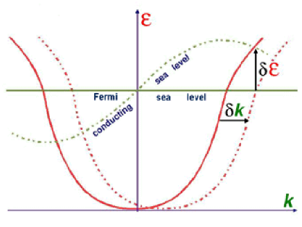
Figure 1: Sketch of energy against wave number, showing uniform displacement attributable to current.

3.5 Relation between current and momentum

The relation (3.11)  means that (in the infinitesimal limit) the Lagrange multipliers ${\color[rgb]{1,0,0}p}_{i}$ can be physically interpreted simply as components of a uniform pseudo momentum displacement of the occupied phase space region, and of its “Fermi surface” boundary.

The effect of this displacement on the Fermi surface element ${\rm d}{\color[rgb]{0,0.6,0.0}S}_{{}_{\rm F}}{{}^{i}}$ as given – in terms of the corresponding surface measure element, ${\rm d}{\color[rgb]{0,0.6,0.0}S}_{{}_{\rm F}}$ – by

$$\color[rgb]{0,0,0}{\rm d}{\color[rgb]{0,0.6,0.0}S}_{{}_{\rm F}}{{}^{i}}=({\color[rgb]{0.4,0,0.2}v}^{i}/{\color[rgb]{0.4,0,0.2}v}){\rm d}{\color[rgb]{0,0.6,0.0}S}_{{}_{\rm F}}\,,$$ (3.12)

will be to sweep out an infinitesimal phase space volume element given by

$$\color[rgb]{0,0,0}{\color[rgb]{1,0,0}\hbar}{\rm d}^{3}{\color[rgb]{0,0.6,0.0}k}={\color[rgb]{1,0,0}p}_{i}\,{\rm d}{\color[rgb]{0,0.6,0.0}S}_{{}_{\rm F}}^{\,i}\,.$$ (3.13)

It follows that, for the integral over the occupied region of any phase space function $f\,,$ the difference between the value for the displaced (conducting) configuration and the value for the non conducting reference configuration will be given (to linear order) by the formula

$$\color[rgb]{0,0,0}{\color[rgb]{1,0,0}\hbar}\,\delta\!\int\!f\,{\rm d}^{3}{\color[rgb]{0,0.6,0.0}k}={\color[rgb]{1,0,0}p}_{i}\oint_{{}_{\rm F}}\!f\,{\rm d}{\color[rgb]{0,0.6,0.0}S}_{{}_{\rm F}}^{\,i}\,,$$ (3.14)

in which it is to be understood that the integral on the right is taken over the entire Fermi surface.

We have already pointed out that the energy function ${\color[rgb]{1,0,0}{\cal E}}$ will be symmetric with respect to the origin, hence it follows that the Fermi surface element ${\rm d}{\color[rgb]{0,0.6,0.0}S}_{{}_{\rm F}}^{\,i}$ will be antisymmetric about the origin so that its unweighted integral $\oint_{{}_{\rm F}}{\rm d}{\color[rgb]{0,0.6,0.0}S}_{{}_{\rm F}}^{\,i}$ will self cancel to give zero. We can thus see from (3.14)  that for any phase space function $f$ that is symmetric about the origin the corresponding integral will be unaffected by the displacement, i.e. we shall get $\delta\int f\,{\rm d}^{3}{\color[rgb]{0,0.6,0.0}k}=0$ . This contrasts with the case of an antisymmetric function, for which it is the unperturbed integral that will vanish, i.e. we shall have $\int f\,{\rm d}^{3}{\color[rgb]{0,0.6,0.0}k}=0$ in the static reference configuration, so that the corresponding value for the conducting configuration will be given by $\int f\,{\rm d}^{3}{\color[rgb]{0,0.6,0.0}k}=\delta\int f\,{\rm d}^{3}{\color[rgb]{0,0.6,0.0}k}$ .

The antisymmetric case is illustrated by the application with which this work is principally concerned, namely the current density ${\color[rgb]{0,0.6,0.0}n}^{i}$ given by (3.5)  . Since we have ${\color[rgb]{0,0.6,0.0}n}^{i}=0$ in the reference configuration characterised by ${\color[rgb]{1,0,0}p}_{i}=0$ , we shall have ${\color[rgb]{0,0.6,0.0}n}^{i}=\delta{\color[rgb]{0,0.6,0.0}n}^{i}$ in the conducting configuration characterised by ${\color[rgb]{1,0,0}p}_{i}=\delta{\color[rgb]{1,0,0}p}_{i}$ . Thus by substituting ${\color[rgb]{0.4,0,0.2}v}^{i}$ for $f$ in (3.14)  we see that in the linearised limit the current will be related to the pseudo momentum displacement ${\color[rgb]{1,0,0}p}_{i}$ by a relation of the form

$$\color[rgb]{0,0,0}{\color[rgb]{0,0.6,0.0}n}^{i}={{\color[rgb]{0.4,0,0.2}{\cal K}}}^{ij}{\color[rgb]{1,0,0}p}_{j}\,,$$ (3.15)

in which the symmetric tensor ${\color[rgb]{0.4,0,0.2}{\cal K}}^{ij}$ is given as an integral over the Fermi surface by

$$\color[rgb]{0,0,0}{{\color[rgb]{0.4,0,0.2}{\cal K}}}^{ij}={1\over(2\pi)^{3}{\color[rgb]{1,0,0}\hbar}}\oint_{{}_{\rm F}}\!{{\color[rgb]{0.4,0,0.2}v}^{i}{\color[rgb]{0.4,0,0.2}v}^{j}\over{\color[rgb]{0.4,0,0.2}v}}\,dS_{{}_{\rm F}}\,.$$ (3.16)

Before continuing, it is to be remarked that this tensor ${\color[rgb]{0.4,0,0.2}{\cal K}}^{ij}$ is interpretable as being proportional to the zero temperature limit of the electric conductivity tensor ${\color[rgb]{1,0,0}\sigma}^{ij},$ defined in the usual way by ${\color[rgb]{1,0,0}j}^{i}={\color[rgb]{1,0,0}\sigma}^{ij}{\color[rgb]{0,0,0}\rm E}_{j}$ where ${\color[rgb]{0,0,0}\rm E}_{j}$ is the relevant electric field and ${\color[rgb]{1,0,0}j}^{i}$ the electric current density, by a relation of the form ${\color[rgb]{1,0,0}\sigma}^{ij}=\tau{\color[rgb]{1,0,0}e}^{2}{{\color[rgb]{0.4,0,0.2}{\cal K}}}^{ij},$ where $\tau$ is the relevant relaxation time and ${\color[rgb]{1,0,0}e}$ the electric charge per particle.

In a entirely disordered (liquid or glass like) state the form of the energy function ${\color[rgb]{1,0,0}{\cal E}}$ and the consequent location in phase space of the Fermi surface will be difficult to evaluate theoretically, but there will be the partially compensating simplification that the result will automatically be isotropic. In the mathematically simpler case of a cubic crystalline lattice that is expected [14] to occur in a neutron star crust, this tensor ${\color[rgb]{0.4,0,0.2}{\cal K}}^{ij}$ will have the isotropic form

$$\color[rgb]{0,0,0}{{\color[rgb]{0.4,0,0.2}{\cal K}}}^{ij}={{\color[rgb]{0.4,0,0.2}{\cal K}}}\gamma^{ij}\,,$$ (3.17)

in which the scalar coefficient will evidently be given by

$$\color[rgb]{0,0,0}{{\color[rgb]{0.4,0,0.2}{\cal K}}}={{}_{1}\over{}^{3}}\gamma_{ij}{{\color[rgb]{0.4,0,0.2}{\cal K}}}^{ij}\,.$$ (3.18)

However that may be, it can be seen from (3.16)  that the scalar coefficient ${\color[rgb]{0.4,0,0.2}{\cal K}}$ will be given by a Fermi surface integral of the simple form

$$\color[rgb]{0,0,0}{{\color[rgb]{0.4,0,0.2}{\cal K}}}={1\over 3(2\pi)^{3}{\color[rgb]{1,0,0}\hbar}}\oint_{{}_{\rm F}}\!{\color[rgb]{0.4,0,0.2}v}\,{\rm d}{\color[rgb]{0,0.6,0.0}S}_{{}_{\rm F}}\,.$$ (3.19)

In terms of this integral, the relation between current and momentum will be given by

$$\color[rgb]{0,0,0}{\color[rgb]{0,0.6,0.0}n}^{i}={{\color[rgb]{0.4,0,0.2}{\cal K}}}\gamma^{ij}{\color[rgb]{1,0,0}p}_{j}\,.$$ (3.20)

3.6 The (cut-off dependent) concept of the effective mean mass

In order to relate the formula (3.19)  to expressions used elsewhere in the literature, it is to be noted that we can introduce a mean velocity vector $\bar{v}^{i}$ and a conduction neutron density ${\color[rgb]{0,0.6,0.0}n}$ such that the current density can be expressed by

$$\color[rgb]{0,0,0}{\color[rgb]{0,0.6,0.0}n}^{i}={\color[rgb]{0,0.6,0.0}n}\bar{v}^{i}\,.$$ (3.21)

Subject to the isotropy condition (3.17)  , the (pseudo) momentum covector ${\color[rgb]{1,0,0}p}_{i}$ will be expressible in terms of the corresponding covector $\bar{v}_{i}=\gamma_{ij}\bar{v}^{j}$ in the simple form

$$\color[rgb]{0,0,0}{\color[rgb]{1,0,0}p}_{i}={\color[rgb]{1,0,0}m}_{\star}\bar{v}_{i}\,,$$ (3.22)

in which the effective mean particle mass ${\color[rgb]{1,0,0}m}_{\star}$ – which we refer to as the “macro mass” in order to distinguish it from the locally effective “‘micro mass” ${\color[rgb]{1,0,0}m^{{}_{\oplus}}}$ – is defined in terms of the integral (3.19)  by the relation

$$\color[rgb]{0,0,0}{1\over{\color[rgb]{1,0,0}m}_{\star}}={{{\color[rgb]{0.4,0,0.2}{\cal K}}}\over{\color[rgb]{0,0.6,0.0}n}}\,.$$ (3.23)

It is however to be remarked that whereas the specification of quantities such as ${\color[rgb]{1,0,0}p}_{i}$ and ${\color[rgb]{0.4,0,0.2}{\cal K}}$ is physically unambiguous, the specification of the effective mass ${\color[rgb]{1,0,0}m}_{\star}$ , like that of the mean transport velocity $\bar{v}^{i}$ , depends on how many “conduction states” are counted in the definition of the number density ${\color[rgb]{0,0.6,0.0}n}\,,$ and how many are left aside as dynamically inert “confined” states.

In the application to a neutron star crust, the situation is somewhat simpler than is usual in ordinary solid state physics because the relevant single particle Hamiltonian (2.1)  will usually involve an effective potential function ${\color[rgb]{1,0,0}V}$ that tends rapidly [15] towards an almost exactly uniform value outside the ionic nuclei to which all the protons and some of the neutrons are effectively confined. It should be noticed that the single particle wave function of bound states will be vanishingly small at the W-S cell boundary and therefore those states will not be sensitive to the Bloch phase shift. The resulting single particle energies will thus be nearly independent of the Bloch momentum which means that the associated group velocities will be very small. The single particle energy spectrum can therefore be decomposed into a subset consisting of such confined states, and a remainder that will realistically be describable as “conduction” states. The separation between those two different subsets is not entirely sharp (borderline states are commonly refered to as valence states in ordinary solid state physics) and one has to rely on a more or less arbitrary convention.

In most layers of a neutron star crust, the most convenient possibility is usually to take the uniform value of ${\color[rgb]{1,0,0}V}$ outside nuclei, which can be taken as the energy origin, to specify a corresponding energy range ${{\color[rgb]{1,0,0}{\cal E}}}>0$ characterising “conduction” states. This specification may however be ambiguous in the bottom layers of the inner crust where nuclei are very close to each other. In order to deal with such cases, we shall adopt the convention, which agrees with the previous one when nuclei are very far apart, that conduction states are defined as states whose energy is larger than the maximum value of the potential.

It is to be remarked that in the uniform limit whereby the periodic potential ${\color[rgb]{1,0,0}V}$ and the local effective mass ${\color[rgb]{1,0,0}m^{{}_{\oplus}}}$ are simply constants, the resulting Fermi surface is a sphere and the evaluation of the mobility scalar is straightforward. In this case, the associated macro mass is just equal to the micro mass ${\color[rgb]{1,0,0}m}_{\star}={\color[rgb]{1,0,0}m^{{}_{\oplus}}}$ provided all neutron states are counted as conduction states.

4 Quantitative estimates of the mobility tensor

4.1 Bottom layer of the inner crust

We shall focus for simplicity on the bottom of the inner crust near saturation density of the order of $10^{14}$ g/cm³ where the transition to homogeneous fluid neutron matter takes place, to evaluate the mobility scalar and the effective mass. In this region the crystal lattice is not expected to substantially alter the transport properties such as the mobility tensor. The aim of the following sections is not to provide astrophysically important information but rather to give some insight that may be valuable in the more general cases that will be dealt with in future work. Near the base of the crust, the nuclei are so strongly deformed by their neighbours that they may adopt non spherical shapes [16], sometimes idealised by 1D or 2D configurations such as slabs and rods respectively, which greatly simplifies the analysis. These “exotic” crust phases are illustrated on figure 2 taken from the work of Oyamatsu [4].

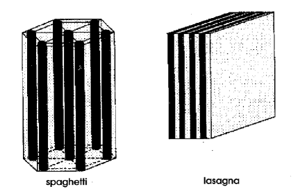
Figure 2: Nuclear configurations for hexagonal spaghetti (rod) and lasagna (slab) lattices. Black - nuclear matter; grey - neutron gas. From [4], with kind permission of the author.

In views of the exploratory character of the present work, we shall use a simple model for the single particle equation. In particular, we shall drop the condition of strict self-consistency, and shall use a mean field model based on the work of Oyamatsu [4, 2]. He calculated the structure of the ground state of the inner neutron star crust using a phenomenological energy-density functional, fitted on the first hand to the smoothed nuclear masses and charged radii of laboratory nuclei on the $\beta$ stability line and on the other hand adjusted on the equation of state of pure neutron matter from the variational calculations of Friedman and Pandharipande [5] using two body as well as three body nucleon-nucleon interactions. He further investigated with Yamada the importance of shell effects with a single particle Schrödinger equation in the W-S approximation [2] (the reader is refered to those two papers for the details).

Unlike the calculations carried out by these authors, we shall apply the 1D or 2D Bloch type boundary conditions and we shall not make any approximations about the shape of the W-S cells which partition the crystal. The 3D configurations require specific numerical techniques and will be discussed in a separate work [6]. For consistency, the lattice parameters (whose values are found in [4]) will be defined so that the volume of the exact W-S cell is equal to the volume of the approximate cell. Within a W-S cell, we approximate the single particle potential ${\color[rgb]{1,0,0}V}$ by the potential ${\color[rgb]{1,0,0}U}$ of Oyamatsu and Yamada [2]. A zeroth order approximation ${\color[rgb]{1,0,0}U}_{0}$ of the potential is obtained by differentiation of the potential part of an energy density functional $v\{{\color[rgb]{0,0.6,0.0}n}_{\rm n},{\color[rgb]{0,0.6,0.0}n}_{\color[rgb]{0.6,0.4,0.0}\rm p}\}$ so that

$$\color[rgb]{0,0,0}{\color[rgb]{1,0,0}U}_{0}=\frac{\partial v}{\partial{\color[rgb]{0,0.6,0.0}n}_{\rm n}}.$$ (4.1)

Specifically we shall use the parameter set of model I of this paper. Then, the effect of the finite range of the nucleon-nucleon interaction is taken into account by using the folding of the potential ${\color[rgb]{1,0,0}U}_{0}$ with a gaussian smearing function of width $\kappa.$ This potential is supplemented with a spin-orbit coupling term, which is parametrized as a functional of the density gradients. The gaussian width and the parameters of the spin-orbit potential are adjusted so as to reproduce the correct sequence of single particle energy levels of ²⁰⁸Pb. The potential ${\color[rgb]{1,0,0}U}$ thus obtained varies only near the nuclear surface. Therefore, close to the W-S cell boundary ${\color[rgb]{1,0,0}U}$ is constant. This enables us to express the periodic potential ${\color[rgb]{1,0,0}V}$ acting on a neutron moving in an infinite lattice of nuclei as

$$\color[rgb]{0,0,0}{\color[rgb]{1,0,0}V}\{{\bf r}\}=\sum_{{\color[rgb]{0,0,0}{\bf T}}}{\color[rgb]{1,0,0}U}\{{\bf r}-{{\color[rgb]{0,0,0}{\bf T}}}\}~{},$$ (4.2)

where the sum goes over all nuclei occupying the lattice sites, i.e. ${\bf{\color[rgb]{0,0,0}{\bf T}}}={\color[rgb]{0,0,0}{\ell}}^{\color[rgb]{0.3,0.0,0.8}{\it a}}{\bf{\color[rgb]{0.3,0.0,0.8}{e}}}_{\color[rgb]{0.3,0.0,0.8}{\it a}}$ , where ${\color[rgb]{0,0,0}{\ell}}^{\color[rgb]{0.3,0.0,0.8}{\it a}}$ are integers. The potential ${\color[rgb]{1,0,0}V}\{{\bf r}\}$ thus possesses all the symmetries of the crystal lattice. We neglect small changes in ${\color[rgb]{1,0,0}U}$ due to passing from a single W-S cell to an infinite lattice. The energy origin is taken as the value of the potential ${\color[rgb]{1,0,0}V}$ outside nuclei. Following Oyamatsu and Yamada [2] we do not include momentum dependent terms in the single particle potential. Consequently the microscopic effective neutron mass in this model is just equal to the bare neutron mass ${\color[rgb]{1,0,0}m^{{}_{\oplus}}}={\color[rgb]{1,0,0}m}\,.$ We have ignored the spin-orbit coupling since it is found to be about one order of magnitude smaller than the central potential [2].

The single-particle Schrödinger equation is solved here by the Rayleigh-Ritz variational approach whereby the expectation value of the Hamiltonian is minimized subject to a normalization condition. The single particle wave function is expanded into plane waves defined by

$$\color[rgb]{0,0,0}{\color[rgb]{0.4,0,0.2}\varphi}_{\bf{\color[rgb]{0,0.6,0.0}k}}\{{\bf r}\}=\frac{1}{\sqrt{{\color[rgb]{0.3,0.0,0.8}{\cal V}}_{\rm cell}}}\sum_{{\color[rgb]{0,0.6,0.0}{\bf K}}}\tilde{{\color[rgb]{0.4,0,0.2}\varphi}}_{\bf{\color[rgb]{0,0.6,0.0}k}}\{{{\color[rgb]{0,0.6,0.0}{\bf K}}}\}\,{\rm e}^{{\rm i}\,({\bf{\color[rgb]{0,0.6,0.0}k}}+{\color[rgb]{0,0.6,0.0}{\bf K}})\cdot{\bf r}}\,,$$ (4.3)

with the normalization

$$\color[rgb]{0,0,0}\sum_{{\color[rgb]{0,0.6,0.0}{\bf K}}}|\tilde{{\color[rgb]{0.4,0,0.2}\varphi}}_{\bf{\color[rgb]{0,0.6,0.0}k}}({{\color[rgb]{0,0.6,0.0}{\bf K}}})|^{2}=1\,.$$ (4.4)

This expansion into plane waves is actually exact, it merely makes more apparent the periodicity. The approximation lies in the fact that the summation needs to be truncated for practical calculations at some cut off energy ${\color[rgb]{1,0,0}{\cal E}}_{\rm cutoff}$ (which thus makes this method adequate only for slowly varying potentials as in the present case), i.e. so as to include all reciprocal lattice vectors satisfying

$$\color[rgb]{0,0,0}\frac{{\color[rgb]{1,0,0}\hbar}^{2}({\bf{\color[rgb]{0,0.6,0.0}k}+{\color[rgb]{0,0.6,0.0}{\bf K}}})^{2}}{2{\color[rgb]{1,0,0}m}}<{\color[rgb]{1,0,0}{\cal E}}_{\rm cutoff}\,.$$ (4.5)

The group velocity is found according to the Hellmann-Feynman theorem [17] to be equal to

$$\color[rgb]{0,0,0}{\bf{\color[rgb]{0.4,0,0.2}v}}=\frac{{\color[rgb]{1,0,0}\hbar}{\bf{\color[rgb]{0,0.6,0.0}k}}}{{\color[rgb]{1,0,0}m}}+\sum_{\color[rgb]{0,0.6,0.0}{\bf K}}\frac{{\color[rgb]{1,0,0}\hbar}{\color[rgb]{0,0.6,0.0}{\bf K}}}{{\color[rgb]{1,0,0}m}}|\tilde{{\color[rgb]{0.4,0,0.2}\varphi}}_{\bf{\color[rgb]{0,0.6,0.0}k}}({{\color[rgb]{0,0.6,0.0}{\bf K}}})|^{2}\,.$$ (4.6)

This last equation shows that deviations from the homogeneous case arise from the spreading of the Bloch wave packet (4.3).

For each total neutron density ${\color[rgb]{0,0.6,0.0}n}_{{\rm n}}$ , the Fermi energy ${\color[rgb]{1,0,0}\mu}$ is determined as an integral over the first B-Z by

$$\color[rgb]{0,0,0}{\color[rgb]{0,0.6,0.0}n}_{{\rm n}}=\frac{2}{(2\pi)^{3}}\sum_{{\color[rgb]{0.4,0,0.2}\alpha}}\int_{{}_{\rm BZ}}{\rm d}^{3}{\color[rgb]{0,0.6,0.0}k}\,\vartheta\{{\color[rgb]{1,0,0}\mu}-{{\color[rgb]{1,0,0}{\cal E}}}_{\color[rgb]{0.4,0,0.2}\alpha}\}\,,$$ (4.7)

where we have introduced the Heaviside unit step distribution defined by $\vartheta\{x\}=1$ if $x>0$ and zero otherwise (the factor of 2 is to account for the spin degeneracy). The conduction neutron density is defined by the occupied single particle states whose energy is positive, i.e. ${{\color[rgb]{1,0,0}{\cal E}}}_{{\color[rgb]{0.4,0,0.2}\alpha}}>0$ , namely

$$\color[rgb]{0,0,0}{\color[rgb]{0,0.6,0.0}n}=\frac{2}{(2\pi)^{3}}\sum_{{\color[rgb]{0.4,0,0.2}\alpha}}\int_{{}_{\rm BZ}}{\rm d}^{3}{\color[rgb]{0,0.6,0.0}k}\,\vartheta\{{\color[rgb]{1,0,0}\mu}-{{\color[rgb]{1,0,0}{\cal E}}}_{\color[rgb]{0.4,0,0.2}\alpha}\}\vartheta\{{{\color[rgb]{1,0,0}{\cal E}}}_{\color[rgb]{0.4,0,0.2}\alpha}\}\,.$$ (4.8)

It will be instructive to compare the Fermi surface area with that of a non interacting neutron gas of density ${\color[rgb]{0,0.6,0.0}n}_{{\rm n}}$ , which is given by

$$\color[rgb]{0,0,0}{{\color[rgb]{0,0.6,0.0}S}}_{\rm gas}=4\pi(3\pi^{2}{\color[rgb]{0,0.6,0.0}n}_{{\rm n}})^{2/3}\,.$$ (4.9)

4.2 “Lasagna” phase

In this model, the slab shaped nuclei or “lasagna” are parallel to each other and equally spaced by a distance $a$ . Hence the single particle potential ${\color[rgb]{1,0,0}V}$ is periodic along one direction only, say the $z$ axis, and takes a constant value in the other two dimensions. The neutron band structure with a square well potential (whose analytic solution was found a long time ago by Kronig and Penney [18, 19]) was the only case discussed by Oyamatsu and Yamada [2].

The single particle wavefunction can be factored in the form

$$\color[rgb]{0,0,0}{\color[rgb]{0.4,0,0.2}\varphi}_{\bf{\color[rgb]{0,0.6,0.0}k}}\{{\bf r}\}=\phi_{{\color[rgb]{0,0.6,0.0}k}_{z}}\{z\}{\rm e}^{{\rm i}\,({\color[rgb]{0,0.6,0.0}k}_{x}x+{\color[rgb]{0,0.6,0.0}k}_{y}y)}\,,$$ (4.10)

in which the reduced wave funtion $\phi_{{\color[rgb]{0,0.6,0.0}k}_{z}}$ is the solution of a one dimensional equation of the form

$$\color[rgb]{0,0,0}\frac{-{\color[rgb]{1,0,0}\hbar}^{2}}{2{\color[rgb]{1,0,0}m}}\frac{d^{2}\phi_{{\color[rgb]{0,0.6,0.0}k}_{z}}}{dz^{2}}+{\color[rgb]{1,0,0}V}\{z\}\phi_{{\color[rgb]{0,0.6,0.0}k}_{z}}\{z\}={\color[rgb]{1,0,0}{\varepsilon}}\{{\color[rgb]{0,0.6,0.0}k}_{z}\}\phi_{{\color[rgb]{0,0.6,0.0}k}_{z}}\{z\}\,,$$ (4.11)

satisfying the boundary conditions

$$\color[rgb]{0,0,0}\phi_{{\color[rgb]{0,0.6,0.0}k}_{z}}\{z+a\}=e^{{\rm i}\,{\color[rgb]{0,0.6,0.0}k}_{z}a}\phi_{{\color[rgb]{0,0.6,0.0}k}_{z}}\{z\}\,.$$ (4.12)

The first B-Z is defined by the set of Bloch wave vectors such that $-\pi/a\leq{\color[rgb]{0,0.6,0.0}k}_{z}\leq\pi/a.$ The B-Z in this peculiar case has an infinite extent as a result of the continuous translational invariance along planes parallel to the “lasagna”. The single particle energy is thus given by an expression of the form

$$\color[rgb]{0,0,0}{{\color[rgb]{1,0,0}{\cal E}}}_{{\color[rgb]{0.4,0,0.2}\alpha}}\{{\bf{\color[rgb]{0,0.6,0.0}k}}\}=\frac{{\color[rgb]{1,0,0}\hbar}^{2}({\color[rgb]{0,0.6,0.0}k}_{x}^{2}+{\color[rgb]{0,0.6,0.0}k}_{y}^{2})}{2{\color[rgb]{1,0,0}m}}+{\color[rgb]{1,0,0}{\varepsilon}}_{{\color[rgb]{0.4,0,0.2}\alpha}}\{{\color[rgb]{0,0.6,0.0}k}_{z}\},$$ (4.13)

where ${\color[rgb]{0.4,0,0.2}\alpha}$ is a band index. It follows that the neutron group velocity components parallel to the slabs coincide with the group velocity of a non interacting neutron gas while only the component perpendicular to the slabs is affected. It can be shown from group theoretical arguments, that this component of the group velocity must vanish at the Brillouin zone edge [20], i.e. at ${\color[rgb]{0,0.6,0.0}k}_{z}=\pm\pi/a$ . More generally whenever the Bloch wave vector lies on a symmetry plane, the group velocity component normal to the plane vanishes . It can also be shown that the energy bands do not cross [20](nevertheless bands may touch “accidentally” for some specific choice of potential, for instance a constant one).

The total neutron density is given by

$$\color[rgb]{0,0,0}{\color[rgb]{0,0.6,0.0}n}_{{\rm n}}=\frac{{\color[rgb]{1,0,0}m}}{\pi^{2}{\color[rgb]{1,0,0}\hbar}^{2}}\sum_{{\color[rgb]{0.4,0,0.2}\alpha}}\int_{0}^{\pi/a}{\rm d}{\color[rgb]{0,0.6,0.0}k}_{z}\bigl{(}{\color[rgb]{1,0,0}\mu}-{\color[rgb]{1,0,0}{\varepsilon}}_{{\color[rgb]{0.4,0,0.2}\alpha}}\bigr{)}\vartheta\{{\color[rgb]{1,0,0}\mu}-{\color[rgb]{1,0,0}{\varepsilon}}_{{\color[rgb]{0.4,0,0.2}\alpha}}\}\,.$$ (4.14)

The mobility along the “lasagna” planes coincides with that of the uniform neutron gas with the same total neutron density:

$$\color[rgb]{0,0,0}{{\color[rgb]{0.4,0,0.2}{\cal K}}}^{\parallel}={{\color[rgb]{0.4,0,0.2}{\cal K}}}^{xx}={{\color[rgb]{0.4,0,0.2}{\cal K}}}^{yy}=\frac{{\color[rgb]{0,0.6,0.0}n}_{{\rm n}}}{{\color[rgb]{1,0,0}m}}\,.$$ (4.15)

The mobility in directions perpendicular to the “lasagna” may however differ from that of the non interacting neutron gas:

$$\color[rgb]{0,0,0}{{\color[rgb]{0.4,0,0.2}{\cal K}}}^{\perp}={{\color[rgb]{0.4,0,0.2}{\cal K}}}^{zz}=\frac{1}{4\pi^{3}{\color[rgb]{1,0,0}\hbar}}\sum_{{\color[rgb]{0.4,0,0.2}\alpha}}\int\frac{({\color[rgb]{0.4,0,0.2}v}^{z})^{2}}{{\color[rgb]{0.4,0,0.2}v}}{\rm d}{\color[rgb]{0,0.6,0.0}S}_{{}_{\rm F}}^{({\color[rgb]{0.4,0,0.2}\alpha})}=\frac{{\color[rgb]{1,0,0}m}}{\pi^{2}{\color[rgb]{1,0,0}\hbar}^{4}}\sum_{{\color[rgb]{0.4,0,0.2}\alpha}}\int_{0}^{\pi/a}\biggl{(}\frac{d{\color[rgb]{1,0,0}{\varepsilon}}_{{\color[rgb]{0.4,0,0.2}\alpha}}}{d{\color[rgb]{0,0.6,0.0}k}_{z}}\biggr{)}^{2}\vartheta\{{\color[rgb]{1,0,0}\mu}-{\color[rgb]{1,0,0}{\varepsilon}}_{{\color[rgb]{0.4,0,0.2}\alpha}}\}{\rm d}{\color[rgb]{0,0.6,0.0}k}_{z}\,.$$ (4.16)

Since the “lasagna” configuration is strongly anisotropic, it is more appropriate to define a transverse effective macro mass by

$$\color[rgb]{0,0,0}{\color[rgb]{1,0,0}m}_{\star}^{\perp}\equiv\frac{{\color[rgb]{0,0.6,0.0}n}}{{{\color[rgb]{0.4,0,0.2}{\cal K}}}^{\perp}}.$$ (4.17)

The conduction neutron density is expressible as

$$\color[rgb]{0,0,0}{\color[rgb]{0,0.6,0.0}n}={\color[rgb]{0,0.6,0.0}n}_{{\rm n}}+\frac{4}{(2\pi)^{3}}\sum_{{\color[rgb]{0.4,0,0.2}\alpha}}\int_{0}^{\pi/a}\pi\frac{2{\color[rgb]{1,0,0}m}{\color[rgb]{1,0,0}{\varepsilon}}_{\color[rgb]{0.4,0,0.2}\alpha}}{{\color[rgb]{1,0,0}\hbar}^{2}}\vartheta\{{\color[rgb]{1,0,0}\mu}-{\color[rgb]{1,0,0}{\varepsilon}}_{{\color[rgb]{0.4,0,0.2}\alpha}}\}\vartheta\{-{\color[rgb]{1,0,0}{\varepsilon}}_{\color[rgb]{0.4,0,0.2}\alpha}\}{\rm d}{\color[rgb]{0,0.6,0.0}k}_{z}\,.$$ (4.18)

4.3 “Spaghetti” phase

In the spaghetti model, the crystal is composed of cylinder shaped nuclei arranged on a two dimensional lattice (the nuclear “spaghetti” are assumed to be parallel to each other along say the z axis). Since the single particle potential around one isolated nucleus only depends on the distance to the rod like nucleus, the corresponding contribution to the crystal potential does not depend on $z$ hence the wave function can be factored as

$$\color[rgb]{0,0,0}{\color[rgb]{0.4,0,0.2}\varphi}_{\bf{\color[rgb]{0,0.6,0.0}k}}\{{\bf r}\}=\phi_{{\color[rgb]{0,0.6,0.0}k}_{x},{\color[rgb]{0,0.6,0.0}k}_{y}}\{x,y\}{\rm e}^{{\rm i}\,{\color[rgb]{0,0.6,0.0}k}_{z}z}\,.$$ (4.19)

The two dimensional wave function obeys a Schrödinger equation of the form

$$\color[rgb]{0,0,0}-\frac{{\color[rgb]{1,0,0}\hbar}^{2}}{2{\color[rgb]{1,0,0}m}}\biggl{(}\frac{\partial^{2}}{\partial x^{2}}+\frac{\partial^{2}}{\partial y^{2}}\biggr{)}\phi_{{\color[rgb]{0,0.6,0.0}k}_{x},{\color[rgb]{0,0.6,0.0}k}_{y}}\{x,y\}+{\color[rgb]{1,0,0}V}\{x,y\}\phi_{{\color[rgb]{0,0.6,0.0}k}_{x},{\color[rgb]{0,0.6,0.0}k}_{y}}\{x,y\}={\color[rgb]{1,0,0}{\varepsilon}}\{{\color[rgb]{0,0.6,0.0}k}_{x},{\color[rgb]{0,0.6,0.0}k}_{y}\}\phi_{{\color[rgb]{0,0.6,0.0}k}_{x},{\color[rgb]{0,0.6,0.0}k}_{y}}\{x,y\}\,.$$ (4.20)

The energy is thus decomposible as

$$\color[rgb]{0,0,0}{{\color[rgb]{1,0,0}{\cal E}}}_{{\color[rgb]{0.4,0,0.2}\alpha}}\{{\bf{\color[rgb]{0,0.6,0.0}k}}\}={\color[rgb]{1,0,0}{\varepsilon}}_{{\color[rgb]{0.4,0,0.2}\alpha}}\{{\color[rgb]{0,0.6,0.0}k}_{x},{\color[rgb]{0,0.6,0.0}k}_{y}\}+\frac{{\color[rgb]{1,0,0}\hbar}^{2}{\color[rgb]{0,0.6,0.0}k}_{z}^{2}}{2{\color[rgb]{1,0,0}m}}\,.$$ (4.21)

The total neutron density is given by

$$\color[rgb]{0,0,0}{\color[rgb]{0,0.6,0.0}n}_{{\rm n}}=\frac{4}{(2\pi)^{3}{\color[rgb]{1,0,0}\hbar}}\sum_{{\color[rgb]{0.4,0,0.2}\alpha}}\int_{{}_{\rm BZ}}\sqrt{2{\color[rgb]{1,0,0}m}({\color[rgb]{1,0,0}\mu}-{\color[rgb]{1,0,0}{\varepsilon}}_{{\color[rgb]{0.4,0,0.2}\alpha}})}\,\vartheta\{{\color[rgb]{1,0,0}\mu}-{\color[rgb]{1,0,0}{\varepsilon}}_{{\color[rgb]{0.4,0,0.2}\alpha}}\}{\rm d}{\color[rgb]{0,0.6,0.0}k}_{x}{\rm d}{\color[rgb]{0,0.6,0.0}k}_{y}\,,$$ (4.22)

in which the factor of two arises from the restriction that ${\color[rgb]{0,0.6,0.0}k}_{z}>0$ and where the integration is carried out over the 2D first B-Z illustrated on figure 4.

It is readily verified that the mobility tensor component along the cylindrical nuclei is merely equal to the mobility component of the non interacting neutron gas:

$$\color[rgb]{0,0,0}{{\color[rgb]{0.4,0,0.2}{\cal K}}}^{\parallel}={{\color[rgb]{0.4,0,0.2}{\cal K}}}^{zz}=\frac{{\color[rgb]{0,0.6,0.0}n}_{{\rm n}}}{{\color[rgb]{1,0,0}m}}\,.$$ (4.23)

The other components perpendicular to the “spaghetti” depend on the neutron-crystal interaction. It is convenient to defined a mean transverse mobility by

$$\color[rgb]{0,0,0}{{\color[rgb]{0.4,0,0.2}{\cal K}}}^{\perp}=\sqrt{\frac{{\color[rgb]{1,0,0}m}}{2}}\frac{2}{(2\pi)^{3}{\color[rgb]{1,0,0}\hbar}^{3}}\sum_{{\color[rgb]{0.4,0,0.2}\alpha}}\int_{{}_{\rm BZ}}\frac{{\rm d}{\color[rgb]{0,0.6,0.0}k}_{x}{\rm d}{\color[rgb]{0,0.6,0.0}k}_{y}}{\sqrt{{\color[rgb]{1,0,0}\mu}-{\color[rgb]{1,0,0}{\varepsilon}}_{{\color[rgb]{0.4,0,0.2}\alpha}}}}\left(\biggl{(}\frac{\partial{\color[rgb]{1,0,0}{\varepsilon}}_{{\color[rgb]{0.4,0,0.2}\alpha}}}{\partial{\color[rgb]{0,0.6,0.0}k}_{x}}\biggr{)}^{2}+\biggl{(}\frac{\partial{\color[rgb]{1,0,0}{\varepsilon}}_{{\color[rgb]{0.4,0,0.2}\alpha}}}{\partial{\color[rgb]{0,0.6,0.0}k}_{y}}\biggr{)}^{2}\right)\,\vartheta\{{\color[rgb]{1,0,0}\mu}-{\color[rgb]{1,0,0}{\varepsilon}}_{{\color[rgb]{0.4,0,0.2}\alpha}}\},$$ (4.24)

since it involves the integral of a completely symmetric function that can thus be factored into one irreducible domain of the first B-Z [21].

The Fermi surface area, the mobility tensor and the density involve integrations over the two dimensional first B-Z of functions weighted by a Fermi distribution. We have followed an idea due to Gilat and Raubenheimer for three dimensional crystals [22], and translated it into the two dimensional case. First of all the zone is decomposed into small identical cells within which the single particle energy is linearly extrapolated from the value of the energy and its gradient at the center of the cell. The integration is then performed analytically inside the cell. The integral is approximated by summing the contribution from each cell (properly weighted whenever the cells overfill the zone). Unlike the case of band crossing, extrapolation fails for band “kissing” where the energy gradient varies rapidly in the cell (see the schematic pictures on Figure 3). This problem becomes more and more acute as the number of bands to be included in the integration is increased. However those induced systematic errors will tend to vanish as the number of microcells is increased. Whereas the integrand could be integrated analytically inside each microcell, we found that it is better to take it as constant. The reason again lies in the band “kissing” problem. The integrand typically depends on the momentum via the single particle energy which is extrapolated. Near a band kissing region, the extrapolation errors in the integrand are integrated which lead to unstable results.

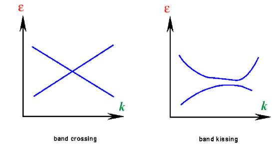
Figure 3: Sketch of energy against wave number for crossing and “kissing” scenarios.

We have considered two lattice types: square and hexagonal crystals (whose reciprocal lattices are also square and hexagonal respectively). The point group $\cal P$ (the set of point symmetries which send the lattice into itself) of the hexagonal lattice is $C_{6v}$ (Schönflies notation [23]) whose order is equal to $|{\cal P}|=12,$ thereby reducing integrations of completely symmetric functions over the entire two dimensional first B-Z to $1/12^{\rm th}$ of the zone. We mention that for this structure the lattice spacing $a$ (shortest distance between any two lattice points) is not equal to the value given by Oyamatsu $a_{{}_{\rm Oy}}$ but is given by

$$\color[rgb]{0,0,0}a=\sqrt{\frac{2}{\sqrt{3}}}\,a_{{}_{\rm Oy}}\,.$$ (4.25)

Likewise, the first B-Z of a square lattice whose point group is $C_{4v}$ (lattice spacing $a=a_{{}_{\rm Oy}}$ ) can be partitionned into $8$ irreducible domains. These considerations are illustrated in Figure 4 with the conventional labelling (first B-Z in red, one irreducible domain in green). The most adequate cell for integrations is thus a rectangle since the irreducible B-Zs are rectangular triangles. The partition of this domain into microcells is thereby straightforward.

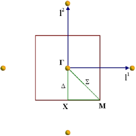
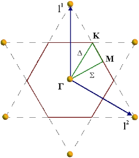
Figure 4: First Brillouin zones and irreducible domains for square and hexagonal variants of spaghetti (rod) lattice.

These two groups, $C_{6v}$ and $C_{4v}$ , contains two dimensional irreducible representations [23] which means that unlike the 1D case, energy bands may cross each other [20]. The neutron band structure along high symmetry lines is shown on Figures 5 and 6 for energies in the vicinity of the Fermi energy and for the lattice spacing $a_{{}_{\rm Oy}}=27.17\,\rm fm\,.$

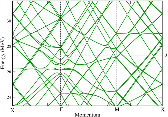
Figure 5: Neutron band structure around the Fermi energy ${\color[rgb]{1,0,0}\mu}$ , along directions shown on figure 4 for square variant of spaghetti (rod) lattice ( $a_{{}_{\rm Oy}}=27.17$ fm).

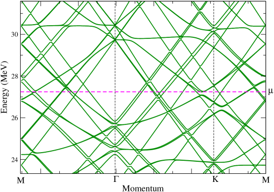
Figure 6: Neutron band structure around the Fermi energy ${\color[rgb]{1,0,0}\mu}$ , along directions shown on figure 4 for hexagonal variant of spaghetti (rod) lattice with $a_{{}_{\rm Oy}}=27.17\,\rm fm\,.$

The conduction neutron density is equal to

$$\color[rgb]{0,0,0}{\color[rgb]{0,0.6,0.0}n}={\color[rgb]{0,0.6,0.0}n}_{{\rm n}}-\frac{4}{(2\pi)^{3}{\color[rgb]{1,0,0}\hbar}}\sum_{{\color[rgb]{0.4,0,0.2}\alpha}}\int_{\rm BZ}\sqrt{-2{\color[rgb]{1,0,0}m}{\color[rgb]{1,0,0}{\varepsilon}}_{{\color[rgb]{0.4,0,0.2}\alpha}}}\,\vartheta\{{\color[rgb]{1,0,0}\mu}-{\color[rgb]{1,0,0}{\varepsilon}}_{{\color[rgb]{0.4,0,0.2}\alpha}}\}\vartheta\{-{\color[rgb]{1,0,0}{\varepsilon}}_{\color[rgb]{0.4,0,0.2}\alpha}\}{\rm d}{\color[rgb]{0,0.6,0.0}k}_{x}{\rm d}{\color[rgb]{0,0.6,0.0}k}_{y}\,.$$ (4.26)

The transverse effective mass is defined by

$$\color[rgb]{0,0,0}{\color[rgb]{1,0,0}m}_{\star}^{\perp}\equiv\frac{{\color[rgb]{0,0.6,0.0}n}}{{{\color[rgb]{0.4,0,0.2}{\cal K}}}^{\perp}}.$$ (4.27)

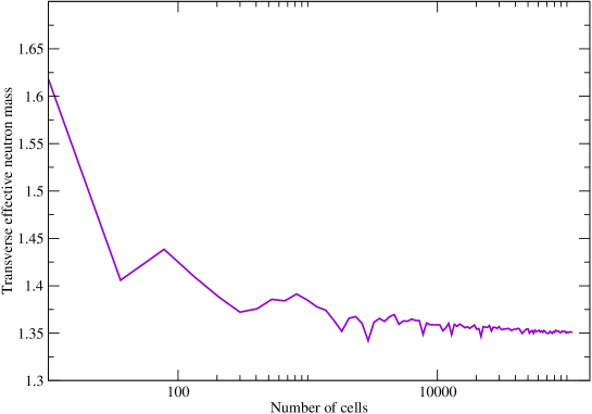
Figure 7: Convergence of computed effective mass ${\color[rgb]{1,0,0}m}_{\star}^{\perp}/{\color[rgb]{1,0,0}m}$ as a function of cell number for an hexagonal lattice with $a_{{}_{\rm Oy}}=27.17\,\rm fm\,.$

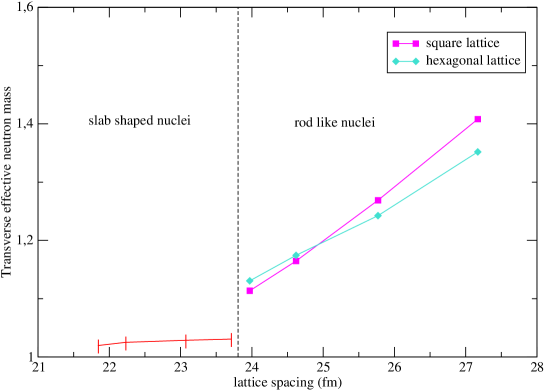
Figure 8: Effective mass of conduction neutrons ${\color[rgb]{1,0,0}m}_{\star}^{\perp}/{\color[rgb]{1,0,0}m}$ as a function of lattice spacing ( $a_{{}_{\rm Oy}}$ ) below and above phase transition from lasagna (slab) regime to spaghetti (rod) regime.

The convergence of the integration scheme based on a decomposition into rectangular cells is illustrated on figure 7 for the hexagonal lattice with the lattice spacing $a_{{}_{\rm Oy}}=27.17\,\rm fm\,.$ The convergence is much faster for the density than for the other quantities due to the absence of the singular square root integrand.

5 Discussion

The results concerning the macroscopic effective neutron mass are illustrated on figure 8 and numerical values can be found in the appendix. The macroscopic effective neutron mass appears to be increased compared to the ordinary neutron mass. The figure also shows that this renormalisation of the neutron mass is mostly significant at low densities and becomes negligible at higher densities where nuclei nearly merge into a uniform mixture. The deviations of the effective neutron mass from the bare one can be understood in terms of modifications of the Fermi surface from a sphere. In particular, as a result of the opening of band gaps the Fermi surface is not smooth but contains many holes as schematically illustrated on figure 9. Since the enclosed Fermi volume only depends on the density, this means that the Fermi surface area for a given density is reduced as compared to the corresponding sphere as shown on figure 10 (see the appendix for the numerical values). In the case for which the Fermi volume is equal to the volume of the first Brillouin zone, the Fermi sphere can be distorted and torn such that the resulting surface area simply vanishes while the volume remains finite. Such a situation occurs in ordinary electric insulators.

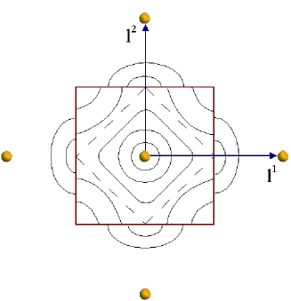
Figure 9: Example of energy contours in extended Brillouin zone for square lattice. For sufficiently small Fermi energies the contours are approximately circular as in the free particle case, while at higher energies, the contours consist of disconnected pieces.

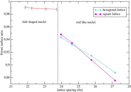
Figure 10: Fermi surface area for neutrons ${{\color[rgb]{0,0.6,0.0}S}}_{{}_{\rm F}}/{{\color[rgb]{0,0.6,0.0}S}}_{\rm gas}$ as a function of lattice spacing ( $a_{{}_{\rm Oy}}$ ) below and above phase transition from lasagna (slab) regime to spaghetti (rod) regime.

In the present work we have neglected the spin-orbit coupling which is a small perturbation in the density region we considered. Taking into account such term would raise some degeneracies. The most dramatic change concerns some regions in momentum space around which unperturbed bands are crossing. The breaking of the spin symmetry will entail that such configuration may be turned into band “kissing” (see figure 3) which means that the group velocity will be strongly reduced around those momenta. This means that the resulting mobility would be lower than the one we have found. Besides, since the conduction neutron density is rather unsensitive to such change, it would not be much affected and therefore the effective neutron mass would be slightly larger than the one calculated here.

6 Conclusion

The scattering of dripped neutrons by the nuclei in the inner crust leads on a macroscopic scale to a modification of the neutron mass ${\color[rgb]{1,0,0}m}_{\star}$ , which can be expressed via a well defined mobility scalar ${\color[rgb]{0.4,0,0.2}{\cal K}}$ by ${\color[rgb]{1,0,0}m}_{\star}={\color[rgb]{0,0.6,0.0}n}/{\color[rgb]{0.4,0,0.2}{\cal K}}$ in which ${\color[rgb]{0,0.6,0.0}n}$ is the (arbitrary) density of such unbound neutrons, and ${\color[rgb]{0.4,0,0.2}{\cal K}}$ is found to be expressible as an integral of the group velocity ${\color[rgb]{0.4,0,0.2}v}^{i}$ over the corresponding Fermi surface. This effective macro mass should not be confused with the effective micro mass, relevant for subnuclear scales, which is usually found to be smaller than the ordinary neutron mass.

Bragg scattering of dripped neutrons is taken into account here by applying Bloch type boundary conditions, which are well known in solid state physics but have been barely used in this nuclear context. We have computed numerical values of this mobility scalar in the bottom layers of the inner crust near the crust-core interface, for simple models in the “pasta” layers: equally spaced slab shaped nuclei (“lasagna”) and rod like nuclei on either a square or an hexagonal 2D lattice (“spaghetti”). The (anisotropic) entrainment effect is small at such densities since the system is nearly homogeneous. It appears that the mobility scalar tends to be systematically reduced compared to the homogeneous expression and the farther from homogeneity, the smaller is the mobility scalar. The resulting effective mass ${\color[rgb]{1,0,0}m}_{\star}$ is found to be larger than the bare neutron mass. This results can be interpreted as a macroscopic manifestation of the modifications in the shape of the Fermi surface. Notably as one goes from the homogeneous outer core to the crust, the spherical neutron Fermi surface gets distorted and even torn and pierced.

The main reason is that the neutron Bragg scattering by crustal nuclei leads to the opening of energy band gaps. A specific feature of those exotic phases is that the mobility scalar is bounded, ${\color[rgb]{0.4,0,0.2}{\cal K}}\geq 2{\color[rgb]{0,0.6,0.0}n}_{{\rm n}}/3{\color[rgb]{1,0,0}m}$ for the “lasagna” phase and ${\color[rgb]{0.4,0,0.2}{\cal K}}\geq{\color[rgb]{0,0.6,0.0}n}_{{\rm n}}/3{\color[rgb]{1,0,0}m}$ for the “spaghetti” phase due to the fact that the neutrons are still free to move in one or two dimensions, respectively. There is no such bound for three dimensional crystals, for which smaller mobility scalars (larger effective masses) may be expected.

From these considerations, we can infer that the mobility scalar ${\color[rgb]{0.4,0,0.2}{\cal K}}$ will increase with the density, starting from zero in the outer crust below the neutron drip threshold where all neutrons are confined, since ${\color[rgb]{0.4,0,0.2}v}^{i}=0$ for all states, to its largest possible value in the homogeneous neutron star mantle. At low densities near neutron drip, where the conduction neutron density is negligible compared to the total neutron density, ${\color[rgb]{0,0.6,0.0}n}\ll{\color[rgb]{0,0.6,0.0}n}_{{\rm n}}\,,$ the crystal potential ${\color[rgb]{1,0,0}V}$ is quite large but the fraction of the cell occupied by the nuclei is small so that dripped neutrons propagate essentially freely. Consequently we may expect to get ${\color[rgb]{0.4,0,0.2}{\cal K}}\simeq{\color[rgb]{0,0.6,0.0}n}/{\color[rgb]{1,0,0}m}$ and ${\color[rgb]{1,0,0}m}_{\star}\simeq{\color[rgb]{1,0,0}m}$ (on the understanding that, as discussed in Subsection 3.6, a conduction state is defined so as to have an associated group velocity that differs significantly from zero). On the other hand, at very high densities where nuclei nearly merge, the potential is much weaker and smoothly varying and we shall have ${\color[rgb]{0,0.6,0.0}n}\simeq{\color[rgb]{0,0.6,0.0}n}_{{\rm n}}\,,$ so we expect to find ${\color[rgb]{1,0,0}m}_{\star}\simeq{\color[rgb]{1,0,0}m}\,.$

In other words the mean effective mass ${\color[rgb]{1,0,0}m}_{\star}$ is expected to be close to the ordinary mass ${\color[rgb]{1,0,0}m}$ at the top (above neutron drip density where neutrons start to leak out of nuclei) and bottom (where nuclei merge into a uniform mixture of neutrons, protons and electrons at density about $1/3$ or $2/3$ the nuclear saturation density ${\color[rgb]{0,0.6,0.0}n}_{\rm sat}\simeq 0.16\,{\rm fm}^{-3}$ [24]) of the inner crust, but may reach a much larger value (with astrophysically interesting consequences) in the intermediate layers. This indicates that the unbound neutron band effects (that are effectively neglected in the commonly used W-S approximation) could have important consequences as concerns the equilibrium neutron star crust structure and composition.

The exploratory character of the present work, justifies the simplicity of the single particle model we used. In a more realistic, Hartree-Fock calculation, the single particle potential and effective micro mass should have to be determined self-consistently. The potential may contain momentum dependent terms, as with effective nucleon-nucleon interactions of the Skyrme type, which leads to space varying effective neutron masses ${\color[rgb]{1,0,0}m}^{{}_{\oplus}}\{{\bf r}\}$ which are typically smaller than the bare neutron mass. However the general arguments we developed, relying on the shape of the Fermi surface, suggest that the qualitative results of our calculations, namely the enhancement of the macroscopic effective mass ${\color[rgb]{1,0,0}m}_{\star}$ will remain valid in more elaborate single particle schemes. Finally let us mention that as we have shown in a recent paper [9], the neutron pairing is not expected to qualitatively alter our present conclusions.

Acknowledgements

One of the authors (PH) was partly supported by the KBN grant no. 1-P03D-008-27 and by the LEA Astro-PF PAN/CNRS program. We wish to thank the referee for questions that have helped us to improve the clarity of our presentation.

APPENDIX

Appendix A Numerical results

A.1 Slab shaped nuclei

${\color[rgb]{0,0.6,0.0}n}_{{\rm n}}\,({\rm fm}^{-3})$	${\color[rgb]{1,0,0}\mu}({\rm MeV})$	$a_{\rm Oy}({\rm fm})$	${\color[rgb]{0,0.6,0.0}n}/{\color[rgb]{0,0.6,0.0}n}_{{\rm n}}$	${{\color[rgb]{0.4,0,0.2}{\cal K}}}^{{}^{\parallel}}/{{\color[rgb]{0.4,0,0.2}{\cal K}}}^{{}^{\perp}}$	${\color[rgb]{1,0,0}m}_{\star}^{\perp}/{\color[rgb]{1,0,0}m}$	${{\color[rgb]{0,0.6,0.0}S}}_{{}_{\rm F}}/{{\color[rgb]{0,0.6,0.0}S}}_{\rm gas}$
0.0735	31.70	23.71	0.9634	1.0698	1.0307	0.9878
0.0749	32.10	23.07	0.9646	1.0664	1.0286	0.9885
0.0773	32.79	22.23	0.9666	1.0605	1.0251	0.9896
0.0792	33.36	21.84	0.9687	1.0526	1.0196	0.9910

A.2 Rod like nuclei

A.2.1 hexagonal lattice

${\color[rgb]{0,0.6,0.0}n}_{{\rm n}}\,({\rm fm}^{-3})$	${\color[rgb]{1,0,0}\mu}({\rm MeV})$	$a_{\rm Oy}({\rm fm})$	${\color[rgb]{0,0.6,0.0}n}/{\color[rgb]{0,0.6,0.0}n}_{{\rm n}}$	${{\color[rgb]{0.4,0,0.2}{\cal K}}}^{\parallel}/{{\color[rgb]{0.4,0,0.2}{\cal K}}}^{\perp}$	${\color[rgb]{1,0,0}m}_{\star}^{\perp}/{\color[rgb]{1,0,0}m}$	${\cal S}_{{}_{\rm F}}/{\cal S}_{\rm gas}$
0.0581	27.2461	27.17	0.9553	1.4102	1.3471	0.8898
0.0630	28.7422	25.77	0.9578	1.2972	1.2425	0.9145
0.0678	30.1836	24.62	0.9606	1.2225	1.1744	0.9322
0.0716	31.2812	23.97	0.9632	1.1668	1.1239	0.9471

A.2.2 square lattice

${\color[rgb]{0,0.6,0.0}n}_{{\rm n}}\,({\rm fm}^{-3})$	${\color[rgb]{1,0,0}\mu}({\rm MeV})$	$a_{\rm Oy}({\rm fm})$	${\color[rgb]{0,0.6,0.0}n}/{\color[rgb]{0,0.6,0.0}n}_{{\rm n}}$	${{\color[rgb]{0.4,0,0.2}{\cal K}}}^{\parallel}/{{\color[rgb]{0.4,0,0.2}{\cal K}}}^{\perp}$	${\color[rgb]{1,0,0}m}_{\star}^{\perp}/{\color[rgb]{1,0,0}m}$	${\cal S}_{{}_{\rm F}}/{\cal S}_{\rm gas}$
0.0581	27.2461	27.17	0.9553	1.4673	1.4016	0.8778
0.0630	28.7422	25.77	0.9578	1.3231	1.2673	0.9085
0.0678	30.1797	24.62	0.9606	1.2124	1.1647	0.9347
0.0716	31.2812	23.97	0.9632	1.1473	1.1051	0.9524

References

- [1] B. Carter, N. Chamel, P. Haensel, “Entrainment coefficient and effective mass for conduction neutrons in neutron star crust: macroscopic treatment”, preprint, [astro-ph/0408083]
- [2] K. Oyamatsu, Y. Yamada “Shell energies of non spherical nuclei in the inner crust of a neutron star”, Nucl. Phys. A578 (1994) 184-203.
- [3] J.W. Negele, D. Vautherin, “Neutron star matter at subnuclear densities”, Nucl. Phys. A207 (1973) 298-320.
- [4] K. Oyamatsu, “Nuclear shapes in the inner crust of a neutron stars”, Nucl. Phys. A561 (1993) 431-452.
- [5] B. Friedman, V. R. Pandharipande, “Hot and cold, nuclear and neutron matter”, Nucl. Phys. A361 (1981) 502-520.
- [6] N. Chamel, “Band structure effects for dripped neutrons in neutron star crust”, Nucl. Phys. A747 (2005) 109-128. [nucl-th/0405003]
- [7] A. Bulgac, P. Magierski, P.H. Heenen, “Neutron stars and the fermionic Casimir effect”, Int. J. Mod. Phys.A17 (2002) 1059-1054. [nucl-th/0112002]
- [8] P. Magierski & P. H. Heenen, “Structure of the inner crust of neutron stars: crystal lattice or disorded phase?”, Phys. Rev. C V65 (2002) 045804, 1-13. [nucl-th/0112018]
- [9] B. Carter, N. Chamel, P. Haensel, “Effect of BCS pairing on entrainment in neutron superfluid current in neutron star crust”, preprint [astro-ph/0406228]
- [10] F. Douchin, P. Haensel, “Inner edge of neutron-star crust with SLy effective nucleon-nucleon interactions”, Phys. Lett.B 485 (2000) 107-114. [astro-ph/0006135]
- [11] Ashcroft & Mermin Solid State Physics (Holt-Saunders International Editions, 1981)
- [12] E. P. Wigner & F. Seitz “On the constitution of metallic sodium”, Phys. Rev. 43 (1933) 804-810 ; Phys. Rev. 46, (1934) 509-524.
- [13] R.D. Cowan, The theory of atomic structure and spectra (Univ. California Press, 1981) 107.
- [14] M.A. Ruderman, “Crystallization and torsional oscillations of superdense stars”, Nature 218 (1968) 1128-1129.
- [15] F. Douchin, P. Haensel, J. Meyer, “Nuclear surface and curvature properties for SLy Skyrme forces and nuclei in the inner neutron-star crust”, Nucl. Phys. A665 (2000) 419.
- [16] C. J. Pethick, D. G. Ravenhall, “Matter at large neutron excess and the physics of neutron star crusts”, Annu. Rev. Part. Sci. 45 (1995) 429-484.
- [17] R. Feynman, “Forces in molecules”, Phys. Rev. 56 (1939) 340-343
- [18] R. de L. Kronig & W. G. Penney, “Quantum Mechanics of Electrons in Crystal Lattices”, Proc. Roy. Soc. (London) A130 (1931)
- [19] N. O. Folland, “Energy bands and forbidden gaps in the Kronig-Penney model”, Phys. Rev. B28 (1983) 6068-6070.
- [20] S.L. Altmann, Band theory of solids: an introduction from the point of view of symmetry, (Clarendon Press-Oxford, 1991).
- [21] D. F. Johnston, “Group theory in solid state physics”, Rep. Prog. Phys. 23 (1960), 66-153.
- [22] G. Gilat & L.J. Raubenheimer “Acurate Numerical Method for Calculating Frequency distribution Functions in Solids”, Phys. Rev 144 (1966) 390-395.
- [23] M. Hamermesh, Group theory and its application to physical problems (Dover, New York, 1989)
- [24] P. Haensel, “Neutron star crusts”, Physics of Neutron Star Interiors, ed. D. Blaschke, N.K. Glendenning, A. Sedrakian, Lecture Notes in Physics 578 (Heidelberg: Springer, 2001), p. 127