Extrapolation Method for the No-Core Shell Model

Abstract

Nuclear many-body calculations are computationally demanding. An estimate of their accuracy is often hampered by the limited amount of computational resources even on present-day supercomputers. We provide an extrapolation method based on perturbation theory, so that the binding energy of a large basis-space calculation can be estimated without diagonalizing the Hamiltonian in this space. The extrapolation method is tested for ³H and ⁶Li nuclei. It will extend our computational abilities significantly and allow for reliable error estimates.

I Introduction

In recent years a great deal of progress has been made in solving the nuclear many-body problem based on microscopic nuclear interactions. Using a stochastic approach Pieper and Wiringa (2001); Y. Suzuki and K. Varga (1998); S. E. Koonin, D. J. Dean and K. Langanke (1997) or directly diagonalizing the Hamiltonian Navrátil and Ormand (2002), previous investigations have been able to improve the accuracy of the calculations to a level, so that rather small parts of the Hamiltonian, like the three-nucleon (3N) forces, can be probed by a comparison of the predicted spectra to the experimental values. For unambiguous conclusions, a reliable error bound for the calculations is of highest importance. Currently, error bounds have often been established using benchmark calculations Kamada et al. (2001); B. R. Barrett, B. Mihaila, S. C. Pieper, R. B. Wiringa (2003); Navrátil and Ormand (2002); P. Navrátil, J. P. Vary and B. R. Barrett (2000a). In this paper, we propose a new scheme to extend no-core shell model (NCSM) calculations beyond their current limits, and to estimate error bounds for existing calculations. We establish a correlation between the expectation value of the Hamiltonian $\langle H\rangle$ with respect to the approximate ground state and that of the square of the Hamiltonian $\langle H^{2}\rangle$, following the ideas of Mizusaki and Imada Mizusaki and Imada (2002, 2003). This will improve the estimate of binding energies and provide more reliable error estimates.

To this aim, we proceed with a brief introduction to the main concepts of NCSM calculations in Section II. Then we motivate the correlation by the properties of NCSM effective interactions and perturbation theory in Section III. A comparison between the extrapolated results and the known binding energies for ³H and ⁶Li is given in Section IV. Conclusions and outlooks to the applications of this method and a discussion of the relation of this work to previous ones in Refs. Mizusaki and Imada (2002, 2003) are presented in Section V.

II No-core shell model

Usually shell-model calculations assume an inert nuclear core. Taking only the valence nucleons as active particles clearly has the advantage of reducing the number of many-nucleon states. But, so far, this also means that effective shell model interactions have to be used, which cannot simply be related to nucleon-nucleon (NN) interactions, as they have been developed for few-nucleon systems.

The NCSM approach is different. All nucleons are taken to be active, and the same interactions are used as they are in traditional few-body methods. The calculations are performed in a finite antisymmetrized harmonic oscillator (HO) basis, using either Jacobi Navrátil et al. (2000) or Cartesian coordinates like those in usual shell model investigations. In general, the short range repulsion of nuclear forces cannot be easily described in a finite basis. In particular, the HO basis is not well suited to describe the short range correlations and, on the other hand, the exponential tail of bound-state wave functions. Consequently, effective interactions appropriate to the basis-size truncation must be derived from the underlying nuclear forces in order to achieve convergence with a manageable number of basis states. These effective interactions can be systematically related to the “bare” NN interactions Suzuki and Lee (1980); K. Suzuki (1982); P. Navrátil, J. P. Vary and B. R. Barrett (2000a, b). The scheme described in Refs. K. Suzuki (1982); P. Navrátil, J. P. Vary and B. R. Barrett (2000a, b) is based on unitary transformations of the Hamiltonian S. Okubo (1954), which decouple the model space from the complete Hilbert space describing the quantum mechanical system.

The starting point of all NCSM calculations is a non-relativistic $A$-body Hamiltonian, which includes two-body interactions. The extension to 3N forces has been introduced in Navrátil and Ormand (2003); Marsden et al. (2002a). We do not take them into account in this study. Adding the center-of-mass (CM) HO potential, which is subtracted at a later stage in the calculation, one can cast the Hamiltonian Lipkin (1958) into the form

$$H_{A}^{\Omega} = \sum_{i=1}^{A}\left({{\vec{p}_{i}}^{2}\over 2m_{i}}+{\ m_{i}\ \Omega^{2}\over 2}\ {\vec{r_{i}}}^{2}\right)$$ (2)

$$+\sum_{i<j=1}^{A}\left(V_{ij}-{m_{i}\ m_{j}\over 2M_{A}}\ \Omega^{2}(\vec{r}_{i}-\vec{r}_{j})^{2}\right),$$

where $\vec{p}_{i}$ ($\vec{r}_{i}$) is the momentum (position) of the particle $i$ with mass $m_{i}$, and $M_{A}=\sum_{i}m_{i}$ is the total mass of the $A$ particles.

It is possible to establish a unitary transformation of the Hamiltonian, which decouples two parts of the Hilbert space – a rather small finite model space $P$ and the rest of the Hilbert space $Q$. The projection operators on the two spaces are also called $P$ and $Q$. They fulfill the relations $Q=1-P$, and $Qe^{-S}H_{A}^{\Omega}e^{S}P=0$, where $e^{S}$ is the unitary transformation P. Navrátil, J. P. Vary and B. R. Barrett (2000a).

The solution of the $A$-body problem is made possible by the observation that, for nuclear problems, a cluster approximation to the full unitary transformation sufficiently speeds up the convergence compared to the bare interactions, so that practical calculations are possible. Instead of solving the full $A$-body problem, the procedure is carried out for a much smaller $a$-body problem, with $a=2$ or $a=3$ in practice. For such cases, one starts with the Hamiltonian

$$H_{a}^{\Omega} = \sum_{i=1}^{a}\left({{\vec{p}_{i}}^{2}\over 2m_{i}}+{\ m_{i}\ \Omega^{2}\over 2}\ {\vec{r_{i}}}^{2}\right)$$ (4)

$$+\sum_{i<j=1}^{a}\left(V_{ij}-{m_{i}\ m_{j}\over 2M_{A}}\ \Omega^{2}(\vec{r}_{i}-\vec{r}_{j})^{2}\right).$$

Note that the mass of the full $A$-body system enters into the strength constant of the relative HO potential. Therefore, for this $a$-body Hamiltonian, the HO interaction does not cancel in the relative motion, and provides a confining mean field interaction. However, the HO interaction is cancelled in the $A$-body calculation. This procedure improves the convergence of our $A$-body results with increasing model space size.

Using the unitary transformation satisfying $Q_{a}e^{-S_{a}}H_{a}^{\Omega}e^{S_{a}}P_{a}=0$, one determines an effective Hamiltonian $H^{\Omega}_{eff,a}=P_{a}e^{-S_{a}}H_{a}^{\Omega}e^{S_{a}}P_{a}$, which exactly describes the $a$-body cluster in the model space. The truncation $P_{a}$ from the full $a$-body Hilbert space is related to $P$ by the requirement that the $a$-body states included in $P$ are also included in $P_{a}$. One then defines the effective interaction to be used for the $A$-body calculation as

$$V_{eff,a}^{\Omega}=H_{eff,a}^{\Omega}-\sum_{i=1}^{a}\left({{\vec{p}_{i}}^{2}\over 2m_{i}}+{\ m_{i}\ \Omega^{2}\over 2}\ {\vec{r_{i}}}^{2}\right).$$ (5)

With increasing size of the model space, the effective interaction converges to the “bare” interaction, so that the “bare” problem is recovered, meaning that the approximation is controllable.

Due to the cluster approximation, for $a<A$ we no longer have an exact effective interaction. This shows up, for example, in an $\Omega$ dependence of the binding energy. However, experience shows that shell-model calculations converge much faster, if performed with effective forces, as defined above Navrátil and Ormand (2002). All calculations in this paper are based on effective interactions obtained from two-body cluster solutions.

III Correlation between $E_{0}$ and $\Delta E$

The binding energy $E_{0}=\langle H\rangle$ evaluated in an approximate ground state must approach the exact binding energy $\mathcal{E}_{0}$ as the energy variance $\Delta E^{2}=\langle H^{2}\rangle-\langle H\rangle^{2}$ vanishes. One can easily extrapolate the exact binding energy with a series of approximate calculations, once the behavior of $E_{0}$ as a function of $\Delta E$ is determined. It is suggested by Mizusaki and Imada that $E_{0}$ can be expanded in terms of $\Delta E^{2}E_{0}^{-2}$ for small values of $\Delta E^{2}E_{0}^{-2}$ Mizusaki and Imada (2002, 2003). They propose two extrapolation formulae for traditional shell model calculations: $E_{0}\simeq a\,\Delta E^{2}E_{0}^{-2}+\mathcal{E}_{0}$ and $E_{0}\simeq a_{0}\,\Delta E^{2}+a_{1}\Delta E^{4}+\mathcal{E}_{0}$, where $a$, $a_{0}$, and $a_{1}$ are fitting parameters. This has motivated us to search for the correlation between $E_{0}$ and $\Delta E$ in context of the NCSM, and establish an extrapolation method for the NCSM.

III.1 Notation

For the following investigation we need to explicitly define the model spaces. To this aim, we truncate the full Hilbert space spanned by the antisymmetrized HO basis at a maximum total HO quantum number $N_{m}$. This $N_{m}$ counts the number of oscillator quanta including the lowest oscillator configuration for the nucleus of interest. This truncation ensures that all states are included up to a given energy, so that spurious CM motion can be projected out. The goal of the following study is to acquire results for a fixed $N_{m}$ from calculations for even smaller subspaces $\widetilde{P}$ of $P$ truncated by $\widetilde{N}_{m}\leq N_{m}$. The effective interactions will be obtained for the larger $N_{m}$ in all cases.

We now switch to matrix notation, because it helps to demonstrate the structure of the effective Hamiltonian, $\mathbf{H}$, which can be decomposed into

$$\mathbf{H}=\left[\begin{array}[]{ll}\widetilde{\mathbf{H}}&\mathbf{B}\\ \mathbf{B}^{\mathrm{T}}&\widehat{\mathbf{H}}\end{array}\right]=\mathbf{H}_{0}+\mathbf{H}_{1},$$ (6)

where

$$\mathbf{H}_{0}=\left[\begin{array}[]{ll}\widetilde{\mathbf{H}}&\mathbf{0}\\ \mathbf{0}&\widehat{\mathbf{H}}\end{array}\right],\mbox{ and }\mathbf{H}_{1}=\left[\begin{array}[]{ll}\mathbf{0}&\mathbf{B}\\ \mathbf{B}^{\mathrm{T}}&\mathbf{0}\end{array}\right].$$ (7)

The boundaries of the blocks in $\mathbf{H}$ are given by the truncation $\widetilde{N}_{m}$ of the subspaces $\widetilde{P}$. $\widetilde{\mathbf{H}}$ acts only in $\widetilde{P}$ and $\widehat{\mathbf{H}}$ in the remainder space $P-\widetilde{P}$. Because the effective interactions and $\mathbf{H}$ are defined for the complete $P$ space, $\widetilde{N}_{m}$ completely determines $\widetilde{\mathbf{H}}$, so one may write explicitly $\widetilde{\mathbf{H}}(\widetilde{N}_{m})$. We assume that $\bm{\psi}$ and $\bm{\phi}$ are the eigenvectors of $\widetilde{\mathbf{H}}$ and $\widehat{\mathbf{H}}$, respectively, i.e., $\widetilde{\mathbf{H}}\psi_{i}=E_{i}\psi_{i},\ i=0\ldots\tilde{n}-1$, and $\widehat{\mathbf{H}}\phi_{j}=U_{j}\phi_{j},\ j=0\ldots\hat{n}-1$, where $\tilde{n}$ and $\hat{n}$ are the dimensions of $\widetilde{P}$ and $P-\widetilde{P}$, respectively. Then the eigenvectors of $\mathbf{H}_{0}$ are

$$\mathbf{A}=\left[\begin{array}[]{ll}\bm{\psi}&\mathbf{0}\\ \mathbf{0}&\bm{\phi}\end{array}\right]$$ (8)

because of the form of $\mathbf{H}_{0}$. The ground state of $\mathbf{H}_{0}$, i.e., $A_{0}$, is of the from $[\psi_{0}^{\mathrm{T}},\mathbf{0}]^{\mathrm{T}}$, and we denote the ground-state energy by $E_{0}$.

The energy dispersion $\Delta E$ is defined as

$$\Delta E^{2}=A_{0}^{\rm{T}}\mathbf{H}^{2}A_{0}-(A_{0}^{\mathrm{T}}\mathbf{H}A_{0})^{2}=\psi_{0}^{\rm{T}}\mathbf{BB}^{\rm{T}}\psi_{0},$$ (9)

where we have made use of the specific forms of $\mathbf{H}_{0}$ and $\mathbf{H}_{1}$. The quantity $\Delta E^{2}$ measures how well $A_{0}$ approximates the ground state of $\mathbf{H}$. As $\widetilde{N}_{m}$ approaches $N_{m}$, $\Delta E$ will vanish, and $E_{0}$ will become the true binding energy $\mathcal{E}_{0}$.

To establish a scaling between $E_{0}$ and $\Delta E^{2}$, we try to improve the results of $\widetilde{\mathbf{H}}$ using perturbation theory. Several more approximations will be necessary to motivate the scaling. These approximations will be tested numerically in model calculations for the ³H binding energy. We do not intend to improve on the currently available ³H binding energy results Marsden et al. (2002b); Nogga et al. (2002, 2003); Pieper and Wiringa (2001), but restrict ourselves to the $P$ space truncated at $N_{m}=20$, which yields realistic, but not fully converged results. Here we will only aim to recover $P$-space results with $\widetilde{N}_{m}<20$ calculations. Note that this is in contrast to the usual NCSM calculations where one investigates the dependence on $N_{m}$ itself, and the effective interactions are renormalized for each $N_{m}$. This also means that our results will explicitly depend on $\Omega$. But the small model space sizes used will allow us to extract intermediate results, which will demonstrate the origin of the scaling behavior. We will also show results for ⁶Li to demonstrate the applicability to more complex systems.

III.2 Application of Perturbation Theory

Figure 1: Perturbative calculations of the binding energy $E_{0}$ of the triton with $N_{m}=20$ and $\hbar\Omega=28$ MeV. The values of $E_{0}$ for $\widetilde{\mathbf{H}}$ are denoted by open squares. The circles are calculated using Eq. (10), the downward triangles Eq. (12), and the upward triangles Eq. (13).

With the block-block decomposition Eq. (6), second-order perturbation theory gives the eigenenergy of $\mathbf{H}$, i.e., $\mathcal{E}_{i}$, corresponding to $E_{i}$, as

$$\mathcal{E}_{i}\simeq E_{i}+\sum_{j=0}^{\hat{n}-1}\frac{\left(\psi_{i}^{\mathrm{T}}\mathbf{B}\phi_{j}\right)^{2}}{E_{i}-U_{j}},\quad i=0\ldots\tilde{n}-1.$$ (10)

The next non-vanishing perturbative term is of the 4th order. Despite its simplicity and accuracy (see Fig. 1), Eq. (10) is not useful in establishing a correlation between $E_{0}$ and $\Delta E$, because it requires the knowledge of all the eigenvalues and eigenvectors of $\widehat{\mathbf{H}}$.

One may avoid diagonalizing $\widehat{\mathbf{H}}$ by a redefinition of the decomposition:

$$\mathbf{H}_{0}=\left[\begin{array}[]{ll}\widetilde{\mathbf{H}}&\mathbf{0}\\ \mathbf{0}&\mathbf{D}\end{array}\right],\mbox{ and }\mathbf{H}_{1}=\left[\begin{array}[]{ll}\mathbf{0}&\mathbf{B}\\ \mathbf{B}^{\mathrm{T}}&\mathbf{C}\end{array}\right],$$ (11)

where $\mathbf{D}$ is a diagonal matrix containing the diagonal elements of $\widehat{\mathbf{H}}$, and $\mathbf{C}=\widehat{\mathbf{H}}-\mathbf{D}$. For NCSM Hamiltonians, this decomposition is appropriate (see subsection III.3). We note that Eq. (9) remains unchanged. Similar to Eq. (10), second-order perturbation theory gives

$$\mathcal{E}^{(2)}_{i}=E_{i}+\sum_{j=0}^{\hat{n}-1}\frac{\left(\psi_{i}^{\mathrm{T}}B_{j}\right)^{2}}{E_{i}-D_{jj}},\quad i=0\ldots\tilde{n}-1,$$ (12)

where $B_{j}$ is the $j$-th column of $\mathbf{B}$. Up to the third order, we have

$$\mathcal{E}_{i}\simeq\mathcal{E}^{(2)}_{i}+\sum_{j,l=0}^{\hat{n}-1}\frac{\left(\psi_{i}^{\mathrm{T}}B_{j}\right)C_{jl}\left(B_{l}^{\mathrm{T}}\psi_{i}\right)}{(E_{i}-D_{jj})(E_{i}-D_{ll})}.$$ (13)

Figure 1 shows the binding energy of ³H calculated using equations (10), (12), and (13), and compares them to the results from the diagonalization of $\mathbf{\widetilde{H}}$. This is done for two different nuclear interactions, CD-Bonn R. Machleidt (2001) and AV18 R. B. Wiringa et al. (1995), using a Jacobi basis. This basis is obtained from the eigenstates of the antisymmetrizer (see Navrátil et al. (2000)). The antisymmetrized states have a well defined total quantum number $N$. Within each group of equal $N$, the states are ordered arbitrarily. Terms acting on the CM do not contribute in this case. It is seen that the perturbative calculations can greatly improve small $\widetilde{N}_{m}$ results, regardless of the choice of the nuclear interaction. Figure 1 also indicates that the third-order term in Eq. (13) is small for $\widetilde{N}_{m}>12$. This suggests that the non-diagonal matrix elements of $\widehat{\mathbf{H}}$, i.e., $\mathbf{C}$, are small relative to their associated energy denominators in second-order perturbation theory.

III.3 $E_{0}$ vs. $\Delta E^{2}$ Scaling

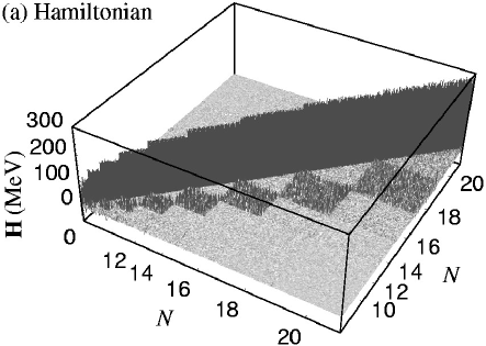
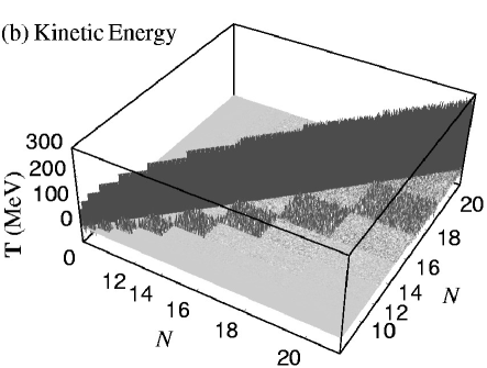
Figure 2: (a) The effective Hamiltonian of the triton with the CD-Bonn potential and $\hbar\Omega=28$ MeV. The basis is sorted according to the quantum number $N$, but the ordering within each group of states with the same $N$ is arbitrary. This ordering will be assumed in all the following figures. (b) The effective kinetic energy, which is calculated in the same way as the Hamiltonian, but with the NN interaction turned off.

The expected scaling behavior can be motivated by considering the features and results of equations (12) and (13). To this aim, the behavior of $D_{jj}$ has to be understood in more detail. Figure 2 shows the matrix elements of the effective two-body Hamiltonian and the effective two-body kinetic energy for our triton model both in the 3N basis. The effective kinetic energy is calculated in the same way as is the effective Hamiltonian, except that the NN interaction is turned off. In this case, the CD-Bonn potential is used with $N_{m}=20$ and $\hbar\Omega=28$ MeV. Comparing the kinetic energy with the full Hamiltonian, one sees that the kinetic energy dominates over the contributions from the NN interaction, especially for large HO quantum numbers. In the figure, the basis states are ordered according to their total HO quantum number $N$. The ordering within each of these groups is arbitrary.

Figure 3: The diagonal elements of the Hamiltonians and kinetic energies for ³H. The horizontal axis in the upper panel enumerates the basis states for each individual diagonal element (crosses) of the model with the CD-Bonn potential. The horizontal axis in the lower panel indicates the HO quantum number $N$ for other data. Bare T (squares) is the expectation value of the kinetic energy operator with respect to HO basis states. The remaining results are the averages of diagonal elements with the same HO quantum number $N$. From right to left, the first step of the individual diagonal elements in the upper panel corresponds to $N=20$, the next $N=18$, and so on.

The potential energy affects mostly the low-$N$ states and the cross terms among them and high-lying states. The diagonal elements of the Hamiltonian are dominant over off-diagonal elements, which confirms our expectation. It is also striking that a large number of the diagonal elements are roughly equal. The dark blocks next to the diagonals of the Hamiltonian and the kinetic energy are due to the fact that the kinetic energy operator changes the quantum number $N$ by $\pm 2$ (also 0, which corresponds to the low-amplitude diagonal blocks). Since everything is renormalized to effectively include the higher-space ($N>N_{m}$) influence, $N\pm 4,\pm 6,\ldots$ terms show up in the Hamiltonian and the kinetic energy, and they become progressively weaker towards low $N$. The above properties persist for other interactions, and other values of $\Omega$ or $N_{m}$. They are a common feature of NCSM effective Hamiltonians, at least for the 3N system.

Figure 4: The linear relation between $E_{0}$ and $\Delta E^{2}$. The upper panel is for ³H with the CD-Bonn potential, the lower one for AV18. Symbols from right to left correspond to $\widetilde{N}_{m}=10,12,\ldots,20$ for each model. The lines fit the results from $\widetilde{N}_{m}=10$ to $18$.

The behavior of the diagonal matrix elements is quantified in Fig. 3. The upper panel shows individual diagonal elements, and, again, the basis states are ordered according their HO quantum number. The lower panel plots the averages of the diagonal elements that have equal $N$. The step structure among the individual diagonal elements reflects the fact that $D_{jj}$ is roughly the same in each group of states with the same HO quantum number. The reason for the flattening for larger $N$ is two-fold. First, the number of states increases dramatically for larger $N$ and, second, the renormalization of the effective matrix elements reduces large $N$ diagonal elements. This is seen by comparing the average effective kinetic energy (circles) with the bare kinetic energy (squares), which is the expectation value of the kinetic energy operator with respect to HO basis states. For $N\leq 14$, both follow the linear ${(N+3)\over 2}\hbar\Omega$ behavior as expected. For higher $N$, the effective kinetic energy turns flatter. The figure also compares the averaged diagonal elements of the full Hamiltonians (triangles) to the ones of the kinetic energy. This again demonstrates the dominance of the kinetic energy for $N>0$. One can expect that the same behavior holds for more complex nuclei.

This structure of the effective Hamiltonian guarantees that the denominators of the second-order term in equations (12) and (13) are, to a high accuracy, equal over a wide range of $N$. Thus, we have, approximately,

$$\mathcal{E}_{0}\simeq E_{0}-\frac{1}{\alpha}\sum_{j=0}^{\hat{n}-1}\left(\psi_{0}^{\mathrm{T}}B_{j}\right)^{2}=E_{0}-\frac{1}{\alpha}\psi_{0}^{\mathrm{T}}\mathbf{BB}^{\mathrm{T}}\psi_{0},$$ (14)

where $\alpha$ is a positive constant. Since the absolute value of $E_{0}$ is much smaller than $D_{jj}$, the constant $\alpha$ should be roughly the average value of the diagonal elements with $N>\widetilde{N}_{m}$. This also means that $\alpha^{-1}$ is only weakly dependent on $E_{0}$. Neglecting higher-order perturbative terms and taking a constant true binding energy $\mathcal{E}_{0}$, it follows that $E_{0}\propto\Delta E^{2}$. This motivates a linear scaling behavior between $E_{0}$ and $\Delta E^{2}$.

Table 1: The ground state energies, $E_{0}$, of $\widetilde{\mathbf{H}}$ for ³H, their deviation from the correct result $\delta E$, and the computational time necessary for the solution. The results of the small space ($\widetilde{\mathbf{H}}$) solution are compared to the extrapolation method and the perturbative calculation using Eq. (13). All results are for CD-Bonn potential and $\hbar\Omega=28$ MeV.

		$\widetilde{\mathbf{H}}$				Extrapolation				Perturbation
$\widetilde{N}_{m}$		$E_{0}$	$\delta E$	$t$		$E_{0}$	$\delta E$	$t$		$E_{0}$	$\delta E$	$t$
12		-6.502	1493	8.2		-7.940	55	13		-7.793	202	12
14		-7.140	855	25		-8.015	-20	39		-7.906	89	28
16		-7.536	459	82		-7.980	15	120		-7.950	45	84
18		-7.869	126	210		-7.970	25	340		-7.968	27	210
20		-7.995	0	510		–	–	–		–	–	–

IV Application of the Extrapolation

Now that the linear scaling between $E_{0}$ and $\Delta E^{2}$ has been motivated, one can estimate the true binding energy $\mathcal{E}_{0}$ by a linear regression of $E_{0}$ and $\Delta E^{2}$ which are calculated with $\widetilde{N}_{m}<N_{m}$, and extrapolating it to the point where $\Delta E^{2}=0$ to estimate $\mathcal{E}_{0}$ at $N_{m}$.

The numerical results for the relation between $E_{0}$ and $\Delta E^{2}$ are shown in Fig. 4 for ³H with different NN interactions and different values of $\hbar\Omega$. $N_{m}$ is 20 in all cases, and $\widetilde{N}_{m}$ varies between 10 and 20. Additionally, linear fits to the results for $\widetilde{N}_{m}=10$ to 18 are plotted. Clearly, the linear scaling behavior is confirmed by these calculations.

Table 2: Errors in perturbative estimates of the ³H binding energy using equations (10) and (12), and the difference between extrapolated binding energies and corresponding perturbative results from equation (12). All results are for CD-Bonn potential and $\hbar\Omega=28$ MeV.

$N_{m}$	$\delta E$(Eq. [10])	$\delta E$(Eq. [12])	$\mathcal{E}_{\rm 0,e}-\mathcal{E}_{0}^{(2)}$
8	87	119	-93
10	84	167	-12
12	40	60	-17
14	52	103	3
16	27	53	-12
18	29	64	3
20	13	39	-7

Figure 5: The time consumed in the calculation in units of $t_{8}$, the time needed to solve the ground state of $\widetilde{\mathbf{H}}$ with $\widetilde{N}_{m}=8$. The diamonds mark the time it takes to extrapolate the ground state of $\mathbf{H}$ using all the ground states of $\widetilde{\mathbf{H}}({\widetilde{N}})$ with $\widetilde{N}=10\ldots\widetilde{N}_{m}$, so it is the accumulation of the time needed to solve $\widetilde{\mathbf{H}}({\widetilde{N}})$. All other symbols are as in Fig. 1.

To be more quantitative, we compare results of direct calculations, the extrapolation based on the scaling behavior, and perturbative estimates based on Eq. (13) in Table 1. The table indicates the computational efforts necessary by giving run times for different calculations. One sees that a stable extrapolation is possible starting from $\widetilde{N}_{m}=14$. The extrapolation error for larger calculations is comparable to the error of the perturbative estimates, indicating that both can be traced back to higher order terms in the perturbative expansion. In calculations for $N_{m}=30$, we have confirmed that the range of the linear behavior is extended for larger $N_{m}$. This is expected because $1/D_{jj}$ is driven by the kinetic energy and, therefore, is proportional to $1/N$ (see Fig. 3). Consequently, if $N$ is increased by one step (i.e. 2 units), then the change in $1/D_{jj}$ is of order $1/N^{2}$, which decreases with $N$. We also note that the constant $\alpha=268$ MeV for CD-Bonn with $\hbar\Omega=28$ MeV is comparable to the diagonal elements $D_{jj}$ shown in Fig. 3.

The effect of $N_{m}$ is demonstrated in Table 2, where we list errors in perturbative estimates of the ³H binding energy using equations (10) and (12). The two equations are both of the second order, and the errors tend to decrease, though not monotonically, as the model space increases. At the same time, Table 2 shows that the extrapolated binding energies converge to the results of equation (12). This is expected, because our extrapolation method, i.e., equation (14), is based on an approximation of second-order perturbation theory. The behavior of the perturbative calculations and extrapolations suggests that one can reduce the extrapolation error by increasing $N_{m}$.

The run times are also compared in Fig. 5. It is clear that perturbation theory based on Eq. (10) does not improve the timings because of the extra time needed to diagonalize $\widehat{\mathbf{H}}$. The extrapolation method for $\widetilde{N}_{m}=14$ yields sufficiently accurate results, but reduces the CPU-time by a factor of 13 compared to the full calculation. A similarly accurate perturbative calculation based on Eq. (13) is still 8 times slower, which demonstrates the usefulness of the extrapolation to extend the calculations beyond their current limits.

Figure 6: The same as Fig. 4, but for the ⁶Li nucleus. Symbols from right to left correspond to $\widetilde{N}_{m}=6,8,10$, and $12$ for each model. The lines fit the results from $\widetilde{N}_{m}=6,8$, and $10$.

We now apply the extrapolation method to the ⁶Li nucleus. The numerical results have been obtained using the Many-Fermion Dynamics (MFD) code Vary and Zheng (1994). Since we work here in a basis of slater determinants, we guarantee a $0s$ oscillator state of CM motion of our physical states by adding a CM term to equation (6), $\Lambda({\bf H}_{\rm CM}-\frac{3}{2}\hbar\Omega)$ P. Navrátil, J. P. Vary and B. R. Barrett (2000a), with $\Lambda=10$. This separates excited states of CM motion from low lying physical states. Figure 6 shows the results with $N_{m}=12$ (i.e., $10\,\hbar\Omega$ above the lowest unperturbed oscillator configuration of ⁶Li endnote24). The basis dimension of the $N_{m}=12$ calculations is 9.7 million, which is the largest model space published to date for ⁶Li. This low value of $N_{m}$ limits what $\widetilde{N}_{m}$ values one can use in the extrapolation for two reasons. Firstly, the potential energy is not negligible at small quantum numbers, so $\widetilde{N}_{m}$ should be at least greater than 4 (the ground state of ⁶Li has $N=2$). Secondly, the accuracy of the extrapolation depends on the dominance of the diagonal elements of $\mathbf{H}$, which is also weakened at small $N$. Thus, $E_{0}$ and $\Delta E^{2}$ from $\widetilde{N}_{m}=4$ calculations are not in line with those from $\widetilde{N}_{m}=6,8,10$, and 12. The extrapolation errors are 290 keV (CD-Bonn) and 220 keV (AV18). The CD-Bonn potential provides 1.1 MeV more binding than the AV18 potential. Thus, it is interesting to note that the difference between the two potentials is larger than the extrapolation error.

Figure 7: The effect of $N_{m}$ on the extrapolation error. Symbols from right to left correspond to $\widetilde{N}_{m}=N_{m}-6,\ldots,N_{m}$. The lines follow $E_{0}=\alpha_{\rm L}^{-1}\Delta E^{2}+\mathcal{E}_{0}$ and $E_{0}=\alpha_{\rm U}^{-1}\Delta E^{2}+\mathcal{E}_{0}$ for each $N_{m}$. The lines with $N_{m}=20$ are estimated from the effective kinetic energies.

The range of $\widetilde{N}_{m}$ that is suitable for extrapolation is expected to increase with $N_{m}$. This is confirmed in Fig. 7, where an additional $N_{m}=10$ calculation is made for comparison. It is seen that the results are much more linear for the case $N_{m}=12$. Figure 7 also demonstrates why a higher value of $N_{m}$ is likely to produce a smaller extrapolation error. We can estimate the lower and upper bounds of the constant $\alpha$, $(\alpha_{\rm L},\alpha_{\rm U})$, in equation (14) using effective kinetic energies and unperturbed ground state energies $E_{0}$ for $\widetilde{N}_{m}=N_{m}-2$ and $N_{m}-6$. The results of $\widetilde{N}_{m}$ calculations are consistent with second-order perturbation theory, because they are roughly bounded by $\alpha_{\rm L}$ and $\alpha_{\rm U}$ for each $N_{m}$. The opening angle between the lines of slope $\alpha_{\rm L}^{-1}$ and $\alpha_{\rm U}^{-1}$ decreases as $N_{m}$ increases. Hence, we expect to reduce the extrapolation error by increasing $N_{m}$.

V Conclusions and Outlook

Because of the need for a large basis space to achieve accurate results, even light nuclei require a significant amount of computing resources to be investigated in the NCSM. We have justified and verified an extrapolation method for NCSM calculations. It is reliable, and can provide good estimates of large-space results from several small-space calculations. Sometimes, it may be the only means for getting a useful estimate of the NCSM result for otherwise unachievable large model spaces.

The extrapolation formula proposed in Ref. Mizusaki and Imada (2003) agrees in leading order with our Eq. (14). We would like to emphasize that the linear scaling between $E_{0}$ and $\Delta E^{2}$ is based on perturbation theory. It is not an expansion in terms of $\Delta E^{2}E^{-2}_{0}$, because $\Delta E^{2}$ can be much greater than $E^{2}_{0}$ in the NCSM (see Fig. 4). The reasoning behind our extrapolation method is probably applicable only to NCSM calculations, because we have explicitly made use of the structure of the Hamiltonian in our derivation. The linear scaling between $E_{0}$ and $\Delta E^{2}$ relies on the flattening of the diagonal elements of the effective Hamiltonian (dominated by the kinetic energy) as $N$ approaches $N_{m}$. With this behavior, the energy denominator in equation (12) can be approximated by a constant $\alpha$.

Generally speaking, extrapolation methods depend not only on the structure of the Hamiltonian but also on the truncation scheme that is used to produce an approximate state. Different truncation schemes may lead to different scaling behavior Mizusaki and Imada (2003). The traditional phenomenological shell model does not generate the structure of the Hamiltonian that is advantageous for our method. Specifically, in calculations with a core diagonal dominance is reduced since energies relative to a core are obtained. For realistic mean field potentials, the single particle spectrum does not rise as fast as an oscillator spectrum which itself does not rise as fast as the kinetic spectrum in an oscillator basis. Hence, the diagonal dominance we have in the NCSM is much stronger than the traditional shell model, and our method probably cannot be applied to the traditional shell model without modifications. On the other hand, the methods for the traditional shell model do not necessarily apply to the NCSM either. In fact, it is evident from Fig. 6 that a quadratic fit Mizusaki and Imada (2003) to the $\widetilde{N}_{m}=6$, 8, and 10 results will yield a significantly larger error.

From Table 2 we have learned that for small model spaces there are two competing sources of inaccuracy: one in the perturbation theory result and the other in the extrapolated result. We have shown that the extrapolated result is converging to the perturbation theory result, equation (12). In Table 2 one sees that the deviation of equation (12) and the extrapolation is already small even for relatively small values of $N_{m}$, e.g., $N_{m}=10$. Since perturbation theory requires larger $N_{m}$, around 16, to give estimates of similar accuracy, we can conclude that overall our results are probably dominated by errors due to perturbation theory.

This method, like NCSM calculations themselves, is limited by the size of the model-space, because $\Delta E^{2}$ has to be evaluated in the full $P$ space. Nevertheless, it has been shown to be a valuable tool. Its power is based on the much smaller dimension of the $\mathbf{B}$ matrix compared to the full matrix for the Hamiltonian operator. Calculations for even larger model spaces will become possible once we make explicit use of the small dimension of the $\mathbf{B}$ matrix in our codes.

In Figs. 4 and 6, we observe that the extrapolation error, i.e., $\delta E=E_{0}-\mathcal{E}_{0}$, at $\Delta E^{2}=0$ is quite small compared with differences in exact results of $\mathcal{E}_{0}$ for various values of $\hbar\Omega$ or choices of potentials. Therefore, the extrapolation can also serve as a way to estimate the uncertainties of NCSM results arising from $\hbar\Omega$ dependence and choices of interactions. This will be an important application of our method in future investigations of nuclei within the NCSM.

References

- Pieper and Wiringa (2001) S. C. Pieper and R. B. Wiringa, Ann. Rev. Nucl. Part. Sci. 51, 53 (2001).
- Y. Suzuki and K. Varga (1998) Y. Suzuki and K. Varga, Stochastical variational approach to Quantum-Mechanical Few-Body Problems, vol. m54 of Lecture Notes in Physics (Springer-Verlag, Berlin, 1998).
- S. E. Koonin, D. J. Dean and K. Langanke (1997) S. E. Koonin, D. J. Dean and K. Langanke, Phys. Rep. 278, 1 (1997).
- Navrátil and Ormand (2002) P. Navrátil and W. E. Ormand, Phys. Rev. Lett. 88, 152502 (2002).
- Kamada et al. (2001) H. Kamada, A. Nogga, W. Glöckle, E. Hiyama, M. Kamimura, K. Varga, Y. Suzuki, M. Viviani, A. Kievsky, S. Rosati, et al., Phys. Rev. C 64, 044001 (2001).
- B. R. Barrett, B. Mihaila, S. C. Pieper, R. B. Wiringa (2003) B. R. Barrett, B. Mihaila, S. C. Pieper, R. B. Wiringa, Nucl. Phys. News 13, 20 (2003).
- P. Navrátil, J. P. Vary and B. R. Barrett (2000a) P. Navrátil, J. P. Vary and B. R. Barrett, Phys. Rev. C 62, 054311 (2000a).
- Mizusaki and Imada (2002) T. Mizusaki and M. Imada, Phys. Rev. C 65, 064319 (2002).
- Mizusaki and Imada (2003) T. Mizusaki and M. Imada, Phys. Rev. C 67, 041301(R) (2003).
- Navrátil et al. (2000) P. Navrátil, G. P. Kamuntavičius, and B. R. Barrett, Phys. Rev. C 61, 044001 (2000).
- Suzuki and Lee (1980) K. Suzuki and S. Y. Lee, Progr. of Theor. Phys. 64, 2091 (1980).
- K. Suzuki (1982) K. Suzuki, Progr. of Theor. Phys. 68, 246 (1982).
- P. Navrátil, J. P. Vary and B. R. Barrett (2000b) P. Navrátil, J. P. Vary and B. R. Barrett, Phys. Rev. Lett. 84, 5728 (2000b).
- S. Okubo (1954) S. Okubo, Progr. Theor. Phys. 12, 603 (1954).
- Navrátil and Ormand (2003) P. Navrátil and W. E. Ormand, Phys. Rev. C 68, 034305 (2003).
- Marsden et al. (2002a) D. Marsden, P. Navrátil, S. Coon, and B. Barrett, Phys. Rev. C 66, 044007 (2002a).
- Lipkin (1958) H. J. Lipkin, Phys. Rev. 109, 2071 (1958).
- Marsden et al. (2002b) D. C. J. Marsden, P. Navrátil, S. A. Coon, and B. R. Barrett, Phys. Rev. C 66, 044007 (2002b).
- Nogga et al. (2002) A. Nogga, H. Kamada, W. Glöckle, and B. R. Barrett, Phys. Rev. C 65, 054003 (2002).
- Nogga et al. (2003) A. Nogga, A. Kievsky, H. Kamada, W. Glöckle, L. E. Marcucci, S. Rosati, and M. Viviani, Phys. Rev. C 67, 034004 (2003).
- R. Machleidt (2001) R. Machleidt, Phys. Rev. C 63, 024001 (2001).
- R. B. Wiringa et al. (1995) R. B. Wiringa, V. G. J. Stoks, and R. Schiavilla, Phys. Rev. C 51, 38 (1995).
- Vary and Zheng (1994) J. P. Vary, Many-fermion-dynamics shell-model code (1992), (unpublished); J. P. Vary and D. C. Zheng, ibid (1994).