Nonequilibrium Quantum-Field Dynamics and Off-Shell Transport for $\phi^{4}$-theory in 2+1 dimensions

Abstract

We solve the Kadanoff-Baym equations for nonequilibrium initial configurations of the $\phi^{4}$-theory in 2+1 dimensions and compare to explicit solutions of generalized transport equations for the same theory. The latter transport equations are derived from the Kadanoff-Baym equation in a first order gradient expansion in phase space and explicitly retain the off-shell dynamics as inherent in the time-dependent spectral functions. The solutions of these equations compare very well with the exact solutions of the full Kadanoff-Baym equations with respect to the occupation numbers of the individual modes, the spectral evolution as well as the chemical equilibration process. Furthermore, the proper equilibrium off-shell distribution is reached for large times contrary to the quasiparticle Boltzmann limit. We additionally present a direct comparison of the solution of the generalized transport equations in the Kadanoff-Baym and Botermans-Malfliet form; both solutions are found to agree very well with each other.

PACS: 06.60.+w; 05.70.Ln; 11.10.Wx; 24.10.-i; 25.75.-q

Keywords: Many-body theory; finite temperature field theory; out-of-equilibrium quantum field theory; nonequilibrium statistical physics; relativistic heavy-ion collisions

1 Introduction

Nonequilibrium many-body theory or quantum-field theory has become a major topic of research for transport processes in nuclear physics, in cosmological particle physics as well as condensed matter physics. In particular the dynamics of heavy-ion collisions at various bombarding energies – as representative of complex systems with strongly interacting particles or fields – has always been a major motivation for research on nonequilibrium quantum many-body physics. The initial state of such collisions represents an extreme nonequilibrium situation, whereas the final state might exhibit a certain degree of thermalization in central reactions. Indeed, at the presently highest energy heavy-ion collider experiments at the Relativistic Heavy-Ion Collider (RHIC), where one expects to create experimentally an intermediate state of deconfined matter (denoted as quark-gluon plasma (QGP)), there are experimental signatures for an early thermalization accompanied with the generation of a very large pressure. Such a rapid thermalization cannot be explained by binary on-shell parton scattering using cross sections from perturbative QCD (pQCD) [1]. Presently open questions in high-energy nuclear physics are, if i) the quantum off-shell equilibration proceeds much faster than ordinary two-body on-shell Boltzmann kinetics and if ii) multi-parton interactions play a decisive role.

We here primarily focus on the first issue and present solutions for the full quantum time evolution of nonequilibrium $\phi^{4}$-theory in 2+1 dimensions in comparison to generalized off-shell transport equations – derived in the last years [2, 3] – as well as the on-shell quasiparticle Boltzmann limit. The scalar $\phi^{4}$-theory, of cause, is much simpler than a non-abelian gauge-field theory like QCD, however, provides a suitable testing ground for approximation schemes to the field theoretical many-body problem.

We recall that a proper basis for nonequilibrium quantum many-body physics is provided by the closed-time-path (CTP) functional integral (‘Schwinger-Keldysh’ [4, 5, 6, 7, 8]) formalism. The essential merit of this real-time Green function technique is its applicability to all kind of quantum nonequilibrium phenomena. In this context the most prominent role is played by the causal Dyson-Schwinger equations of motion for the one-particle Green functions, i.e. the Kadanoff-Baym (KB) equations [9, 10, 11, 12, 13, 14]. The latter, furthermore, have served as a basis for the derivation of generalized transport equations, which play the central role in almost all practical simulations of nonrelativistic and relativistic nonequilibrium many-body systems. In the past, a major impetus has been to derive semiclassical Boltzmann-like transport equations within the standard quasiparticle approximation [15, 16, 17, 18]. More recently, off-shell extensions by means of a gradient expansion in the space-time inhomogeneities have been formulated for several systems: for a relativistic electron-photon plasma [19], for transport of electrons in a metal with external electrical field [20] and in semiconductors [13, 21], for transport of nucleons in heavy-ion reactions at intermediate energies [22], for transport of particles in $\phi^{4}$-theory [12, 23] as well as for transport of partons in high-energy heavy-ion reactions [24, 25, 26, 27].

Within all these derivations the particle self-energies – entering the KB equations – have to fulfill consistency relations in order to preserve symmetries of the fundamental Lagrangian [9, 28, 29]. In this respect an elegant way for achieving selfconsistency is provided by the two-particle-irreducible (2PI) effective action [12, 30, 31]. Including the background field and the correlation function on the same footing, collisions can be naturally included by taking into account contributions beyond the leading mean-field order of the generating functional. Due to the construction in terms of full Green functions this method ensures the validity of all essential conservation laws.

Moreover, in the nuclear physics context the quantum dynamics of the spectral function is a lively discussed issue in the microscopic modeling of hadronic resonances with a broad mass distribution. This is of particular relevance for simulations of heavy-ion reactions where e.g. the $\Delta$-resonance or the $\rho$-meson already show a large decay width in vacuum. Especially the $\rho$ vector meson is a promising hadronic particle for showing possible in-medium modifications in hot and compressed nuclear matter (see e.g. [32, 33, 34]), since the leptonic decay products only interact electromagnetically. Hence, a consistent formulation for the transport of extremely short-lived particles beyond the standard quasiparticle approximation is needed. On the one side, there exist purely formal developments starting from a first order gradient expansion of the underlying KB equations [9, 35, 36, 37, 38], while on the other side already first practical realizations for various questions have emerged [2, 3, 39, 40, 41]. However, a fully ab initio investigation for a strongly interacting field theoretical system in 3+1 dimensions –without any further approximations – does not exist so far as well as a rigorous demonstration of the reliability of the different schemes for off-shell transport dynamics.

Although the Kadanoff-Baym equation has been of wide interest, (numerical) investigations of its full solution are rather scarce for strongly interacting systems. First studies in the nuclear physics context have been performed by Danielewicz [42], who investigated the initial distribution of two occupied non-relativistic Fermi spheres in momentum space for spatially homogeneous systems. In comparison to a standard on-shell semiclassical Boltzmann equation the full quantum Kadanoff-Baym solution showed a larger collective relaxation time which was attributed to quantum interference and off-shell effects. Similar quantum modifications in the equilibration and momentum relaxation have been found in [15] and for a relativistic situation in Ref. [43]. Furthermore, the spectral properties of nuclear systems in the nonrelativistic regime have been first examined on the basis of the KB equations in Refs. [44, 45]. We mention that solutions of quantum transport equations for semiconductors [13, 46] – to explore relaxation phenomena on short time and distance scales – have become also a very active field of research (cf. Ref. [47] for a recent overview).

The basic aim of our present study is to examine exact solutions of the KB equations for strongly interacting (scalar) fields in comparison to the solution of generalized kinetic equations as obtained from a gradient expansion of the full Kadanoff-Baym equation. Although such generalized transport equations have already been used in the past, a check against the full solution is still lacking. To this aim we will investigate the scalar $\phi^{4}$-theory for the case of 2+1 space-time dimensions since – first of all – it superceeds the rather artificial structure of the $\phi^{4}$-theory in 1+1 dimensions, that has been investigated before. In the latter case on-shell scattering processes are (col-)linear and thus do not lead to an equilibration in accordance with an appropriate change of the momentum distribution. Thermalization in 1+1 dimensions is only mediated by off-shell scattering processes. This is a rather unusual situation, since it is known from the investigation of heavy-ion collisions by means of quantum kinetic theories, that binary on-shell scattering plays an important role. In the 2+1 dimensional case both, on-shell and off-shell collisions influence the equilibration behaviour. Thus the theory in 2+1 dimensions is a well-suited laboratory in order to investigate the differences between the full Kadanoff-Baym theory and approximate schemes as given by the on-shell Boltzmann limit or by generalized off-shell transport equations. Furthermore, the divergence structure of the $\phi^{4}$-theory in 2+1 dimensions allows for a controlled renormalization procedure because only two self-energies – containing pure vacuum parts of Green functions – diverge in the ultraviolet regime. Thus the renormalization can be performed equivalently to the standard zero temperature vacuum case. This is different in 3+1 dimensions, where complete classes of self-energies are divergent, which incorporate non-vacuum parts of the Green functions as well. In the latter case more involved renormalization schemes should be used analogous to those constructed for self-consistent approximations at finite temperature [48, 49, 50].

Our work is organized as follows: In Section 2 we will present the relevant equations for the nonequilibrium dynamics in case of the $\phi^{4}$-theory and provide the Kadanoff-Baym equations within the three-loop approximation of the 2PI effective action. Furthermore, we briefly review the derivation of generalized transport equations and discuss different limits. Section 3 is devoted to numerical studies on equilibration phenomena within the full Kadanoff-Baym theory (cf. Ref. [51]) in comparison to the generalized transport equations in either Kadanoff-Baym (KB) form [9] or Botermans-Malfliet (BM) approximation [22]. We will also address the differences in the solutions of the two different versions (KB and BM) of the off-shell transport theory and explore the validity of the gradient expansion employed. We close this work in Section IV with a summary of our results and an outlook on future extensions.

2 Derivation of Generalized Transport Equations

In continuation of our previous study in Ref. [51] we investigate the out-of-equilibrium quantum dynamics of interacting scalar fields by the example of the $\phi^{4}$-theory that allows to test theoretical approximations in a variety of aspects [52, 53, 54, 55]. Its Lagrangian density is given by $(x=(t,\vec{x}))$

$${\cal L}(x)\;=\;\frac{1}{2}\,\partial_{\mu}\phi(x)\,\partial^{\mu}\phi(x)\>-\>\frac{1}{2}\,m^{2}\,\phi^{2}(x)\>-\>\frac{\lambda}{4!}\,\phi^{4}(x)\;,$$ (1)

where $m$ denotes the ‘bare’ mass and $\lambda$ is the coupling constant determining the interaction strength of the scalar fields.

For the derivation and investigation of generalized transport equations we first have to specify the necessary notations and the explicit form of the Kadanoff-Baym equations. Though the details of the derivation are given in Ref. [51] we briefly recall the main steps in order to keep the paper self-containt.

2.1 The Kadanoff-Baym Equations

A natural starting point for nonequilibrium quantum theory is provided by the closed-time-path (CTP) method. Here all quantities are given on a special real-time contour with the time argument running from $-\infty$ to $+\infty$ on the chronological branch $(+)$ and returning from $+\infty$ to $-\infty$ on the anti-chronological branch $(-)$. In particular the path-ordered Green functions are defined as $(x_{1}=(t_{1},\vec{x}_{1}),\;x_{2}=(t_{2},\vec{x}_{2}))$

$$G(x_{1},x_{2}) = \langle\>T^{p}\,\{\,\phi(x_{1})\>\phi(x_{2})\,\}\,\rangle$$

$$= \Theta_{p}(t_{1}-t_{2})\;\langle\,\phi(x_{1})\>\phi(x_{2})\,\rangle\;+\;\Theta_{p}(t_{2}-t_{1})\;\langle\,\phi(x_{2})\>\phi(x_{1})\,\rangle\,,$$

where the operator $T^{p}$ orders the field operators according to the position of their arguments on the real-time path as accomplished by the path step-functions $\Theta_{p}$

$$\Theta_{p}(t_{1}-t_{2})\;=\;\left\{\begin{array}[]{cl}1\,,&{\rm if\;\>}t_{1}\;\>{\rm is\;later\;on\;the\;contour\;as\;\>}t_{2}\,,\\[11.38092pt] 0\,,&{\rm if\;\>}t_{2}\;\>{\rm is\;earlier\;on\;the\;contour\;as\;\>}t_{1}\,.\end{array}\right.$$ (5)

The expectation value in (2.1) is taken with respect to some given density matrix $\rho_{0}$, which is constant in time, while the operators in the Heisenberg picture contain the whole information of the time dependence of the nonequilibrium system.

Self-consistent equations of motion for these Green functions can be obtained with help of the two-particle-irreducible (2PI) effective action $\Gamma[G]$, which is given by the double Legendre transform of the generating functional of connected Green functions $W$ with respect to the local and bilinear external sources [51]. The functional $\Phi$, which is the sum of all closed 2PI diagrams built up by full propagators $G$ (and bare vertices) [28, 56, 57], determines the resummed self-energy by functional variation as

$$\Sigma(x_{1},x_{2})\;=\;2i\,\frac{\delta\Phi}{\delta G(x_{2},x_{1})}\>.$$ (6)

In general, the self-energy $\Sigma$ contains a singular contribution $\Sigma^{\delta}$ on the contour and a non-local part, which can be expressed by a sum over $\Theta_{p}$-functions

$$\Sigma(x_{1},x_{2}) = \Sigma^{\delta}(x_{1})\;\delta_{p}^{(d+1)}(x_{1}\!-\!x_{2})$$

$$+\;\Theta_{p}(t_{1}\!-\!t_{2})\>\Sigma^{>}(x_{1},x_{2})\;+\;\Theta_{p}(t_{2}\!-\!t_{1})\>\Sigma^{<}(x_{1},x_{2})\,.\phantom{a}$$

Here the $\delta_{p}$-function on the closed-time-path is defined as

$$\delta_{p}^{(d+1)}(x_{1}-x_{2})\;=\;\delta_{p}(t_{1}-t_{2})\;\;\delta^{(d)}(\vec{x}_{1}-\vec{x}_{2})\,,$$ (8)

$$\delta_{p}(t_{1}-t_{2})\;=\;\left\{\begin{array}[]{cl}\phantom{-}\delta(t_{1}-t_{2})\,,&{\rm if\;both\;\>}t_{1}\;\>{\rm and\;\>}t_{2}\;\>{\rm are\;on\;the\;upper\;(+)\;branch}\,,\\[5.69046pt] -\delta(t_{1}-t_{2})\,,&{\rm if\;both\;\>}t_{1}\;\>{\rm and\;\>}t_{2}\;\>{\rm are\;on\;the\;lower\;(-)\;branch}\,,\\[5.69046pt] 0\,,&{\rm in\;other\;cases}\,,\end{array}\right.$$ (10)

in accordance with the contour integration while $d$ denotes the spatial dimension of the problem. The functional $\Phi$ allows – by restricting to a particular set of diagrams – for the construction of effective theories, which are conserving and thermodynamically consistent [28, 58]. In our present calculations we will take into account contributions up to the three-loop order for the $\Phi$-functional (cf. Fig. 1 in Ref. [51]). Whereas the self-energies are defined by (6) the evolution of the Green function is determined by the stationarity condition $\delta\Gamma/\delta G=0$ [37, 51].

For actual calculations it is advantageous to change to a single-time representation for the Green functions and (the non-local part of) the self-energies defined on the closed-time-path. In line with the position of the coordinates on the contour there exist four different two-point functions

$$i\,G^{c}(x_{1},x_{2}) = i\,G^{++}(x_{1},x_{2})\;\;=\;\;i\,G(x_{1}^{+},x_{2}^{+})\;\;=\;\;\langle\,T^{c}\,\{\,\phi(x_{1})\>\phi(x_{2})\,\}\,\rangle\,,\phantom{aaa}$$ (11)

$$i\,G^{<}(x_{1},x_{2}) = i\,G^{+-}(x_{1},x_{2})\;\;=\;\;i\,G(x_{1}^{+},x_{2}^{-})\;\;=\;\;\;\;\;\;\>\langle\,\{\,\phi(x_{2})\>\phi(x_{1})\,\}\,\rangle\,,$$

$$i\,G^{>}(x_{1},x_{2}) = i\,G^{-+}(x_{1},x_{2})\;\;=\;\;i\,G(x_{1}^{-},x_{2}^{+})\;\;=\;\;\>\;\;\;\>\langle\,\{\,\phi(x_{1})\>\phi(x_{2})\,\}\,\rangle\,,$$

$$i\,G^{a}(x_{1},x_{2}) = i\,G^{--}(x_{1},x_{2})\;\;=\;\;i\,G(x_{1}^{-},x_{2}^{-})\;\;=\;\;\langle\,T^{a}\,\{\,\phi(x_{1})\>\phi(x_{2})\,\}\,\rangle\,.$$

Here $T^{c}\,(T^{a})$ represent the (anti-)time-ordering operators in case of both arguments lying on the (anti-)chronological branch of the real-time contour. These four functions are not independent of each other. In particular the non-continuous functions $G^{c}$ and $G^{a}$ are built up by the Wightman functions $G^{>}$ and $G^{<}$ and the usual $\Theta$-functions in the time coordinates as

$$G^{c}(x_{1},x_{2}) = \Theta(t_{1}-t_{2})\;G^{>}(x_{1},x_{2})\>+\>\Theta(t_{2}-t_{1})\;G^{<}(x_{1},x_{2})\,,$$ (12)

$$G^{a}(x_{1},x_{2}) = \Theta(t_{2}-t_{1})\;G^{>}(x_{1},x_{2})\>+\>\Theta(t_{1}-t_{2})\;G^{<}(x_{1},x_{2})\,.$$

By fixing the time arguments of the Green functions on different branches of the contour and resolving the time structure of the path-ordered quantities we obtain the Kadanoff-Baym equations for the time evolution of the Wightman functions [23, 51, 54]:

$$-\left[\partial_{\mu}^{x_{1}}\partial_{x_{1}}^{\mu}\!+m^{2}\right]\,G^{\gtrless}(x_{1},x_{2}) = \Sigma^{\delta}(x_{1})\;G^{\gtrless}(x_{1},x_{2})$$

$$\!\!\!\!\!\!\!\!\!\!\!\!\!\!\!\!\!\!\!\!+\int_{t_{0}}^{t_{1}}\!\!\!\!\!dz_{0}\int\!\!d^{d}\!z\;\;\left[\,\Sigma^{>}(x_{1},z)-\Sigma^{<}(x_{1},z)\,\right]\>G^{\gtrless}(z,x_{2})$$

$$\!\!\!\!\!\!\!\!\!\!\!\!\!\!\!\!\!\!\!\!-\int_{t_{0}}^{t_{2}}\!\!\!\!\!dz_{0}\int\!\!d^{d}\!z\;\;\,\Sigma^{\gtrless}(x_{1},z)\>\left[\,G^{>}(z,x_{2})-G^{<}(z,x_{2})\,\right]\,,$$

$$-\left[\partial_{\mu}^{x_{2}}\partial_{x_{2}}^{\mu}\!+m^{2}\right]\,G^{\gtrless}(x_{1},x_{2}) = \Sigma^{\delta}(x_{2})\;G^{\gtrless}(x_{1},x_{2})$$

$$\!\!\!\!\!\!\!\!\!\!\!\!\!\!\!\!\!\!\!\!+\int_{t_{0}}^{t_{1}}\!\!\!\!\!dz_{0}\int\!\!d^{d}\!z\;\;\left[\,G^{>}(x_{1},z)-G^{<}(x_{1},z)\,\right]\>\Sigma^{\gtrless}(z,x_{2})$$

$$\!\!\!\!\!\!\!\!\!\!\!\!\!\!\!\!\!\!\!\!-\int_{t_{0}}^{t_{2}}\!\!\!\!\!dz_{0}\int\!\!d^{d}\!z\;\;\,G^{\gtrless}(x_{1},z)\>\left[\,\Sigma^{>}(z,x_{2})-\Sigma^{<}(z,x_{2})\,\right]\,.$$

Within the three-loop approximation for the 2PI effective action $\Phi$ we get two different self-energies: In leading order of the coupling constant only the local tadpole diagram contributes and leads to the generation of an effective mass for the field quanta. This self-energy (in coordinate space) is given by [51]

$$\Sigma^{\delta}(x)\;=\;\frac{\lambda}{2}\;i\>G^{<}(x,x)\>.$$ (14)

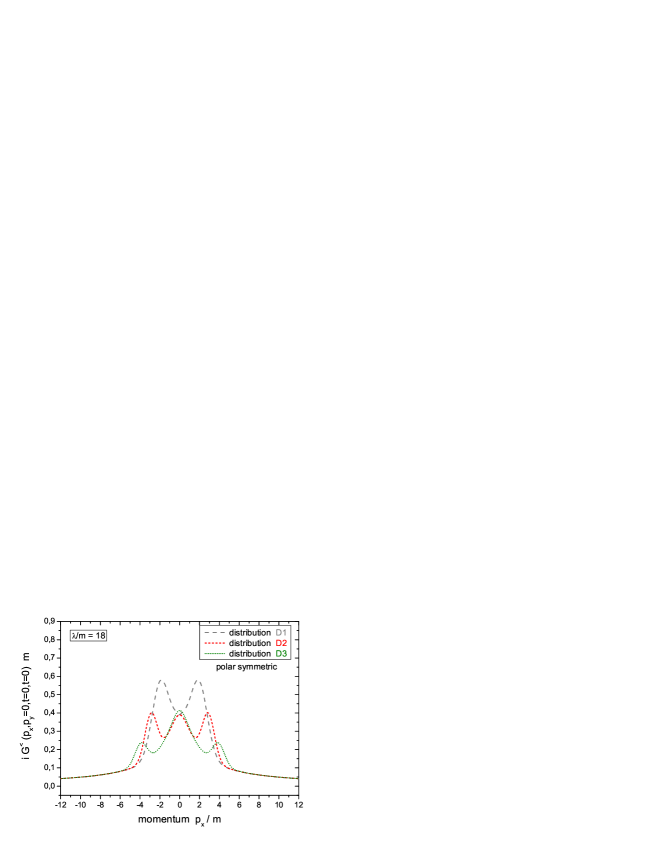
Figure 1: Initial momentum distributions for the initializations D1, D2 and D3. For the polar symmetrical settings in momentum space the distributions are shown as function of $p_{x}$ (for $p_{y}=0$).

Figure 2: Initial equal-time Green functions for the initializations D1, D2 and D3. The equal-time Green functions are displayed for polar symmetric systems as a function of $p_{x}$ (for $p_{y}=0$) with coupling constant $\lambda/m=18$.

In next order in the coupling constant (i.e. $\lambda^{2}$) the non-local sunset self-energy (cf. Fig. 2 in [51]) enters the time evolution as

$$\Sigma^{\gtrless}(x_{1},x_{2})\;=\;-\frac{\lambda^{2}}{6}\;G^{\gtrless}(x_{1},x_{2})\;G^{\gtrless}(x_{1},x_{2})\;G^{\lessgtr}(x_{2},x_{1})\;=\;-\frac{\lambda^{2}}{6}\;\left[\,G^{\gtrless}(x_{1},x_{2})\,\right]^{3}\!\!\!.\phantom{a}$$ (15)

Thus the Kadanoff-Baym equation (2.1) in our case includes the influence of a mean-field on the particle propagation – generated by the tadpole diagram – as well as scattering processes as inherent in the sunset diagram.

The Kadanoff-Baym equation (2.1) describes the full quantum nonequilibrium time evolution on the two-point level for a system prepared at an initial time $t_{0}$, i.e. when higher order correlations are discarded. The causal structure of this initial value problem is obvious since the time integrations are performed over the past up to the actual time $t_{1}$ (or $t_{2}$, respectively) and do not extend to the future.

Furthermore, also linear combinations of the Green functions in single-time representation are of interest and will be exploited for the spectral properties of the system later on. The retarded Green function $G^{R}$ and the advanced Green function $G^{A}$ are given as

$$G^{R}(x_{1},x_{2}) = \phantom{-}\,\Theta(t_{1}-t_{2})\;\left[\,G^{>}(x_{1},x_{2})-G^{<}(x_{1},x_{2})\,\right]$$

$$= \phantom{-}\,\Theta(t_{1}-t_{2})\;\langle\,\left[\,\phi(x_{1})\,,\,\phi(x_{2})\,\right]_{-}\,\rangle$$

$$= \phantom{-}\,G^{c}(x_{1},x_{2})\>-\>G^{<}(x_{1},x_{2})\;\>=\;\>G^{>}(x_{1},x_{2})\>-\>G^{a}(x_{1},x_{2})\,,$$

$$G^{A}(x_{1},x_{2}) = -\,\Theta(t_{2}-t_{1})\;\left[\,G^{>}(x_{1},x_{2})-G^{<}(x_{1},x_{2})\,\right]$$

$$= -\,\Theta(t_{2}-t_{1})\;\langle\,\left[\,\phi(x_{1})\,,\,\phi(x_{2})\,\right]_{-}\,\rangle$$

$$= \phantom{-}\,G^{c}(x_{1},x_{2})\>-\>G^{>}(x_{1},x_{2})\;\>=\;\>G^{<}(x_{1},x_{2})\>-\>G^{a}(x_{1},x_{2})\,.$$

These Green functions contain exclusively spectral, but no statistical information of the system. Their time evolution is determined by Dyson-Schwinger equations and given by (cf. Ref. [51])

$$-\left[\partial_{\mu}^{x_{1}}\partial_{x_{1}}^{\mu}\!+m^{2}+\Sigma^{\delta}(x_{1})\right]\,G^{R}(x_{1},x_{2})\;=\;$$ (18)

$$\qquad\qquad\qquad\qquad\qquad\delta^{(d+1)}(x_{1}\!-\!x_{2})\>+\>\int\!d^{d+1}\!z\;\;\Sigma^{R}(x_{1},z)\;\;G^{R}(z,x_{2})\,,$$

$$-\left[\partial_{\mu}^{x_{1}}\partial_{x_{1}}^{\mu}\!+m^{2}+\Sigma^{\delta}(x_{1})\right]\,G^{A}(x_{1},x_{2})\>=\>$$ (19)

$$\qquad\qquad\qquad\qquad\qquad\delta^{(d+1)}(x_{1}\!-\!x_{2})\>+\>\int\!d^{d+1}\!z\;\;\Sigma^{A}(x_{1},z)\;\;G^{A}(z,x_{2})\,,$$

where the retarded and advanced self-energies $\Sigma^{R}$, $\Sigma^{A}$ are defined via $\Sigma^{>}$, $\Sigma^{<}$ similar to the Green functions (2.1) and (2.1). Thus the retarded (advanced) Green functions are determined by retarded (advanced) quantities, only.

2.2 Generalized transport equations

The derivation of generalized transport equations has been presented before in Refs. [2, 9, 14, 22, 35, 36, 37, 38]. We here briefly repeat the derivation in order to introduce the necessary notations and to work out the differences in the Kadanoff-Baym [9] and Botermans-Malfliet [22] scheme that will be investigated in Section 3.

We start by rewriting the Kadanoff-Baym equation for the Wightman functions in coordinate space ($x_{1}\!=\!(t_{1},\vec{x}_{1}),x_{2}\!=\!(t_{2},\vec{x}_{2})$) (2.1) as

$$[\,\partial^{\mu}_{x_{1}}\partial_{\mu}^{x_{1}}+m^{2}+\Sigma^{\delta}(x_{1})\,]\;\>iG^{\gtrless}(x_{1},x_{2})\;=\;i\,I_{1}^{\gtrless}(x_{1},x_{2})\,.$$ (20)

The collision terms on the r.h.s. of (20) are given in $D=d+1$ space-time dimensions by convolution integrals over coordinate space self-energies and Green functions:

$$I_{1}^{\gtrless}(x_{1},x_{2})\>=\> - \!\!\int_{t_{0}}^{t_{1}}\!\!\!d^{D}\!z\;\;\left[\,\Sigma^{>}(x_{1},z)-\Sigma^{<}(x_{1},z)\,\right]\;\;G^{\gtrless}(z,x_{2})$$

$$+ \!\!\int_{t_{0}}^{t_{2}}\!\!\!d^{D}\!z\;\;\Sigma^{\gtrless}(x_{1},z)\;\;\left[\,G^{>}(z,x_{2})-G^{<}(z,x_{2})\,\right]\,.$$

In the general case of an arbitrary (scalar) quantum field theory $\Sigma^{\delta}$ is the local (non-dissipative) part of the path self-energy while $\Sigma^{\gtrless}$ resemble the non-local collisional self-energy contributions. In the representation (2.2) the integration boundaries are exclusively given for the time coordinates since the integration over the spatial coordinates extends over the whole spatial volume from $-\infty$ to $+\infty$.

Since transport theories are formulated in phase-space one changes to the Wigner representation via Fourier transformation with respect to the rapidly varying (’intrinsic’) relative coordinate $\Delta x=x_{1}-x_{2}$ and treats the system evolution in terms of the (’macroscopic’) mean space-time coordinate $x=(x_{1}+x_{2})/2$ and the four-momentum $p=(p_{0},\vec{p})$. The functions in Wigner space are obtained as

$$\bar{F}(p,x)\;=\;\int_{-\infty}^{\infty}\!\!\!d^{D}\!\Delta x\;\;\;e^{+i\>\Delta x_{\mu}\>p^{\mu}}\;\;F(x_{1}=x+\Delta x/2,\,x_{2}=x-\Delta x/2)\,.$$ (22)

For the formulation of transport theory in the Wigner representation we have to focus not only on the transformation properties of ordinary two-point functions as given in (22), but also of convolution integrals as appearing in Eq. (2.2). A convolution integral in $D$ dimensions (for arbitrary functions $F,G$),

$$H(x_{1},x_{2})\;=\;\int_{-\infty}^{\infty}\!\!\!d^{D}\!z\;\;F(x_{1},z)\;\;G(z,x_{2})$$ (23)

transforms as

$$\bar{H}(p,x) = \int_{-\infty}^{\infty}\!\!\!d^{D}\!\Delta x\;\;\;e^{+i\>\Delta x_{\mu}\>p^{\mu}}\;\;H(x_{1},x_{2})$$

$$= \int_{-\infty}^{\infty}\!\!\!d^{D}\!\Delta x\;\;\;e^{+i\>\Delta x_{\mu}\>p^{\mu}}\;\;\int_{-\infty}^{\infty}\!\!\!d^{D}\!z\;\;F(x_{1},z)\;\;G(z,x_{2})$$

$$= \left.\;e^{+i\,\frac{1}{2}\,(\partial_{p^{\phantom{\prime}}}^{\mu}\!\!\cdot\>\partial^{x^{\prime}}_{\mu}\>-\;\partial_{x^{\phantom{\prime}}}^{\mu}\!\!\cdot\>\partial^{p^{\prime}}_{\mu})}\;\>\left[\;\bar{F}(p,x)\;\;\bar{G}(p^{\prime},x^{\prime})\;\right]\right|_{x^{\prime}=x,\>p^{\prime}=p}\;.$$

In accordance with the standard assumption of transport theory we assume that all functions only smoothly evolve in the mean space-time coordinates and thus restrict to first order derivatives. All terms proportional to second or higher order derivatives in the mean space-time coordinates (also mixed ones) will be dropped. Thus the Wigner transformed convolution integrals (23) are given in first order gradient approximation by,

$$\bar{H}(p,x)\;=\;\bar{F}(p,x)\;\;\bar{G}(p,x)\;+\;i\,\frac{1}{2}\>\{\,\bar{F}(p,x)\,,\,\bar{G}(p,x)\,\}\;+\;{\cal O}(\partial^{2}_{x})\,,$$ (25)

using the relativistic generalization of the Poisson bracket

$$\{\,\bar{F}(p,x)\,,\,\bar{G}(p,x)\,\}\;=\;\partial^{p}_{\mu}\,\bar{F}(p,x)\cdot\partial_{x}^{\mu}\,\bar{G}(p,x)\;-\;\partial_{x}^{\mu}\,\bar{F}(p,x)\cdot\partial^{p}_{\mu}\,\bar{G}(p,x)\;.$$ (26)

In order to obtain the dynamics for the spectral functions within the approximate scheme we start with the Dyson-Schwinger equations for the retarded and advanced Green functions in coordinate space (18,19). – We note that the convolution integrals in (18) and (19) extend over the whole space and time range in contrast to the equations of motion for the Wightman functions given in (20) and (2.2). – The further procedure consists in the following steps: First we
i) transform the above equations into the Wigner representation and apply the first order gradient approximation. In this limit the convolution integrals yield the product terms and the general Poisson bracket of the self-energies and the Green functions $\{\,\Sigma^{R/A},G^{R/A}\,\}$. We, furtheron, represent both equations in terms of real quantities by the decomposition of the retarded and advanced Green functions and self-energies as

$$\begin{array}[]{ccccccc}\bar{G}^{R/A}&\!\!=\!\!&Re\,\bar{G}^{R}\,\pm\,i\,Im\,\bar{G}^{R}&\!\!=\!\!&Re\,\bar{G}^{R}\,\mp\,i\,\bar{A}/2\;,\phantom{aaaaaa}\bar{A}&\!\!=\!\!&\mp\,2\,Im\,\bar{G}^{R/A}\,,\\[19.91684pt] \bar{\Sigma}^{R/A}&\!\!=\!\!&Re\,\bar{\Sigma}^{R}\,\pm\,i\,Im\,\bar{\Sigma}^{R}&\!\!=\!\!&Re\,\bar{\Sigma}^{R}\,\mp\,i\,\bar{\Gamma}/2\;,\phantom{aaaaaa}\bar{\Gamma}&\!\!=\!\!&\mp\,2\,Im\,\bar{\Sigma}^{R/A}\,.\end{array}\phantom{aa}$$ (29)

We find that in Wigner space the real parts of the retarded and advanced Green functions and self-energies are equal, while the imaginary parts have opposite sign and are proportional to the spectral function $\bar{A}$ and the width $\bar{\Gamma}$, respectively. The next step consists in
ii) the separation of the real part and the imaginary part of the two equations for the retarded and advanced Green functions, that have to be fulfilled independently. Thus we obtain four real-valued equations for the self-consistent retarded and advanced Green functions. In the last step
iii) we get simple relations by linear combination of these equations, i.e. by adding/subtracting the relevant equations.

This finally leads to two algebraic relations for the spectral function $\bar{A}$ and the real part of the retarded Green function $Re\,\bar{G}^{R}$ in terms of the width $\bar{\Gamma}$ and the real part of the retarded self-energy $Re\,\bar{\Sigma}^{R}$ as [2, 3]:

$$[\,p_{0}^{2}-\vec{p}^{\,2}-m^{2}-\bar{\Sigma}^{\delta}+Re\,\bar{\Sigma}^{R}\,]\;Re\,\bar{G}^{R} = 1\>+\>\frac{1}{4}\>\bar{\Gamma}\;\bar{A}\,,$$ (30)

$$[\,p_{0}^{2}-\vec{p}^{\,2}-m^{2}-\bar{\Sigma}^{\delta}+Re\,\bar{\Sigma}^{R}\,]\;\bar{A} = \bar{\Gamma}\;Re\,\bar{G}^{R}\,.$$ (31)

Note that all terms with first order gradients have disappeared in (30) and (31). A first consequence of (31) is a direct relation between the real and the imaginary parts of the retarded/advanced Green function, which reads (for $\bar{\Gamma}\neq 0$):

$$Re\,\bar{G}^{R}\;=\;\frac{p_{0}^{2}-\vec{p}^{\,2}-m^{2}-\bar{\Sigma}^{\delta}-Re\,\bar{\Sigma}^{R}}{\bar{\Gamma}}\;\bar{A}\;.$$ (32)

Inserting (32) in (30) we end up with the following result for the spectral function and the real part of the retarded Green function

$$\bar{A}\;=\;\frac{\bar{\Gamma}}{[\,p_{0}^{2}-\vec{p}^{\,2}-m^{2}-\bar{\Sigma}^{\delta}-Re\,\bar{\Sigma}^{R}\,]^{2}+\bar{\Gamma}^{2}/4} = \frac{\bar{\Gamma}}{\bar{M}^{2}+\bar{\Gamma}^{2}/4}\,,\phantom{aaa}$$ (33)

$$Re\,\bar{G}^{R}\;=\;\frac{[\,p_{0}^{2}-\vec{p}^{\,2}-m^{2}-\bar{\Sigma}^{\delta}-Re\,\bar{\Sigma}^{R}\,]}{[\,p_{0}^{2}-\vec{p}^{\,2}-m^{2}-\bar{\Sigma}^{\delta}-Re\,\bar{\Sigma}^{R}\,]^{2}+\bar{\Gamma}^{2}/4} = \frac{\bar{M}}{\bar{M}^{2}+\bar{\Gamma}^{2}/4}\,,$$ (34)

where we have introduced the mass-function $\bar{M}$ in Wigner space:

$$\bar{M}(p,x) = p_{0}^{2}-\vec{p}^{\,2}-m^{2}-\bar{\Sigma}^{\delta}(x)-Re\,\bar{\Sigma}^{R}(p,x)\;.$$ (35)

The spectral function (33) shows a typical Breit-Wigner shape with energy- and momentum-dependent self-energy terms. Although the above equations are purely algebraic solutions and contain no derivative terms, they are valid up to the first order in the gradients.

In addition, subtraction of the real parts and adding up the imaginary parts lead to the time evolution equations

$$p^{\mu}\,\partial_{\mu}^{x}\,\bar{A} = \frac{1}{2}\,\{\,\bar{\Sigma}^{\delta}+Re\,\bar{\Sigma}^{R}\,,\,\bar{A}\,\}\>+\>\frac{1}{2}\,\{\,\bar{\Gamma}\,,\,Re\,\bar{G}^{R}\,\}\,,$$ (36)

$$p^{\mu}\,\partial_{\mu}^{x}\,Re\,\bar{G}^{R} = \frac{1}{2}\,\{\,\bar{\Sigma}^{\delta}+Re\,\bar{\Sigma}^{R}\,,\,Re\,\bar{G}^{R}\,\}\>-\>\frac{1}{8}\,\{\,\bar{\Gamma}\,,\,\bar{A}\,\}\,.$$ (37)

The Poisson bracket containing the mass-function $\bar{M}$ leads to the well-known drift operator $p^{\mu}\,\partial^{x}_{\mu}\,\bar{F}$ (for an arbitrary function $\bar{F}$), i.e.

$$\{\,\bar{M}\,,\,\bar{F}\,\} = \{\,p_{0}^{2}-\vec{p}^{\,2}-m^{2}-\bar{\Sigma}^{\delta}-Re\,\bar{\Sigma}^{R}\,,\,\bar{F}\,\}$$ (38)

$$= 2\,p^{\mu}\,\partial_{\mu}^{x}\>\bar{F}\>-\>\{\,\bar{\Sigma}^{\delta}+Re\,\bar{\Sigma}^{R}\,,\,\bar{F}\,\}\;,$$ (39)

such that the first order equations (36) and (37) can be written in a more comprehensive form as

$$\{\,\bar{M}\,,\,\bar{A}\,\} = \{\,\bar{\Gamma}\,,\,Re\,\bar{G}^{R}\,\}\,,$$ (40)

$$\{\,\bar{M}\,,\,Re\,\bar{G}^{R}\,\} = -\,\frac{1}{4}\,\{\,\bar{\Gamma}\,,\,\bar{A}\,\}\,.$$ (41)

When inserting (33) and (34) we find that these first order time evolution equations are solved by the algebraic expressions. In this case the following relations hold:

$$\{\,\bar{M}\,,\,\bar{A}\,\}\;=\;\{\,\bar{\Gamma}\,,\,Re\,\bar{G}^{R}\,\} = \{\,\bar{M}\,,\,\bar{\Gamma}\,\}\;\;\frac{\bar{M}^{2}-\bar{\Gamma}^{2}/4}{[\,\bar{M}^{2}+\bar{\Gamma}^{2}/4\,]^{2}}\,,$$ (42)

$$\{\,\bar{M}\,,\,Re\,\bar{G}^{R}\,\}\;=\;-\,\frac{1}{4}\,\{\,\bar{\Gamma}\,,\,\bar{A}\,\} = \{\,\bar{M}\,,\,\bar{\Gamma}\,\}\;\;\frac{\bar{M}\,\bar{\Gamma}/2}{[\,\bar{M}^{2}+\bar{\Gamma}^{2}/4\,]^{2}}\,.$$ (43)

Thus we have derived the proper structure of the spectral function (33) within the first-order gradient (or semiclassical) approximation. Together with the explicit form for the real part of the retarded Green function (34) we now have fixed the dynamics of the spectral properties, which is consistent up the first order in the gradients.

As a next step we rewrite the memory terms in the collision integrals (2.2) such that the time integrations extend from $-\infty$ to $+\infty$. In this respect we consider the initial time $t_{0}=-\infty$ whereas the upper time boundaries $t_{1},t_{2}$ are taken into account by $\Theta$-functions, i.e.

$$I_{1}^{\gtrless}(x_{1},x_{2})\>=\> - \!\!\int_{-\infty}^{\infty}\!\!\!d^{D}x^{\prime}\;\;\;\Theta(t_{1}-t^{\prime})\>\left[\,\Sigma^{>}(x_{1},x^{\prime})-\Sigma^{<}(x_{1},x^{\prime})\,\right]\;\;G^{\gtrless}(x^{\prime},x_{2})$$

$$+ \!\!\int_{-\infty}^{\infty}\!\!\!d^{D}x^{\prime}\;\;\;\Sigma^{\gtrless}(x_{1},x^{\prime})\;\;\Theta(t_{2}-t^{\prime})\>\left[\,G^{>}(x^{\prime},x_{2})-G^{<}(x^{\prime},x_{2})\,\right]$$

$$\>=\> - \!\!\int_{-\infty}^{\infty}\!\!\!d^{D}x^{\prime}\;\;\;\;\Sigma^{R}(x_{1},x^{\prime})\;G^{\gtrless}(x^{\prime},x_{2})\>+\>\Sigma^{\gtrless}(x_{1},x^{\prime})\;G^{A}(x^{\prime},x_{2})\;.\phantom{aaaa}$$ (44)

We now perform the analogous steps as invoked before for the retarded and advanced Dyson-Schwinger equations. We start with a first order gradient expansion of the Wigner transformed Kadanoff-Baym equation using (2.2) for the memory integrals. Again we separate the real and the imaginary parts in the resulting equation, which have to be satisfied independently. At the end of this procedure we obtain a generalized transport equation [2, 3, 9, 14, 22, 36, 37, 38]:

$$\underbrace{\phantom{\frac{1}{1}}\!\!\!2\,p^{\mu}\>\partial^{x}_{\!\mu}\>i\bar{G}^{\gtrless}\,-\,\{\,\bar{\Sigma}^{\delta}\!+\!Re\,\bar{\Sigma}^{R},\,i\bar{G}^{\gtrless}\,\}}\,-\,\{\,i\bar{\Sigma}^{\gtrless}\,,\,Re\,\bar{G}^{R}\,\} = i\bar{\Sigma}^{<}\;i\bar{G}^{>}\,-\,i\bar{\Sigma}^{>}\;i\bar{G}^{<}$$

$$\{\,\bar{M}\,,\,i\bar{G}^{\gtrless}\,\}\;\;\qquad\qquad\,-\,\{\,i\bar{\Sigma}^{\gtrless}\,,\,Re\,\bar{G}^{R}\,\} = i\bar{\Sigma}^{<}\;i\bar{G}^{>}\,-\,i\bar{\Sigma}^{>}\;i\bar{G}^{<}\phantom{aaaaaaa}$$ (45)

as well as a generalized mass-shell equation

$$\underbrace{\phantom{\frac{1}{1}}\!\!\!\![\,p^{2}-m^{2}-\bar{\Sigma}^{\delta}-Re\,\bar{\Sigma}^{R}\,]}_{\bar{M}}\;\,i\bar{G}^{\gtrless}\>=\>i\bar{\Sigma}^{\gtrless}\;Re\,\bar{G}^{R}\,+\,\frac{1}{4}\,\{\,i\bar{\Sigma}^{>},\,i\bar{G}^{<}\,\}\,-\,\frac{1}{4}\,\{\,i\bar{\Sigma}^{<},\,i\bar{G}^{>}\,\}\phantom{aaa}$$ (46)

with the mass-function $\bar{M}$ specified in (35). Since the Green function $G^{\gtrless}(x_{1},x_{2})$ consists of an antisymmetric real part and a symmetric imaginary part with respect to the relative coordinate $x_{1}-x_{2}$, the Wigner transform of this function is purely imaginary. It is thus convenient to represent the Wightman functions in Wigner space furtheron by the real-valued quantities $i\bar{G}^{\gtrless}(p,x)$. Since the collisional self-energies obey the same symmetry relations in coordinate space and in phase-space, they will be kept also as $i\bar{\Sigma}^{\gtrless}(p,x)$ furtheron.

In the transport equation (2.2) one recognizes on the l.h.s. the drift term $p^{\mu}\>\partial^{x}_{\!\mu}\>i\bar{G}^{\gtrless}$, as well as the Vlasov term with the local self-energy $\bar{\Sigma}^{\delta}$ and the real part of the retarded self-energy $Re\,\bar{\Sigma}^{R}$. On the other hand the r.h.s. represents the collision term with its typical ‘gain and loss’ structure. The loss term $i\bar{\Sigma}^{>}\;i\bar{G}^{<}$ (proportional to the Green function itself) describes the scattering out of a respective phase-space cell whereas the gain term $i\bar{\Sigma}^{<}\;i\bar{G}^{>}$ takes into account scatterings into the actual cell. The last term on the l.h.s. $\{\,i\bar{\Sigma}^{\gtrless},Re\,\bar{G}^{R}\,\}$ is very peculiar since it does not contain directly the distribution function $i\bar{G}^{<}$. This second Poisson bracket vanishes in the quasiparticle approximation and thus does not appear in the on-shell Boltzmann limit. As demonstrated in detail in Refs. [2, 3, 9, 36, 37, 38] the second Poisson bracket $\{\,i\bar{\Sigma}^{\gtrless},Re\,\bar{G}^{R}\,\}$ governs the evolution of the off-shell dynamics for nonequilibrium systems.

Although the generalized transport equation (2.2) and the generalized mass-shell equation (46) have been derived from the same Kadanoff-Baym equation in a first order gradient expansion, both equations are not exactly equivalent [2, 22, 37]. Instead, they deviate from each other by contributions of higher gradient order (see below and Refs. [2, 22]). This raises the question: which one of these two equations has be considered to higher priority? The question is answered in practical applications by the prescription of solving the generalized transport equation (2.2) for $i\bar{G}^{<}$ in order to study the dynamics of the nonequilibrium system in phase-space. Since the dynamical evolution of the spectral properties is taken into account by the equations derived in first order gradient expansion from the retarded and advanced Dyson-Schwinger equations, one can neglect the generalized mass-shell equation (46). Thus for our actual numerical studies in Section 3 we will use the generalized transport equation (2.2) supported by the algebraic relations (33) and (34).

Furthermore, one recognizes by subtraction of the $i\bar{G}^{>}$ and $i\bar{G}^{<}$ mass-shell and transport equations, that the dynamics of the spectral function $\bar{A}=i\bar{G}^{>}-i\bar{G}^{<}$ is determined in the same way as derived from the retarded and advanced Dyson-Schwinger equations (33) and (40). The inconsistency between the two equations (2.2) and (46) vanishes since the differences are contained in the collisional contributions on the r.h.s. of (2.2).

In order to evaluate the $\{\,i\bar{\Sigma}^{<},Re\,\bar{G}^{R}\,\}$-term on the l.h.s. of (2.2) it is useful to introduce distribution functions for the Green functions and self-energies as

$$i\bar{G}^{<}(p,x)\;=\;\bar{N}(p,x)\;\bar{A}(p,x)\>,\quad i\bar{G}^{>}(p,x)\;=\;[\,1\,+\,\bar{N}(p,x)\,]\;\bar{A}(p,x)\>,$$ (47)

$$i\bar{\Sigma}^{<}(p,x)\;=\;\bar{N}^{\Sigma}(p,x)\;\bar{\Gamma}(p,x)\>,\quad i\bar{\Sigma}^{>}(p,x)\;=\;[\,1\,+\,\bar{N}^{\Sigma}(p,x)\,]\;\bar{\Gamma}(p,x)\>.\phantom{aaaa}$$ (48)

In equilibrium the distribution function with respect to the Green functions $\bar{N}$ and the self-energies $\bar{N}^{\Sigma}$ are given as Bose functions in the energy $p_{0}$ at given temperature and thus are equal. Following the argumentation of Botermans and Malfliet [22] the distribution functions $\bar{N}$ and $\bar{N}^{\Sigma}$ in (47) should be identical within the second term of the l.h.s. of (2.2) within a consistent first order gradient expansion. In order to demonstrate their argument we write

$$i\bar{\Sigma}^{<}\;=\;\bar{\Gamma}\;\bar{N}^{\Sigma}\;=\;\bar{\Gamma}\;\bar{N}\;+\;\bar{K}\>.$$ (49)

The ‘correction’ term

$$\bar{K}\;=\;\bar{\Gamma}\;(\,\bar{N}^{\Sigma}\;-\;\bar{N}\,)\;=\;(\,i\bar{\Sigma}^{<}\;i\bar{G}^{>}\;-\;i\bar{\Sigma}^{>}\;i\bar{G}^{<}\,)\;\bar{A}^{-1}\>,$$ (50)

is proportional to the collision term of the generalized transport equation (2.2), which itself is of first order in the gradients. Thus, whenever a distribution function $\bar{N}^{\Sigma}$ appears within a Poisson bracket, the difference term $(\bar{N}^{\Sigma}-\bar{N}$) becomes of second order in the gradients and should be omitted for consistency. As a consequence $\bar{N}^{\Sigma}$ can be replaced by $\bar{N}$ and thus the self-energy $\bar{\Sigma}^{<}$ by $\bar{G}^{<}\cdot\bar{\Gamma}/\bar{A}$ in the Poisson bracket term $\{\bar{\Sigma}^{<},Re\,\bar{G}^{R}\}$. The generalized transport equation (2.2) then can be written in short-hand notation

$$\frac{1}{2}\,\bar{A}\;\bar{\Gamma}\;\left[\,\{\,\bar{M}\,,\,\,i\bar{G}^{<}\,\}\>-\>\frac{1}{\bar{\Gamma}}\;\{\,\bar{\Gamma}\,,\,\bar{M}\cdot i\bar{G}^{<}\,\}\,\right]\;=\;i\bar{\Sigma}^{<}\;i\bar{G}^{>}\,-\,i\bar{\Sigma}^{>}\;i\bar{G}^{<}\;\;\;\;\;\;$$ (51)

with the mass-function $\bar{M}$ (35). The transport equation (51) within the Botermans-Malfliet (BM) form resolves the discrepancy between the generalized mass-shell equation (46) and the generalized transport equation in its original Kadanoff-Baym (KB) form (2.2).

We recall that the consistent Botermans-Malfliet form (51) has been used as a starting point for the off-shell description of realistic heavy-ion collisions [2, 3, 40]. Together with an extended test-particle ansatz for $iG^{<}$ this equation allows for a convenient solution of the generalized transport equation in phase-space including the dynamics of the spectral function. However, it is presently not clear in how far the generalized transport equations in KB-form (2.2) or in BM-form (51) reproduce the same dynamics as for the full Kadanoff-Baym theory (2.1). Moreover, the differences in the time evolution of nonequilibrium systems between the KB-form (2.2) and BM-form (51) are not known either. We will thus perform an explicit comparison between the different limits for $\phi^{4}$-theory in 2+1 dimensions in the following Section. For a related and more detailed comparison between the solution of the full KB equations with those from the on-shell Boltzmann limit we refer the reader to Section V of Ref. [51].

3 Dynamics within the Generalized Transport Equation

In this Section we will perform numerical studies of the dynamics inherent in the generalized transport equations derived in Section 2.2 in comparison to solutions of the full Kadanoff-Baym equations (2.1) for the $\phi^{4}$-theory in 2+1 space-time dimensions within the three-loop approximation for the effective action carried out in Ref. [51]. This fixes the self-energies $\bar{\Sigma}^{\delta}$ and $i\bar{\Sigma}^{\gtrless}$ in (2.2) and (46) to be the same as in the case of the full Kadanoff-Baym theory given by the tadpole (14) and the sunset (15) contributions, respectively. We recall that both self-energies are ultraviolet divergent and have to be renormalized by proper counter terms as shown in Appendix B of Ref. [51]. In the following we will use the renormalized mass $m$=1, which implies that times are given in units of the inverse mass. Accordingly, the coupling $\lambda$ is given in units of mass $m$ such that $tm$ and $\lambda/m$ are dimensionless.

For the first investigation we concentrate on the dynamics of the generalized transport equation (2.2). As in Ref. [51] we restrict ourselves to homogeneous systems in space. Consequently the derivatives with respect to the mean spatial coordinate $\vec{x}$ vanish, such that the generalized transport equation (2.2) reduces to

$$2\,p_{0}\>\partial_{t}\>i\bar{G}^{<}\,-\,\{\,\bar{\Sigma}^{\delta}\!+\!Re\,\bar{\Sigma}^{R}\,,\,i\bar{G}^{<}\,\}\,-\,\{\,i\bar{\Sigma}^{<}\,,\,Re\,\bar{G}^{R}\,\}\>=\>i\bar{\Sigma}^{<}\;i\bar{G}^{>}\,-\,i\bar{\Sigma}^{>}\;i\bar{G}^{<}\;\;\;\;\;\;$$ (52)

with the simplified Poisson brackets (for arbitrary functions $\bar{F},\bar{G}$)

$$\{\,\bar{F}(\vec{p},p_{0},t)\,,\,\bar{G}(\vec{p},p_{0},t)\,\}$$ (53)

$$\qquad\qquad\;=\;\partial_{p_{0}}\,\bar{F}(\vec{p},p_{0},t)\;\partial_{t}\,\bar{G}(\vec{p},p_{0},t)\;-\;\partial_{t}\,\bar{F}(\vec{p},p_{0},t)\;\partial_{p_{0}}\,\bar{G}(\vec{p},p_{0},t)\;.\phantom{aaa}$$

In order to obtain a numerical solution the Kadanoff-Baym equation (2.1) as well as the generalized transport equations (2.2) are transformed to momentum space. For the numerical solution we have developed a flexible and accurate algorithm, which is described in more detail in Appendix A of Ref. [51]. Furthermore, since in 2+1 space-time dimensions both self-energies (14),(15) are ultraviolet divergent, they have to be renormalized by introducing proper counter terms. The details of the renormalization scheme are given in Appendix B of Ref. [51] as well as a numerical proof for the convergence in the ultraviolet regime. For the actual numerical integration of the generalized transport equation we use the same grid in momentum space as employed for the full KB-theory in Ref. [51].

3.1 The Initial State

In order to specify the problem for the first order transport equation in time, the initial state has to be fixed, i.e. the initial Green function $i\bar{G}^{<}(\vec{p},p_{0},t=0)$ has to be specified for all momenta $\vec{p}$ and all energies $p_{0}$. To this aim, we first assume a given initial distribution function $n(\vec{p},t\!=\!0)$ in momentum space equivalent to those used in the investigation of the full Kadanoff-Baym theory in Ref. [51] in order to allow for a comparison of the two schemes. Next, the complete initial phase-space distribution function $\bar{N}(\vec{p},p_{0},t\!=\!0)$ has to be specified as a function of the energy $p_{0}$ as well. We achieve this by assuming $\bar{N}$ to be constant in the energy variable $p_{0}$ as a starting point. In order to determine the initial Green function we employ the self-consistent iteration procedure for the full spectral function as described in Appendix D of Ref. [51] using the specified nonequilibrium distribution function $\bar{N}$. The iteration process then yields the fully self-consistent spectral function $\bar{A}(\vec{p},p_{0},t\!=\!0)$ for this initial distribution and thus determines the initial Green function via

$$i\bar{G}^{<}(\vec{p},p_{0},t\!=\!0)\;=\;\bar{N}(\vec{p},p_{0},t\!=\!0)\;\bar{A}(\vec{p},p_{0},t\!=\!0)\>.$$ (54)

In principle one might choose the initialization – in particular the energy dependence of the distribution functions – in various ways. We adopt here the simple description introduced above since it approximately reproduces the same equal-time (i.e. energy integrated) initial Green function as in the full Kadanoff-Baym calculation in Ref. [51]. However, with increasing coupling strength $\lambda$ the spectral function achieves a considerable width and the on-shell energies of the momentum modes are slightly shifted. In this case the equal-time Green function deviates somewhat in the low momentum region from the ‘quasiparticle’-like initialization used for the Kadanoff-Baym calculation (cf. Ref. [51]).

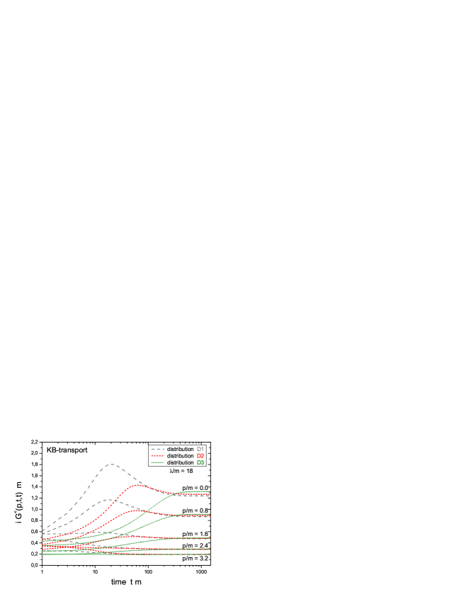
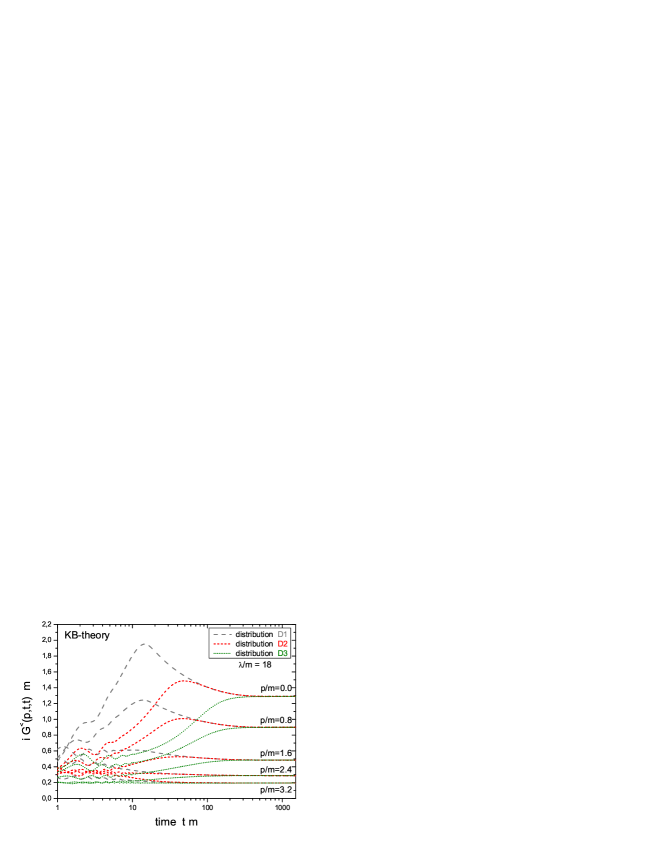
Figure 3: Upper part: Evolution of several momentum modes $|\,\vec{p}\,|/m=$ 0.0, 0.8, 1.6, 2.4, 3.2, 4.0 of the equal-time Green function on a logarithmic time scale for the different initializations D1, D2 and D3 for the generalized transport equation (2.2). Lower part: same as above but for the full Kadanoff-Baym equation (2.1).

The initial distribution functions for the following studies are shown in Fig. 2 for polar symmetric configurations as a function of the momentum coordinate $p_{x}$ for $p_{y}$ = 0. They are identical to those used in Ref. [51] within the full Kadanoff-Baym theory. The resulting initial equal-time Green functions – for the coupling constant $\lambda/m=18$ – are displayed in Fig. 2. By comparison with the initial Green functions of the Kadanoff-Baym calculation (c.f. lower part of Fig. 3 in Ref. [51]) we find tiny deviations in the region of small absolute momenta. This is, of course, a consequence of the large coupling constant $\lambda$ employed, which we use in order to compare to the calculations within the full quantum evolution for the same coupling strength. Since the initial states are very close to those used for the Kadanoff-Baym theory, we will also denote them as initializations D1, D2 and D3 as in Ref. [51].

The advantage of the initialization prescription introduced above is that the actual spectral function – directly obtained by $\bar{A}=i\bar{G}^{>}-i\bar{G}^{<}$ from the Green functions – complies with the one determined from the self-energies (33) in accordance with the first order gradient expansion scheme. During the nonequilibrium time evolution this correspondence is maintained since the analytic expression for the spectral function already is a solution of the generalized transport equation itself. Furthermore, the real part of the retarded Green function, that enters the peculiar second Poisson bracket on the l.h.s. in (2.2), can be taken in the first order scheme (34) which simplifies the calculations considerably.

We mention that other prescriptions are also possible for the calculation of $Re\,\bar{G}^{R}$:
1) One can determine it directly from $i\bar{G}^{\gtrless}$ by a Fourier technique similar to one used in the calculation of the self-consistent spectral functions in Appendix D of Ref. [51]. Here the real part of the retarded Green function is obtained via inverse Wigner transformation with respect to the energy, multiplication by the $\Theta$-function in relative time and transformation back to phase-space.
2) One can also use dispersion relations with the spectral function to specify $Re\,\bar{G}^{R}$.
As we have checked in our actual simulations all prescriptions lead to practically identical results.

3.2 Numerical Study of Equilibration

Now we turn to the actual solutions of the generalized transport equation in the KB form (2.2). In Fig. 3 (upper part) we show the time evolution of the equal-time Green function $iG^{<}(|\,\vec{p}\,|,t,t)$ for the polar symmetric initial states D1, D2 and D3 as specified in Fig. 2. We have displayed several momentum modes $|\,\vec{p}\,|/m=$ 0.0, 0.8, 1.6, 2.4, 3.2, 4.0 of the equal-time Green function on a logarithmic time scale. As in the full Kadanoff-Baym theory (lower part) we find that for all initializations the quantum system approaches a stationary state for $t\rightarrow\infty$, i.e. all momentum modes approach a constant.

However, the respective momentum modes of the different initializations do not achieve identical values for $t\rightarrow\infty$, as seen in particular for the low momenta $|\,\vec{p}\,|/m=$ 0.0, 0.8 in Fig. 3 (upper part). This is not surprising since the various initializations – obtained within the self-consistent scheme described above – do not correspond to exactly the same energy. This is why the respective long-time limits differ slightly. The small difference in energy is, of course, most prominently seen in the low momentum (energy) modes. Moreover, the dynamics within the generalized transport equation (2.2) is in general very similar to the full Kadanoff-Baym theory (lower part). For all three initial states we find (apart from the very initial phase $t\cdot m<$ 5) the same structures during the equilibration process. In particular for the initializations D1 and D2 the characteristic overshooting for the low momentum modes is seen as in the full quantum evolution, which does not show up in solutions of the corresponding on-shell Boltzmann limit. Since in the Boltzmann limit a strictly monotonous evolution of the momentum modes is seen (cf. Ref. [51]) this overshooting has to be attributed to an off-shell quantum effect. Even the positions of the maxima are in a comparable range: For the initialization D1 they are shifted to slightly larger times and are a little bit lower than in the full calculation; the same holds for the initial state D2. The initial distribution D3 yields a monotonous behaviour for all momentum modes within the generalized transport formulation which is again in a good agreement with the full dynamics.

Some comments are worthwhile with respect to the comparison performed above: The spectral function in the Kadanoff-Baym calculation is completely undetermined in the initial state; it develops during the very early phase to an approximate form (which in the following still evolves in time). In contrast to this, the spectral function in the generalized transport formulation (2.2) has a well-defined structure already from the beginning. This principle difference results from the fact, that in the Kadanoff-Baym case we deal with a true initial value problem in the two time directions ($t_{1},t_{2}$). Moreover, the spectral distribution for very early times depends on the specific initial conditions adopted (cf. Appendix C of Ref. [51]). Additionally, the relative time integral in ($t_{1}-t_{2}$) – to obtain the spectral function in energy $p_{0}$ by Wigner transformation – is very small in the initial phase as discussed in Ref. [51]. Consequently, the spectral shape in Wigner space is determined by the finite integration interval in time rather than by the interactions itself. On the other hand, we have used an infinite relative time range in deriving the generalized transport equation within the first order gradient expansion. Thus in this case we deal with a completely resolved spectral function already at the initial time, that clearly exhibits the physics incorporated. This demonstrates why both approaches can only be compared to a certain extent for the very early times.

Nevertheless, the inclusion of the dynamical spectral function in terms of the generalized transport equation surpasses the shortcomings of the quasiparticle Boltzmann limit discussed in Section V and Appendix E of Ref. [51]. Whereas the latter approach leads to a strictly monotonous evolution of the momentum modes, the inclusion of quantum effects in terms of a semiclassical approximation correctly yields the overshooting effects as in the solution of the full Kadanoff-Baym equation.

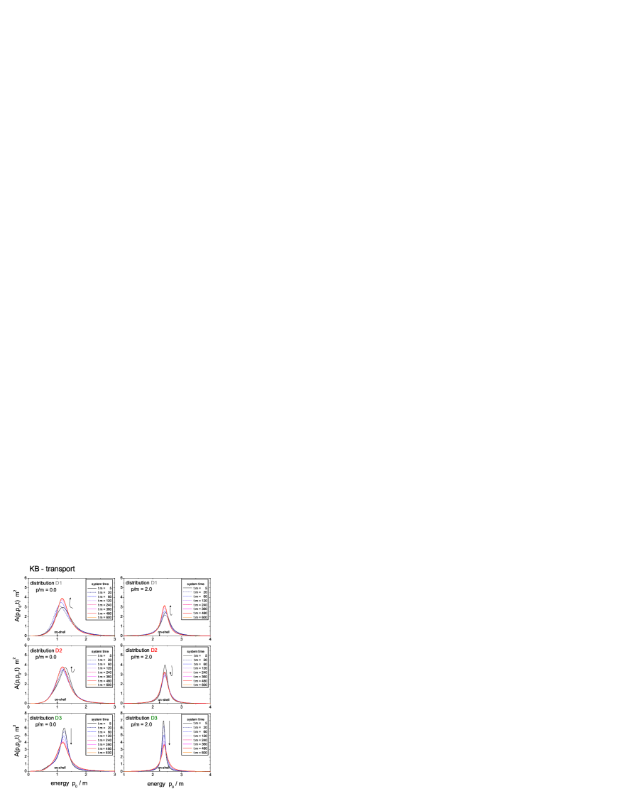
Figure 4: Time evolution of the spectral function $\bar{A}(\vec{p},p_{0},t)$ for the initial distributions D1, D2 and D3 (from top to bottom) with coupling constant $\lambda/m=$ 18 for the two momentum modes $|\,\vec{p}\,|/m=$ 0.0 (l.h.s.) and $|\,\vec{p}\,|/m=$ 0.0 (r.h.s.). The spectral function from the transport eq. (2.2) is shown for times $t\cdot m=$ 5, 20, 60, 120, 240, 360, 480, 600 as indicated by the different line types.

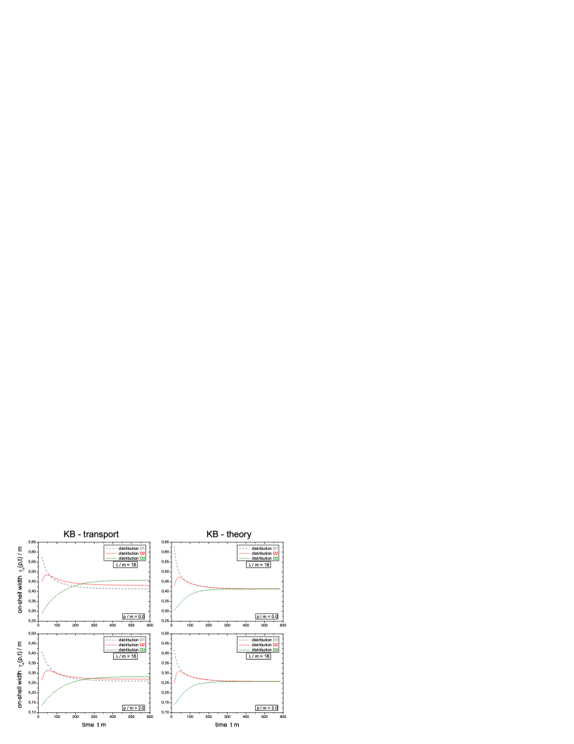
Figure 6: Time evolution of the on-shell widths $-Im\,\bar{\Sigma}^{R}(\vec{p},\omega(\vec{p},t),t)/\omega(\vec{p},t)$ of the momentum modes $|\,\vec{p}\,|/m=0.0$ and $|\,\vec{p}\,|/m=2.0$ for the different initializations D1, D2 and D3 with $\lambda/m=18$ in the semiclassical transport eq. (2.2) (l.h.s.). The respective results from the full Kadanof-Baym theory are displayed on the r.h.s.

Finally, concentrating on the very early time behaviour, we find a significant difference between the full and the approximate dynamics in the gradient scheme (2.2). For the generalized transport equation we find a monotonous evolution of the equal-time Green function momentum modes, whereas strong oscillations are observed in the initial phase for the solution of the full Kadanoff-Baym theory (see also Fig. 4 of Ref. [51]). Thus, with respect to the early time behaviour the generalized transport equation behaves much more like the Boltzmann approximation, which is a first order differential equation in time as well. However, the Kadanoff-Baym evolution is given by an integro-differential equation of second order in time. In this case the phase correlations between the Green functions $G^{<}_{\phi\phi},\,G^{<}_{\pi\phi},\,G^{<}_{\pi\pi}$ are kept and the instantaneous switching-on of the interaction results in an oscillatory behaviour of the single momentum modes. We mention that correlations build up very rapidly in the very early phase of the evolution in the full KB theory (cf. Fig. 6 of Ref. [51]) that may be attributed to this oscillatory behaviour. When including the collisional self-energies, i.e. on the three-loop level for the effective action, these oscillations are damped in time typically with the respective on-shell width for given momentum. If only the tadpole term is included, these oscillations are not damped and maintain forever (see also Fig. 4 of Ref. [51]). Therefore, the origin of the oscillatory behaviour can be traced back to the order of the underlying differential equation and the rapid build-up of correlations that have not been incorporated in the initial conditions for the full KB-theory.

3.3 Evolution of the Spectral Function

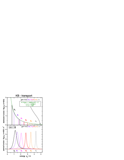
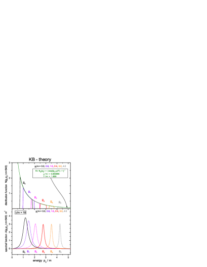
Figure 7: Spectral function $\bar{A}$ for various momentum modes as a function of energy $p_{0}/m$ at the late time $t\cdot m=$ 600 (lower part) for initial distribution D2 with coupling constant $\lambda/m=18$ in the semiclassical transport limit (2.2) (l.h.s.). The corresponding distribution function $\bar{N}$ (at the same time for the same momentum modes) is shown in the upper part. All momentum modes can be fitted for all energies by a single Bose function of temperature $T/m=$ 1.827 and a chemical potential $\mu/m$ close to zero. The respective results from the full Kadanof-Baym theory are displayed on the r.h.s.

Since the Green functions develop in time also the spectral properties of the system change as well. In Fig. 4 the time evolution of the spectral functions for the initializations D1, D2 and D3 within the gradient scheme are displayed. We focus on the spectral functions for two particular momentum modes $|\,\vec{p}\,|/m=$ 0.0 (l.h.s.) and $|\,\vec{p}\,|/m=$ 2.0 (r.h.s.) for various system times $t\cdot m=$ 5, 20, 60, 120, 240, 360, 480, 600 up to the long-time limit. This representation corresponds to Fig. 7 in Ref. [51], where the respective evolution of the spectral function is studied for the full Kadanoff-Baym theory. We find that the time evolution of the spectral functions obtained from the generalized transport equation (2.2) is very similar to the one from the full quantum calculation (see below). The zero-mode spectral function for the initial distribution D1 becomes sharper with time and is moving to slightly higher energies. The opposite characteristics is observed for the zero-mode spectral function for the initialization D3, which broadens with time (reducing the peak correspondingly) and slowly shifts to smaller energies. Together with the weak evolution for the distribution D2 (which only slightly broadens at intermediate times and returns to a narrower shape at smaller energies in the long-time limit) the evolution of all three initializations in the semiclassical approximation is well comparable to the full Kadanoff-Baym dynamics (cf. Fig. 7 in Ref. [51]). Furthermore, the maxima of the zero-mode spectral functions are located above the bare mass (as indicated by the on-shell arrow) for all initial states during the time evolution.

The spectral functions for the momentum mode $|\,\vec{p}\,|/m=$ 2.0 are in a good agreement with the Kadanoff-Baym dynamics as well. Again we observe – for the initial distribution D1 – a narrowing of the spectral function, while for D3 the spectral function broadens with time. Moreover, the width of the spectral function starting from distribution D2 shows a non-monotonous behaviour with a maximum at intermediate times.

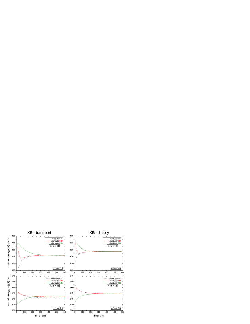
Figure 5: Time evolution of the on-shell energies $\omega(\vec{p},t)$ of the momentum modes $|\,\vec{p}\,|/m=0.0$ and $|\,\vec{p}\,|/m=2.0$ for the different initializations D1, D2 and D3 with $\lambda/m=18$ in the semiclassical KB limit (2.2) (l.h.s.). The on-shell self-energies are extracted from the maxima of the time-dependent spectral functions. The respective results from the full Kadanof-Baym theory are displayed on the r.h.s.

In order to study the dynamics of the spectral function in a more quantitative manner we display in Fig. 5 the time evolution of the on-shell energies (as derived from the maxima of the spectral function) for the momentum modes $|\,\vec{p}\,|/m=$ 0.0 (upper plot) and 2.0 (lower plot) for the initializations D1, D2 and D3 with $\lambda/m=$ 18 (l.h.s.). By comparison with the corresponding results from the Kadanoff-Baym theory (r.h.s.) we observe a close similarity of the evolutions within the full and the semiclassical KB scheme. The effective mass of the zero momentum mode decreases for initialization D3, passes a minimum for D2 and increases for the initial state D1.

As familiar from the Kadanoff-Baym calculations in Section IV.B of [51] the behaviour of the on-shell energies is different for higher momentum modes. We find for the momentum mode $|\,\vec{p}\,|/m=$ 2.0 a monotonous decrease of the on-shell energy for the initializations D1 and D2 and an increase for distribution D3. Altogether, the evolution of the on-shell energies for the higher modes is rather moderate compared to the lower ones in accordance with the dominant momentum contribution and the weakening of the retarded self-energy for higher energy modes.

Finally, the on-shell energies approach a stationary state for all modes and all initializations. However, the long-time limit of the equal momentum modes is not exactly the same for all initial distributions D1, D2 and D3. As discussed above this small difference can be traced back to the specific initial state generation from the given momentum distribution.

Next we consider the time evolution of the on-shell width as determined by the imaginary part of the retarded self-energy at the maximum position of the spectral function. In Fig. 6 (l.h.s.) the on-shell width is displayed for the two momentum modes $|\,\vec{p}\,|/m=$ 0.0 and $|\,\vec{p}\,|/m=$ 2.0 for all three initial distributions D1, D2 and D3 with $\lambda/m=$18 as a function of time. For both momentum modes the on-shell width increases for the distribution D3, while it has a maximum at intermediate times ($t\cdot m\approx$ 40) for the initialization D2. Thus the results – together with the reduction of the on-shell width for both momentum modes for the initialization D1 – is in good agreement with the results obtained for the full Kadanoff-Baym theory (r.h.s.). However, the stationary values for the on-shell widths deviate again slightly in accordance with the different preparation of the initial state in the gradient scheme.

In summarizing we find that the main characteristics of the full quantum evolution of the spectral function are maintained in the semiclassical transport equation (2.2) as well. This includes the evolution of the on-shell energies as well as the width of the spectral function. Since the generalized transport equation is formulated directly in Wigner space one has access to the spectral properties at all times, whereas the very early times in the Kadanoff-Baym case have to be excluded due to the very limited support in the relative time interval ($t_{1}-t_{2}$) for the Wigner transformation.

3.4 Stationary State of the Semiclassical Evolution

As we have observed in the previous Subsections the evolution within the generalized transport equation (2.2) leads to a stationary state for all three different initializations D1, D2 and D3. Thus we turn to the investigation of this long-time limit itself, here in particular for the initialization D2. In Fig. 7 (l.h.s.) we show the distribution function $\bar{N}$ of various momentum modes $|\,\vec{p}\,|/m=$ 0.0, 0.8, 1.6, 2.4, 3.2, 4.0 for large times ($t\cdot m$ = 600) as derived from the Green function itself and the spectral function via the relation $\bar{N}=i\bar{G}^{<}/\bar{A}$. The distribution function for a given momentum mode is calculated for all energies $p_{0}$ where the corresponding spectral function – as displayed in the lower part of Fig. 7 – exceeds a value of 0.5. Since the width of the late time spectral function decreases with increasing momentum, the energy range for which the distribution function is shown, is smaller for larger momentum modes. We find, that all momentum modes of $\bar{N}$ can be fitted at all energies by a single Bose function with a temperature $T/m=$ 1.827 and a very small chemical potential $\mu/m=$ 0.000817. Thus the generalized transport formulation (2.2) leads to a complete (off-shell) equilibration of the system very similar to the solution of the full Kadanoff-Baym equation (r.h.s. of Fig. 7). Furthermore, the long-time limit of the semiclassical time evolution exhibits a vanishing chemical potential $\mu/m$ in accordance with the properties of the neutral $\phi^{4}$-theory. This might have been expected since in the generalized transport equation particle number non-conserving processes of the type $1\leftrightarrow 3$ – which lead to the decrease of the chemical potential – are included by means of the dynamical spectral function. Thus the semiclassical approximation (2.2) solves the problems within the Boltzmann limit, which does not yield a relaxation of the chemical potential, since only on-shell $2\leftrightarrow 2$ transitions of quasiparticles are taken into account as demonstrated in Section V of Ref. [51].

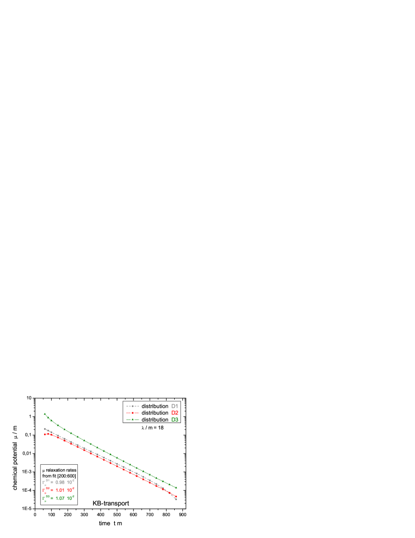
Figure 8: Relaxation of the chemical potential $\mu/m$ for the three initial distributions D1, D2, D3 within the generalized transport equation (2.2) in a logarithmic repesentation as a function of time. The decrease is approximately exponential in time $\propto\exp(-\Gamma_{\mu}\cdot t)$ and the relaxation rate $\Gamma_{\mu}$ is practically equal for all initializations.

After observing, that the chemical potential decreases to zero in the long-time limit, it is interesting to study the relaxation process itself. The relaxation of the chemical potential $\mu/m$ is shown for the three different initializations D1, D2 and D3 with coupling constant $\lambda/m=$ 18 in Fig. 8. We see – as in the case of the Kadanoff-Baym evolution – that all initial states show an approximately exponential decrease in time. The relaxation rates – as determined from the slope of the exponential decline – are also approximately the same for all distributions. They are given by $\Gamma^{D1}_{\mu}\approx 0.98\cdot 10^{-2}$ for distribution D1, $\Gamma^{D2}_{\mu}\approx 1.01\cdot 10^{-2}$ for distribution D2 and $\Gamma^{D3}_{\mu}\approx 1.07\cdot 10^{-2}$ for distribution D3. Thus the relaxation rates are in the same range as those found within the full Kadanoff-Baym theory (Section IV.D in Ref. [51]). This is exactly the result one expects from the analytical estimate for the chemical potential relaxation rate. In Section IV.D of Ref. [51] we have found that the relaxation rate $\Gamma_{\mu}$ can be explained within a linearized evolution equation including only equilibrium properties, i.e. the equilibrium spectral and (Bose) distribution function. It is appropriate for small deviations from the equilibrium state in terms of the chemical potential $\mu$. In the present case of the generalized transport equation (2.2) we encounter exactly the same situation. We know from the validity of the estimate that a linearized description is meaningful. Thus the evolution within the first order gradient equation should yield a comparable result as long as the equilibrium properties are about equal. This is indeed the case since the final temperatures for the various initial states are approximately the same (also compared to the Kadanoff-Baym case). They are given by $T^{D1}_{eq}/m\approx 1.819$, $T^{D2}_{eq}/m\approx 1.827$, $T^{D3}_{eq}/m\approx 1.834$ compared to $T_{eq}/m\approx 1.835$ in the full Kadanoff-Baym case. Consequently, the same similarity holds for the spectral function, which is determined in equilibrium by the temperature $T$ and the coupling strength $\lambda$. Therefore we can conclude, that the generalized transport equation (2.2) is sufficient to describe the correct relaxation of the chemical potential $\mu$.

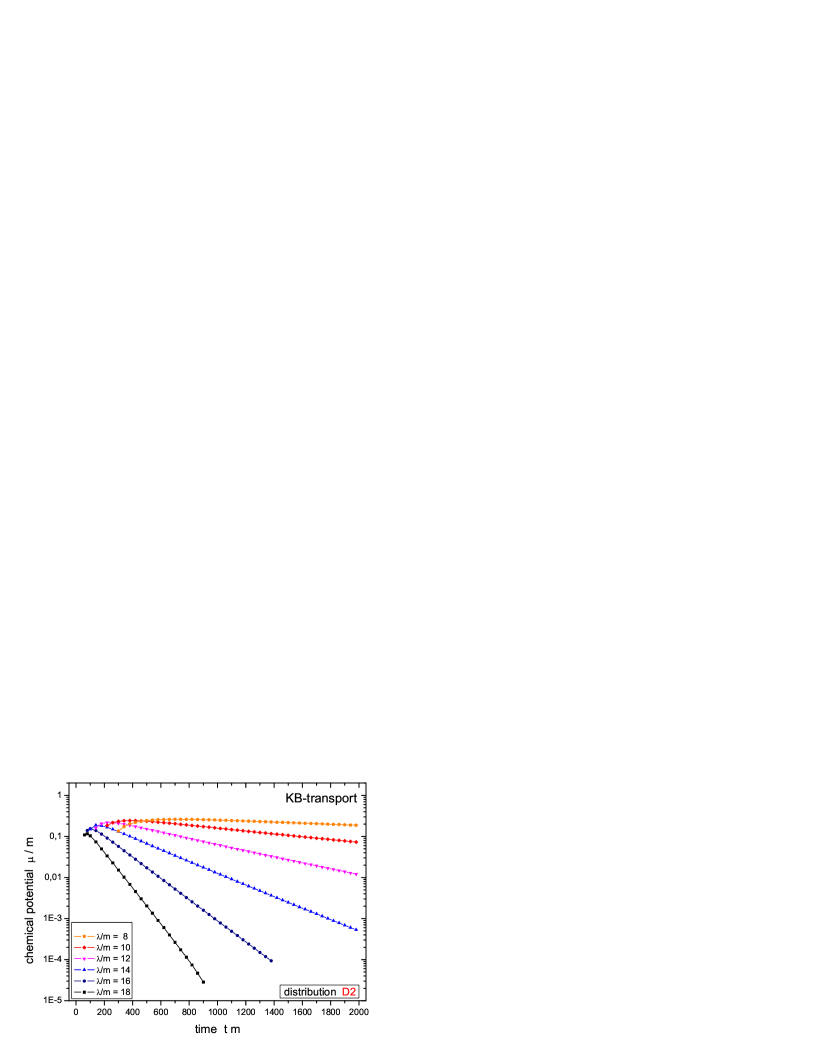
Figure 9: Relaxation of the chemical potential $\mu/m$ for initial distribution D2 with coupling constants $\lambda/m=$ 8, 10, 12, 14, 16, 18 using the generalized transport equation (2.2).

Finally, we study the relaxation of the chemical potential as a function of the coupling strength $\lambda$. To this aim we display in Fig. 9 the relaxation of the chemical potential $\mu$ for the initial distribution D2 for coupling constants $\lambda/m=$ 8, 10, 12, 14, 16, 18 as obtained form the generalized transport equation (2.2). For all coupling constants $\lambda$ the chemical potential $\mu$ is reduced exponentially in time $\propto\exp(-\Gamma_{\mu}\cdot t)$ and thus allows for the determination of a proper relaxation rate $\Gamma_{\mu}$.

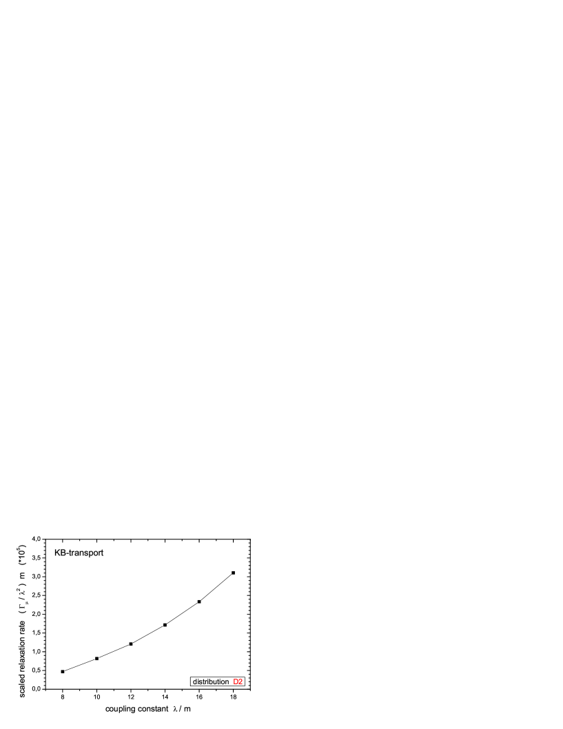
Figure 10: Scaled relaxation rate $\Gamma_{\mu}/\lambda^{2}$ of the chemical potential as a function of the coupling strength $\lambda/m$ for the initial distribution D2.

The results for the relaxation rates $\Gamma_{\mu}$ of the chemical potential as a function of the coupling strength $\lambda$ are displayed in Fig. 10. They are scaled by the coupling constant squared ($\lambda^{2}$) in order to take into account the overall coupling dependence of the collisional self-energy. We see that the relaxation rate $\Gamma_{\mu}$ increases much stronger than quadratically with the coupling strength. Whereas the relaxation is very weak for small and medium couplings $\lambda/m\leq$ 8, it increases considerably for larger interaction strength. By inspection of the analytical estimate for the relaxation rate of the chemical potential (Eq. (4.28) in Ref. [51]) we find an explanation for this strong dependence: At first here an overall factor of the coupling constant squared ($\lambda^{2}$) enters the expression for the relaxation rate, that stems from the collisional integral in terms of the scattering (sunset) self-energies. This factor, only, would yield a constant line in Fig. 10 and thus underestimate the observed behaviour significantly. Therefore, one has to keep in mind the additional $\lambda$ dependence of the (equilibrium) spectral function that strongly influences the estimate for the relaxation rate since it appears in the energy-momentum integration weights several times. Thus the relaxation rate is determined explicitly via the $K_{2}$-term (Eq. (4.26) in Ref. [51]) and implicitly through the spectral functions in both contributions, $K_{1}$ and $K_{2}$ (Eqs. (4.26) in Ref. [51]), by the coupling strength $\lambda$ in a nonlinear way.

We conclude that – though there is a small relative shift of the different time scales of kinetic and chemical equilibration as a function of the coupling strength $\lambda$ with respect to the full KB solutions – the results of the generalized transport equations are very similar. The differences we attribute to higher order multi-particle effects in off-shell transitions. While the kinetic equilibration proceeds approximately with the coupling constant squared (as indicated by the calculations for non-polar-symmetric systems), the chemical relaxation rate is a higher order process in $\lambda$ as seen from Fig. 10. Thus the chemical equilibration moves with increasing coupling strength $\lambda$ to earlier times relative to the kinetic relaxation, which is governed by terms $\sim\lambda^{2}$ (see next Subsection).

3.5 Quadrupole Relaxation

In this Section we no longer restrict to polar symmetric systems and discuss the time evolution of more general initial distributions within the generalized transport approximation (2.2). We start with conditions similar to those employed in Section V of Ref. [51], but combined with the initialization scheme for the semiclassical limit. Again – as in the full Kadanoff-Baym and the Boltzmann case (Section V of Ref. [51]) – the decrease of the quadrupole moment of the distribution

$$Q(t)\>=\>\frac{\displaystyle{\int\!\!\frac{d^{2}p}{(2\pi)^{2}}\;\;[\,p_{x}^{2}-p_{y}^{2}\,]\;\;N(\vec{p},t)}}{\displaystyle{\int\!\!\frac{d^{2}p}{(2\pi)^{2}}\;\;N(\vec{p},t)}}\;,$$ (55)

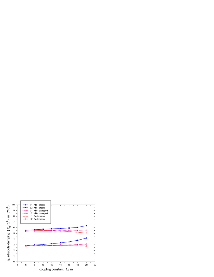
Figure 11: Scaled Relaxation rate for the generalized transport equation as a function of the coupling strength (half-filled symbols) for the initial distributions d1 (squares) and d2 (triangles). Additionally the results obtained within the Kadanoff-Baym (full symbols) and the Boltzmann calculation (open symbols) are shown for comparison.

is approximately exponential in time ($\propto\exp(-\Gamma_{Q}\cdot t)$) and thus allows for the extraction of a quadrupole damping rate $\Gamma_{Q}$. The scaled quadrupole damping rates – as obtained for the two initial distributions d1 and d2 (cf. Section V of Ref. [51]) – are displayed in Fig. 11 as a function of the coupling strength $\lambda/m$. The calculations show that the quadrupole relaxation rates within the semiclassical approximation (2.2) for both initial distributions d1 and d2 is well within in the range of the full Kadanoff-Baym and the on-shell Boltzmann case. Additionally, the quadrupole relaxation rate is rather flat in the coupling $\lambda$ when divided by the coupling constant squared ($\lambda^{2}$) as already observed for the other two evolution schemes in Section V of Ref. [51]. Nevertheless, the relaxation in the full KB-theory (2.1) proceeds slightly faster than in the transport limits for large couplings. The latter effect is again attributed to higher order off-shell transition effects which are no longer incorporated in the generalized transport equation.

3.6 Validity of the Gradient Approximation

As we have seen in the previous Subsections the generalized transport equation (2.2) leads to a good agreement with the Kadanoff-Baym dynamics. This indicates that the semiclassical limit can be applied without loosing essential features of the full quantum dynamics for homogeneous systems (in particular for the initializations D1, D2 and D3). We recall, that the underlying assumption for the validity of the first order gradient expansion scheme – which has been used to derive the generalized transport equation – is that all functions are slowly evolving in the mean space and time coordinates. Thus, in comparison to the first order time derivatives, the second order time derivatives should be small, such that they can be neglected to a good approximation. In this Subsection we will study now this criterion in a more quantitative way.

To this aim we consider as a relative measure the energy-momentum integrals over the absolute value of first and second order time derivatives of various functions entering the generalized transport equation. Explicitly this measure is given at time $t$ by

$$M^{1/2}_{F}(t)\;=\;\int\frac{d^{D}p}{(2\pi)^{D}}\;\;\left|\;\partial_{t}^{(1/2)}\;\bar{F}(\vec{p},p_{0},t)\;\right|$$ (56)

for an arbitrary function $\bar{F}$ in Wigner space. In the following we take into account the time derivatives of the Green functions and the self-energies, i.e.

$$\bar{F}\>\in\>\{\,i\bar{G}^{<},\,i\bar{\Sigma}^{<},\,Re\,\bar{G}^{R},\,Re\,\bar{\Sigma}^{R}\,\}\>.$$ (57)

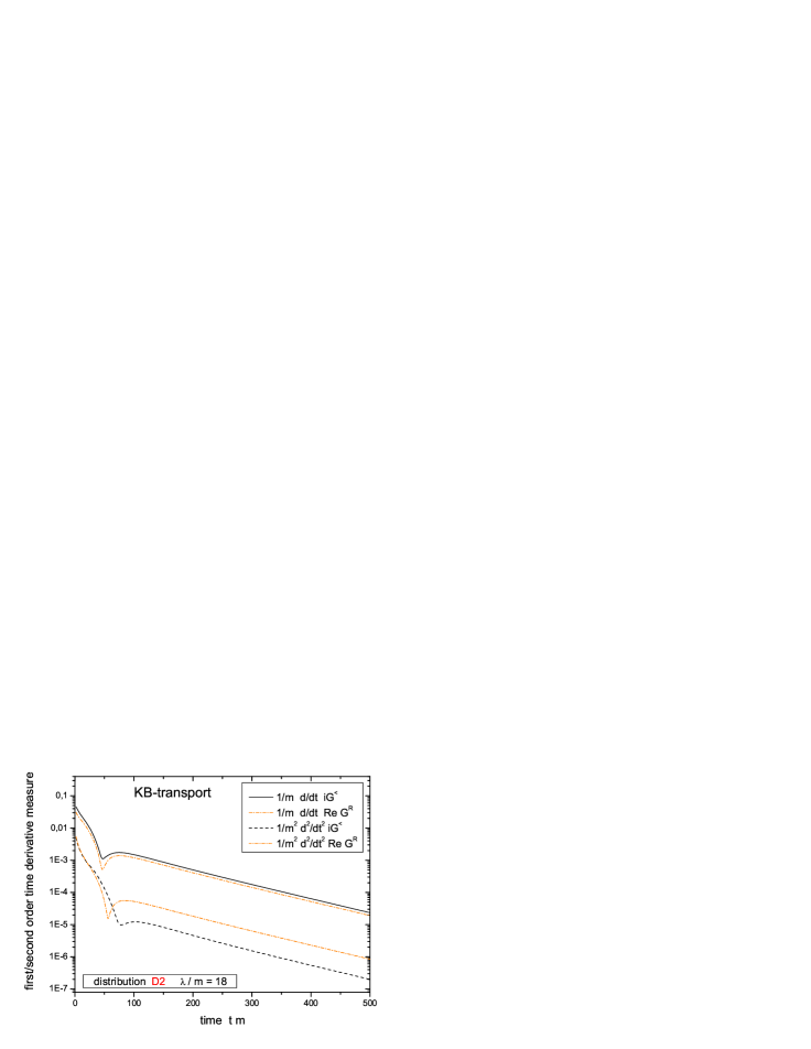
Figure 12: Time evolution of the first/second order time derivative measure for the Green functions $i\bar{G}^{<}$ and $Re\,\bar{G}^{R}$ for initial distribution D2 with coupling constant $\lambda/m=$ 18. During the whole evolution the second order time derivatives are more than an order of magnitude smaller than the first order derivatives supporting the validity of the gradient expansion. Note that time derivatives in our convention are derivatives with respect to the dimensionless quantity $tm$.

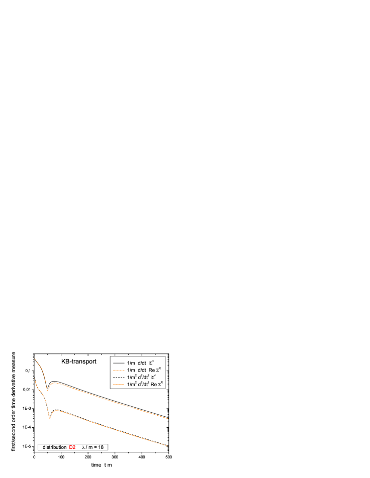
Figure 13: Time evolution of the first/second order time derivative measure for the functions $i\bar{\Sigma}^{<}$ and $Re\,\bar{\Sigma}^{R}$ for initial distribution D2 with coupling constant $\lambda/m=$ 18. During the whole evolution the second order time derivatives are significantly smaller than the first order contributions. Note that time derivatives in our convention are derivatives with respect to the dimensionless quantity $tm$.

The time evolution of these measures is shown in Fig. 12 for the first and the second order time derivatives of the Green function and in Fig. 13 for the collisional and the retarded self-energies. The calculation has been performed for the initial distribution D2 with a coupling strength of $\lambda/m=$ 18. For the Green functions as well as the self-energies the second order time derivatives are about one order of magnitude smaller than the first order expressions. Thus the underlying assumption of the first order gradient expansion is fulfilled very well indicating that the results obtained within the semiclassical scheme should match with those for the full quantum evolution to a large extent. This is exactly what we have found from the explicit comparison of the evolution of the equal-time Green functions as well as the spectral functions in Sections 3.2 and 3.3.

3.7 Generalized Transport in Botermans-Malfliet Form

In this Subection we will perform a comparison of the generalized transport equation in the original Kadanoff-Baym (KB) form (2.2) with the modified Botermans-Malfliet (BM) form (51). As discussed in detail in Section 2.2 the latter form results from the replacement of the collisional self-energy by

$$i\bar{\Sigma}^{<}\rightarrow i\bar{G}^{<}\cdot\bar{\Gamma}/\bar{A}$$ (58)

in the second Poisson bracket on the l.h.s. of the original kinetic equation (2.2). This replacement leads to a consistent first order equation in the gradients and achieves consistency of the resulting transport equation with the corresponding generalized mass-shell relation (46).

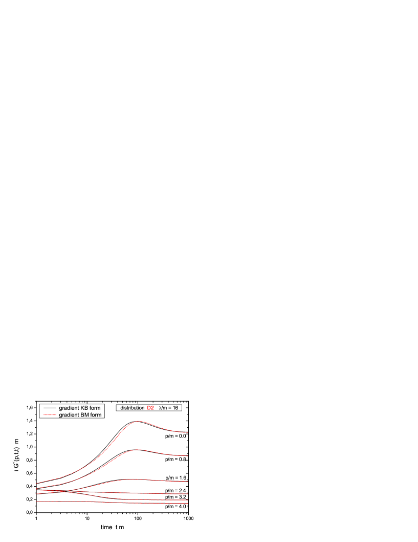
Figure 14: Time evolution of various equal-time Green function momentum modes within the generalized transport equation (original KB form, solid lines) and within the Botermans-Malfiet (BM) form (dashed lines) for initial distribution D2 with coupling constant $\lambda/m=16$.

In Fig. 14 we compare the time evolution within the generalized transport equation in the KB form to the consistent equation in BM form. In this respect several momentum modes of the equal-time Green function are displayed evolving in time from an initial distribution D2 for a coupling constant $\lambda/m=$ 16. We find that the deviations between both approximations (KB and BM) are rather moderate. Only for very small momentum modes $|\,\vec{p}\,|/m\leq$ 1.6 deviations between both calculational modes are visible. For the very low momentum modes the range of difference starts at $t\cdot m\approx$ 10 and extends to $t\cdot m\approx$ 100 for the non-zero modes. For the zero momentum mode the deviation lasts even longer. In this region the semiclassical transport in the BM form is slightly ’slower’ than in the original KB choice. Nevertheless, also the BM form exhibits the typical overshooting behaviour of the low momentum modes beyond the stationary limit as observed for the KB form. However, the maxima are shifted slightly to later times. Finally, both gradient approximations converge in the long-time limit to very similar configurations.

As the final part of the comparison we investigate the approximation (58) quantitatively and introduce a measure for the absolute strength of the collision term by integrating the collision rates over energy and momentum. Since the collision term vanishes, if the substitution (58) holds exactly, i.e. in equilibrium, the absolute size gives an idea about the validity of this replacement at the zero order level. Explicitly the measure reads:

$$M_{col}(t) = \int\!\!\frac{d^{D}p}{(2\pi)^{D}}\;\;\frac{1}{|\,2p_{0}\,|}\>\left|\;\phantom{\frac{1}{2}}\!\!i\bar{\Sigma}^{<}\;i\bar{G}^{>}\;-\;i\bar{\Sigma}^{>}\;i\bar{G}^{<}\;\right|\;.$$ (59)

Furthermore, we define a measure for the deviation of the second Poisson bracket in the original and in the consistent Botermans-Malfliet formulation. It is given by the integration over the absolute differences of the Poisson terms as

$$M_{off}(t) = \int\!\!\frac{d^{D}p}{(2\pi)^{D}}\;\;\frac{1}{|\,2p_{0}\,|}\>\left|\;\{\,i\bar{\Sigma}^{<}\,,\,Re\,\bar{G}^{R}\,\}\;-\;\{\,i\bar{G}^{<}\,\frac{\bar{\Gamma}}{\bar{A}}\,,\,Re\,\bar{G}^{R}\,\}\;\right|\;.$$ (60)

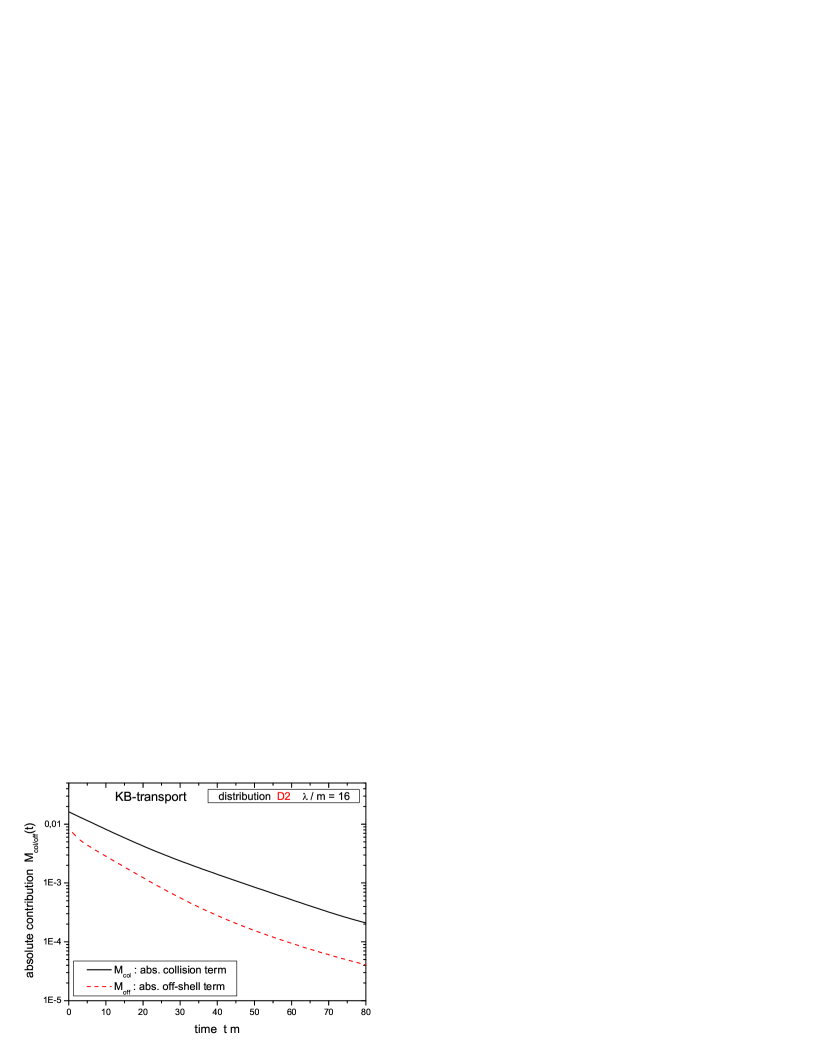
Figure 15: Time evolution of the measure functions for the collision term (59) and the difference of the second Poisson bracket in standard (KB) and consistent (BM) form (60) for the initial distribution D2 with coupling constant $\lambda/m=$ 16. Both contributions decrease in time in accordance with the equilibration of the system. The Poisson contribution (dashed line) is always significantly smaller than that of the collision term (solid line).

In Fig. 15 we display the time evolution of the measure (59) (solid line) and the measure (60) (dashed line). The calculation has been performed for the initial state D2 with a coupling constant $\lambda/m=$ 16. We find that both measures decrease as a function of time in accordance with the equilibration of the system. Additionally, the contribution from the difference of the Poisson brackets (60) is always smaller than the one stemming from the collision term (59). This indicates that the replacement of the collisional self-energy $i\bar{\Sigma}^{<}\rightarrow i\bar{G}^{<}\cdot\bar{\Gamma}/\bar{A}$ is more reliable when it takes place at the gradient level in accordance with the assumption of Botermans and Malfliet. However, the relative suppression is not very large.

In summary we point out that the approximation of the full Kadanoff-Baym dynamics by the generalized transport equations in Kadanoff-Baym (2.2) or Botermans-Malfliet form (51) holds very well for the different momentum modes of the Green function $i\bar{G}^{<}$ itself. Slight deviations are only visible for the zero momentum mode at early to intermediate times (Figs. 3 and 14) for a logarithmic representation of the time axis. Consequently, the characteristic features of quantum equilibration obtained for the full Kadanoff-Baym theory are retained in the generalized transport limits. The validity of these transport equations – based on a first order gradient expansion – could be shown explicitly, since second order gradient terms turned out to be smaller by more than an order of magnitude (cf. Figs. 12 and 13).

4 Summary and Outlook

In this work we have studied the quantum time evolution of $\phi^{4}$-field theory for homogeneous systems in 2+1 space-time dimensions for far-from-equilibrium initial conditions in extension of our studies in Ref. [51]. The three-loop approximation for the CTP 2PI effective action has been employed, i.e. the tadpole and sunset self-energies. The tadpole contribution corresponds to a dynamical mass term whereas the sunset self-energy is responsible for dissipation and an equilibration of the system. Since both self-energies are ultraviolet divergent, they had to be renormalized by including proper counter terms. The numerical solutions for different initial configurations out of equilibrium (with the same energy density) show, that the asymptotic state achieved for $t\rightarrow\infty$ is the same for all initial conditions in the full Kadanoff-Baym theory.

In order to improve the standard on-shell (or quasiparticle) Boltzmann transport theory we have derived generalized off-shell transport equations from the Kadanoff-Baym equations in phase-space representation by restricting to first order derivatives in $x$ and $p$. In fact, it could been shown explicitly, that second order derivatives (of self-energies and Green functions) are smaller than the first order derivatives by at least an order of magnitude. As a consequence the dynamics within the generalized transport formulation shows a very similar structure as the full quantum solution. This is clearly seen for the propagation of the equal-time momentum modes of the Green functions and the evolution of the spectral function for all configurations considered. It includes, in particular, the overshooting behaviour of the low momentum equal-time modes, which occurs at intermediate times depending on the initial distribution. Furthermore, the evolution within the generalized transport equation leads to a stationary state in the long time limit, which exhibits a full off-shell equilibration with vanishing chemical potential. Even the relaxation rates of the chemical potential obtained from the semiclassical evolution agree very well with those of the full Kadanoff-Baym theory. The dependence of the chemical relaxation rate on the coupling constant is rather non-trivial, since it is strongly affected by the equilibrium spectral function. Thus we conclude that the inclusion of the dynamical spectral function – as inherent in the semiclassical approximation of the KB equations – surpasses the shortcomings of the on-shell Boltzmann limit.

Moreover, we have shown that the generalized transport equation in Kadanoff-Baym (KB) form (2.2) and in Botermans-Malfliet (BM) form (51) lead to comparable results for the time evolution of the initial configurations considered. Only for the time-dependent occupation of low momentum modes slight differences have been observed. This is a typical quantum phenomenon related to the large de Broglie wavelength of the low momentum modes. We stress that the generalized transport equation in BM form can be used for the off-shell description of realistic heavy-ion collisions [2, 3, 40, 41] – as well as many other interacting systems in various fields of physics – since it allows for an economic solution within an extended testparticle ansatz.

Coming back to the questions raised in the Introduction, we have to answer the first one by ’probably no’ since off-shell quantum transitions in comparison to on-shell two-body scattering only lead to slightly smaller relaxation times e.g. for the quadrupole moment in momentum space. On the other hand, the off-shell transitions are important (in case of the $\phi^{4}$-theory) for chemical equilibration, which essentially proceeds via $1\leftrightarrow 3$ transitions [51]. The latter are forbidden in the on-shell quasiparticle limit due to energy and momentum conservation. We recall that also $0\leftrightarrow 4$ processes are incorporated in the full Kadanoff-Baym theory though their effect was found to be very limited for the dynamical configurations investigated here.

Nevertheless, this still leaves us with the open question on the relative importance of many-body scattering processes $n\leftrightarrow m$ for $n\geq 2,m>2$. Here, an appropriate formulation of $n\leftrightarrow m$ off-shell and on-shell scattering processes has already been given in Ref. [59] as well as an application to the problem of antibaryon annihilation and recreation by several mesons in relativistic nucleus-nucleus collisions. A related study on the problem of $2\leftrightarrow 3$ transitions (e.g. bremsstrahlung for massless particles) on the parton level will be presented in the near future [60].

References

- [1] D. Molnar and M. Gyulassy, Nucl. Phys. A 697 (2002) 495; A 703 (2002) 893.
- [2] W. Cassing and S. Juchem, Nucl. Phys. A 665 (2000) 377.
- [3] W. Cassing and S. Juchem, Nucl. Phys. A 672 (2000) 417.
- [4] J. Schwinger, J. Math. Phys. 2 (1961) 407.
- [5] P. M. Bakshi and K. T. Mahanthappa, J. Math. Phys. 4 (1963) 1, 12.
- [6] L. V. Keldysh, Zh. Eks. Teor. Fiz. 47 (1964) 1515; Sov. Phys. JETP 20 (1965) 1018.
- [7] R. A. Craig, J. Math. Phys. 9 (1968) 605.
- [8] K. Chou, Z. Su, B. Hao, and L. Yu, Phys. Rept. 118 (1985) 1.
- [9] L. P. Kadanoff and G. Baym, Quantum statistical mechanics, Benjamin, New York, 1962.
- [10] D. F. DuBois in Lectures in Theoretical Physics, edited by W. E. Brittin (Gordon and Breach, NY 1967), pp 469-619.
- [11] P. Danielewicz, Ann. Phys. (N.Y.) 152 (1984) 239.
- [12] E. Calzetta and B. L. Hu, Phys. Rev. D 37 (1988) 2878.
- [13] H. Haug and A. P. Jauho, Quantum Kinetics in Transport and Optics of Semiconductors, Springer, New York, 1999.
- [14] C. Greiner and S. Leupold, Ann. Phys. 270 (1998) 328.
- [15] W. Cassing, Z. Physik A 327 (1987) 447.
- [16] W. Cassing, K. Niita, and S. J. Wang, Z. Physik A 331 (1988) 439.
- [17] W. Cassing, V. Metag, U. Mosel, and K. Niita, Phys. Rept. 188 (1990) 363.
- [18] W. Cassing and U. Mosel, Prog. Part. Nucl. Phys. 25 (1990) 235.
- [19] B. Bezzerides and D. F. DuBois, Ann. Phys. 70 (1972) 10.
- [20] P. Lipavský, V. Špička, and B. Velický, Phys. Rev. B 34 (1986) 6933.
- [21] V. Špička and P. Lipavský, Phys. Rev. Lett. 73 (1994) 3439; Phys. Rev. B 52 (1995) 14615.
- [22] W. Botermans and R. Malfliet, Phys. Rept. 198 (1990) 115.
- [23] S. Mrówczyński and P. Danielewicz, Nucl. Phys. B 342 (1990) 345.
- [24] A. Makhlin, Phys. Rev. C 52 (1995) 995; A. Makhlin and E. Surdutovich, Phys. Rev. C 58 (1998) 389.
- [25] K. Geiger, Phys. Rev. D 54 (1996) 949; Phys. Rev. D 56 (1997) 2665.
- [26] D. A. Brown and P. Danielewicz, Phys. Rev. D 58 (1998) 094003.
- [27] J. P. Blaizot and E. Iancu, Nucl. Phys. B 557 (1999) 183.
- [28] Y. B. Ivanov, J. Knoll, and D. N. Voskresensky, Nucl. Phys. A 657 (1999) 413.
- [29] J. Knoll, Y. B. Ivanov, and D. N. Voskresensky, Ann. Phys. 293 (2001) 126.
- [30] C. de Dominicis and P. Martin, J. Math. Phys. 5 (1964) 14.
- [31] J. M. Cornwall, R. Jackiw, and E. Tomboulis, Phys. Rev. D 10 (1974) 2428.
- [32] Gy. Wolf, W. Cassing, and U. Mosel, Nucl. Phys. A552 (1993) 549
- [33] R. Rapp and J. Wambach, Adv. Nucl. Phys. 25 (2000) 1.
- [34] W. Cassing and E. L. Bratkovskaya, Phys. Rept. 308 (1999) 65.
- [35] P. A. Henning, Phys. Rept. 253 (1995) 235; Nucl. Phys. A 582 (1995) 633.
- [36] Y. B. Ivanov, J. Knoll, and D. N. Voskresensky, Nucl. Phys. A 672 (2000) 313.
- [37] Y. B. Ivanov, J. Knoll, and D. N. Voskresensky, Phys. Atom. Nucl. 66 (2003) 1902.
- [38] S. Leupold, Nucl. Phys. A 672 (2000) 475; Nucl. Phys. A 695 (2001) 377.
- [39] M. Effenberger, E. L. Bratkovskaya, and U. Mosel, Phys. Rev. C 60 (1999) 044614; M. Effenberger and U. Mosel, Phys. Rev. C 60 (1999) 051901.
- [40] W. Cassing and S. Juchem, Nucl. Phys. A 677 (2000) 445.
- [41] W. Cassing, L. Tolos, E. L. Bratkovskaya, and A. Ramos, Nucl. Phys. A 727 (2003) 59.
- [42] P. Danielewicz, Ann. Phys. (N.Y.) 152 (1984) 305.
- [43] C. Greiner, K. Wagner, and P.-G. Reinhard, Phys. Rev. C 49 (1994) 1693.
- [44] H. S. Köhler, Phys. Rev. C 51 (1995) 3232.
- [45] H. S. Köhler and K. Morawetz, Eur. Phys. J. A 4 (1999) 291; Phys. Rev. C 64 (2001) 024613.
- [46] A. Wackert, A. Jauho, S. Rott, A. Markus, P. Binder, and G. Döhler, Phys. Rev. Lett. 83 (1999) 836.
- [47] K. Morawetz, Nonequilibrium at short time scales – Formation of correlations, Springer, Berlin, 2003.
- [48] H. van Hees and J. Knoll, Phys. Rev. D 65 (2002) 025010.
- [49] H. van Hees and J. Knoll, Phys. Rev. D 65 (2002) 105005.
- [50] J.-P. Blaizot, E. Iancu and U. Reinosa, hep-ph/0312084.
- [51] S. Juchem, W. Cassing, and C. Greiner, arXiv:hep-ph/0307353, Phys. Rev. D, in press.
- [52] J. M. Häuser, W. Cassing, A. Peter, and M. H. Thoma, Z. Phys. A 353 (1995) 301.
- [53] A. Peter, W. Cassing, J. M. Häuser, and M. H. Thoma, Z. Phys. C 71 (1996) 515; Z. Phys. A 358 (1997) 91.
- [54] J. Berges and J. Cox, Phys. Lett. B 517 (2001) 369.
- [55] G. Aarts and J. Berges, Phys. Rev. D 64 (2001) 105010.
- [56] J. Berges, Nucl. Phys. A 699 (2002) 847.
- [57] J. M. Luttinger and J. C. Ward, Phys. Rev. 118 (1960) 1417.
- [58] G. Baym, Phys. Rev. 127 (1962) 1391.
- [59] W. Cassing, Nucl. Phys. A700 (2002) 618.
- [60] Z. Xu and C. Greiner, to be published.