Fermionic Squeezed State for Simple Algebraic Models in Many-Fermion Systems

1 Introduction

As a possible extension of the time-dependent Hartree-Fock (TDHF) theory, a quasi-spin squeezed state was introduced instead of the Slater determinantal state as a possible extension of the trial state of variation.[1, 2] This state realizes the minimum uncertainty relation as well as the Slater determinantal state as a certain kind of coherent state. However, contrary with the coherent state approach, the quasi-spin squeezed state approach can take account of degrees of freedom for quantum fluctuations dynamically. Hereby, the squeezed state approach gives the better approximation than the coherent state approach in general.

In the preceding work,[1, 2] applications of the quasi-spin squeezed state for many-fermion systems carried out in simple algebraic models. For example, the application to the Lipkin model[3] where the particle-hole interaction is active shows clearly that the quasi-spin squeezed state gives the useful and powerful approximation,[2] because quantum fluctuations are contained properly. In this model, the quasi-spin squeezed state was constructed so as to take account of the particle-hole correlation. We call here it the particle-hole type squeezed state. This state reproduced the phase transition neatly, and in a certain limiting case for this state, the RPA equation was recaptured.[4, 5] From this viewpoint, the variational method with the quasi-spin squeezed state surpasses the RPA for many-fermion systems.

This paper is devoted to the purpose of the application and promotion of the quasi-spin squeezed state to the models with pairing interaction. One of the present authors (Y.T.) with Yamamura and Kuriyama have given a way to construct the quasi-spin squeezed state for pairing model.[1] Also, two of the present authors (H.A. and Y.T.) have given a possible treatment of the degree of freedom for the quantum fluctuations in the Lipkin model.[6] In this paper, we extend the treatment previously given[6] to the dynamical treatment in the pairing model. In the pairing model, we investigate the ground state energy with two different manners using the quasi-spin squeezed state. One is that the quasi-spin squeezed state is used in the framework of the time-dependent variational principle, and the system is considered dynamically. The other is that the energy minimum is sought directly introducing the chemical potential for the particle number conservation.

Further, we extend the quasi-spin squeezed state for the pairing model to the O(4) model. Recently, to investigate the shape coexistence phenomena of nucleus, the simplest $O(4)$ algebraic model with the pairing and the quadrapole interactions has been reanalyzed beyond the Hartree-Fock-Bogoliubov and the random phase approximations.[7, 8] As an extension of the paring type quasi-spin squeezed state, we attempt to construct possible quasi-spin squeezed states for the $O(4)$ model.

This paper is organized as follows. In the next section, the exact treatment and the Hartree-Fock approximation of pairing model[9, 10, 11] are recapitulated containing notation. In §3, the time-dependent variational approach with the quasi-spin squeezed state for the pairing model is formulated. Also, it is shown that the ground state energy is well reproduced analytically in this dynamical approach. Against the former section, in §4, a static treatment, that is, the variation for the Hamiltonian with the chemical potential for the particle number conservation is carried out, and the ground state energy is estimated numerically in the pairing model. In §5, the extensions of the pairing-type squeezed state to the one for the $O(4)$ model are given. The energy expectation value for the ground state is calculated numerically by using two candidates of the squeezed states for the $O(4)$ model. The expectation values for the various operators with respect to two squeezed states are summarized in Appendix A and B, respectively. The last section is devoted to a summary.

2 Recapitulation of exact solution and coherent state approximation for pairing model with single energy level

In this section, the exact treatment of an exactly solvable quantum many-fermion model, which is called the pairing model, is reviewed for later convenience. Also, the coherent state approximation, which corresponds to the BCS approximation, is recapitulated.

2.1 Exact solution for the pairing model

We investigate a simple many-fermion system in which there exists $N$ identical fermions in a single spherical orbit with pairing interaction. The single particle state is specified by a set of quantum number $(j,m)$, where $j$ and $m$ represent the magnitude of angular momentum of the single particle state and its projection to the $z$-axis, respectively. Thus, let us start with the following Hamiltonian :

$${\hat{H}}=\epsilon\sum_{m}{\hat{c}}^{\dagger}_{m}{\hat{c}}_{m}-\frac{G}{4}\sum_{m}(-)^{j-m}{\hat{c}}_{m}^{\dagger}{\hat{c}}_{-m}^{\dagger}\sum_{m}(-)^{j-m}{\hat{c}}_{-m}{\hat{c}}_{m}\ ,$$ (2.1)

where $\epsilon$ and $G$ represent the single particle energy and the force strength, respectively. The operators ${\hat{c}}_{m}$ and ${\hat{c}}_{m}^{\dagger}$ are the fermion annihilation and creation operators with the quantum number $m$, which obey the anti-commutation relations :

$$\{\ {\hat{c}}_{m}\ ,\ {\hat{c}}_{m^{\prime}}^{\dagger}\ \}=\delta_{mm^{\prime}}\ ,\qquad\{\ {\hat{c}}_{m}\ ,\ {\hat{c}}_{m^{\prime}}\ \}=\{\ {\hat{c}}_{m}^{\dagger}\ ,\ {\hat{c}}_{m^{\prime}}^{\dagger}\ \}=0\ .$$ (2.2)

We introduce the following operators :

$${\hat{S}}_{+}=\frac{1}{2}\sum_{m}(-)^{j-m}{\hat{c}}_{m}^{\dagger}{\hat{c}}_{-m}^{\dagger}\ ,\quad{\hat{S}}_{-}=\frac{1}{2}\sum_{m}(-)^{j-m}{\hat{c}}_{-m}{\hat{c}}_{m}\ ,\quad{\hat{S}}_{0}=\frac{1}{2}(\sum_{m}{\hat{c}}^{\dagger}_{m}{\hat{c}}_{m}-\mathchar 28938\relax)\ ,$$ (2.3)

where $\mathchar 28938\relax$ represents the half of the degeneracy :$\mathchar 28938\relax=j+1/2$. These operators compose the $su(2)$-algebra :

$$[{\hat{S}}_{+},{\hat{S}}_{-}]=2{\hat{S}}_{0}\ ,\qquad[{\hat{S}}_{0},{\hat{S}}_{\pm}]=\pm{\hat{S}}_{\pm}\ .$$ (2.4)

Thus, these operators are called the quasi-spin operators.[9, 10] Then, the Hamiltonian (2.1) can be rewritten in terms of the quasi-spin operators as

$${\hat{H}} = 2\epsilon({\hat{S}}_{0}+S_{j})-G{\hat{S}}_{+}{\hat{S}}_{-}$$ (2.5)

$$= \epsilon{\hat{N}}-G{\hat{S}}_{+}{\hat{S}}_{-}\ ,$$

$$S_{j} = \mathchar 28938\relax/2\ (=(j+1/2)/2)\ ,$$

where ${\hat{N}}$ represents the number operator :

$${\hat{N}}=\sum_{m}{\hat{c}}_{m}^{\dagger}{\hat{c}}_{m}\ .$$ (2.6)

As is well known, the eigenstates and eigenvalues for this Hamiltonian are easily obtained. From $[{\hat{S}}_{0},{\hat{H}}]=0$, the eigenstates are given in terms of the eigenstates of ${\hat{S}}_{0}$ :

$${\hat{\mbox{\boldmath$S$}}}^{2}|{S,S_{0}}\rangle=S(S+1)|{S,S_{0}}\rangle\ ,\quad{\hat{S}}_{0}|{S,S_{0}}\rangle=S_{0}|{S,S_{0}}\rangle\ ,$$

$${\hat{S}}_{\pm}|{S,S_{0}}\rangle=\sqrt{(S\mp S_{0})(S\pm S_{0}+1)}|{S,S_{0}\pm 1}\rangle\ ,$$ (2.7)

where ${\hat{\mbox{\boldmath$S$}}}^{2}={\hat{S}}_{0}^{2}+({\hat{S}}_{+}{\hat{S}}_{-}+{\hat{S}}_{-}{\hat{S}}_{+})/2$. Thus, we obtain the eigenvalue equation

$${\hat{H}}|{S,S_{0}}\rangle=[2\epsilon(S_{0}+S_{j})-G(S+S_{0})(S-S_{0}+1)]|{S,S_{0}}\rangle\equiv E_{\nu}|{S,S_{0}}\rangle\ .$$ (2.8)

Here, from the relation ${\hat{S}}_{0}={\hat{N}}/2-S_{j}$, the eigenvalue $S_{0}$ can be written in terms of particle number $N$ as $S_{0}=N/2-S_{j}$. Further, if we introduce the variable $\nu$ as

$$S=S_{j}-\nu/2\ ,\quad\nu=0,1,\cdots,2S_{j}\ (=\mathchar 28938\relax)\ ,$$ (2.9)

the energy eigenvalue $E_{\nu}$ is given by

$$E_{\nu}=\epsilon N-\frac{1}{4}GN(1-\nu/N)(2\mathchar 28938\relax-N-\nu+2)\ .$$ (2.10)

Thus, the ground state energy can be obtained by setting $\nu=0$ as

$$E_{0}=\epsilon N-\frac{1}{4}GN\mathchar 28938\relax\left(2-\frac{N}{\mathchar 28938\relax}+\frac{2}{\mathchar 28938\relax}\right)\ .$$ (2.11)

2.2 Coherent state approximation

Next, we review the coherent state approach to this pairing model, which is identical with the BCS approximation to the pairing model consisting of the single energy level.

The $su(2)$-coherent state is given as

$$|{\phi(\alpha)}\rangle=U(f)|{0}\rangle\ ,$$

$$U(f)=\exp(f{\hat{S}}_{+}-f^{*}{\hat{S}}_{-})\ ,$$

$$|{0}\rangle=|{S=S_{j},S_{0}=-S_{j}}\rangle\ ,\qquad({\hat{S}}_{-}|{0}\rangle=0)\ .$$ (2.12)

We impose the canonicity condition :

$$\langle{\phi(\alpha)}|\frac{\partial}{\partial\xi}|{\phi(\alpha)}\rangle=\frac{1}{2}\xi^{*}\ ,\qquad\langle{\phi(\alpha)}|\frac{\partial}{\partial\xi^{*}}|{\phi(\alpha)}\rangle=-\frac{1}{2}\xi\ .$$ (2.13)

A possible solution of the above canonicity condition is presented as

$$\xi=\sqrt{2S_{j}}\frac{f}{|f|}\sin|f|\ ,\qquad\xi^{*}=\sqrt{2S_{j}}\frac{f^{*}}{|f|}\sin|f|\ .$$ (2.14)

Then, the expectation values are obtained as

$$\langle{\phi(\alpha)}|{\hat{S}}_{+}|{\phi(\alpha)}\rangle=\xi^{*}\sqrt{2S_{j}-|\xi|^{2}}\ ,$$

$$\langle{\phi(\alpha)}|{\hat{S}}_{-}|{\phi(\alpha)}\rangle=\sqrt{2S_{j}-|\xi|^{2}}\ \xi\ ,$$

$$\langle{\phi(\alpha)}|{\hat{S}}_{0}|{\phi(\alpha)}\rangle=|\xi|^{2}-S_{j}\ ,$$ (2.15)

$$\langle{\phi(\alpha)}|{\hat{S}}_{+}{\hat{S}}_{-}|{\phi(\alpha)}\rangle=2S_{j}|\xi|^{2}-\left(1-\frac{1}{2S_{j}}\right)|\xi|^{4}\ ,$$ (2.16)

Thus, the expectation value of Hamiltonian ${\hat{H}}$ and number operator ${\hat{N}}$ are given as

$$\langle{\phi(\alpha)}|{\hat{H}}|{\phi(\alpha)}\rangle=\epsilon\cdot 2|\xi|^{2}-G\left(2S_{j}|\xi|^{2}-\left(1-\frac{1}{2S_{j}}\right)|\xi|^{4}\right)\equiv E\ ,$$

$$\langle{\phi(\alpha)}|{\hat{N}}|{\phi(\alpha)}\rangle=2|\xi|^{2}\equiv N\ .$$ (2.17)

If total particle number conserves, that is, $N=$constant, then, the energy expectation value $E$ is obtained as a function of $N$ :

$$E=\epsilon N-\frac{1}{4}GN\mathchar 28938\relax\left(2-\frac{N}{\mathchar 28938\relax}+\frac{N}{\mathchar 28938\relax^{2}}\right)\ .$$ (2.18)

It is interesting to compare the exact ground state energy (2.11) and the BCS approximated energy (2.18). The last term of (2.18) is different from that of the exact result in (2.11). Let us assume that the particle number $N$ and the half of the degeneracy $\mathchar 28938\relax$ are the same order of magnitude. If $\mathchar 28938\relax$ (or $N$) is large, both the last terms of the exact eigenvalue (2.11) and the approximate ground state energy (2.18) can be neglected. Thus, the coherent state approximation presents good result for the ground state energy. This situation is similar to large $N$ limit which occurs in the several field of physics.

In the next section, we try to reproduce the last term in a certain approximate approach, namely, the time-dependent variational approach with quasi-spin squeezed state.

3 Dynamical approach of quasi-spin squeezed state for pairing model

In this section it is shown that the ground state energy of a many-fermion system with pairing interaction can be well approximated analytically by using the time-dependent variational approach with a quasi-spin squeezed state.

3.1 Quasi-spin squeezed state

In this subsection, the quasi-spin squeezed state is introduced following to Ref.?. First, we introduce the following operators :

$${\hat{A}}^{\dagger}=\frac{{\hat{S}}_{+}}{\sqrt{2S_{j}}}\ ,\qquad{\hat{A}}=\frac{{\hat{S}}_{-}}{\sqrt{2S_{j}}}\ ,\qquad{\hat{N}}=2({\hat{S}}_{0}+S_{j})\ ,$$ (3.1)

where ${\hat{N}}$ is identical with the number operator (2.6). Then, the commutation relations can be expressed as

$$[{\hat{A}},{\hat{A}}^{\dagger}]=1-\frac{{\hat{N}}}{2S_{j}}\ ,\qquad[{\hat{N}},{\hat{A}}]=-2{\hat{A}}\ ,\qquad[{\hat{N}},{\hat{A}}^{\dagger}]=2{\hat{A}}^{\dagger}\ .$$ (3.2)

Using the boson-like operator ${\hat{A}}^{\dagger}$, the $su(2)$-coherent state in (2.2) can be recast into

$$|{\phi(\alpha)}\rangle=\frac{1}{\sqrt{\mathchar 28936\relax(\alpha^{*}\alpha)}}\exp(\alpha{\hat{A}}^{\dagger})|{0}\rangle\ ,$$

$$\mathchar 28936\relax(\alpha^{*}\alpha)=\left(1+\frac{\alpha^{*}\alpha}{2S_{j}}\right)^{2S_{j}}\ ,$$ (3.3)

where $\alpha$ is related to $f$ in (2.2) as $\alpha=\sqrt{2S_{j}}\cdot(f/|f|)\cdot\tan|f|$. The state $|{\phi(\alpha)}\rangle$ in (3.1) is a vacuum state for the Bogoliubov transformed operator ${\hat{a}}_{m}$ :

$$\hat{a}_{m}=U\hat{c}_{m}-V(-)^{j-m}\hat{c}^{\dagger}_{-m}\ ,\qquad\hat{a}_{m}|{\phi(\alpha)}\rangle=0\ .$$ (3.4)

The coefficients $U$ and $V$ are given as

$$U=\frac{1}{\sqrt{1+\alpha^{*}\alpha/(2S_{j})}}\ ,\quad V=\frac{\alpha}{\sqrt{2S_{j}}}\frac{1}{\sqrt{1+\alpha^{*}\alpha/(2S_{j})}}\ ,\quad U^{2}+|V|^{2}=1\ .$$ (3.5)

Of course, ${\hat{a}}_{m}$ and ${\hat{a}}_{m}^{\dagger}$ are fermion annihilation and creation operators and the anti-commutation relations are satisfied. By using the above Bogoliubov transformed operators, we introduce the following operators :

$${\hat{B}}^{\dagger}=\frac{1}{\sqrt{8S_{j}}}\sum_{m}(-)^{j-m}{\hat{a}}_{m}^{\dagger}{\hat{a}}_{-m}^{\dagger}\ ,\quad{\hat{B}}=\frac{1}{\sqrt{8S_{j}}}\sum_{m}(-)^{j-m}{\hat{a}}_{-m}{\hat{a}}_{m}\ ,\quad{\hat{M}}=\sum_{m}{\hat{a}}_{m}^{\dagger}{\hat{a}}_{m}\ .$$ (3.6)

Then, the state $|{\phi(\alpha)}\rangle$ satisfies

$${\hat{B}}|{\phi(\alpha)}\rangle={\hat{M}}|{\phi(\alpha)}\rangle=0\ .$$ (3.7)

Further, the commutation relations are as follows :

$$[{\hat{B}},{\hat{B}}^{\dagger}]=1-\frac{{\hat{M}}}{2S_{j}}\ ,\qquad[{\hat{M}},{\hat{B}}]=-2{\hat{B}}\ ,\qquad[{\hat{M}},{\hat{B}}^{\dagger}]=2{\hat{B}}^{\dagger}\ .$$ (3.8)

The quasi-spin squeezed state can be constructed on the $su(2)$-coherent state $|{\phi(\alpha)}\rangle$ by using the above boson-like operator ${\hat{B}}^{\dagger}$ as is similar to the ordinary boson squeezed state :

$$|{\psi(\alpha,\beta)}\rangle=\frac{1}{\sqrt{\mathchar 28937\relax(\beta^{*}\beta)}}\exp\left(\frac{1}{2}\beta{\hat{B}}^{\dagger 2}\right)|{\phi(\alpha)}\rangle\ ,$$

$$\mathchar 28937\relax(\beta^{*}\beta)=1+\sum_{k=1}^{[S_{j}]}\frac{(2k-1)!!}{(2k)!!}\prod_{p=1}^{2k-1}\left(1-\frac{p}{2S_{j}}\right)(|\beta|^{2})^{k}\ .$$ (3.9)

We call the state $|{\psi(\alpha,\beta)}\rangle$ the quasi-spin squeezed state.

3.2 Canonicity conditions and expectation values

In this subsection, we calculate the expectation values for various operators. The expectation values can be expressed in terms of the canonical variables which are introduced through the canonicity conditions. The same results derived in this subsection are originally given in the Lipkin model in Ref.? at the first time and these results were used in Ref.? to analyze the effects of quantum fluctuations in the Lipkin model. The Lipkin model is a simple many-fermion model with two energy levels in which the particle-hole interaction is active.[3] This model has the same algebraic structure as the pairing model, that is, the Hamiltonian can be expressed by the quasi-spin $su(2)$-generators. Thus, in our case, the same calculation as that given in Ref.? are carried out.

For the quasi-spin squeezed state $|{\psi(\alpha,\beta)}\rangle$ in (3.1), the following expression is useful :

$$\langle{\psi(\alpha,\beta)}|\partial_{z}|{\psi(\alpha,\beta)}\rangle = \frac{\mathchar 28937\relax^{\prime}(\beta^{*}\beta)}{\mathchar 28937\relax(\beta^{*}\beta)}\frac{1}{2}(\beta^{*}\partial_{z}\beta-\beta\partial_{z}\beta^{*})$$

$$+\left(1-\frac{2\beta^{*}\beta}{S_{j}}\frac{\mathchar 28937\relax^{\prime}(\beta^{*}\beta)}{\mathchar 28937\relax(\beta^{*}\beta)}\right)\cdot\frac{1}{1+\alpha^{*}\alpha/(2S_{j})}\frac{1}{2}(\alpha^{*}\partial_{z}\alpha-\alpha\partial_{z}\alpha^{*})\ ,$$

$$\mathchar 28937\relax^{\prime}(u) \equiv \frac{\partial\mathchar 28937\relax(u)}{\partial u}\ ,$$ (3.10)

where $\partial_{z}=\partial/\partial z$. The canonicity conditions are imposed in order to introduce the sets of canonical variables $(X,X^{*})$ and $(Y,Y^{*})$ as follows :

$$\langle{\psi(\alpha,\beta)}|\partial_{X}|{\psi(\alpha,\beta)}\rangle=\frac{1}{2}X^{*}\ ,\qquad\langle{\psi(\alpha,\beta)}|\partial_{X^{*}}|{\psi(\alpha,\beta)}\rangle=-\frac{1}{2}X\ ,$$

$$\langle{\psi(\alpha,\beta)}|\partial_{Y}|{\psi(\alpha,\beta)}\rangle=\frac{1}{2}Y^{*}\ ,\qquad\langle{\psi(\alpha,\beta)}|\partial_{Y^{*}}|{\psi(\alpha,\beta)}\rangle=-\frac{1}{2}Y\ .$$ (3.11)

Possible solutions for $X$ and $Y$ are obtained as

$$\alpha=\frac{X}{\sqrt{1-\frac{X^{*}X}{2S_{j}}-\frac{4Y^{*}Y}{2S_{j}}}}\ ,\quad\alpha^{*}=\frac{X^{*}}{\sqrt{1-\frac{X^{*}X}{2S_{j}}-\frac{4Y^{*}Y}{2S_{j}}}}\ ,$$ (3.12)

$$\beta=\frac{Y}{\sqrt{K(Y^{*}Y)}}\ ,\qquad\beta^{*}=\frac{Y^{*}}{\sqrt{K(Y^{*}Y)}}\ ,$$

where $K(Y^{*}Y)$ is introduced and satisfies the relation

$$K(Y^{*}Y)\mathchar 28937\relax(Y^{*}Y/K)=\mathchar 28937\relax^{\prime}(Y^{*}Y/K)\ .$$ (3.13)

The expectation values for ${\hat{B}}$, ${\hat{B}}^{\dagger}$, ${\hat{M}}$ and the products of these operators are easily obtained and are expressed in terms of the canonical variables as follows :

$$\langle{\psi(\alpha,\beta)}|{\hat{B}}|{\psi(\alpha,\beta)}\rangle=\langle{\psi(\alpha,\beta)}|{\hat{B}}^{\dagger}|{\psi(\alpha,\beta)}\rangle=0\ ,$$

$$\langle{\psi(\alpha,\beta)}|{\hat{M}}|{\psi(\alpha,\beta)}\rangle=4Y^{*}Y\ ,$$ (3.14a)

$$\langle{\psi(\alpha,\beta)}|{\hat{B}}^{2}|{\psi(\alpha,\beta)}\rangle=2Y\sqrt{K(Y^{*}Y)}\ ,$$

$$\langle{\psi(\alpha,\beta)}|{\hat{B}}^{\dagger 2}|{\psi(\alpha,\beta)}\rangle=2Y^{*}\sqrt{K(Y^{*}Y)}\ ,$$ (3.14b)

$$\langle{\psi(\alpha,\beta)}|{\hat{B}}^{\dagger}{\hat{B}}|{\psi(\alpha,\beta)}\rangle=2(1-1/(2S_{j}))Y^{*}Y-\frac{2}{S_{j}}(Y^{*}Y)^{2}\cdot L(Y^{*}Y)\ ,$$

$$\langle{\psi(\alpha,\beta)}|{\hat{B}}{\hat{B}}^{\dagger}|{\psi(\alpha,\beta)}\rangle=\langle{\psi(\alpha,\beta)}|{\hat{B}}^{\dagger}{\hat{B}}|{\psi(\alpha,\beta)}\rangle+(1-2Y^{*}Y/S_{j})\ ,$$ (3.14c)

$$\langle{\psi(\alpha,\beta)}|{\hat{M}}^{2}|{\psi(\alpha,\beta)}\rangle=16Y^{*}Y(1+Y^{*}Y\cdot L(Y^{*}Y))\ ,$$ (3.14d)

where $L(Y^{*}Y)$ is defined and satisfies

$$K(Y^{*}Y)^{2}\cdot L(Y^{*}Y)=\frac{\mathchar 28937\relax^{\prime\prime}(\beta^{*}\beta)}{\mathchar 28937\relax(\beta^{*}\beta)}\ .$$ (3.14e)

By using the relations between the original variables $\alpha$ and $\beta$ and the canonical variables $X$ and $Y$, the coefficients of the Bogoliubov transformation (3.5), $U$ and $V$, are expressed as

$$U=\frac{\sqrt{1-\frac{X^{*}X}{2S_{j}}-\frac{4Y^{*}Y}{2S_{j}}}}{\sqrt{1-\frac{4Y^{*}Y}{2S_{j}}}}\ ,\quad V=\frac{X}{\sqrt{2S_{j}}}\frac{1}{\sqrt{1-\frac{4Y^{*}Y}{2S_{j}}}}\ .$$ (3.15)

Then, the operators ${\hat{A}}$, ${\hat{A}}^{\dagger}$ and ${\hat{N}}$, which are related to the quasi-spin operators ${\hat{S}}_{-}$, ${\hat{S}}_{+}$ and ${\hat{S}}_{0}$, respectively, in (3.1), can be expressed as

$${\hat{A}}=\sqrt{2S_{j}}UV\left(1-\frac{\hat{M}}{2S_{j}}\right)-V^{2}{\hat{B}}^{\dagger}+U^{2}{\hat{B}}\ ,$$

$${\hat{A}}^{\dagger}=\sqrt{2S_{j}}UV^{*}\left(1-\frac{\hat{M}}{2S_{j}}\right)+U^{2}{\hat{B}}^{\dagger}-V^{*2}{\hat{B}}\ ,$$

$${\hat{N}}=4S_{j}V^{*}V\left(1-\frac{\hat{M}}{2S_{j}}\right)+\sqrt{2S_{j}}U(V{\hat{B}}^{\dagger}+V^{*}{\hat{B}})+{\hat{M}}\ .$$ (3.16)

Thus, the expectation values for ${\hat{A}}$, ${\hat{A}}^{\dagger}$, ${\hat{N}}$ and the products of these operators are easily obtained and are expressed in terms of the canonical variables as follows :

$$\langle{\psi(\alpha,\beta)}|{\hat{A}}|{\psi(\alpha,\beta)}\rangle=X^{*}\sqrt{1-\frac{X^{*}X}{2S_{j}}-\frac{4Y^{*}Y}{2S_{j}}}\ ,$$

$$\langle{\psi(\alpha,\beta)}|{\hat{A}}^{\dagger}|{\psi(\alpha,\beta)}\rangle=\sqrt{1-\frac{X^{*}X}{2S_{j}}-\frac{4Y^{*}Y}{2S_{j}}}\ X\ ,$$

$$\langle{\psi(\alpha,\beta)}|{\hat{N}}|{\psi(\alpha,\beta)}\rangle=2X^{*}X+4Y^{*}Y\ ,$$ (3.17a)

$$\langle{\psi(\alpha,\beta)}|{\hat{A}}^{2}|{\psi(\alpha,\beta)}\rangle=\langle{\psi(\alpha,\beta)}|{\hat{A}}|{\psi(\alpha,\beta)}\rangle^{2}\left[1-\frac{1}{2S_{j}-4Y^{*}Y}\right]$$

$$\qquad\qquad\qquad\qquad\qquad\quad+\frac{U^{2}V^{2}}{2S_{j}}\left[\langle{\psi(\alpha,\beta)}|{\hat{M}}^{2}|{\psi(\alpha,\beta)}\rangle-\langle{\psi(\alpha,\beta)}|{\hat{M}}|{\psi(\alpha,\beta)}\rangle^{2}\right]$$

$$\qquad\qquad\qquad\qquad\qquad\quad+V^{4}\langle{\psi(\alpha,\beta)}|{\hat{B}}^{\dagger 2}|{\psi(\alpha,\beta)}\rangle+U^{4}\langle{\psi(\alpha,\beta)}|{\hat{B}}^{2}|{\psi(\alpha,\beta)}\rangle$$

$$\qquad\qquad\qquad\qquad\qquad\quad-2U^{2}V^{2}\langle{\psi(\alpha,\beta)}|{\hat{B}}^{\dagger}{\hat{B}}|{\psi(\alpha,\beta)}\rangle\ ,$$

$$\langle{\psi(\alpha,\beta)}|{\hat{A}}^{\dagger 2}|{\psi(\alpha,\beta)}\rangle=\langle{\psi(\alpha,\beta)}|{\hat{A}}^{\dagger}|{\psi(\alpha,\beta)}\rangle^{2}\left[1-\frac{1}{2S_{j}-4Y^{*}Y}\right]$$

$$\qquad\qquad\qquad\qquad\qquad\quad+\frac{U^{2}V^{*2}}{2S_{j}}\left[\langle{\psi(\alpha,\beta)}|{\hat{M}}^{2}|{\psi(\alpha,\beta)}\rangle-\langle{\psi(\alpha,\beta)}|{\hat{M}}|{\psi(\alpha,\beta)}\rangle^{2}\right]$$

$$\qquad\qquad\qquad\qquad\qquad\quad+U^{4}\langle{\psi(\alpha,\beta)}|{\hat{B}}^{\dagger 2}|{\psi(\alpha,\beta)}\rangle+V^{*4}\langle{\psi(\alpha,\beta)}|{\hat{B}}^{2}|{\psi(\alpha,\beta)}\rangle$$

$$\qquad\qquad\qquad\qquad\qquad\quad-2U^{2}V^{*2}\langle{\psi(\alpha,\beta)}|{\hat{B}}^{\dagger}{\hat{B}}|{\psi(\alpha,\beta)}\rangle\ ,$$ (3.17b)

$$\langle{\psi(\alpha,\beta)}|{\hat{A}}^{\dagger}{\hat{A}}|{\psi(\alpha,\beta)}\rangle=\langle{\psi(\alpha,\beta)}|{\hat{A}}^{\dagger}|{\psi(\alpha,\beta)}\rangle\langle{\psi(\alpha,\beta)}|{\hat{A}}|{\psi(\alpha,\beta)}\rangle$$

$$\qquad\qquad\qquad\qquad\qquad\quad+\frac{(X^{*}X)^{2}}{2S_{j}(2S_{j}-4Y^{*}Y)}$$

$$\qquad\qquad\qquad\qquad\qquad\quad+\frac{U^{2}V^{*}V}{2S_{j}}\left[\langle{\psi(\alpha,\beta)}|{\hat{M}}^{2}|{\psi(\alpha,\beta)}\rangle-\langle{\psi(\alpha,\beta)}|{\hat{M}}|{\psi(\alpha,\beta)}\rangle^{2}\right]$$

$$\qquad\qquad\qquad\qquad\qquad\quad-U^{2}V^{2}\langle{\psi(\alpha,\beta)}|{\hat{B}}^{\dagger 2}|{\psi(\alpha,\beta)}\rangle-U^{2}V^{*2}\langle{\psi(\alpha,\beta)}|{\hat{B}}^{2}|{\psi(\alpha,\beta)}\rangle$$

$$\qquad\qquad\qquad\qquad\qquad\quad+(1-2U^{2}V^{*}V)\langle{\psi(\alpha,\beta)}|{\hat{B}}^{\dagger}{\hat{B}}|{\psi(\alpha,\beta)}\rangle\ ,$$

$$\langle{\psi(\alpha,\beta)}|{\hat{A}}{\hat{A}}^{\dagger}|{\psi(\alpha,\beta)}\rangle=\langle{\psi(\alpha,\beta)}|{\hat{A}}^{\dagger}{\hat{A}}|{\psi(\alpha,\beta)}\rangle+\left(1-\frac{2X^{*}X}{2S_{j}}-\frac{4Y^{*}Y}{2S_{j}}\right)\ .$$ (3.17c)

From (3.1), the expectation values of quasi-spin operators are derived from (3.17a) :

$$\langle{\psi(\alpha,\beta)}|{\hat{S}}_{+}|{\psi(\alpha,\beta)}\rangle=X^{*}\sqrt{2S_{j}-X^{*}X-4Y^{*}Y}\ ,$$

$$\langle{\psi(\alpha,\beta)}|{\hat{S}}_{-}|{\psi(\alpha,\beta)}\rangle=\sqrt{2S_{j}-X^{*}X-4Y^{*}Y}\ X\ ,$$

$$\langle{\psi(\alpha,\beta)}|{\hat{S}}_{0}|{\psi(\alpha,\beta)}\rangle=X^{*}X+2Y^{*}Y-S_{j}\ .$$ (3.18)

By comparing with (2.15), the variable $2|Y|^{2}$ represents the quantum fluctuations.

3.3 Time-dependent variational approach with quasi-spin squeezed state for pairing model

The model Hamiltonian (2.5) can be expressed in terms of the fermion number operator ${\hat{N}}$ and the boson-like operators ${\hat{A}}$ and ${\hat{A}}^{\dagger}$ as

$${\hat{H}}=\epsilon{\hat{N}}-2S_{j}G{\hat{A}}^{\dagger}{\hat{A}}\ .$$ (3.19)

Thus, the expectation value of this Hamiltonian is easily obtained by using (3.2). We denote it as $H_{\rm sq}$ :

$$H_{\rm sq}=\langle{\psi(\alpha,\beta)}|{\hat{H}}|{\psi(\alpha,\beta)}\rangle\ .$$ (3.20)

The dynamics of this system can be investigated approximately by deriving the time-dependence of the canonical variables $(X,X^{*})$ and $(Y,Y^{*})$. The expectation value for the time-derivative is calculated as

$$\langle{\psi(\alpha,\beta)}|i\partial_{t}|{\psi(\alpha,\beta)}\rangle=\frac{i}{2}(X^{*}{\dot{X}}-{\dot{X}}^{*}X+Y^{*}{\dot{Y}}-{\dot{Y}}^{*}Y)\ ,$$ (3.21)

where ${\dot{X}}$ represents the time-derivative of $X$ and so on. The time-dependence of $X$, $X^{*}$, $Y$ and $Y^{*}$ is derived from the time-dependent variational principle :

$$\delta\int\langle{\psi(\alpha,\beta)}|i\partial_{t}-{\hat{H}}|{\psi(\alpha,\beta)}\rangle dt=0\ .$$ (3.22)

Hereafter, we assume that $|Y|^{2}\ll 1$ because $|Y|^{2}$ means the quantum fluctuations. Then, $K(Y^{*}Y)$ and $L(Y^{*}Y)$ defined in (3.13) and (3.14e), respectively, can be evaluated by the expansion with respect to $|Y|^{2}$. As a result, we obtain

$$K(Y^{*}Y) = \frac{1}{2}\left(1-\frac{1}{2S_{j}}\right)+\left(1-\frac{7}{2S_{j}}+\frac{9}{(2S_{j})^{2}}\right)Y^{*}Y+\cdots\ .$$

$$L(Y^{*}Y) = \frac{1}{1-\frac{1}{2S_{j}}}3\left(1-\frac{2}{2S_{j}}\right)\!\!\left(1-\frac{3}{2S_{j}}\right)$$ (3.23)

$$-\frac{48}{2S_{j}}\frac{1}{(1-\frac{1}{2S_{j}})^{2}}\left(1-\frac{2}{2S_{j}}\right)\!\!\left(1-\frac{3}{2S_{j}}\right)\!\!\left(1-\frac{4}{2S_{j}}\right)Y^{*}Y+\cdots\ .\qquad$$

Further, we introduce the action-angle variables instead of $(X,X^{*})$ and $(Y,Y^{*})$ as

$$X=\sqrt{n_{X}}e^{-i\theta_{X}}\ ,X^{*}=\sqrt{n_{X}}e^{i\theta_{X}}\ ,$$

$$Y=\sqrt{n_{Y}}e^{-i\theta_{Y}}\ ,Y^{*}=\sqrt{n_{Y}}e^{i\theta_{Y}}\ .$$ (3.24)

Then, the expectation values for the Hamiltonian, the time-derivative and the number operator can be expressed as

$$H_{\rm sq}=\epsilon(2n_{X}+4n_{Y})-G\biggl{[}2S_{j}n_{X}-n_{X}^{2}+\frac{n_{X}^{2}}{2S_{j}}$$

$$\qquad\quad-2\sqrt{2}\sqrt{1-\frac{1}{2S_{j}}}\left(1-\frac{n_{X}}{2S_{j}}\right)n_{X}\sqrt{n_{Y}}\cos(2\theta_{X}-\theta_{Y})$$

$$\qquad\quad+2\left(2S_{j}-1-4n_{X}+\frac{10}{2S_{j}}n_{X}+\frac{2}{2S_{j}}n_{X}^{2}-\frac{8}{(2S_{j})^{2}}n_{X}^{2}\right)n_{Y}+{\rm O}(n_{Y}^{3/2})\biggl{]}\ ,$$

(3.25a)

$$\langle{\psi(\alpha,\beta)}|i\partial_{t}|{\psi(\alpha,\beta)}\rangle=(n_{X}{\dot{\theta}}_{X}+n_{Y}{\dot{\theta}}_{Y})\ ,$$ (3.25b)

$$N=\langle{\psi(\alpha,\beta)}|{\hat{N}}|{\psi(\alpha,\beta)}\rangle=2n_{X}+4n_{Y}\ .$$ (3.25c)

From the time-dependent variational principle (3.22), the following equations of motion are derived under the above-mentioned approximation :

$${\dot{\theta}}_{X}=\frac{\partial H_{\rm sq}}{\partial n_{X}}\approx 2\epsilon-G\!\cdot\!2\biggl{[}S_{j}\!-\!n_{X}\!+\!\frac{n_{X}}{2S_{j}}\!-\!\sqrt{2}\sqrt{1-\frac{1}{2S_{j}}}\!\!\left(1-\frac{n_{X}}{S_{j}}\right)\!\!\sqrt{n_{Y}}\cos(2\theta_{X}-\theta_{Y})$$

$$\qquad\qquad\qquad\qquad\qquad+4\left(-1+\frac{5}{4S_{j}}+\frac{1}{2S_{j}}n_{X}-\frac{1}{S_{j}^{2}}n_{X}\right)n_{Y}\biggl{]}\ ,$$ (3.26a)

$${\dot{n}}_{X}=-\frac{\partial H_{\rm sq}}{\partial\theta_{X}}\approx-G\cdot 4\sqrt{2}\sqrt{1-\frac{1}{2S_{j}}}\!\left(1-\frac{n_{X}}{2S_{j}}\right)\!n_{X}\sqrt{n_{Y}}\sin(2\theta_{X}-\theta_{Y})\ ,$$ (3.26b)

$${\dot{\theta}}_{Y}=\frac{\partial H_{\rm sq}}{\partial n_{Y}}\approx 4\epsilon-G\biggl{[}-\sqrt{2}\sqrt{1-\frac{1}{2S_{j}}}\!\!\left(1-\frac{n_{X}}{2S_{j}}\right)\!\!\frac{n_{X}}{\sqrt{n_{Y}}}\cos(2\theta_{X}-\theta_{Y})$$

$$\qquad\qquad\qquad\qquad\qquad+2\left(-1+2S_{j}-4n_{X}+\frac{5}{S_{j}}+\frac{1}{S_{j}}n_{X}^{2}-\frac{2}{S_{j}^{2}}n_{X}^{2}\right)\biggl{]}\ ,$$ (3.26c)

$${\dot{n}}_{Y}=-\frac{\partial H_{\rm sq}}{\partial\theta_{Y}}\approx G\cdot 2\sqrt{2}\sqrt{1-\frac{1}{2S_{j}}}\!\left(1-\frac{n_{X}}{2S_{j}}\right)\!n_{X}\sqrt{n_{Y}}\sin(2\theta_{X}-\theta_{Y})\ .$$ (3.26d)

It is found from (3.26b) and (3.26d) that the total fermion number $N$ in (3.25c) is conserved, that is,

$${\dot{N}}=2{\dot{n}}_{X}+4{\dot{n}}_{Y}=0\ .$$ (3.27)

3.4 Dynamical approach to the ground state energy

It should be noted here that $n_{X}\leq N/2$ from (3.25c) and $N\leq\mathchar 28938\relax/2=S_{j}$. Thus, the inequality $1-n_{X}/2S_{j}\geq 0$ is obtained. From the approximated energy expectation value (3.25a) for $G>0$, the energy minimum is then obtained in the case $\cos(2\theta_{X}-\theta_{Y})=-1$, namely,

$$\theta_{Y}=2\theta_{X}+\pi\ .$$ (3.28)

Since the energy is minimal in the ground state, the relation (3.28) should be satisfied at any time. In order to assure the above-mentioned situation, the following consistency condition should be obeyed :

$${\dot{\theta}}_{Y}=2{\dot{\theta}}_{X}\ .$$ (3.29)

Thus, from the equations of motion (3.26a) and (3.26c), under the approximation of small $n_{Y}$, the consistency condition (3.29) gives the following expression of $n_{Y}$ in the lowest order approximation of $n_{Y}$ :

$$\sqrt{n_{Y}} \approx \frac{\sqrt{1-\frac{1}{2S_{j}}}}{2\sqrt{2}(1-\frac{2}{S_{j}})}\cdot\left[1+\frac{1}{2n_{X}}\frac{1}{(1-\frac{n_{X}}{2S_{j}})(1-\frac{2}{S_{j}})}\right]^{-1}\ .$$ (3.30)

Thus, by substituting (3.28) and $\sqrt{n_{Y}}$ in (3.30) under the lowest order approximation of $n_{Y}$ into the energy expectation value (3.25a), and by performing the approximation of large $N$ or large $\mathchar 28938\relax(=2S_{j})$ approximation, we obtain the ground state energy as

$$H_{\rm sq}=\epsilon N-\frac{1}{4}GN\mathchar 28938\relax\left(2-\frac{N}{\mathchar 28938\relax}+\frac{2}{\mathchar 28938\relax}+{\rm O}(1/N\mathchar 28938\relax,1/\mathchar 28938\relax^{2},1/N^{2})\right)\ .$$ (3.31)

This result reproduces the exact energy eigenvalue (2.18) by neglecting the higher order term of $1/N\mathchar 28938\relax$, $1/\mathchar 28938\relax^{2}$ and $1/N^{2}$ for large $N$ and $\mathchar 28938\relax$ limit. Thus, the quasi-spin squeezed state presents a good approximation in the time-dependent variational approach to the pairing model. In this approach, the existence of the rotational motion in the phase space consisting of $(n_{X},\theta_{X};n_{Y},\theta_{Y})$ plays the important role. The angle variables for rotational motion, $\theta_{X}$ and $\theta_{Y}$, are consistently changed in (3.29). This consistency condition is essential to reproduce the exact energy for the ground state under the large $N$ and $\mathchar 28938\relax$ limit. The approximation corresponds to so-called large $N$ approximation. In general, it is known that the large $N$ expansion at zero temperature corresponds to $\hbar$ expansion. In this sense, the time-dependent variational approach with the quasi-spin squeezed state gives the approximation including the higher order quantum fluctuations than $\hbar$ if any expansion is not applied.

4 Numerical estimation of ground state energy using quasi-spin squeezed state

In the previous section, it has been shown that the exact ground state energy for the pairing model can be well reproduced in the large $N$ and $\mathchar 28938\relax$ approximation in the time-dependent variational approach with the quasi-spin squeezed state. In that treatment, the rotational motion, which is originated from the use of the number violating state, plays the essential role to reproduce the ground state energy. In this section, we evaluate the expectation value for the ground state energy numerically by using the quasi-spin squeezed state without the expansion of $N$ and $\mathchar 28938\relax$. Instead the time-dependent variational approach with the consistency condition developed in the previous section, the fermion umber conservation is guaranteed by introducing the chemical potential.

We impose the minimization condition for the following quantities :

$$\delta\langle{\hat{H}}^{\prime}\rangle \equiv \delta\langle{\hat{H}}-\mu{\hat{N}}\rangle$$ (4.1)

$$= \langle(\epsilon-\mu){\hat{N}}-2S_{j}G{\hat{A}}^{\dagger}{\hat{A}}\rangle=0\ ,$$

where $\mu$ represents the chemical potential and $\langle\cdots\rangle$ denotes the expectation value with respect to the quasi-spin squeezed state. The expectation values for ${\hat{N}}$ and ${\hat{A}}^{\dagger}{\hat{A}}$ have been already given in (3.2). The variation can be carried out the variational parameters $(\alpha,\alpha^{*})$ and $(\beta,\beta^{*})$. If we put $\beta=\beta^{*}=0$, the state is reduced to the $su(2)$-coherent state.

In Fig.1, the ground state energy with the unit $\epsilon$ is depicted in the case $N=\mathchar 28938\relax=8$. The horizontal axis represents the force strength $G$ of the pairing interaction. The dotted curve, dot-dashed and solid curves represent the exact energy eigenvalue, the expectation value of the Hamiltonian with respect to the coherent state and the quasi-spin squeezed, respectively.

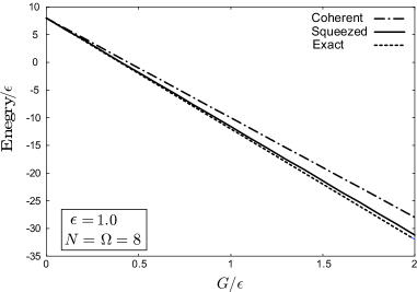
Fig. 1: Energy expectation values with respect to the coherent state (dot-dashed curve) and the squeezed state (solid curve) are depicted together with the exact eigenvalues (dotted curve) in the case $N=\mathchar 28938\relax=8$. The horizontal axis represents $G$ with the unit $\epsilon$.

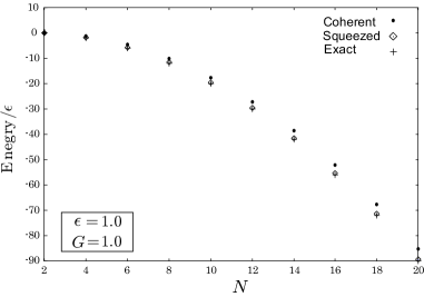
Fig. 2: Energy expectation values with respect to the coherent state (dots) and the squeezed state (diamonds) are depicted together with the exact eigenvalues (crosses) in the case $\epsilon=1.0$ and $G=1.0$. The horizontal axis represents $N$.

The result of the quasi-spin squeezed state well reproduces the exact eigenvalue for the wide range of $G$, comparing with the result by the coherent state.

In Fig.2, the energy is depicted in the case $\epsilon=1.0$ and $G=1$. The horizontal axis represents the particle number $N$ with $\mathchar 28938\relax=N$. The result obtained by using the quasi-spin squeezed state is almost same as the exact eigenvalue. These figures show that the squeezed state approach presents a good approximation.

5 Extension to O(4) model with pairing plus quadrapole interactions

In the previous sections, §§3 and 4, the $su(2)$-algebraic model with the pairing interaction has been investigated by using the quasi-spin squeezed state. It has been shown that the ground state energy has been well reproduced compared with the usual $su(2)$-coherent state. In this section, we try to extend our squeezed state approach to the $O(4)$-algebraic model with both the pairing and the quadrapole interactions in the many-fermion system such as nucleus.

5.1 O(4) model with pairing and quadrapole interactions

Let us start with the single-$j$ shell model, where $j$ represents the angular momentum quantum number. Thus, the degeneracy $2\mathchar 28938\relax$ is $2\mathchar 28938\relax=2j+1$. The pairing and the quadrapole interactions are active in this model. The Hamiltonian can be expressed as[13]

$${\hat{H}}_{\rm O(4)}=\epsilon{\hat{N}}-G{\hat{P}}^{\dagger}{\hat{P}}-\frac{\chi}{2}{\hat{Q}}^{2}\ .$$ (5.1)

Here, we define the following operators in terms of the fermion annihilation and creation operators $\{{\hat{c}}_{m},{\hat{c}}_{m}^{\dagger}\}$ as

$${\hat{P}}^{\dagger}=\sum_{m>0}^{j}{\hat{c}}_{m}^{\dagger}{\hat{c}}_{{\widetilde{m}}}^{\dagger}\ ,\qquad{\hat{P}}=\sum_{m>0}^{j}{\hat{c}}_{{\widetilde{m}}}{\hat{c}}_{m}\ ,$$

$${\hat{Q}}=\sum_{m=-j}^{j}\sigma_{m}{\hat{c}}_{m}^{\dagger}{\hat{c}}_{m}\ ,\qquad{\hat{N}}=\sum_{m=-j}^{j}{\hat{c}}_{m}^{\dagger}{\hat{c}}_{m}\ ,$$

$${{\widetilde{P}}}^{\dagger}=\sum_{m>0}^{j}\sigma_{m}{\hat{c}}_{m}^{\dagger}{\hat{c}}_{{\widetilde{m}}}^{\dagger}\ ,\qquad{{\widetilde{P}}}=\sum_{m>0}^{j}\sigma_{m}{\hat{c}}_{{\widetilde{m}}}{\hat{c}}_{m}\ ,$$ (5.2)

where

$${\hat{c}}_{{\widetilde{m}}}=(-)^{j-m}{c_{-m}}\ ,\qquad\sigma_{m}=\cases{1\ ,\quad{\rm for}\ |m|\leq\mathchar 28938\relax/2\cr-1\ ,\quad{\rm for}\ |m|>\mathchar 28938\relax/2}$$ (5.3)

and $\mathchar 28938\relax$ represents the half of the degeneracy. In (5.1), we also define ${\widetilde{P}}^{\dagger}$ and ${\widetilde{P}}$ for the later convenience.

The Hamiltonian (5.1) has the $O(4)$-algebraic structure. We can construct two $su(2)$-generators from the operators in (5.1) :

$${\hat{S}}_{+}^{\rm I}=({\hat{P}}^{\dagger}+{\widetilde{P}}^{\dagger})=\sum_{0<m\leq\mathchar 28938\relax/2}{\hat{c}}_{m}^{\dagger}{\hat{c}}_{\widetilde{m}}^{\dagger}=({\hat{S}}_{-}^{{\rm I}})^{\dagger}\ ,$$

$${\hat{S}}_{0}^{\rm I}=({\hat{N}}+{\hat{Q}}-\mathchar 28938\relax)/4=\left(2\sum_{|m|\leq\mathchar 28938\relax/2}{\hat{c}}_{m}^{\dagger}{\hat{c}}_{\widetilde{m}}-\mathchar 28938\relax\right)/4\ ,$$ (5.4a)

$${\hat{S}}_{+}^{{\rm O}}=({\hat{P}}^{\dagger}-{\widetilde{P}}^{\dagger})=\sum_{\mathchar 28938\relax/2<m\leq\mathchar 28938\relax}{\hat{c}}_{m}^{\dagger}{\hat{c}}_{\widetilde{m}}^{\dagger}=({\hat{S}}_{-}^{{\rm O}})^{\dagger}\ ,$$

$${\hat{S}}_{0}^{\rm O}=({\hat{N}}-{\hat{Q}}-\mathchar 28938\relax)/4=\left(2\sum_{\mathchar 28938\relax/2<|m|\leq\mathchar 28938\relax}{\hat{c}}_{m}^{\dagger}{\hat{c}}_{\widetilde{m}}-\mathchar 28938\relax\right)/4\ ,$$ (5.4b)

where these operators satisfy the following commutation relations :

$$[{\hat{S}}_{+}^{\rm I},{\hat{S}}_{-}^{\rm I}]=2{\hat{S}}_{0}^{\rm I}\ ,\qquad[{\hat{S}}_{0}^{\rm I},{\hat{S}}_{\pm}^{\rm I}]=\pm{\hat{S}}_{\pm}^{\rm I}\ ,$$

$$[{\hat{S}}_{+}^{\rm O},{\hat{S}}_{-}^{\rm O}]=2{\hat{S}}_{0}^{\rm O}\ ,\qquad[{\hat{S}}_{0}^{\rm O},{\hat{S}}_{\pm}^{\rm O}]=\pm{\hat{S}}_{\pm}^{\rm O}\ ,$$

$$[{\hat{S}}_{\pm,0}^{\rm I},{\hat{S}}_{\pm,0}^{\rm O}]=0\ .$$ (5.5)

Thus, the sets $\{{\hat{S}}_{\pm,0}^{\rm I}\}$ and $\{{\hat{S}}_{\pm,0}^{\rm O}\}$ give two sets of independent $su(2)$-generators. By expressing the operators ${\hat{P}}^{\dagger}$, ${\hat{P}}$ and ${\hat{N}}$ inversely in terms of the above two $su(2)$-generators, the Hamiltonian in (5.1) can be expressed in terms of two independent $su(2)$-generators. Thus, this model given by the Hamiltonian in (5.1) is called $O(4)\ (\simeq su(2)\times su(2))$ model. This model can be solved exactly because the model space is spanned by two quasi-spin $su(2)$ states and the diagonalization is easily performed. Thus, the validity of an approximation can be checked.

An approach by the $O(4)$-coherent state corresponds to the Hartree-Fock approximation. The $O(4)$-coherent state can be constructed by the direct product of the two $su(2)$-coherent state as

$$|{c}\rangle_{O(4)}=|{\alpha_{I}}\rangle\otimes|{\alpha_{O}}\rangle\equiv|{\alpha_{I},\alpha_{O}}\rangle\ ,$$

$$\quad|{\alpha_{I}}\rangle=\frac{1}{\sqrt{\mathchar 28936\relax_{I}}}\exp\left(\alpha_{I}\frac{{\hat{S}}_{+}^{\rm I}}{\sqrt{2S_{I}}}\right)|{0}\rangle_{I}\ ,\quad|{\alpha_{O}}\rangle=\frac{1}{\sqrt{\mathchar 28936\relax_{O}}}\exp\left(\alpha_{O}\frac{{\hat{S}}_{+}^{\rm O}}{\sqrt{2S_{O}}}\right)|{0}\rangle_{O}\ ,$$

$$\qquad\mathchar 28936\relax_{I}=\left(1+\frac{\alpha_{I}^{*}\alpha_{I}}{2S_{I}}\right)^{2S_{I}}\ ,\qquad\mathchar 28936\relax_{O}=\left(1+\frac{\alpha_{O}^{*}\alpha_{O}}{2S_{O}}\right)^{2S_{O}}\ ,$$

$$\qquad\quad S_{I}=\mathchar 28938\relax/4\ ,\qquad\qquad S_{O}=\mathchar 28938\relax/4\ .$$ (5.6)

Thus, the variational parameters are $\alpha_{I}$, $\alpha_{I}^{*}$, $\alpha_{O}$ and $\alpha_{O}^{*}$ in $O(4)$-coherent state.

For the number conservation, we introduce the chemical potential. Then, the variation with respect to $\alpha_{I}$, $\alpha_{I}^{*}$, $\alpha_{O}$ and $\alpha_{O}^{*}$ is carried out as

$$\delta\langle{\alpha_{I},\alpha_{O}}|{\hat{H}}_{O(4)}-\mu{\hat{N}}|{\alpha_{I},\alpha_{O}}\rangle=0\ .$$ (5.7)

Figure 3 shows the exact ground state energy eigenvalues (dotted curve) and the energy expectation value calculated by the $O(4)$-coherent state (dashed curve). The model parameters $G$ and $\chi$ are parameterized as $G=\cos\theta$ and $2\chi=\sin\theta$, respectively,[13] and $N=\mathchar 28938\relax=8$ and $\epsilon=0$. It is found that, if the quadrapole interaction is dominant, that is, $\theta$ is large, the coherent state approximation presents good results for the ground state energy. However, the pairing interaction is dominant, the coherent state approximation is rather bad. There is a room to devise the approximate state in the $O(4)$ model with the pairing and quadrapole interactions such as nucleus.

5.2 Direct product of two quasi-spin squeezed states

As is similar to the $su(2)$-squeezed state given in §3, let us construct the squeezed state for the $O(4)$ model. First, let us introduce the Bogoliubov transformed fermion annihilation and creation operators $({\hat{a}}_{m},{\hat{b}}_{m};{\hat{a}}_{m}^{\dagger},{\hat{b}}_{m}^{\dagger})$ :

$${\hat{a}}_{m}=U_{I}{\hat{c}}_{m}-V_{I}{\hat{c}}_{\widetilde{m}}^{\dagger}\ ,\quad{\rm for}\ \ |m|\leq\mathchar 28938\relax/2\ ,$$

$${\hat{b}}_{m}=U_{O}{\hat{c}}_{m}-V_{O}{\hat{c}}_{\widetilde{m}}^{\dagger}\ ,\quad{\rm for}\ \ \mathchar 28938\relax/2<|m|\leq\mathchar 28938\relax\ ,$$ (5.8)

where the coefficients of the Bogoliubov transformation are given as

$$U_{I}=\frac{1}{\sqrt{1+\alpha_{I}^{*}\alpha_{I}/(2S_{I})}}\ ,\quad V_{I}=\frac{\alpha_{I}}{\sqrt{2S_{I}}}\frac{1}{\sqrt{1+\alpha_{I}^{*}\alpha_{I}/(2S_{I})}}\ ,\quad U_{I}^{2}+|V|_{I}^{2}=1\ ,$$

$$U_{O}=\frac{1}{\sqrt{1+\alpha_{O}^{*}\alpha_{O}/(2S_{O})}}\ ,\quad V_{O}=\frac{\alpha_{O}}{\sqrt{2S_{O}}}\frac{1}{\sqrt{1+\alpha_{O}^{*}\alpha_{O}/(2S_{O})}}\ ,\quad U_{O}^{2}+|V|_{O}^{2}=1\ .$$

Then, the boson-like operators are introduced like (3.6) :

$${\hat{B}}_{I}^{\dagger}=\frac{1}{\sqrt{2S_{I}}}\sum_{0<m\leq\mathchar 28938\relax/2}{\hat{a}}_{m}^{\dagger}{\hat{a}}_{\widetilde{m}}^{\dagger}\ ,\>~{}\!{\hat{B}}_{I}=\frac{1}{\sqrt{2S_{I}}}\sum_{0<m\leq\mathchar 28938\relax/2}{\hat{a}}_{\widetilde{m}}{\hat{a}}_{m}\ ,\>~{}\!{\hat{M}}_{I}=\sum_{|m|\leq\mathchar 28938\relax/2}{\hat{a}}_{m}^{\dagger}{\hat{a}}_{m}\ ,$$

$${\hat{B}}_{O}^{\dagger}=\frac{1}{\sqrt{2S_{O}}}\sum_{\mathchar 28938\relax/2<m\leq\mathchar 28938\relax}{\hat{b}}_{m}^{\dagger}{\hat{b}}_{\widetilde{m}}^{\dagger}\ ,\>~{}\!{\hat{B}}_{O}=\frac{1}{\sqrt{2S_{O}}}\sum_{\mathchar 28938\relax/2<m\leq\mathchar 28938\relax}{\hat{b}}_{\widetilde{m}}{\hat{b}}_{m}\ ,\>~{}\!{\hat{M}}_{O}=\sum_{\mathchar 28938\relax/2<|m|}{\hat{b}}_{m}^{\dagger}{\hat{b}}_{m}\ .$$

Then, the following commutation relations are satisfied :

$$[{\hat{B}}_{I},{\hat{B}}_{I}^{\dagger}]=1-\frac{{\hat{M}}_{I}}{2S_{I}}\ ,\qquad[{\hat{M}}_{I},{\hat{B}}_{I}]=-2{\hat{B}}_{I}\ ,\qquad[{\hat{M}}_{I},{\hat{B}}_{I}^{\dagger}]=2{\hat{B}}_{I}^{\dagger}\ ,$$

$$[{\hat{B}}_{O},{\hat{B}}_{O}^{\dagger}]=1-\frac{{\hat{M}}_{O}}{2S_{O}}\ ,\quad[{\hat{M}}_{O},{\hat{B}}_{O}]=-2{\hat{B}}_{O}\ ,\quad[{\hat{M}}_{O},{\hat{B}}_{O}^{\dagger}]=2{\hat{B}}_{O}^{\dagger}\ .$$ (5.11)

The quasi-spin squeezed state $|{\psi}\rangle$ for $O(4)$ model may be constructed by the direct product of the two quasi-spin squeezed states, $|{\psi(\alpha_{I},\beta_{I})}\rangle$ and $|{\psi(\alpha_{O},\beta_{O})}\rangle$, which are defined as is similar to (3.1) :

$$|{\psi}\rangle=|{\psi(\alpha_{I},\beta_{I})}\rangle\otimes|{\psi(\alpha_{O},\beta_{O})}\rangle\ ,$$

$$\ \ |{\psi(\alpha_{I},\beta_{I})}\rangle=\frac{1}{\sqrt{\mathchar 28937\relax(\beta_{I}^{*}\beta_{I})}}\exp\left(\frac{1}{2}\beta_{I}{\hat{B}}_{I}^{\dagger 2}\right)|{\alpha_{I}}\rangle\ ,$$

$$\ \ |{\psi(\alpha_{O},\beta_{O})}\rangle=\frac{1}{\sqrt{\mathchar 28937\relax(\beta_{O}^{*}\beta_{O})}}\exp\left(\frac{1}{2}\beta_{O}{\hat{B}}_{O}^{\dagger 2}\right)|{\alpha_{O}}\rangle\ ,$$ (5.12)

$$\ \ \ \ \mathchar 28937\relax(\beta_{I}\beta_{I}^{*})=1+\sum_{k=1}^{[S_{I}]}\frac{(2k-1)!!}{(2k)!!}(|\beta_{I}|^{2})^{k}\prod_{p=1}^{2k-1}\left(1-\frac{p}{2S_{I}}\right)\ ,$$

$$\ \ \ \ \mathchar 28937\relax(\beta_{O}\beta_{O}^{*})=1+\sum_{k=1}^{[S_{O}]}\frac{(2k-1)!!}{(2k)!!}(|\beta_{O}|^{2})^{k}\prod_{p=1}^{2k-1}\left(1-\frac{p}{2S_{O}}\right)\ .$$

Since the two $su(2)$-generators are expressed in terms of the above introduced boson-like operators in (5.2) as

$${\hat{S}}_{+}^{\rm I}=2S_{I}\left(1-\frac{{\hat{M}}_{I}}{2S_{I}}\right)U_{I}V_{I}^{*}+\sqrt{2S_{I}}(U_{I}^{2}{\hat{B}}_{I}^{\dagger}-V_{I}^{*2}{\hat{B}}_{I})=({\hat{S}}_{-}^{\rm I})^{\dagger}\ ,$$

$${\hat{S}}_{0}^{\rm I}=-S_{I}(U_{I}^{2}-|V_{I}|^{2})\left(1-\frac{{\hat{M}}_{I}}{2S_{I}}\right)+\sqrt{2S_{I}}U_{I}(V_{I}{\hat{B}}_{I}+V_{I}^{*}{\hat{B}}_{I}^{\dagger})\ ,$$

$${\hat{S}}_{+}^{\rm O}=2S_{O}\left(1-\frac{{\hat{M}}_{O}}{2S_{O}}\right)U_{O}V_{O}^{*}+\sqrt{2S_{O}}(U_{O}^{2}{\hat{B}}_{O}^{\dagger}-V_{O}^{*2}{\hat{B}}_{O})=({\hat{S}}_{-}^{\rm O})^{\dagger}\ ,$$

$${\hat{S}}_{0}^{\rm O}=-S_{O}(U_{O}^{2}-|V_{O}|^{2})\left(1-\frac{{\hat{M}}_{O}}{2S_{O}}\right)+\sqrt{2S_{O}}U_{O}(V_{O}{\hat{B}}_{O}+V_{O}^{*}{\hat{B}}_{O}^{\dagger})\ .$$ (5.13)

Also, the pairing operator ${\hat{P}}$, the quadrapole operator ${\hat{Q}}$ and the number operator ${\hat{N}}$ can be expressed in terms of the above two sets of the $su(2)$-generators as

$${\hat{P}}={\hat{S}}_{-}^{\rm I}+{\hat{S}}_{-}^{\rm O}\ ,\quad{\hat{Q}}=2({\hat{S}}_{0}^{\rm I}-{\hat{S}}_{0}^{\rm O})\ ,\quad{\hat{N}}=2({\hat{S}}_{0}^{\rm I}+{\hat{S}}_{0}^{\rm O})+\mathchar 28938\relax\ .$$ (5.14)

Thus, the expectation value of the Hamiltonian (5.1) can be expressed by the $su(2)$-generators.

The variation are carried out with respect to the eight variational parameters $\alpha_{I,O}$, $\alpha_{I,O}^{*}$, $\beta_{I,O}$ and $\beta_{I,O}^{*}$ as

$$\delta\langle{\psi}|{\hat{H}}_{O(4)}-\mu{\hat{N}}|{\psi}\rangle=0\ .$$ (5.15)

The expectation values are summarized in Appendix A.

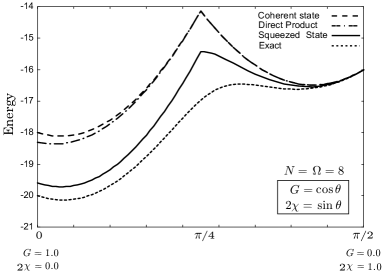
Fig. 3: Energy expectation values with respect to the coherent state (dashed curve), the direct product of two quasi-spin squeezed state (dot-dashed curve) and the fermionic squeezed state (solid curve) are depicted together with the exact eigenvalues (dotted curve) in the case $N=\mathchar 28938\relax=8$. The horizontal axis represents $\theta$ which parameterize the model parameters $G=\cos\theta$ and $2\chi=\sin\theta$.

The energy expectation value for this model Hamiltonian with respect to the direct product of the two quasi-spin squeezed state are depicted in Fig. 3 (dot-dashed curve) compared with the exact eigenvalues (dotted curve) and the expectation values derived by using the $O(4)$-coherent state (dashed curve) in the case $N=\mathchar 28938\relax=8$. The horizontal axis denotes $\theta$ where we parameterize the force strength $G$ and $\chi$ as $G=\cos\theta$ and $2\chi=\sin\theta$. It is found that the direct product of the two $su(2)$-spin squeezed states does not present good results for the ground state energy, especially in the region where the pairing interaction is dominant. The reason is as follows : If $\chi=0$, the $O(4)$ model is reduced to the pairing model investigated in §§2$\sim$ 4. However, the direct product of the two quasi-spin squeezed state is not reduced to the state in (3.1) because of the absence of the cross term ${\hat{B}}_{I}^{\dagger}{\hat{B}}_{O}^{\dagger}$, even if the parameters are set up as $\alpha_{I}=\alpha_{O}$ and $\beta_{I}=\beta_{O}$. Thus, in this case, the direct product does not include appropriate pairing correlations fully, and thus does not give a suitable squeezed state for many-fermion systems.

5.3 Fermionic squeezed state

In the previous subsection, the squeezed state for the $O(4)$ model has been constructed by the direct product of the two quasi-spin squeezed state. The extension of the $su(2)$-quasi-spin squeezed state to that for the $O(4)$ model may be natural from the viewpoint of the algebraic structure. However, the ground state energy is not reproduced so well. In this subsection, the trial state can be devised, which we call a fermionic squeezed state.

We define another squeezed state $|{s}\rangle$ as

$$|{s}\rangle=\frac{1}{\sqrt{\mathchar 28928\relax}}{\rm exp}\left[\beta_{I}\hat{B}_{I}^{\dagger}+\beta_{O}\hat{B}_{O}^{\dagger}\right]^{2}|{c}\rangle_{O(4)}\ ,$$ (5.16)

$$\ \mathchar 28928\relax=\sum_{n=0}^{[\mathchar 28938\relax/2]}\frac{[(2n)!]^{2}}{(n!)^{2}}\sum_{r=0}^{2n}\frac{|\beta_{I}|^{2r}|\beta_{O}|^{4n-2r}}{(2n-r)!r!}\prod_{p=1}^{r-1}\left(1-\frac{p}{2S_{I}}\right)\prod_{q=1}^{2n-r-1}\left(1-\frac{q}{2S_{O}}\right)\ .$$

The state $|{s}\rangle$ can be reduced to the quasi-spin squeezed state if the conditions $\alpha_{I}=\alpha_{O}$ and $\beta_{I}=\beta_{O}$ are imposed. Thus, the pairing correlations are fully taken into account. The necessary expectation values for calculating the expectation value of the Hamiltonian are summarized in Appendix B. Thus, we can derive the variational equations in Eq.(5.15). By solving the variational equations, we can obtain eight parameters $(\alpha_{I,O},\alpha_{I,O}^{*},\beta_{I,O},\beta_{I,O}^{*})$, and then the energy expectation value is evaluated. In Fig. 3, the energy expectation values calculated by using the state $|{s}\rangle$ are depicted (solid curve) compared with the energies of exact approach, coherent state approximation and the approximation by using the direct product of two quasi-spin squeezed state in (5.2). It is shown that our squeezed state approach with the state $|{s}\rangle$ presents good results.

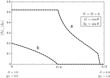
Fig. 4: The variables $|\beta_{I}|$ (solid curves) and $|\beta_{O}|$ (dashed curves) are depicted in the fermionic squeezed state approach (a) and the approach with the direct product of two quasi-spin squeezed state (b), respectively, in the case $N=\mathchar 28938\relax=8$. The horizontal axis represents $\theta$ which parameterize the model parameters $G=\cos\theta$ and $2\chi=\sin\theta$.

In Fig. 4, variables $|\beta_{I}|$ and $|\beta_{O}|$, which represent the quantum fluctuations and by which the particle-particle correlations are taken into account, are depicted in the case of the fermionic squeezed state (a) and the direct product of two quasi-spin squeezed state (b), respectively. In both cases, $|\beta_{I}|$ (solid curves) and $|\beta_{O}|$ (dashed curves) are almost the same. In all regions, the values $|\beta_{I}|$ and $|\beta_{O}|$ in the fermionic squeezed state approach are larger than those in the direct product of two quasi-spin squeezed state approach. Especially, in the fermionic squeezed state approach, it is found that the values are not negligible in the region where the pairing correlation is dominant. Thus, the pairing correlation is taken into account in this state. However, the values of $|\beta_{I}|$ and $|\beta_{O}|$ are rather small in the region where the quadrapole-quadrapole correlation is dominant. It may be concluded that the $O(4)$-coherent state is rather good state for describing the system in which the quadrapole correlation is rather strong.

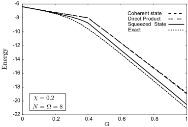
Fig. 5: Energy expectation values with respect to the coherent state (dashed curve), the direct product of two quasi-spin squeezed state (dot-dashed curve) and the fermionic squeezed state (solid curve) are depicted together with the exact eigenvalues (dotted curve) in the case $N=\mathchar 28938\relax=8$ and $\chi=0.2$. The horizontal axis represents $G$.

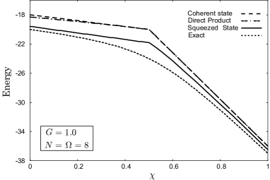
Fig. 6: Energy expectation values with respect to the coherent state (dashed curve), the direct product of two quasi-spin squeezed state (dot-dashed curve) and the fermionic squeezed state (solid curve) are depicted together with the exact eigenvalues (dotted curve) in the case $N=\mathchar 28938\relax=8$ and $G=1$. The horizontal axis represents $\chi$.

In Figs. 5 and 6, the energy expectation values with respect to the coherent state (dashed curve), the direct product of two quasi-spin squeezed state (dot-dashed curve) and the fermionic squeezed state (solid curve) are also depicted together with the exact eigenvalues (dotted curve) in the case $N=\mathchar 28938\relax=8$ with $\chi=0.2$ (Fig.5) and $G=1.0$ (Fig.6), respectively, in which the horizontal axes represent $G$ (Fig.5) and $\chi$ (Fig.6). It is found that the fermionic squeezed state approach presents rather good results in all the parameter regions with $G$ and $\chi$.

5.4 k-squeezed state

In this subsection, we give one comment. Let us consider the $su(2)$ pairing model discussed in §2 $\sim$ §4. We can define the $k$-squeezed state as

$$|{s}\rangle_{k}=\frac{1}{\sqrt{\mathchar 28928\relax_{k}}}\exp\left(\frac{w}{2}{\hat{B}}^{\dagger k}\right)|{\phi(\alpha)}\rangle\ ,\qquad(k\geq 3,\ ({\rm integer}))\ ,$$ (5.17)

$$\mathchar 28928\relax_{k}=\sum_{n=0}^{[\mathchar 28938\relax/k]}\frac{(kn)!}{4^{n}(n!)^{2}}|w|^{2n}\prod_{p=1}^{kn-1}\left(1-\frac{p}{2S_{j}}\right)\ .$$

In this state, the expectation values are calculated easily as

$${}_{k}\langle{s}|{\hat{B}}|{s}\rangle_{k}={}_{k}\langle{s}|{\hat{B}}^{\dagger}|{s}\rangle_{k}={}_{k}\langle{s}|{\hat{B}}^{2}|{s}\rangle_{k}={}_{k}\langle{s}|{\hat{B}}^{\dagger 2}|{s}\rangle_{k}=0\ ,$$

$${}_{k}\langle{s}|{\hat{M}}|{s}\rangle_{k}=\frac{1}{\mathchar 28928\relax_{k}}\sum_{n=0}^{[\mathchar 28938\relax/k]}(2kn)\frac{(kn)!}{(n!)^{2}}\frac{|w|^{2n}}{4^{n}}\prod_{p=1}^{kn-1}\left(1-\frac{p}{2S_{j}}\right)\ ,$$

$${}_{k}\langle{s}|{\hat{M}}^{2}|{s}\rangle_{k}=\frac{1}{\mathchar 28928\relax_{k}}\sum_{n=0}^{[\mathchar 28938\relax/k]}(2kn)^{2}\frac{(kn)!}{(n!)^{2}}\frac{|w|^{2n}}{4^{n}}\prod_{p=1}^{kn-1}\left(1-\frac{p}{2S_{j}}\right)\ ,$$

$${}_{k}\langle{s}|{\hat{B}}{\hat{B}}^{\dagger}|{s}\rangle_{k}=\frac{1}{\mathchar 28928\relax_{k}}\sum_{n=0}^{[\mathchar 28938\relax/k]}\frac{(kn+1)!}{(n!)^{2}}\frac{|w|^{2n}}{4^{n}}\prod_{p=1}^{kn}\left(1-\frac{p}{2S_{j}}\right)\ ,$$

$${}_{k}\langle{s}|{\hat{B}}^{\dagger}{\hat{B}}|{s}\rangle_{k}={}_{k}\langle{s}|{\hat{B}}{\hat{B}}^{\dagger}|{s}\rangle_{k}-\left(1-\frac{{}_{k}\langle{s}|{\hat{M}}|{s}\rangle_{k}}{2S_{j}}\right)\ ,$$ (5.18)

and the other combinations of the products of two operators give no finite values. In order to calculate the ground state energy, we impose the condition of minimization of the energy expectation value. As a result, it is concluded that $|w|=0$ is a solution for minimization. Thus, the $k$-squeezed state is reduced to the $su(2)$-coherent state in this pairing model. Therefore, the quasi-spin squeezed state gives a good state in order to take into account the pairing correlation.

6 summary

We have investigated a validity of the quasi-spin squeezed states as trial states in the variational method in the many-fermion systems with simple algebraic structures. First, we have applied the quasi-spin squeezed state to the pairing model by two approaches. One is dynamical approach, namely, the time-dependent variational approach. In this approach, the total fermion number is conserved automatically. We have imposed a consistency condition for the rotation in the phase space. As a result, the ground state energy is realized up to $O(1/\mathchar 28938\relax^{2},1/N^{2})$, which is better than the result of the coherent state approach, namely, the Hartree-Fock-Bogoliubov approximation. The other is to obtain the ground state energy directly in the energy minimum condition with the chemical potential. We have estimated the ground state energy numerically in the variational method, and compared the result with that of the coherent state approach and the exact energy eigenvalue. It has been shown that this quasi-spin squeezed state approach outrages the coherent state approach in all regions of the strength of the paring interaction.
Secondly, we have applied the quasi-spin squeezed state to the $O(4)$ model which has a $su(2)\times su(2)$ algebraic structure. Since we have the $su(2)$ quasi-spin squeezed state to take account the pairing correlation, we have adopted the direct product of two $su(2)$ quasi-spin squeezed states as a trial state. However, it has turned out that the quasi-spin squeezed state approach using the direct product of two quasi-spin squeezed states has not given good results compared with the $O(4)$-coherent state approach. The reason is that the pairing correlation can not be included appropriately, and the direct product of two quasi-spin squeezed states is not reduced to the quasi-spin squeezed state for pairing model when $\chi=0$. Thus, we have constructed another squeezed state free from the $O(4)$ algebra, which we call the fermionic squeezed state. This improved squeezed state includes partially the quadrapole correlation and is reduced to the quasi-spin squeezed state when two parameters are identical. Although the fermionic squeezed state has given rather good results than the direct product state, it may be not enough to include the quadrapole correlation when the quadrapole interaction is dominated ($G<2\chi$). This is the further problem to find more suitable state.
For further application of a quasi-spin squeezed state approach, it is interesting to investigate a nuclear $su(2)$-model which interact with the environment represented by a harmonic oscillator.[14] In this model, a certain case, a dissipative process has been realized. However, in our previous treatment,[14] a quantum fluctuation has not been took into account. Therefore, a quasi-spin squeezed state approach might be suitable to introduce and investigate the effect of quantum fluctuation into the system.

A Various expectation values by using the direct product of two quasi-spin squeezed states

In this appendix, we summarize the various expectation values with respect to the direct product of the quasi-spin squeezed states. We introduce new notations as $\mathchar 28937\relax(\beta_{I}\beta_{I}^{*})=\mathchar 28937\relax_{I}$, $\mathchar 28937\relax(\beta_{O}\beta_{O}^{*})=\mathchar 28937\relax_{O}$, $\mathchar 28937\relax^{\prime}_{I}=d\mathchar 28937\relax_{I}/d|\beta_{I}|^{2}$ and $\mathchar 28937\relax^{\prime}_{O}=d\mathchar 28937\relax_{O}/d|\beta_{O}|^{2}$.

$$\langle\psi|{\hat{M}}_{I}\hat{B}_{I}|\psi\rangle=\langle\psi|\hat{B}_{I}^{\dagger}{\hat{M}}_{I}|\psi\rangle=\langle\psi|\hat{B}_{I}{\hat{M}}_{I}|\psi\rangle=\langle\psi|{\hat{M}}_{I}\hat{B}_{I}^{\dagger}|\psi\rangle=0\ ,$$

$$\langle\psi|{\hat{M}}_{O}\hat{B}_{O}|\psi\rangle=\langle\psi|\hat{B}_{O}^{\dagger}{\hat{M}}_{O}|\psi\rangle=\langle\psi|\hat{B}_{O}{\hat{M}}_{O}|\psi\rangle=\langle\psi|{\hat{M}}_{O}\hat{B}_{O}^{\dagger}|\psi\rangle=0\ ,$$ (A.1)

$$\langle\psi|\hat{B}_{I}|\psi\rangle=\langle\psi|\hat{B}_{I}^{\dagger}|\psi\rangle=\langle\psi|\hat{B}_{O}|\psi\rangle=\langle\psi|\hat{B}_{O}^{\dagger}|\psi\rangle=0\ ,$$ (A.2)

$$\langle\psi|\hat{M}_{I}|\psi\rangle=4|\beta_{I}|^{2}\frac{\mathchar 28937\relax^{\prime}_{I}}{\mathchar 28937\relax_{I}},~{}~{}~{}~{}\langle\psi|\hat{M}_{O}|\psi\rangle=4|\beta_{O}|^{2}\frac{\mathchar 28937\relax_{O}^{\prime}}{\mathchar 28937\relax_{O}}\ ,$$ (A.3)

$$\langle\psi|\hat{M}_{I}^{2}|\psi\rangle=16|\beta_{I}|^{2}\frac{\mathchar 28937\relax^{\prime}_{I}}{\mathchar 28937\relax_{I}}+16|\beta_{I}|^{4}\frac{\mathchar 28937\relax^{\prime\prime}_{I}}{\mathchar 28937\relax_{I}}\ ,~{}~{}~{}~{}$$

$$\langle\psi|\hat{M}_{O}^{2}|\psi\rangle=16|\beta_{O}|^{2}\frac{\mathchar 28937\relax_{O}}{\mathchar 28937\relax_{O}}+16|\beta_{O}|^{4}\frac{{\mathchar 28937\relax_{O}}\!^{\prime\prime}}{\mathchar 28937\relax_{O}}\ .$$ (A.4)

$$\langle\psi|\hat{B}_{I}^{\dagger}\hat{B}_{I}|\psi\rangle=2|\beta_{I}|^{2}\left(1-\frac{1}{2S_{I}}\right)\frac{\mathchar 28937\relax^{\prime}_{I}}{\mathchar 28937\relax_{I}}-\frac{4|\beta_{I}|^{4}}{2S_{I}}\frac{\mathchar 28937\relax^{\prime\prime}_{I}}{\mathchar 28937\relax_{I}},~{}~{}~{}~{}$$

$$\langle\psi|\hat{B}_{O}^{\dagger}\hat{B}_{O}|\psi\rangle=2|\beta_{O}|^{2}\left(1-\frac{1}{2S_{O}}\right)\frac{\mathchar 28937\relax^{\prime}_{O}}{\mathchar 28937\relax_{O}}-\frac{4|\beta_{O}|^{4}}{2S_{O}}\frac{\mathchar 28937\relax^{\prime\prime}_{O}}{\mathchar 28937\relax_{O}}\ ,$$ (A.5)

$$\langle\psi|{\hat{B}}_{I}{\hat{B}}_{I}^{\dagger}|\psi\rangle=\langle\psi|{\hat{B}}_{I}^{\dagger}{\hat{B}}_{I}|\psi\rangle+\left(1-\frac{\langle\psi|{\hat{M}}_{I}|\psi\rangle}{2S_{I}}\right),~{}~{}~{}~{}$$

$$\langle\psi|{\hat{B}}_{O}{\hat{B}}_{O}^{\dagger}|\psi\rangle=\langle\psi|{\hat{B}}_{O}^{\dagger}{\hat{B}}_{O}|\psi\rangle+\left(1-\frac{\langle\psi|M_{O}|\psi\rangle}{2S_{O}}\right)\ ,$$ (A.6)

$$\langle{\psi}|{\hat{B}}_{I}^{2}|{\psi}\rangle=2\beta_{I}\frac{\mathchar 28937\relax_{I}^{\prime}}{\mathchar 28937\relax_{I}}\ ,\qquad\langle{\psi}|{\hat{B}}_{I}^{\dagger 2}|{\psi}\rangle=2\beta_{I}^{*}\frac{\mathchar 28937\relax_{I}^{\prime}}{\mathchar 28937\relax_{I}}\ ,$$

$$\langle{\psi}|{\hat{B}}_{O}^{2}|{\psi}\rangle=2\beta_{O}\frac{\mathchar 28937\relax_{O}^{\prime}}{\mathchar 28937\relax_{O}}\ ,\qquad\langle{\psi}|{\hat{B}}_{O}^{\dagger 2}|{\psi}\rangle=2\beta_{O}^{*}\frac{\mathchar 28937\relax_{O}^{\prime}}{\mathchar 28937\relax_{O}}\ .$$ (A.7)

Thus, the expectation value of the Hamiltonian in (5.1) can be calculated by using the above expectation values.

B Various expectation values by using the fermionic squeezed state

In this appendix, we summarize the various expectation values with respect to the fermionic squeezed state developed in §5-3.

$$\langle s|{\hat{M}}_{I}|s\rangle=\frac{1}{\mathchar 28928\relax}\Biggl{\{}~{}\!\sum_{n=0}^{[\frac{\mathchar 28938\relax}{2}]}\frac{[(2n)!]^{2}}{(n!)^{2}}~{}\!\sum_{r=0}^{2n}|\beta_{I}|^{2r}~{}\!|\beta_{O}|^{4n-2r}\frac{2r}{r!~{}\!(2n-r)!}$$

$$\qquad\qquad\qquad\qquad\times\prod^{r-1}_{p=1}\left(1-\frac{p}{2S_{I}}\right)\prod^{(2n-r-1)}_{q=1}\left(1-\frac{q}{2S_{O}}\right)\Biggr{\}}\ ,$$

$$\langle s|{\hat{M}}_{O}|s\rangle=\frac{1}{\mathchar 28928\relax}\Biggl{\{}~{}\!\sum_{n=0}^{[\frac{\mathchar 28938\relax}{2}]}\frac{[(2n)!]^{2}}{(n!)^{2}}~{}\!\sum_{r=0}^{2n}|\beta_{O}|^{2r}~{}\!|\beta_{I}|^{4n-2r}\frac{2r}{r!~{}\!(2n-r)!}$$

$$\qquad\qquad\qquad\qquad\times\prod^{r-1}_{p=1}\left(1-\frac{p}{2S_{O}}\right)\prod^{(2n-r-1)}_{q=1}\left(1-\frac{q}{2S_{I}}\right)\Biggr{\}}\ ,$$

(B.1)

$$\langle s|{\hat{M}}_{I}^{2}|s\rangle=\frac{1}{\mathchar 28928\relax}\Biggl{\{}~{}\!\sum_{n=0}^{[\frac{\mathchar 28938\relax}{2}]}\frac{[(2n)!]^{2}}{(n!)^{2}}~{}\!\sum_{r=0}^{2n}|\beta_{I}|^{2r}~{}\!|\beta_{O}|^{4n-2r}\left(1-\frac{p}{2S_{I}}\right)$$

$$\qquad\qquad\qquad\times\prod^{(2n-r-1)}_{q=1}\left(1-\frac{q}{2S_{O}}\right)\Biggr{\}}\ ,$$

$$\langle s|{\hat{M}}_{O}^{2}|s\rangle=\frac{1}{\mathchar 28928\relax}\Biggl{\{}~{}\!\sum_{n=0}^{[\frac{\mathchar 28938\relax}{2}]}\frac{[(2n)!]^{2}}{(n!)^{2}}~{}\!\sum_{r=0}^{2n}|\beta_{O}|^{2r}~{}\!|\beta_{I}|^{4n-2r}\frac{4r^{2}}{r!~{}\!(2n-r)!}$$

$$\qquad\qquad\qquad\qquad\times\prod^{r-1}_{p=1}\left(1-\frac{p}{2S_{O}}\right)\prod^{(2n-r-1)}_{q=1}\left(1-\frac{q}{2S_{I}}\right)\Biggr{\}}\ ,$$

$$\langle s|{\hat{M}}_{I}{\hat{M}}_{O}|s\rangle=\langle s|{\hat{M}}_{O}{\hat{M}}_{I}|s\rangle$$

$$\ \ =\frac{1}{\mathchar 28928\relax}\Biggl{\{}~{}\!\sum_{n=0}^{[\frac{\mathchar 28938\relax}{2}]}\frac{[(2n)!]^{2}}{(n!)^{2}}\sum_{r=0}^{2n}|\beta_{I}|^{2r}~{}\!|\beta_{O}|^{4n-2r}\frac{4r~{}\!(2n-r)}{r!~{}\!(2n-r)!}~{}\!$$

$$\qquad\qquad\qquad\qquad\times\prod^{r-1}_{p=1}\left(1-\frac{p}{2S_{I}}\right)\prod^{2n-r-1}_{q=1}\left(1-\frac{q}{2S_{O}}\right)\Biggr{\}}\ ,$$

(B.2)

$$\langle s|{\hat{B}}_{I}{\hat{B}}_{I}^{\dagger}|s\rangle=\frac{1}{\mathchar 28928\relax}\Biggl{\{}~{}\!\sum^{[\frac{\mathchar 28938\relax}{2}]}_{n=0}\frac{[(2n)!]^{2}}{(n!)^{2}}\sum_{r=0}^{2n}|\beta_{I}|^{2r}~{}\!|\beta_{O}|^{4n-2r}\frac{(r+1)}{r!~{}\!(2n-r)!}$$

$$\qquad\qquad\qquad\qquad\times\prod^{r}_{p=1}\left(1-\frac{p}{2S_{I}}\right)\prod^{2n-r-1}_{q=1}\left(1-\frac{q}{2S_{O}}\right)\Biggr{\}}\ ,$$

$$\langle s|{\hat{B}}_{O}{\hat{B}}_{O}^{\dagger}|s\rangle=\frac{1}{\mathchar 28928\relax}\Biggl{\{}~{}\!\sum^{[\frac{\mathchar 28938\relax}{2}]}_{n=0}\frac{[(2n)!]^{2}}{(n!)^{2}}\sum_{r=0}^{2n}|\beta_{O}|^{2r}~{}\!|\beta_{I}|^{4n-2r}\frac{(r+1)}{r!~{}\!(2n-r)!}$$

$$\qquad\qquad\qquad\qquad\times\prod^{r}_{p=1}\left(1-\frac{p}{2S_{O}}\right)\prod^{2n-r-1}_{q=1}\left(1-\frac{q}{2S_{I}}\right)\Biggr{\}}\ ,$$

(B.3)

$$\langle s|{\hat{B}}_{I}^{\dagger 2}|s\rangle=\frac{1}{\mathchar 28928\relax}\Biggl{\{}~{}\!\sum_{n=0}^{[\frac{\mathchar 28938\relax}{2}]}\frac{(2n)!~{}\!(2n+2)!}{n!\!~{}(n+1)!}\sum_{r=0}^{2n}\frac{\beta_{I}^{2}|\beta_{I}|^{2r}~{}\!|\beta_{O}|^{4n-2r}}{r!~{}\!(2n-r)!}$$

$$\qquad\qquad\qquad\qquad\times\prod^{r+1}_{p=1}\left(1-\frac{p}{2S_{I}}\right)\prod^{(2n-r-1)}_{q=1}\left(1-\frac{q}{2S_{O}}\right)\Biggr{\}}\ ,$$

$$\langle s|B_{O}^{\dagger 2}|s\rangle=\frac{1}{\mathchar 28928\relax}\Biggl{\{}~{}\!\sum_{n=0}^{[\frac{\mathchar 28938\relax}{2}]}\frac{(2n)!~{}\!(2n+2)!}{n!\!~{}(n+1)!}\sum_{r=0}^{2n}\frac{\beta_{O}^{2}|\beta_{O}|^{2r}~{}\!|\beta_{I}|^{4n-2r}}{r!~{}\!(2n-r)!}$$

$$\qquad\qquad\qquad\qquad\times\prod^{r+1}_{p=1}\left(1-\frac{p}{2S_{O}}\right)\prod^{(2n-r-1)}_{q=1}\left(1-\frac{q}{2S_{I}}\right)\Biggr{\}}\ ,$$

(B.4)

$$\langle s|{\hat{B}}_{I}{\hat{B}}_{O}|s\rangle=\frac{1}{\mathchar 28928\relax}\Biggl{\{}~{}\!\sum^{[\frac{\mathchar 28938\relax}{4}]}_{n=0}\frac{(2n)!(2n+2)!}{n!~{}\!(n+1)!}\sum^{2n}_{r=0}\frac{\beta_{I}\beta_{O}|\beta_{I}|^{2r}~{}\!|\beta_{O}|^{4n-2r}}{r!~{}\!(2n-r)!}$$

$$\qquad\qquad\qquad\qquad\times\prod^{r}_{p=1}\left(1-\frac{p}{2S_{I}}\right)\prod^{2n-r}_{q=1}\left(1-\frac{q}{2S_{O}}\right)\Biggr{\}}\ ,$$

$$\langle s|{\hat{B}}_{I}^{\dagger}{\hat{B}}_{O}|s\rangle=\frac{1}{\mathchar 28928\relax}\Biggl{\{}~{}\!\sum^{[\frac{\mathchar 28938\relax}{2}]}_{n=0}\frac{[(2n)!]^{2}}{(n!)^{2}}\sum_{r=0}^{2n}\beta_{I}^{*}\beta_{O}|\beta_{I}|^{2r}~{}\!|\beta_{O}|^{4n-2r-2}~{}\!\frac{(2n-r)}{r!~{}\!(2n-r)!}$$

$$\qquad\qquad\qquad\qquad\times\prod^{r}_{p=1}\left(1-\frac{p}{2S_{I}}\right)\prod^{2n-r-1}_{q=1}\left(1-\frac{q}{2S_{O}}\right)~{}\!\Biggl{\}}\ .$$ (B.5)

The expectation values of other products of two operators, except for the complex conjugates of the above operators, are zero.

References

- [1] Y. Tsue, A. Kuriyama and M. Yamamura, Prog. Theor. Phys. 92 (1994), 545.
- [2] Y. Tsue, N. Azuma, A. Kuriyama and M. Yamamura, Prog. Theor. Phys. 96 (1996), 729.
- [3] H. J. Lipkin, N. Meshkov and A. J. Glick, Nucl. Phys. 62 (1965), 188.
- [4] Y. Tsue, N. Azuma, A. Kuriyama and M. Yamamura, NASA Conference Publication, NASA/CP-1998-206855 (1998), 221.
- [5] A. Kuriyama, J. da Providência, Y. Tsue and M. Yamamura, Prog. Theor. Phys. Suppl. 141 (2001), 113.
- [6] Y. Tsue and H. Akaike, submitted to Prog. Theor. Phys.
- [7] T. Nakatsukasa and N. Walet, Phys. Rev. C58 (1998), 3397.
- [8] M. Kobayasi, T. Nakatsukasa, M. Matsuo and K. Matsuyanagi, Prog. Theor. Phys. 110 (2003), 65.
- [9] A. K. Kerman, Ann. of Phys. 12 (1961), 300.
- [10] R. D. Lawson and M. H. Macfarlane, Nucl. Phys. 66 (1965), 80.
- [11] See, for example, J. M. Eisenberg and W. Greiner, Nuclear Theory Vol.3.
- [12] M. Yamamura, private communication (unpublished work).
- [13] K. Matsuyanagi, Prog. Theor. Phys. 67 (1982), 1441.
- [14] H. Akaike, Y. Tsue, C. Providência, J. da Providência ,A. Kuriyama and M. Yamamura Prog. Theor. Phys. 105 (2001), 717.