A Possible Extension of a Trial State in the TDHF Theory with Canonical Form in the Lipkin Model

1 Introduction

The time-dependent Hartree-Fock (TDHF) theory is one of powerful methods to investigate the dynamics of quantum many-fermion systems. Especially, this theory has been developed in nuclear many-body problems.[1] The TDHF theory and the Hartree-Fock approximation are formulated based on the variational method. In these methods, the trial state for the variation is prepared to describe the many-fermion system. The Slater determinant is usually adopted as a possible trial state. This state gives a possible classical counterpart of the quantum many-fermion system. For this purpose, the TDHF theory with the canonical form presents a suitable treatment. In this treatment, the canonicity condition plays an essential and a central role.[2, 3] This trial state however may be regarded as a kind of the coherent state.

On the other hand, in the many-boson systems, the coherent state also gives the classical image of quantum many-boson systems. We have been formulated the time-dependent variational approach to quantum many-boson systems including appropriate quantum fluctuations for the systems under consideration.[4, 5] Then, the squeezed state is applied to the variation as a possible trial state.

In quantum many-fermion systems, one of the present authors (Y.T.) together with Yamamura and Kuriyama have constructed the trial state in both the pairing[6] and the Lipkin models[7] corresponding to the boson squeezed state. In these models, the Hamiltonian can be expressed in terms of the quasi-spin operators. Then, the Slater determinantal state is identical with the $su(2)$-coherent state. In this sense, we thus call the extended trial state the quasi-spin squeezed state. We have constructed the variational approximation, which include the result of the Hartree-Fock approximation, in the Lipkin model.[7] Then, this variational method using the quasi-spin squeezed state gives the results obtained in the random phase approximation (RPA) in the certain approximation.[8, 5] As a result, our quasi-spin squeezed state approach to the Lipkin model is a possible extension of the Hartree-Fock approximation.

In this paper, with the aim of extension of our previous work to the time-dependent variational approach to the Lipkin model, we investigate a possible solution of the canonicity condition in the quasi-spin squeezed state. The canonicity condition plays a central role to formulate the TDHF theory in the canonical form. Thus, we can construct the extended TDHF theory in the canonical form, if we use the quasi-spin squeezed state as a trial state instead of the Slater determinant. Also, the effect of the zero-point oscillation induced by the uncertainty principle is investigated in terms of the canonical variables. In this paper, the ground state energy is calculated by imposing a condition of minimum uncertainty relation in order to consider the above-mentioned zero-point oscillation. The comparison of the ground state energies obtained by various states, except for the quasi-spin squeezed state investigated in this paper, is also reported in ?.

This paper is organized as follows. In the next section, the Lipkin model is recapitulated containing the notations. In §3, the Slater determinant is used to describe the Lipkin model. In §4, a possible extension of the trial state for the variation is given. This state corresponds to the boson coherent state in the many-boson systems. Further, the canonicity conditions are imposed and a possible solutions of these conditions are given. Also, the way to obtain the approximate solution is discussed. The original idea to solve the canonicity condition is found in Ref.?. In §5, the energy expectation value is calculated including the zero-point fluctuation induced by the uncertainty principle. The last section is devoted to a summary.

2 Recapitulation of the Lipkin model

In this paper, we give a possible extension of the TDHF theory in the case of the Lipkin model. We consider $2\mathchar 28938\relax$ fermions moving in two single-particle levels with the same degeneracy $2\mathchar 28938\relax$. Here, $\mathchar 28938\relax$ is a positive integer, and for the convenience of later treatment, we use a half-integer $j$ defined by $\mathchar 28938\relax=j+1/2$ and an additional quantum number $m$ to distinguish each single-particle state. As the free vacuum $|{0}\rangle$, we can adopt a state in which one level is occupied by all fermions under consideration. This level may be called hole-level and the other particle-level. In this model, we introduce the following set of operators :

$${\hat{S}}_{+}=\sum_{m}a_{jm}^{*}(-)^{j-m}b_{j-m}^{*}\ ,$$

$${\hat{S}}_{-}=\sum_{m}(-)^{j-m}b_{j-m}a_{jm}\ ,$$

$${\hat{S}}_{0}=1/2\cdot\sum_{m}(a_{jm}^{*}a_{jm}+b_{jm}^{*}b_{jm})-\mathchar 28938\relax\ .$$ (2.1)

Here, $m$ runs from $-j$ to $+j$ and $(a_{jm}^{*},a_{jm})$ and $(b_{jm}^{*},b_{jm})$ denote particle and hole operators in the particle and hole state $jm$, respectively. They are fermion operators. The set $({\hat{S}}_{+},{\hat{S}}_{-},{\hat{S}}_{0})$ satisfies the $su(2)$ algebra obeying the relations

$$[\ {\hat{S}}_{-}\ ,\ {\hat{S}}_{+}\ ]=-2{\hat{S}}_{0}\ ,\qquad[\ {\hat{S}}_{0}\ ,\ {\hat{S}}_{\pm}\ ]=\pm{\hat{S}}_{\pm}\ .$$ (2.2)

In order to give a transparent connection to boson system, which we have already given the form, it may be convenient to define the quantities

$${\hat{A}}^{*}={\hat{S}}_{+}/\sqrt{2\mathchar 28938\relax}\ ,\quad{\hat{A}}={\hat{S}}_{-}/\sqrt{2\mathchar 28938\relax}\ ,\quad{\hat{N}}=2(\mathchar 28938\relax+{\hat{S}}_{0})\ .$$ (2.3)

The set $({\hat{A}}^{*},{\hat{A}},{\hat{N}})$ satisfies the relations

$$[\ {\hat{A}}\ ,\ {\hat{A}}^{*}\ ]=1-{\hat{N}}/2\mathchar 28938\relax\ ,\quad[\ {\hat{N}}\ ,\ {\hat{A}}^{*}\ ]=+2{\hat{A}}^{*}\ ,\quad[\ {\hat{N}}\ ,\ {\hat{A}}\ ]=-2{\hat{A}}\ .$$ (2.4)

The first relation shows that if ${\hat{N}}/2\mathchar 28938\relax$ is negligible, the operators ${\hat{A}}$ and ${\hat{A}}^{*}$ can be regarded as boson operators. Further, we define ${\hat{Q}}$, ${\hat{P}}$ and ${\hat{R}}$ in the following forms :

$${\hat{Q}} = \sqrt{\hbar/2}\cdot({\hat{A}}^{*}+{\hat{A}})$$

$$= \sqrt{\hbar/2}\cdot({\hat{S}}_{+}+{\hat{S}}_{-})/\sqrt{2\mathchar 28938\relax}=\sqrt{\hbar/\mathchar 28938\relax}\cdot{\hat{S}}_{x}\ ,$$

$${\hat{P}} = i\sqrt{\hbar/2}\cdot({\hat{A}}^{*}-{\hat{A}})$$

$$= i\sqrt{\hbar/2}\cdot({\hat{S}}_{+}-{\hat{S}}_{-})/\sqrt{2\mathchar 28938\relax}=-\sqrt{\hbar/\mathchar 28938\relax}\cdot{\hat{S}}_{y}\ ,$$

$${\hat{R}} = 1-{\hat{N}}/2\mathchar 28938\relax=-{\hat{S}}_{0}/\mathchar 28938\relax=-{\hat{S}}_{z}/\mathchar 28938\relax\ .$$ (2.5)

The operators ${\hat{Q}}$, ${\hat{P}}$ and ${\hat{R}}$ satisfy the relations

$${\hat{Q}}^{*}={\hat{Q}}\ ,\qquad{\hat{P}}^{*}={\hat{P}}\ ,\qquad{\hat{R}}^{*}={\hat{R}}\ ,$$ (2.6)

$$[\ {\hat{Q}}\ ,\ {\hat{P}}\ ]=i\hbar{\hat{R}}\ .$$ (2.7)

In this case, also, if ${\hat{N}}/2\mathchar 28938\relax$ is negligible, ${\hat{Q}}$ and ${\hat{P}}$ can be regarded as the coordinate and its canonical momentum and ${\hat{R}}$ becomes unit operator.

For the operators ${\hat{Q}}$ and ${\hat{P}}$ satisfying the relations (2.6) and (2.7), we have the following uncertainty relation :

$$\mathchar 28929\relax Q\cdot\mathchar 28929\relax P\geq\hbar/2\cdot|\langle{\hat{R}}\rangle|\ .$$ (2.8)

Here, $\mathchar 28929\relax Q$ and $\mathchar 28929\relax P$ are defined by

$$\mathchar 28929\relax Q=\sqrt{\langle({\hat{Q}}-\langle{\hat{Q}}\rangle)^{2}\rangle}\ ,\qquad\mathchar 28929\relax P=\sqrt{\langle({\hat{P}}-\langle{\hat{P}}\rangle)^{2}\rangle}\ .$$ (2.9)

The symbol $\langle{\hat{O}}\rangle$ denotes the expectation value of the operator ${\hat{O}}$ for an arbitrary state $|{\ }\rangle$. This relation can be proved by preparing the relations

$$\langle{\hat{Y}}^{*}{\hat{Y}}\rangle\geq 0\ ,\quad({\rm positive\ definite})$$ (2.10)

where, for arbitrary real number $y$, ${\hat{Y}}^{*}$ and ${\hat{Y}}$ are defined as

$${\hat{Y}}^{*}=({\hat{P}}-\langle{\hat{P}}\rangle)y+i({\hat{Q}}-\langle{\hat{Q}}\rangle)\ ,$$

$${\hat{Y}}=({\hat{P}}-\langle{\hat{P}}\rangle)y-i({\hat{Q}}-\langle{\hat{Q}}\rangle)\ .$$ (2.11)

3 Slater determinant as a trial state for the variation

First, we introduce the following state :

$$|{\phi(A)}\rangle=1/\sqrt{\mathchar 28936\relax(A^{*}A)}\cdot\exp(A{\hat{A}}^{*})|{0}\rangle\ ,$$ (3.1)

where $\mathchar 28936\relax(A^{*}A)$ is given by

$$\mathchar 28936\relax(A^{*}A)=\langle{0}|\exp(A^{*}{\hat{A}})\cdot\exp(A{\hat{A}}^{*})|{0}\rangle=(1+A^{*}A/2\mathchar 28938\relax)^{2\mathchar 28938\relax}\ .$$ (3.2)

The state $|{\phi(A)}\rangle$ is a Slater determinant with the condition

$$\langle{\phi(A)}|\phi(A)\rangle=1\ .$$ (3.3)

The factor $\sqrt{\mathchar 28936\relax(A^{*}A)}$ reduces to $\exp(A^{*}A/2)$ at the limit $A^{*}A/2\mathchar 28938\relax\rightarrow 0$ and the state $|{\phi(A)}\rangle$ becomes a coherent state in boson system.

With the help of the following canonicity condition, we introduce a set of canonical variables $(X^{*},X)$ :

$$\langle{\phi(A)}|\partial_{X}|{\phi(A)}\rangle=X^{*}/2\ .$$ (3.4)

Of course, the variables $X^{*}$ and $X$ obey the Poisson bracket relation $\{X,X^{*}\}_{P}=1$. Further, the equation of motion for $X^{*}$ and $X$ are given by the variational principle. The explicit calculation of the left-hand side of Eq.(3.4) gives

$$\langle{\phi(A)}|\partial_{X}|{\phi(A)}\rangle=1/(1+A^{*}A/2\mathchar 28938\relax)\cdot(A^{*}\partial_{X}A-A\partial_{X}A^{*})/2\ .$$ (3.5)

A possible solution of Eqs.(3.4) and (3.5) is given by

$$A^{*}=X^{*}/\sqrt{1-X^{*}X/2\mathchar 28938\relax}\ ,\qquad A=X/\sqrt{1-X^{*}X/2\mathchar 28938\relax}\ .$$ (3.6)

With the use of the above relations (3.6), we can express all relations in our present treatment in terms of $X^{*}$ and $X$.

The TDHF theory in the Lipkin model consists of the expectation values of the operators ${\hat{A}}^{*}$, ${\hat{A}}$ and ${\hat{N}}$ for the state $|{\phi(A)}\rangle$ :

$$\langle{\phi}|{\hat{A}}^{*}|{\phi}\rangle=X^{*}\sqrt{1-X^{*}X/2\mathchar 28938\relax}\ ,$$

$$\langle{\phi}|{\hat{A}}|{\phi}\rangle=X\sqrt{1-X^{*}X/2\mathchar 28938\relax}\ ,$$ (3.7)

$$\langle{\phi}|{\hat{N}}|{\phi}\rangle=2X^{*}X\ ,\qquad\langle{\phi}|1-{\hat{N}}/2\mathchar 28938\relax|{\phi}\rangle=1-X^{*}X/\mathchar 28938\relax\ .$$ (3.8)

The above expectation values are for the state $|{\phi(A)}\rangle$. We can see that they are classical counterparts of the Holstein-Primakoff type boson representation of the $su(2)$ algebra. If $X^{*}X/2\mathchar 28938\relax$ is negligible, the relations (3.7) show that the expectation values of ${\hat{A}}^{*}$ and ${\hat{A}}$ are reduced to the canonical variables $X^{*}$ and $X$. Then, the factor $\sqrt{1-X^{*}X/2\mathchar 28938\relax}$ can be attributed to the blocking effect, a kind of quantum effects, which comes from the exclusion principle. As was mentioned in §1, our main interest is to clarify the effect of the zero-point oscillation induced by the uncertainty principle. Therefore, as our terminology, we include the blocking effect in the classical counterpart.

With the aim of investigating the effect of the uncertainty principle, we calculate the square order of the expectation values of the operators ${\hat{A}}^{*}$, ${\hat{A}}$ and ${\hat{N}}$ :

$$\langle{\phi}|{\hat{A}}^{*2}|{\phi}\rangle=X^{*2}(1-X^{*}X/2\mathchar 28938\relax)(1-1/2\mathchar 28938\relax)\ ,$$

$$\langle{\phi}|{\hat{A}}^{2}|{\phi}\rangle=X^{2}(1-X^{*}X/2\mathchar 28938\relax)(1-1/2\mathchar 28938\relax)\ ,$$ (3.9)

$$\langle{\phi}|{\hat{A}}^{*}{\hat{A}}|{\phi}\rangle=X^{*}X(1-X^{*}X/2\mathchar 28938\relax)+(X^{*}X/2\mathchar 28938\relax)^{2}\ ,$$

$$\langle{\phi}|{\hat{A}}{\hat{A}}^{*}|{\phi}\rangle=X^{*}X(1-X^{*}X/2\mathchar 28938\relax)+(1-X^{*}X/2\mathchar 28938\relax)^{2}$$

$$\qquad\qquad\ \ =\langle{\phi}|{\hat{A}}^{*}{\hat{A}}|{\phi}\rangle+(1-X^{*}X/\mathchar 28938\relax)\ ,$$ (3.10)

$$\langle{\phi}|(1-{\hat{N}}/2\mathchar 28938\relax)^{2}|{\phi}\rangle=(1-X^{*}X/\mathchar 28938\relax)^{2}+1/\mathchar 28938\relax\cdot X^{*}X/\mathchar 28938\relax\cdot(1-X^{*}X/2\mathchar 28938\relax)\ .\qquad$$ (3.11)

Using the above relations, we can set the following result for the state $|{\phi(A)}\rangle$ :

$$(\mathchar 28929\relax Q)^{2}=\langle{\phi}|{\hat{Q}}^{2}|{\phi}\rangle-\langle{\phi}|{\hat{Q}}|{\phi}\rangle^{2}$$

$$\qquad\quad=\hbar/2\cdot[1-(X^{*}X+X^{*2})/2\mathchar 28938\relax][1-(X^{*}X+X^{2})/2\mathchar 28938\relax]\ ,$$ (3.12)

$$(\mathchar 28929\relax P)^{2}=\langle{\phi}|{\hat{P}}^{2}|{\phi}\rangle-\langle{\phi}|{\hat{P}}|{\phi}\rangle^{2}$$

$$\qquad\quad=\hbar/2\cdot[1-(X^{*}X-X^{*2})/2\mathchar 28938\relax][1-(X^{*}X-X^{2})/2\mathchar 28938\relax]\ ,$$ (3.13)

$$\langle{\phi}|{\hat{Q}}|{\phi}\rangle=\sqrt{\hbar/2}\cdot(X^{*}+X)\sqrt{1-X^{*}X/2\mathchar 28938\relax}\ ,$$ (3.14)

$$\langle{\phi}|{\hat{P}}|{\phi}\rangle=i\sqrt{\hbar/2}\cdot(X^{*}-X)\sqrt{1-X^{*}X/2\mathchar 28938\relax}\ .$$ (3.15)

With the use of the relations (2), (3.8), (3.12) and (3.13), we have the uncertainty relation

$$(\mathchar 28929\relax Q\cdot\mathchar 28929\relax P)^{2}-(\hbar\langle{\hat{R}}\rangle/2)^{2} = (\hbar/2)^{2}\cdot(1-X^{*}X/2\mathchar 28938\relax)^{2}$$ (3.16)

$$\times[i(X^{*2}-X^{2})/2\mathchar 28938\relax]^{2}\geq 0\ .$$

From the above relation, we see that at the limit $X^{*}X/2\mathchar 28938\relax\rightarrow 0$ or 1, $(\mathchar 28929\relax Q)^{2}\rightarrow\hbar/2$, $(\mathchar 28929\relax P)^{2}\rightarrow\hbar/2$ and $(\mathchar 28929\relax Q\cdot\mathchar 28929\relax P)^{2}-(\hbar\langle{\hat{R}}\rangle/2)^{2}\rightarrow 0$. The above relations show us that the Slater determinant (3.1) has the properties similar to those of the coherent state of the boson system with respect to the minimum uncertainty. Further, from Eqs.(3.12) and (3.13), we have

$$\langle({\hat{P}}^{2}+{\hat{Q}}^{2})/2\rangle = (P^{2}+Q^{2})/2$$ (3.17)

$$+\hbar/2\cdot[(1-X^{*}X/2\mathchar 28938\relax)^{2}+(X^{*}X/2\mathchar 28938\relax)^{2}]\ ,$$

$$(P^{2}+Q^{2})/2 = \hbar X^{*}X(1-X^{*}X/2\mathchar 28938\relax)\ .$$ (3.18)

Here, $Q$ and $P$ denote $\langle{\phi}|{\hat{Q}}|{\phi}\rangle$ and $\langle{\phi}|{\hat{P}}|{\phi}\rangle$, respectively. We can see that if $X^{*}X/2\mathchar 28938\relax\rightarrow 0$ or 1, the above results are reduced to those given in the coherent state of the boson system. The parts $Q$ and $P$ show the classical parts, and the additional denote the effects of the zero-point oscillation.

Finally, we show the square of the quasi-spin, the results of which are

$$\langle{\hat{S}}_{x}\rangle^{2}+\langle{\hat{S}}_{y}\rangle^{2}+\langle{\hat{S}}_{z}\rangle^{2}=\mathchar 28938\relax^{2}\ ,$$ (3.19)

$$\langle{\hat{S}}_{x}^{2}\rangle+\langle{\hat{S}}_{y}^{2}\rangle+\langle{\hat{S}}_{z}^{2}\rangle=\mathchar 28938\relax(\mathchar 28938\relax+1)\ .$$ (3.20)

Certainly, the above results show that the quantum fluctuations can be taken into account in our treatment. The above is given in the framework of the Slater determinant and it may be possible to give an understanding that the Slater determinant plays the same role as that of the coherent state in the boson system. Therefore, it cannot give a zero-point energy appropriate for the Hamiltonian, for example,

$${\hat{H}}=\epsilon\cdot{\hat{S}}_{0}-\chi/4\mathchar 28938\relax\cdot({\hat{S}}_{+}^{2}+{\hat{S}}_{-}^{2})\ .$$ (3.21)

In order to give the appropriate zero-point energy, in the next section, we develop a possible extension of the TDHF theory.

4 An extension of the trial state for the variation

We extend the Slater determinant shown in Eq.(3.1) to the form, which enable us to give a correct zero-point energy. The original idea was given by Yamamura in Ref.?. For this purpose, following the form shown in the boson system, we adopt the form

$$|{\psi(A,B)}\rangle=1/\sqrt{\mathchar 28937\relax(B^{*}B)}\cdot\exp(B{\hat{B}}^{*2}/2)|{\phi(A)}\rangle\ .$$ (4.1)

Here, the operator ${\hat{B}}$ satisfies the condition

$${\hat{B}}|{\phi(A)}\rangle=0\ .$$ (4.2)

The normalization factor $\mathchar 28937\relax(B^{*}B)$ is given as

$$\mathchar 28937\relax(B^{*}B)=\langle{\phi(A)}|\exp(B^{*}{\hat{B}}^{2}/2)\cdot\exp(B{\hat{B}}^{*2}/2)|{\phi(A)}\rangle\ .$$ (4.3)

Let us show possible forms of the operators ${\hat{B}}^{*}$ and ${\hat{B}}$ together with the factor $\mathchar 28937\relax(B^{*}B)$. For this purpose, we introduce the following set of the operators

$${\hat{T}}_{+}=\sum_{m}\alpha_{jm}^{*}(-)^{j-m}\beta_{j-m}^{*}\ ,$$

$${\hat{T}}_{-}=\sum_{m}(-)^{j-m}\beta_{j-m}\alpha_{jm}\ ,$$

$${\hat{T}}_{0}=1/2\cdot\sum_{m}(\alpha_{jm}^{*}\alpha_{jm}+\beta_{jm}^{*}\beta_{jm})-\mathchar 28938\relax\ .$$ (4.4)

Here, $(\alpha_{jm}^{*},\alpha_{jm})$ and $(\beta_{jm}^{*},\beta_{jm})$ denote fermion operators. The vacuum is $|{\phi(A)}\rangle$. The explicit forms are as follows :

$$\alpha_{jm}=Ua_{jm}-V(-)^{j-m}b_{j-m}^{*}\ ,\quad(\alpha_{jm}|{\phi(A)}\rangle=0)$$

$$\beta_{jm}=Ub_{jm}-V(-)^{j-m}a_{j-m}^{*}\ .\quad(\beta_{jm}|{\phi(A)}\rangle=0)$$ (4.5)

Here, $U$ and $V$ are defined by

$$U=1/\sqrt{1+A^{*}A/2\mathchar 28938\relax}\ ,\qquad V=A/\sqrt{2\mathchar 28938\relax}\cdot 1/\sqrt{1+A^{*}A/2\mathchar 28938\relax}\ .$$ (4.6)

They satisfy the relation $U^{2}+V^{*}V=1$. In the same way as that of the case (2.3), we define the operator ${\hat{B}}^{*}$ and ${\hat{B}}$ satisfying the relation (4.2), together with ${\hat{M}}$, as

$${\hat{B}}^{*}={\hat{T}}_{+}/\sqrt{2\mathchar 28938\relax}\ ,\qquad{\hat{B}}={\hat{T}}_{-}/\sqrt{2\mathchar 28938\relax}\ ,$$

$${\hat{M}}=2(\mathchar 28938\relax+{\hat{T}}_{0})\ .$$ (4.7)

Clearly, we have ${\hat{B}}|{\phi(A)}\rangle=0$, and further, ${\hat{M}}|{\phi(A)}\rangle=0$. They satisfy the algebra of the $su(2)$ and the commutation relations are given by

$$[\ {\hat{B}}\ ,\ {\hat{B}}^{*}\ ]=1-{\hat{M}}/2\mathchar 28938\relax\ ,\quad[\ {\hat{M}}\ ,\ {\hat{B}}^{*}\ ]=+2{\hat{B}}^{*}\ ,\quad[\ {\hat{M}}\ ,\ {\hat{B}}\ ]=-2{\hat{B}}\ .$$ (4.8)

With the use of the relations (4.8), we can calculate $\mathchar 28937\relax(B^{*}B)$ :

$$\mathchar 28937\relax(B^{*}B)=1+\sum_{n=1}^{2\mathchar 28938\relax}(2n-1)!!/(2^{n}\cdot n!)\cdot\prod_{k=1}^{2n-1}(1-k/2\mathchar 28938\relax)(B^{*}B)^{n}\ .$$ (4.9)

If $\mathchar 28938\relax\rightarrow\infty$, then $\mathchar 28937\relax(B^{*}B)\rightarrow(1-B^{*}B)^{-1/2}$, which coincides with the case of the boson system. It should be noted that in the framework of the condition (4.2), there are infinite possibilities for the selection of the operator ${\hat{B}}$. We adopt the form (4) as one of the possibilities.

First, we introduce two sets of canonical variables $(X^{*},X)$ and $(Y^{*},Y)$ which satisfy the relations $\{X,X^{*}\}_{P}=\{Y,Y^{*}\}_{P}=1$ and $\{$ the other combinations $\}_{P}=0$. These variables obey the following canonicity conditions :

$$\langle{\psi(A,B)}|\partial_{X}|{\psi(A,B)}\rangle=X^{*}/2\ ,$$ (4.10)

$$\langle{\psi(A,B)}|\partial_{Y}|{\psi(A,B)}\rangle=Y^{*}/2\ .$$ (4.11)

The left-hand side of the above relation is given by

$$\langle{\psi(A,B)}|\partial_{Z}|{\psi(A,B)}\rangle = \mathchar 28937\relax^{\prime}(B^{*}B)/\mathchar 28937\relax(B^{*}B)\cdot(B^{*}\partial_{Z}B-B\partial_{Z}B^{*})/2$$ (4.12)

$$+(1-2B^{*}B/\mathchar 28938\relax\cdot\mathchar 28937\relax^{\prime}(B^{*}B)/\mathchar 28937\relax(B^{*}B))$$

$$\times 1/(1+A^{*}A/2\mathchar 28938\relax)\cdot(A^{*}\partial_{Z}A-A\partial_{Z}A^{*})/2\ .$$

Here, $\mathchar 28937\relax^{\prime}(B^{*}B)$ denotes the derivative of $\mathchar 28937\relax(B^{*}B)$ for $B^{*}B$ and $Z$ represents $X$ or $Y$. In order to get a possible solution of Eqs.(4.10) and (4.11), we set up the following equation :

$$\mathchar 28937\relax^{\prime}(B^{*}B)/\mathchar 28937\relax(B^{*}B)\cdot(B^{*}\partial_{Y}B-B\partial_{Y}B^{*})/2=Y^{*}/2\ .$$ (4.13)

Then, $A^{*}$ and $A$ should obey

$$A^{*}\partial_{Y}A-A\partial_{Y}A^{*}=0\ .$$ (4.14)

A solution of (4.13) is obtained in the form

$$B^{*}=Y^{*}/\sqrt{K(Y^{*}Y)}\ ,\qquad B=Y/\sqrt{K(Y^{*}Y)}\ ,$$ (4.15)

where $K(Y^{*}Y)$ is given as a solution of the equation

$$K\mathchar 28937\relax(Y^{*}Y/K)=\mathchar 28937\relax^{\prime}(Y^{*}Y/K)\ .$$ (4.16)

Then, we have

$$1-2B^{*}B/\mathchar 28938\relax\cdot\mathchar 28937\relax^{\prime}(B^{*}B)/\mathchar 28937\relax(B^{*}B)=1-2Y^{*}Y/\mathchar 28938\relax\ .$$ (4.17)

Since $B^{*}$ and $B$ are functions of only $Y^{*}$ and $Y$, the parameters $A^{*}$ and $A$ should satisfy the relation

$$(1-2Y^{*}Y/\mathchar 28938\relax)\cdot 1/(1+A^{*}A/2\mathchar 28938\relax)\cdot(A^{*}\partial_{X}A-A\partial_{X}A^{*})/2=X^{*}/2\ .$$ (4.18)

The above relation comes from Eq.(4.12) for $Z=X$. A solution of Eq.(4.18) is given by

$$A^{*}=X^{*}/\sqrt{1-X^{*}X/2\mathchar 28938\relax-4Y^{*}Y/2\mathchar 28938\relax}\ ,$$

$$A=X/\sqrt{1-X^{*}X/2\mathchar 28938\relax-4Y^{*}Y/2\mathchar 28938\relax}\ .$$ (4.19)

The solution (4) leads to the relation (4.14). Thus, we can get the solution of the canonicity conditions (4.10) and (4.11) in the form (4.15) and (4). We can see that in the case of $Y^{*}=Y=0$, the results (4) reduce to the forms (3.6). With the use of the solutions (4.15) and (4), $U$ and $V$ defined in Eqs.(4.6) are expressed as

$$U=\sqrt{1-X^{*}X/2\mathchar 28938\relax-4Y^{*}Y/2\mathchar 28938\relax}\cdot 1/\sqrt{1-4Y^{*}Y/2\mathchar 28938\relax}\ ,$$

$$V=X/\sqrt{2\mathchar 28938\relax}\cdot 1/\sqrt{1-4Y^{*}Y/2\mathchar 28938\relax}\ .$$ (4.20)

Of course, $U$ and $V$ in Eqs.(4) satisfy the relation $U^{2}+V^{*}V=1$.

We are now at the position to calculate the expectation values of the operators ${\hat{A}}^{*}$ and so on for the state $|{\psi(A,B)}\rangle$. For this purpose, first, we list up the relations

$${\hat{A}}^{*}=\sqrt{2\mathchar 28938\relax}UV^{*}(1-{\hat{M}}/2\mathchar 28938\relax)+U^{2}{\hat{B}}^{*}-V^{*2}{\hat{B}}\ ,$$ (4.21)

$${\hat{A}}=\sqrt{2\mathchar 28938\relax}UV(1-{\hat{M}}/2\mathchar 28938\relax)-V^{2}{\hat{B}}^{*}+U^{2}{\hat{B}}\ ,$$ (4.22)

$${\hat{N}}=4\mathchar 28938\relax V^{*}V(1-{\hat{M}}/2\mathchar 28938\relax)+2\sqrt{2\mathchar 28938\relax}U(V{\hat{B}}^{*}+V^{*}{\hat{B}})+{\hat{M}}\ .$$ (4.23)

Next, we show the expectation values of ${\hat{B}}^{*}$ and so on :

$$\langle{\psi}|{\hat{B}}^{*}|{\psi}\rangle=\langle{\psi}|{\hat{B}}|{\psi}\rangle=0\ ,$$ (4.24)

$$\langle{\psi}|{\hat{M}}|{\psi}\rangle=4Y^{*}Y\ ,\quad\langle{\psi}|(1-{\hat{M}}/2\mathchar 28938\relax)|{\psi}\rangle=1-4Y^{*}Y/2\mathchar 28938\relax\ ,$$ (4.25)

$$\langle{\psi}|{\hat{B}}^{*}{\hat{B}}|{\psi}\rangle=2(1-1/2\mathchar 28938\relax)Y^{*}Y-2/\mathchar 28938\relax\cdot(Y^{*}Y)^{2}L(Y^{*}Y)\ ,$$ (4.26)

$$\langle{\psi}|{\hat{B}}{\hat{B}}^{*}|{\psi}\rangle=\langle{\psi}|{\hat{B}}^{*}{\hat{B}}|{\psi}\rangle+(1-4Y^{*}Y/2\mathchar 28938\relax)\ ,$$ (4.27)

$$\langle{\psi}|{\hat{B}}^{*2}|{\psi}\rangle=2Y^{*}\sqrt{K(Y^{*}Y)}\ ,\qquad\langle{\psi}|{\hat{B}}^{2}|{\psi}\rangle=2Y\sqrt{K(Y^{*}Y)}\ ,$$ (4.28)

$$\langle{\psi}|{\hat{M}}^{2}|{\psi}\rangle=16Y^{*}Y(1+Y^{*}Y\cdot L(Y^{*}Y))\ ,$$

$$\langle{\psi}|(1-{\hat{M}}/2\mathchar 28938\relax)^{2}|{\psi}\rangle=1-4/\mathchar 28938\relax\cdot(1-1/\mathchar 28938\relax)Y^{*}Y+4/\mathchar 28938\relax^{2}\cdot(Y^{*}Y)^{2}L(Y^{*}Y)\ .\qquad\ \ \$$ (4.29)

Here, $\langle{\psi}|{\hat{O}}|{\psi}\rangle$ denotes the expectation value for the state $|{\psi(A,B)}\rangle$. With the use of the derivative of $\mathchar 28937\relax$ for $B^{*}B$, $L(Y^{*}Y)$ is defined as

$$K(Y^{*}Y)^{2}\cdot L(Y^{*}Y)=\mathchar 28937\relax^{\prime\prime}(B^{*}B)/\mathchar 28937\relax(B^{*}B)\ .$$ (4.30)

The simplest approximate forms of $K$ and $L$ are as follows :

$$K(Y^{*}Y)=(1-1/2\mathchar 28938\relax)/2+(1-7/2\mathchar 28938\relax+9/4\mathchar 28938\relax^{2})(Y^{*}Y)+\cdots\ ,$$ (4.31)

$$L(Y^{*}Y)=3(1-2/2\mathchar 28938\relax)(1-3/2\mathchar 28938\relax)/(1-1/2\mathchar 28938\relax)$$

$$\qquad\qquad-24/\mathchar 28938\relax\cdot(1-2/2\mathchar 28938\relax)(1-3/2\mathchar 28938\relax)(1-4/2\mathchar 28938\relax)/(1-1/2\mathchar 28938\relax)^{2}\cdot(Y^{*}Y)+\cdots\ .$$

(4.32)

With the use of the relations (4)$\sim$(4.25), we can show the expectation values of ${\hat{A}}^{*}$, ${\hat{A}}$ and ${\hat{N}}$ :

$$\langle{\psi}|{\hat{A}}^{*}|{\psi}\rangle=X^{*}\sqrt{1-X^{*}X/2\mathchar 28938\relax-4Y^{*}Y/2\mathchar 28938\relax}\ ,$$

$$\langle{\psi}|{\hat{A}}|{\psi}\rangle=X\sqrt{1-X^{*}X/2\mathchar 28938\relax-4Y^{*}Y/2\mathchar 28938\relax}\ ,$$

$$\langle{\psi}|{\hat{N}}|{\psi}\rangle=2X^{*}X+4Y^{*}Y\ ,$$

$$\langle{\psi}|1-{\hat{N}}/2\mathchar 28938\relax|{\psi}\rangle=1-X^{*}X/\mathchar 28938\relax-2Y^{*}Y/\mathchar 28938\relax\ .$$ (4.33)

In addition to the above cases, we show the following results :

$$\langle{\psi}|{\hat{A}}^{*2}|{\psi}\rangle=\langle{\psi}|{\hat{A}}^{*}|{\psi}\rangle^{2}[1-1/(2\mathchar 28938\relax-4Y^{*}Y)]$$

$$\qquad\qquad\qquad+U^{2}V^{*2}(\langle{\psi}|{\hat{M}}^{2}|{\psi}\rangle-\langle{\psi}|{\hat{M}}|{\psi}\rangle^{2})/2\mathchar 28938\relax$$

$$\qquad\qquad\qquad+U^{4}\langle{\psi}|{\hat{B}}^{*2}|{\psi}\rangle-2U^{2}V^{*2}\langle{\psi}|{\hat{B}}^{*}{\hat{B}}|{\psi}\rangle+V^{*4}\langle{\psi}|{\hat{B}}^{2}|{\psi}\rangle\ ,\quad$$ (4.34)

$$\langle{\psi}|{\hat{A}}^{2}|{\psi}\rangle=\langle{\psi}|{\hat{A}}|{\psi}\rangle^{2}[1-1/(2\mathchar 28938\relax-4Y^{*}Y)]$$

$$\qquad\qquad\qquad+U^{2}V^{2}(\langle{\psi}|{\hat{M}}^{2}|{\psi}\rangle-\langle{\psi}|{\hat{M}}|{\psi}\rangle^{2})/2\mathchar 28938\relax$$

$$\qquad\qquad\qquad+V^{4}\langle{\psi}|{\hat{B}}^{*2}|{\psi}\rangle-2U^{2}V^{2}\langle{\psi}|{\hat{B}}^{*}{\hat{B}}|{\psi}\rangle+U^{4}\langle{\psi}|{\hat{B}}^{2}|{\psi}\rangle\ ,\quad$$ (4.35)

$$\langle{\psi}|{\hat{A}}^{*}{\hat{A}}|{\psi}\rangle=\langle{\psi}|{\hat{A}}^{*}|{\psi}\rangle\langle{\psi}|{\hat{A}}|{\psi}\rangle+(X^{*}X)^{2}/(2\mathchar 28938\relax(2\mathchar 28938\relax-4Y^{*}Y))$$

$$\qquad\qquad\qquad+U^{2}V^{*}V(\langle{\psi}|{\hat{M}}^{2}|{\psi}\rangle-\langle{\psi}|{\hat{M}}|{\psi}\rangle^{2})/2\mathchar 28938\relax-U^{2}V^{2}\langle{\psi}|{\hat{B}}^{*2}|{\psi}\rangle$$

$$\qquad\qquad\qquad+(1-2U^{2}V^{*}V)\langle{\psi}|{\hat{B}}^{*}{\hat{B}}|{\psi}\rangle-U^{2}V^{*2}\langle{\psi}|{\hat{B}}^{2}|{\psi}\rangle\ ,\quad$$ (4.36)

$$\langle{\psi}|{\hat{A}}{\hat{A}}^{*}|{\psi}\rangle=\langle{\psi}|{\hat{A}}^{*}{\hat{A}}|{\psi}\rangle+(1-X^{*}X/\mathchar 28938\relax-2Y^{*}Y/\mathchar 28938\relax)\ ,$$ (4.37)

$$\langle{\psi}|(1-{\hat{N}}/2\mathchar 28938\relax)^{2}|{\psi}\rangle=\langle{\psi}|(1-{\hat{N}}/2\mathchar 28938\relax)|{\psi}\rangle^{2}$$

$$\qquad\qquad\qquad+1/\mathchar 28938\relax\cdot X^{*}X/\mathchar 28938\relax\cdot(1-X^{*}X/2\mathchar 28938\relax-4Y^{*}Y/2\mathchar 28938\relax)/(1-4Y^{*}Y/2\mathchar 28938\relax)$$

$$\qquad\qquad\qquad+(1-2V^{*}V)^{2}\cdot 1/4\mathchar 28938\relax^{2}\cdot(\langle{\psi}|{\hat{M}}^{2}|{\psi}\rangle-\langle{\psi}|{\hat{M}}|{\psi}\rangle^{2})$$

$$\qquad\qquad\qquad+2/\mathchar 28938\relax\cdot U^{2}(V^{2}\langle{\psi}|{\hat{B}}^{*2}|{\psi}\rangle+2V^{*}V\langle{\psi}|{\hat{B}}^{*}{\hat{B}}|{\psi}\rangle+V^{*2}\langle{\psi}|{\hat{B}}^{2}|{\psi}\rangle)\ .$$

(4.38)

Of course, the quantities such as $U$ which appear in the above expressions are replaced by Eqs.(4) and (4.24)$\sim$(4.29).

Now, we can discuss the uncertainty relation of our present system. For this purpose, it is necessary to show the expressions of $\mathchar 28929\relax Q$ and $\mathchar 28929\relax P$. With the use of the relations (4.35)$\sim$(4.38) together with Eqs.(4.31) and (4.32), we can obtain the results shown as follows :

$$(\mathchar 28929\relax Q)^{2}=\langle{\psi}|{\hat{Q}}^{2}|{\psi}\rangle-\langle{\psi}|{\hat{Q}}|{\psi}\rangle^{2}$$

$$\qquad\quad=\hbar/2\cdot\biggl{[}\left(1-\frac{4Y^{*}Y}{2\mathchar 28938\relax}\right)\left(1-\frac{X^{*}X+X^{*2}}{2(\mathchar 28938\relax-2Y^{*}Y)}\right)\left(1-\frac{X^{*}X+X^{2}}{2(\mathchar 28938\relax-2Y^{*}Y)}\right)$$

$$\qquad\qquad\qquad\ \ +\frac{1}{2\mathchar 28938\relax}U^{2}(V+V^{*})^{2}(\langle{\psi}|{\hat{M}}^{2}|{\psi}\rangle-\langle{\psi}|{\hat{M}}|{\psi}\rangle^{2})$$

$$\qquad\qquad\qquad\ \ +(U^{2}-V^{2})^{2}\langle{\psi}|{\hat{B}}^{*2}|{\psi}\rangle+(U^{2}-V^{*2})^{2}\langle{\psi}|{\hat{B}}^{2}|{\psi}\rangle$$

$$\qquad\qquad\qquad\ \ +2(U^{2}-V^{2})(U^{2}-V^{*2})\langle{\psi}|{\hat{B}}^{*}{\hat{B}}|{\psi}\rangle\biggl{]}\ ,$$ (4.39)

$$(\mathchar 28929\relax P)^{2}=\langle{\psi}|{\hat{P}}^{2}|{\psi}\rangle-\langle{\psi}|{\hat{P}}|{\psi}\rangle^{2}$$

$$\qquad\quad=\hbar/2\cdot\biggl{[}\left(1-\frac{4Y^{*}Y}{2\mathchar 28938\relax}\right)\left(1-\frac{X^{*}X-X^{*2}}{2(\mathchar 28938\relax-2Y^{*}Y)}\right)\left(1-\frac{X^{*}X-X^{2}}{2(\mathchar 28938\relax-2Y^{*}Y)}\right)$$

$$\qquad\qquad\qquad\ \ -\frac{1}{2\mathchar 28938\relax}U^{2}(V-V^{*})^{2}(\langle{\psi}|{\hat{M}}^{2}|{\psi}\rangle-\langle{\psi}|{\hat{M}}|{\psi}\rangle^{2})$$

$$\qquad\qquad\qquad\ \ -(U^{2}+V^{2})^{2}\langle{\psi}|{\hat{B}}^{*2}|{\psi}\rangle-(U^{2}+V^{*2})^{2}\langle{\psi}|{\hat{B}}^{2}|{\psi}\rangle$$

$$\qquad\qquad\qquad\ \ +2(U^{2}+V^{2})(U^{2}+V^{*2})\langle{\psi}|{\hat{B}}^{*}{\hat{B}}|{\psi}\rangle\biggl{]}\ ,$$ (4.40)

$$\langle{\psi}|{\hat{Q}}|{\psi}\rangle=\sqrt{\frac{\hbar}{2}}(X^{*}+X)\sqrt{1-\frac{X^{*}X}{2\mathchar 28938\relax}-\frac{4Y^{*}Y}{2\mathchar 28938\relax}}\ ,$$ (4.41)

$$\langle{\psi}|{\hat{P}}|{\psi}\rangle=i\sqrt{\frac{\hbar}{2}}(X^{*}-X)\sqrt{1-\frac{X^{*}X}{2\mathchar 28938\relax}-\frac{4Y^{*}Y}{2\mathchar 28938\relax}}\ ,$$ (4.42)

$$\langle{\psi}|{\hat{R}}|{\psi}\rangle=\left(1-\frac{4Y^{*}Y}{2\mathchar 28938\relax}\right)\left(1-\frac{X^{*}X}{\mathchar 28938\relax-2Y^{*}Y}\right)\ .$$ (4.43)

With the use of the above relations, we can calculate $\langle({\hat{P}}^{2}+{\hat{Q}}^{2})/2\rangle$, which is shown in the next section. The square of the quasi-spin is expressed as

$$\langle{\hat{S}}_{x}\rangle^{2}+\langle{\hat{S}}_{y}\rangle^{2}+\langle{\hat{S}}_{z}\rangle^{2}=(\mathchar 28938\relax-2Y^{*}Y)^{2}\ ,$$ (4.44)

$$\langle{\hat{S}}_{x}^{2}\rangle+\langle{\hat{S}}_{y}^{2}\rangle+\langle{\hat{S}}_{z}^{2}\rangle=\mathchar 28938\relax(\mathchar 28938\relax+1)\ .$$ (4.45)

Thus, the squeezed state gives the fluctuation of the components of the quasi-spin, which is represented by the variables $Y^{*}Y$.

5 Expectation value for the Hamiltonian of the Lipkin model

Let us consider the Hamiltonian (3.21) in the Lipkin model. This Hamiltonian can be expressed in terms of the operators ${\hat{N}}$, ${\hat{A}}$ and ${\hat{A}}^{*}$ as

$${\hat{H}}=\frac{\epsilon}{2}\cdot{\hat{N}}-\frac{\chi}{2}({\hat{A}}^{*2}+{\hat{A}}^{2})-\epsilon\mathchar 28938\relax\ .$$ (5.1)

The expectation values $\langle{\hat{H}}\rangle_{ch}$ and $\langle{\hat{H}}\rangle_{sq}$ with respect to both states $|{\phi}\rangle$ in (3.1) and $|{\psi}\rangle$ in (4.1), respectively, are easily evaluated by (3.8), (3.9), (4), (4.34) and (4.35). In this section, we show the energy expectation values with respect to the state $|{\psi}\rangle$. Here, we introduce the other sets of canonical variables instead of $X$, $X^{*}$, $Y$ and $Y^{*}$, which correspond to the action and angle variables, as

$$X=\sqrt{n_{X}}e^{-i\varphi_{X}}\ ,\qquad X^{*}=\sqrt{n_{X}}e^{i\varphi_{X}}\ ,$$

$$Y=\sqrt{n_{Y}}e^{-i\varphi_{Y}}\ ,\qquad Y^{*}=\sqrt{n_{Y}}e^{i\varphi_{Y}}\ .$$ (5.2)

Since the state $|{\psi}\rangle$ has been constructed similar to the boson squeezed state, the variables $Y$ and $Y^{*}$ represent a certain kind of the fluctuation. Thus, $n_{Y}$ may be supposed to be a small value compared to the order 1. However, we calculate without an assumption of small fluctuations.

We determine $\sqrt{n_{Y}}$ so as to guarantee the minimum uncertainty relation. Namely, we impose the condition that the introduced state $|{\psi}\rangle$ should retain to give the classical image. Under this condition, there are two ways to determine the $\sqrt{n_{Y}}$ to estimate the ground state energy.

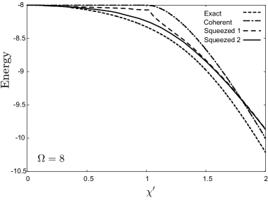
Fig. 1: Energy expectation values with respect to the squeezed state $|{\psi}\rangle$ by using Method 1 (dashed curve), Method 2 (solid curve) and the coherent state $|{\phi}\rangle$ (dash-dotted curve) are depicted together with the exact eigenvalues (dotted curve) in the case $\mathchar 28938\relax=8$. The horizontal axis represents $\chi^{\prime}$.

One way, which we call Method 1, is as follows: First, we set up phase factors as $\varphi_{X}=\varphi_{Y}=0$ because of the condition of energy minimum. Then, we determine the action variable $n_{X}$ from the condition $\partial\langle\hat{H}\rangle_{sq}/\partial n_{X}=0$. After that, from the minimum uncertain relation

$$(\mathchar 28929\relax\hat{Q})^{2}_{sq}(\mathchar 28929\relax\hat{P})^{2}_{sq}=\frac{\hbar^{2}}{4}|\langle\hat{R}\rangle_{sq}|^{2}\ ,$$ (5.3)

we determine the $n_{Y}$. Above-mentioned calculations should be carried out consistently. By using these variables, the energy expectation value can be estimated.

Another way, which we call Method 2, is as follows : First, we set up phase factor as $\varphi_{X}=\varphi_{Y}=0$ as well as the former way. Secondly, we determine the $n_{Y}$ from the minimum uncertain relation (5.3). After that, we seek the minimum energy expectation value with respect to $n_{X}$. In this case, $n_{X}$ which satisfies the condition $\partial\langle\hat{H}\rangle_{sq}/\partial n_{X}=0$ does not realize the energy minimum.

In Fig. 1, the energy expectation values obtained from Method 1 (dashed curve) and Method 2 (solid curve) are depicted compared with the exact ground state energy eigenvalues (dotted curve) with $\mathchar 28938\relax=8$ and $\epsilon=1$. The horizontal axis represents $\chi^{\prime}$ and the vertical axis represents the energy. The expectation value with respect to $|{\psi}\rangle$ is close to the exact energy eigenvalue compared with the usual Slater determinant approach (dash-dotted curve). Especially, near the phase transition point, $\chi^{\prime}=1$, the energy expectation values obtained by the squeezed state approach can trace the the exact energy eigenvalues approximately. It is pointed out, especially, that the energy expectation values near the transition point are well reproduced under the fixed minimum uncertainty relation (Method 2).

6 Summary

We have shown that an idea to extend the TDHF theory in the canonical form could be formulated based on the use of the state extended from the Slater determinant. The essential ingredients are to use the extended state from the Slater determinant and to impose the canonicity conditions. This extended state, which we call a quasi-spin squeezed state in the Lipkin model in our previous papers[6, 7] was a kind of the squeezed state in comparison with the $su(2)$-coherent state. This state was constructed similar to the usual boson squeezed state. By imposing the canonicity conditions for the variables which characterizes the coherent part and the squeezed part, we could obtain the sets of canonical variables. Thus, it becomes possible to formulate the extended TDHF theory as a canonical form.

As an application, the zero-point fluctuation induced by the uncertainty principle was investigated and the ground state energy was evaluated. It has been shown that the ground state energy is well reproduced compared with the results obtained by using the Slater determinant. Especially, it was shown that, near the transition point, the energy expectation values calculated by imposing the condition of the fixed minimum uncertainty relation have reproduced well the exact energy eigenvalues.

The dynamics will be investigated in our extended TDHF theory. This is a future problem.[11]

References

[1]
See, for example, P.Ring and P.Schuck, The Nuclear Many-Body Problem,
Springer-Verlag, (1980).
[2]
M. Yamamura and A. Kuriyama, Prog. Theor. Phys. Suppl. No. 93 (1987), 1.
[3]
T. Marumori, T. Maskawa, F. Sakata and A. Kuriyama, Prog. Theor. Phys.
64 (1980), 1294.
[4]
Y. Tsue, Y. Fujiwara, A. Kuriyama and M. Yamamura, Prog. Theor. Phys.
85 (1991), 693.
[5]
A. Kuriyama, J. da Providência, Y. Tsue and M. Yamamura,
Prog. Theor. Phys. Suppl. No.141 (2001), 113.
[6]Y. Tsue, A. Kuriyama and M. Yamamura, Prog. Theor. Phys.
92 (1994), 545.
[7]Y. Tsue, N. Azuma, A. Kuriyama and M. Yamamura,
Prog. Theor. Phys.
96 (1996), 729.
[8]
Y. Tsue, N. Azuma, A. Kuriyama and M. Yamamura,
NASA Conference Publication, NASA/CP-1998-206855 (1998), 221.
[9]
A. Kuriyama, M. Yamamura, C. Providência, J. da Providência and
Y. Tsue, J. of Phys. A36 (2003), 10361.
[10]
M. Yamamura, private communication (unpublished work).
[11]
H. Akaike, Y. Tsue and S. Nishiyama, submitted to Prog. Theor. Phys.