Observable implications of geometrical and dynamical aspects of freeze-out in heavy ion collisions

Abstract

Using an analytical parameterization of hadronic freeze-out in relativistic heavy ion collisions, we present a detailed study of the connections between features of the freeze-out configuration and physical observables. We focus especially on anisotropic freeze-out configurations (expected in general for collisions at finite impact parameter), azimuthally-sensitive HBT interferometry, and final-state interactions between non-identical particles. Model calculations are compared with data taken in the first year of running at RHIC; while not perfect, good agreement is found, raising the hope that a consistent understanding of the full freeze-out scenario at RHIC is possible, an important first step towards understanding the physics of the system prior to freeze-out.

I Introduction

The first data from collisions between heavy nuclei at the Relativistic Heavy Ion Collider (RHIC) have generated intense theoretical efforts to understand the hot, dense matter generated in the early stage of the collision QMconferences . Testing these theoretical ideas relies on comparison to experimental observables. Leptonic leptonicObservables or electromagnetic gammaProbes observables are believed to probe directly the early, dense stage of the collision. Most of the early data from RHIC, however, have been on hadronic observables. Measurements of hadrons at high transverse momentum ($p_{T}$) highpTexp have generated much excitement, as they may provide useful probes of the dense medium produced at RHIC highpTtheory . However, the medium itself decays largely into the soft (low-$p_{T}$) hadronic sector.

Soft hadronic observables measure directly the final “freeze-out” stage of the collision, when hadrons decouple from the bulk and free-stream to the detectors. Freeze-out may correspond to a complex configuration in the combined coordinate-momentum space, with collective components (often called “flow”) generating space-momentum correlations, as well as geometrical and dynamical (flow) anisotropies. A detailed experimental-driven understanding of the freeze-out configuration is the crucial first step in understanding the system’s prior evolution and the physics of hot colored matter.

In this paper, we explore in detail an analytic parameterization of the freeze-out configuration, which includes non-trivial correlations between coordinate- and momentum-space variables. We discuss the connections between the physical parameters of the model and observable quantities. If the model, with correct choice of physical model parameters, can adequately reproduce several independent measured quantities, then it might be claimed that this “crucial first step,” mentioned above, has been performed.

A consistent reproduction of all low-$p_{T}$ observations at RHIC is not achieved in most physical models which aim to describe the evolution of the collision. In particular, it is difficult to reproduce momentum-space measurements while simultaneously describing the freeze-out coordinate-space distribution probed by two-particle intensity interferometry measurements WH99 (also known as Hanburry-Brown-Twiss or HBT HanburryBrownTwiss measurements). Hadronic cascade models predict a too weak momentum azimuthal anisotropy and too large source sizes CascadeFail . Hydrodynamic transport models describe successfully transverse mass spectra and elliptic flow but fail at describing pion source radii HK01 ; some hydrodynamic models have successfully reproduced pion source radii Hirano_HBT , but only with different model parameters than those used to reproduce spectra and elliptic flow Hirano_SpectraV2 . Similarly, sophisticated hybrid transport models (e.g. AMPT AMPT ) require different model parameters ZiWei to reproduce data on elliptic flow AMPTv2 and HBT AMPT_HBT . Good reproduction of observed values has been acheived in models which adjust parameters to fit data within a given freeze-out scenario, such as in the Buda-Lund hydro approach BudaLund . The work presented here falls into this latter category.

The parameterization used in this paper (“blast-wave parameterization”) is similar in form to the freeze-out configuration obtained from hydrodynamic calculations HKHRV01 , but we treat the physical parameters of the configuration (e.g. temperature) as free parameters. Our main goal is simply to quantify the driving physical parameters of freeze-out at RHIC, and the dependence of observables on these parameters.

Further motivation for exploring freeze-out configurations of the type discussed here, is that they implicitly assume a “bulk” system which may be described by global parameters (temperature, flow strength, etc). Discussions of a “new phase of matter” and its “Equation of State” are only sensible if indeed such assumptions hold. Comparison of blast-wave calculations with several independent measurements, then, is a crucial consistency check of these assumptions (though, of course, a successful comparison still would not constitute a proof of their validity).

In transport models, whether the constituents are hadrons RQMD ; Humanic , partons MolnarPC ; BassPC , or fluid elements HK01 ; HK02 ; TLS01 ; TeaneyViscosity , if they re-interact substantially, pressure gradients are generated, leading to collective velocity fields (“flow”), pushing the matter away from the hot center of the collision and into the surrounding vacuum. Evidence of collective flow, generated by final state re-interaction of collision products, has been based largely on interpretations of transverse mass spectra and transverse momentum azimuthal anisotropy HK01 . However, this scenario has been challenged by new measurements of p-Au collisions NA49Fischer and new theoretical interpretations ColorGlassCond . Indeed, so-called initial state effects such as random walk of the incoming nucleons NA49Fischer or Color Glass Condensate phenomena ColorGlassCond may offer an alternative explanation of the measured spectra and anisotropies in transverse momentum. This ambiguity apparently threatens the concept that a bulk system has been created at all. However, it is important to recall that collective expansion, if it exists, would manifest itself not only in momentum-space observables, but would also generate space-momentum correlations, which can be measured via two-particle correlations.

The possible validity of any scenario may only be claimed if a single set of model parameters allows a successful description of all measured observables. Here, we study, in the context of a bulk collective flow scenario, transverse momentum spectra, momentum-space anisotropy (“elliptic flow”), HBT interferometry, and correlations between non-identical particles.

Similar studies have been reported previously TeaneyViscosity ; PeitzmannBWHighPt ; BurwardHoy ; Peitzmann ; Tomasik . New aspects in our study include: consideration of a more general (azimuthally-anisotropic) freeze-out configuration, applicable to non-zero impact parameters; model studies of azimuthally-sensitive HBT interferometry and correlations between non-identical particles; and a multi-observable global fit to several pieces of published RHIC data.

This paper is organized as follows: In Section II, we describe the blast-wave parameterization. In Section III, we investigate in detail the sensitivity of several observables ($p_{T}$ spectra, elliptic flow, pion HBT radii, and average space-time separation between different particle types) on the physical parameters of the blast-wave parameterization. In Section IV, we perform fits to published data measured at RHIC for Au+Au collisions at $\sqrt{s_{NN}}=130$ GeV, and, based on these fits, describe how as-yet unpublished analyses (azimuthally-sensitive HBT interferometry, and correlations between non-identical particles) are expected to look. The reader primarily interested in the quality of the fit to the data and the resulting parameters may want to skip past the details of Section III. In Section V, we summarize and conclude on the relevance of the blast-wave parameterization at RHIC.

II The blast-wave Parameterization

II.1 Geneology and Motivation

More than a quarter of a century ago, Westfall et al Westfall76 introduced the nuclear fireball model to explain midrapidity proton spectra. The idea was that the overlapping nucleons of the target and projectile combined to create a hot source with velocity between that of the target and projectile. Protons emitted from this source were expected to be emitted isotropically with a thermal energy distribution.

Soon thereafter, Bondorf, Garpman, and Zimanyi BGZ78 derived a non-relativistic expression for the energy spectra of particles emitted from a thermal exploding source. The radial flow in their (spherical) source results in energy spectra increasingly different than those from a purely thermal (non-flowing) source, as the particle mass increases. Siemens and Rasmussen SR79 then generalized the formula with relativistic kinematics, further simplifying by assuming a single expanding radial shell.

While a spherically-expanding source may be expected to approximate the fireball created in lower-energy collisions, at higher energies stronger longitudinal flow may lead to a cylindrical geometry. A decade ago, Schnedermann et al SSH93 introduced a simple functional form for the phasespace density at kinetic freezeout, which approximated hydrodynamical results assuming boost-invariant longitudinal flow BjorkenBI , and successfully used it to fit $p_{T}$ spectra with only two parameters: a kinetic temperature, and a radial flow strength. The coordinate space geometry was an infinitely long solid cylinder (and so should approximate the situation for $b=0$ collisions at midrapidity); the transverse radial flow strength necessarily vanished along the central axis, and is assumed maximum at the radial edge. Most hydrodynamic calculations yield a transverse rapidity flow field linear in the radial coordinate TLS01 .

Huovinen et al HKHRV01 generalized this parameterization to account for the transversely anisotropic flow field which arises in non-central collisions, and which generates an elliptic flow signal similar to that seen in measurements STARv2ID . This added one more parameter– the difference between the flow strength in, and out of, the reaction plane. The spatial geometry remained cylindrical, though it was assumed to be a cylindrical shell, not a solid cylinder.

The measured elliptical flow systematics as a function of $p_{T}$ and mass are fairly well-fit with the Huovinen parameterization STARv2ID . However, better fits were achieved when the STAR Collaboration generalized the model even further, adding a fourth parameter designed to account for the anisotropic shape of the source in coordinate space STARv2ID . A shell geometry was still assumed.

To calculate the spatial homogeneity lengths probed by two-particle correlation measurements WH99 , we must revert from the unrealistic shell geometry to a solid emission region (infinite series of elliptical shells). Furthermore, additional parameters corresponding to the source size, emission time, and emission duration must be included, increasing the number of parameters FabriceBW . A similar generalization has been studied by Wiedemann W98 . Finally, in this paper, we explore the effects of a “hard-edge” versus a smooth spatial density profile; similar studies have recently been done by Tomás̆ik et al Tomasik9901 and Peitzmann Peitzmann for the more restricted case of a transversely-isotropic source. This brings to eight the total number of parameters which we study.

Although the blast-wave functional form was motivated by its similarity to the freeze-out configuration of a real dynamical model (i.e. hydrodynamical solutions), it is not necessarily true that the hydrodynamical freeze-out configuration corresponds to the parameter set that best describes the data. In this sense, the blast-wave model presented here remains only a parameterization. With eight freely-tunable parameters, it is clearly a toy model with little predictive power. However, the goal is to see whether a consistent description of the data from the soft sector at RHIC is possible within a simple boost-invariant model with transverse collective flow. If this turns out to be the case, then it is worthwhile considering that the parameter values indeed characterize the size, shape, timescales, temperature, and flow strengths of the freeze-out configuration. A consistent parameterization in terms of such physical quantities represents a true step forward, and provides valuable feedback to theorists constructing physical models of the collision.

II.2 Parameters and Quantities in the blast-wave

The eight parameters of the blast-wave parameterization described in this paper are $T$, $\rho_{0}$, $\rho_{2}$, $R_{y}$, $R_{x}$, $a_{s}$, $\tau_{0}$, and $\Delta\tau$; their physical meaning is given below.

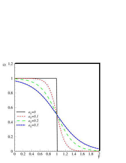
Figure 1: (Color online) The source weighting function $\Omega$, as a function of the normalized elliptical radius $\tilde{r}$ for several values of the surface diffuseness parameter $a_{s}$.

The freeze-out distribution is infinite in the beam ($z$) direction, and elliptical in the transverse ($x-y$) plane. (The $x-z$ plane is the reaction plane.) The transverse shape is controlled by the radii $R_{y}$ and $R_{x}$, and the spatial weighting of source elements is given by

$$\Omega(r,\phi_{s})=\Omega(\tilde{r})=\frac{1}{1+e^{(\tilde{r}-1)/a_{s}}}$$ (1)

where a fixed value of the “normalized elliptical radius”

$$\tilde{r}(r,\phi_{s})\equiv\sqrt{\frac{(r\cos(\phi_{s}))^{2}}{R_{x}^{2}}+\frac{(r\sin(\phi_{s}))^{2}}{R_{y}^{2}}}$$ (2)

corresponds to a given elliptical sub-shell within the solid volume of the freeze-out distribution.

The parameter $a_{s}$ corresponds to a surface diffuseness of the emission source. As shown in Figure 1, a hard edge (“box profile”) may be assumed by setting $a_{s}=0$, while the density profile approximates a Gaussian shape for $a_{s}\approx 0.3$.

It should be noted that the weighting function $\Omega(r,\phi_{s})$ is not, in general, the source density distribution. In particular, as we discuss especially in Sections III.3 and III.4, non-zero collective flow induces space-momentum correlations which dominate the spatial source density distributions. Only for a system without flow ($\rho_{0}=\rho_{2}=0$, see below), the source distribution is given by $\Omega$, so that, e.g., for $a_{s}=0$, there is a uniform density of sources ($\frac{d^{2}N}{dxdy}={\rm const}$) inside the ellipse defined by $R_{y}$ and $R_{x}$, and no sources outside.

The momentum spectrum of particles emitted from a source element at $(x,y,z)$ is given by a fixed temperature $T$ describing the thermal kinetic motion, boosted by a transverse rapidity $\rho(x,y)$. This is common in models of this type. However, unlike transversely isotropic parameterizations, the azimuthal direction of the boost (denoted $\phi_{b}$) is not necessarily identical to the spatial azimuthal angle $\phi_{s}=\tan^{-1}(y/x)$. Instead, in our model, the boost is perpendicular to the elliptical sub-shell on which the source element is found; see Figure 2. We believe this to be a more natural extension of an “outward” boost for non-isotropic source distributions than that used by Heinz and Wong HW02 , who used an anisotropic shape but always assumed radial boost direction ($\phi_{b}=\phi_{s}$). It may be shown that for our model

$$\tan(\phi_{s})=\left(\frac{R_{y}}{R_{x}}\right)^{2}\tan(\phi_{b}).$$ (3)

Figure 2: Schematic illustration of an elliptical sub-shell of the source. Here, the source is extended out of the reaction plane ($R_{y}>R_{x}$). Arrows represent the direction and magnitude of the flow boost. In this example, $\rho_{2}>0$ (see Equation 4).

Hydrodynamical calculations for central collisions (i.e. azimuthally isotropic freezeout distribution) suggest that the flow rapidity boost depends linearly on the freeze-out radius TLS01 . We assume a similar scenario, but in our more generalized parameterization, the boost strength depends linearly on the normalized elliptical radius $\tilde{r}$ defined in Equation 2. Thus, in the absence of an azimuthal dependence of the flow (to be introduced shortly), all source elements on the outer edge of the source boost with the same (maximum) transverse rapidity $\rho_{0}$ in an “outward” direction.

In non-central collisions, the strength of the flow boost itself may depend on azimuthal angle, as suggested by Huovinen et al HKHRV01 . As those authors did, we incorporate this via a parameter $\rho_{2}$, which characterizes the strength of the second-order oscillation of the transverse rapidity as a function of $\phi_{b}$. Hence, the flow rapidity is given by

$$\rho(r,\phi_{s})=\tilde{r}\left(\rho_{0}+\rho_{2}\cos(2\phi_{b})\right).$$ (4)

We note that source anisotropy enters into our parameterization in two independent ways, and each contributes to, e.g., elliptic flow. Setting $\rho_{2}>0$ means the boost is stronger in-plane than out-of-plane, contributing to positive elliptic flow. However, even if $\rho_{2}=0$ (but $\rho_{0}\neq 0$), setting $R_{y}>R_{x}$ still generates positive elliptic flow, since this means there are more sources emitting in-plane than out-of-plane (see Figure 2). The STAR Collaboration found that both types of anisotropy were required to fit their elliptic flow data STARv2ID . In generalizing the circular transverse geometry parameterization of Huovinen et al HKHRV01 (in which $\phi_{b}=\phi_{s}$), they added a parameter $s_{2}$ and weighted source elements with a given $\phi_{b}$ as

$$\frac{dN}{d\phi_{b}}=\frac{dN}{d\phi_{s}}\sim(1+2s_{2}\cos(2\phi_{s}))$$ (5)

Thus, a positive value of $s_{2}=\langle\cos(2\phi_{b})\rangle$ corresponded to more source elements emitting in-plane, similar to setting $R_{y}>R_{x}$ in our parameterization.

To facilitate comparison of fits with the STAR model and with ours, we relate the $s_{2}$ of STAR to the geometric anisotropy of our parameterization. In the case of isotropic boost ($\rho_{2}=0$) thanksSergeiVoloshin ,

$$s_{2}=\langle\cos(2\phi_{b})\rangle=\frac{1}{2}\frac{\left(\frac{R_{y}}{R_{x}}\right)^{2}-1}{\left(\frac{R_{y}}{R_{x}}\right)^{2}+1}.$$ (6)

If $\rho_{2}\neq 0$, anisotropies in the space-momentum correlations lead to a significantly more complicated expression.

Finally, since our model is based on a longitudinally boost-invariant assumption, it is sensible that the freezeout occurs with a given distribution in longitudinal proper time $\tau=\sqrt{t^{2}-z^{2}}$. We assume a Gaussian distribution peaked at $\tau_{0}$ and with a width $\Delta\tau$

$$\frac{dN}{d\tau}\sim\exp\left(-\frac{(\tau-\tau_{0})^{2}}{2\Delta\tau^{2}}\right).$$ (7)

We note that although the source emits particles over a finite duration in proper time $\tau$, we assume that none of the source parameters changes with $\tau$. This is obviously an oversimplification valid only for small $\Delta\tau$; with time, one may expect the flow field to evolve (increase or decrease), and it is natural to expect the transverse sizes $R_{x}$ and $R_{y}$ to change (grow or fall) with time. However, calculation of the time dependence of these parameters requires a true dynamical model and is outside the scope and spirit of the present work.

II.3 The Emission Function

Our emission function is essentially a generalization of azimuthally-isotropic emission functions used by previous authors AS95 ; WSH96 ; CL96 ; WHTW98 , and here we follow closely WSH96 :

$$S(x,K) = m_{T}\cosh(\eta-Y)\Omega(r,\phi_{s})e^{\frac{-(\tau-\tau_{0})^{2}}{2\Delta\tau^{2}}}\times$$

$$\frac{1}{e^{K\cdot u/T}\pm 1}$$

$$= m_{T}\cosh(\eta-Y)\Omega(r,\phi_{s})e^{\frac{-(\tau-\tau_{0})^{2}}{2\Delta\tau^{2}}}\times$$

$$\sum_{n=1}^{\infty}(\mp 1)^{n+1}e^{-nK\cdot u/T}.$$

Where the upper (lower) sign is for fermions (bosons). Often, only the first term in the sum in Equation II.3 is used, resulting in a Boltzmann distribution for all particles. Below, we show that there is a small change to observables when truncating after the second term, and negligible effect when including further terms. The Boltzmann factor $\exp(-K\cdot u/T)$ arises from our assumption of local thermal equilibrium within a source moving with four-velocity $u_{\mu}(x)$. We assume longitudinal boost invariance by setting the longitudinal flow velocity $v_{L}=z/t$ ($z=\tau\sinh\eta$ and $t=\tau\cosh\eta$), so that the longitudinal flow rapidity $\eta_{\rm flow}=\frac{1}{2}\ln\left[(1+v_{L})/(1-v_{L})\right]$ is identical BjorkenBI to the space-time rapidity $\eta=\frac{1}{2}\ln\left[(t+z)/(t-z)\right]$. Thus, in cylindrical coordinates

$$u_{\mu}(x)=\left(\cosh\eta\cosh\rho(r,\phi_{s}),\sinh\rho(r,\phi_{s})\cos\phi_{b},\right.$$

$$\left.\sinh\rho(r,\phi_{s})\sin\phi_{b},\sinh\eta\cosh\rho(r,\phi_{s})\right)$$ (9)

and

$$K_{\mu}=\left(m_{T}\cosh Y,p_{T}\cos\phi_{p},p_{T}\sin\phi_{p},m_{T}\sinh Y\right),$$ (10)

where the transverse momentum ($p_{T}$), transverse mass ($m_{T}$), rapidity ($Y$), and azimuthal angle ($\phi_{p}$) refer to the momentum of the emitted particle, not the source element. (Note that three azimuthal angles– $\phi_{s}$, $\phi_{b}$, and $\phi_{p}$– are relevant to this discussion.) Thus

$$K_{\mu}u^{\mu}=m_{T}\cosh\rho(r,\phi_{s})\cosh(\eta-Y)-$$

$$p_{T}\sinh\rho(r,\phi_{s})\cos(\phi_{b}-\phi_{p}),$$ (11)

and the emission function (Equation II.3) may be rewritten as

$$S(x,K) = S(r,\phi_{s},\tau,\eta)$$

$$= m_{T}\cosh(\eta-Y)\Omega(r,\phi_{s})e^{\frac{-(\tau-\tau_{0})^{2}}{2\Delta\tau^{2}}}\times$$

$$\sum_{n=1}^{\infty}(\mp 1)^{n+1}e^{n\alpha\cos(\phi_{b}-\phi_{p})}e^{-n\beta\cosh(\eta-Y)}.$$

where we define

$$\alpha\equiv\frac{p_{T}}{T}\sinh\rho(r,\phi_{s})$$ (13)

$$\beta\equiv\frac{m_{T}}{T}\cosh\rho(r,\phi_{s}).$$ (14)

Exploiting the boost invariance and infinite longitudinal extension of our source, and focusing on observables at midrapidity and using the longitudinally co-moving system (LCMS) for HBT measurements, we may simplify Equation II.3 by setting $Y=0$.

II.4 Calculating Observables

All observables which we will calculate are related to integrals of the emission function (II.3) over phasespace $d^{4}x=dxdydzdt=\tau d\tau d\eta rdrd\phi_{s}$, weighted with some quantity $B(x,K)$. In all cases, the integrals over $\tau$ and $\eta$ may be done analytically, though the result depends on whether $B(x,K)$ itself depends on $\tau$ and $\eta$.

In particular, if $B(x,K)=B^{\prime}(r,\phi_{s},K)\tau^{i}\sinh^{j}\eta\cosh^{k}\eta$ then the integrals of interest are caviat

$$\int_{0}^{2\pi}d\phi_{s}\int_{0}^{\infty}rdr\int_{-\infty}^{\infty}d\eta\int_{-\infty}^{\infty}\tau d\tau S(x,K)B(x,K)$$

$$=m_{T}H_{i}\cdot\left\{B^{\prime}\right\}_{j,k}(K)$$ (15)

where the $\tau$ and $\eta$ integrals are denoted

$$H_{i} \equiv \int_{-\infty}^{\infty}d\tau\tau^{i+1}e^{\frac{-(\tau-\tau_{0})^{2}}{2\Delta\tau^{2}}}$$

$$H_{0} = \sqrt{2\pi}\cdot\Delta\tau\cdot\tau_{0}$$

$$H_{1} = \sqrt{2\pi}\cdot\Delta\tau\cdot\left(\Delta\tau^{2}+\tau_{0}^{2}\right)$$ (16)

$$H_{2} = \sqrt{2\pi}\cdot\Delta\tau\cdot\tau_{0}\left(3\Delta\tau^{2}+\tau_{0}^{2}\right)$$

and

$$G_{j,k}(x,K) \equiv \int_{-\infty}^{\infty}d\eta e^{-\beta\cosh\eta}\sinh^{j}\eta\cosh^{k+1}\eta$$

$$G_{0,0}(x,K) = 2{\rm K}_{1}(\beta)$$

$$G_{0,1}(x,K) = 2\left[\frac{{\rm K}_{1}(\beta)}{\beta}+{\rm K}_{0}(\beta)\right]$$

$$G_{1,0}(x,K) = G_{1,1}(x,K)=0$$ (17)

$$G_{0,2}(x,K) = 2\left[\frac{{\rm K}_{2}(\beta)}{\beta}+{\rm K}_{1}(\beta)\right]$$

$$G_{2,0}(x,K) = 2\frac{{\rm K}_{2}(\beta)}{\beta}.$$

$\beta$ was defined in (14), and $\rm{K}_{n}$ are the modified Bessel functions. For the above, we define the notation

$$\left\{B^{\prime}\right\}_{j,k}(K)\equiv\sum_{n=1}^{\infty}\left\{(\mp 1)^{n+1}\int_{0}^{2\pi}d\phi_{s}\int_{0}^{\infty}rdr\left[\right.\right.$$

$$\left.\left.G_{j,k}(x,nK)B^{\prime}(x,K)\times e^{n\alpha\cos(\phi_{b}-\phi_{p})}\Omega(r,\phi_{s})\right]\right\}$$ (18)

for the remaining integrals, which we perform numerically. (Note that $G_{i,j}(x,nK)$ retains dependence on $r$ and $\phi_{s}$ due to its dependence on $\beta$, as defined in Equation 14, and so cannot move outside the integrals in Equation 18.)

III Calculation of Hadronic Observables

In this Section, we discuss how hadronic observables are calculated from the parameterized source and illustrate the sensitivity of these observables to the various parameters presented in Section II.2.

With several observables depending on several parameters, it is not feasible to explore the entire numerical parameter space. Instead, we anticipate the results of the next Section, in which we fit our model to existing data, and vary the parameters by “reasonable” amounts about values similar to those which fit the data. The default parameter values used in several of the calculations in this Section are listed in Table 1.

parameter	round source	non-round source
$\rho_{2}$	0	0.05
$R_{x}$ (fm)	12.04	11
$R_{y}$ (fm)	12.04	13
$T$ (GeV)	0.1
$\rho_{0}$	0.9
$\tau_{0}$ (fm/c)	9
$\Delta\tau$ (fm/c)	2
$a_{s}$	0

Table 1: Default parameter values for most calculations in Section III. Note that $\rho_{2}$, $R_{x}$ and $R_{y}$ default values depend on whether we are discussing an azimuthally isotropic (“round”) or anisotropic (“non-round”) source. One might expect such sources from central and peripheral collisions, respectively.

III.1 $p_{T}$ spectra

In the notation of Section II.4 the (azimuthally-integrated) $p_{T}$ spectrum is calculated as

$$\frac{dN}{p_{T}dp_{T}} = \int d\phi_{p}\int d^{4}xS(x,K)$$ (19)

$$\propto m_{T}\int d\phi_{p}\left\{1\right\}_{0,0}(K).$$

In this paper, we focus only on the shapes, not the normalizations, of the spectra.

We note that spectra calculated in the blast-wave model scale neither with $m_{T}$ nor $p_{T}$, as both quantities enter the expression through $\alpha$ and $\beta$ (Equations (13) and (14)). This breaking of $m_{T}$-scaling is a well-known consequence of finite transverse flow SSH93 ($\rho\neq 0$ in our model).

According to Equation 19, $m_{T}$ spectra calculated in the blast-wave model are insensitive to the time parameters $\tau_{0}$ and $\Delta\tau$. The spectral shapes are furthermore insensitive to the spatial scale (i.e. $R_{y}$) of the source, though, as we see below, there is some small sensitivity to the spatial shape (i.e. $\frac{R_{y}}{R_{x}}$).

First, we study the importance of using quantum (as opposed to classical) statistics in the source function. Figure 3 shows $p_{T}$ spectra for pions and protons, treated as bosons and fermions, respectively. Model parameters were set to the “non-round” values listed in Table 1. The sum in Equation II.3 (and Equations II.3 and 18) is over $n=1\ldots N$; curves are shown for $N=1,2,3,4$. For parameter values in the range we study here, proton spectra are essentially independent of $N$. For $N>1$, the pion spectra are likewise robust against the value of $N$, though in the classical limit ($N=1$), there is relatively lower yield at low $p_{T}$. (Note that all spectra are arbitrarily normalized to unity at $p_{T}=0$.) Calculations below use the truncation $N=2$.

Figure 3: Transverse momentum spectra for protons (upper curves) and pions (lower curves), as calculated by Equation 19, for several values of $N$, the maximum value of $n$ taken in the summation of Equation II.3; see text for details. Parameters values correspond to the “non-round” source of Table 1. All spectra are arbitrarily normalized to unity at $p_{T}=0$.

III.1.1 Spectra from Central Collisions

Focusing first on central collisions (so that the flow anisotropy parameter $\rho_{2}=0$ and $R_{x}=R_{y}$), then, we need only consider the spectra sensitivity to the temperature and radial flow parameters $\rho_{0}$ and $T$, and to the surface diffusion $a_{s}$.

Fixing the transverse spatial density distribution to a box profile ($a_{s}=0$), the evolution of spectral shapes for pions and protons are shown in Figures 4 and 5, as the temperature and radial flow parameter, respectively, are varied about nominal values of $T=100$ MeV and $\rho_{0}=0.9$. As has been noted previously SSH93 , at low $p_{T}$, temperature variations affect the lighter pions more strongly, while variations in the collective flow boost produce a stronger effect on the heavier particles.

Figure 4: Transverse momentum spectra for protons (upper curves) and pions (lower curves), as calculated by Equation 19, for several values of the temperature parameter $T$. Other parameters follow the “round” source defaults of Table 1. All spectra are arbitrarily normalized to unity at $p_{T}=0$.

Figure 5: Transverse momentum spectra for protons (upper curves) and pions (lower curves), as calculated by Equation 19, for several values of the radial flow parameter $\rho_{0}$. Other parameters follow the “round” source defaults of Table 1. All spectra are arbitrarily normalized to unity at $p_{T}=0$.

Figure 6: The geometric constant of proportionality $F$ between the average transverse flow boost $\langle\rho\rangle$ and the blast-wave parameter $\rho_{0}$, as a function of the surface diffuseness $a_{s}$.

Figure 7: Transverse momentum spectra for protons (upper curves) and pions (lower curves), as calculated by Equation 19, for several values of the surface diffuseness parameter $a_{s}$. The radial flow strength $\rho_{0}$ is co-varied; see text for details. Other parameters follow the “round” source defaults of Table 1. All spectra are arbitrarily normalized to unity at $p_{T}=0$.

Next, we consider the effect of a finite surface diffuseness parameter ($a_{s}\neq 0$), i.e., using the smoother spatial density distributions of Figure 1. Since we assume a transverse flow profile which increases linearly with radius (c.f. Equation 4), one trivial effect is that, for a fixed $\rho_{0}$, increasing $a_{s}$ will produce a larger average flow boost $\langle\rho\rangle$. The effect of increasing transverse flow was already explored directly in Figure 5, so we avoid this trivial effect here, and explore the effect of varying $a_{s}$, while keeping $\langle\rho\rangle$ constant Peitzmann .

The average transverse flow boost $\langle\rho\rangle=F(a_{s})\cdot\rho_{0}$ where the geometric proportionality constant

$$F(a_{s})=\frac{\int_{0}^{\infty}dx\frac{x^{2}}{1+\exp((x-1)/a_{s})}}{\int_{0}^{\infty}dx\frac{x}{1+\exp((x-1)/a_{s})}}$$ (20)

is independent of $\rho_{0}$ or $R=R_{x}=R_{y}$. For the box profile, $F(a_{s}=0)=\frac{2}{3}$. Figure 7 shows this geometric factor as a function of the surface diffuseness.

Figure 7 shows the pion and proton spectra for various values of $a_{s}$. The radial flow strength $\rho_{0}$ was co-varied with $a_{s}$ so that the average transverse flow boost was $\langle\rho\rangle=0.6$. To a first approximation, the spectral shapes depend only on the temperature $T$ and the average transverse flow boost $\langle\rho\rangle$. The residual dependence on the surface diffuseness parameter $a_{s}$ arises from the fact that while the average boost rapidity has been held constant, the spread of boost rapidities increases with increasing $a_{s}$ Peitzmann . Thus, we observe qualitatively similar variations in the spectral shapes when $a_{s}$ increases (Figure 7), as when $T$ increases (Figure 4). The variations are not quantitatively identical since in the present case, the velocity spread is not thermal, and the particle velocity spread evolves differently with mass, depending on whether it arises from a boost spread or a thermal spread.

III.1.2 Dependence of spectral shapes on source anisotropy

Azimuthally-integrated $p_{T}$ spectra are often presented as a function of event centrality. For $b\neq 0$ collisions, the emitting source may have anisotropic structure ($R_{x}\neq R_{y}$ and $\rho_{2}\neq 0$ in the present model). Thus, it is interesting to explore possible effects of these anisotropies.

For an azimuthally isotropic flow field ($\rho_{2}=0$), the spectral shapes are insensitive to spatial anisotropies in the source (i.e. $R_{x}\neq R_{y}$). This is because the spectral shapes are determined by the distribution of boost velocities Peitzmann , which is unchanged by a shape change in our parameterization, if $\rho_{2}=0$.

For an azimuthally-symmetric spatial source ($R_{x}=R_{y}$), a very small variation in the $\phi_{p}$-integrated spectral shapes is observed when $\rho_{2}$ is changed from a value of 0.0 to 0.15, as seen in Figure 9. This, again, is due to the slightly increased spread in boost velocities; source elements emitting in-plane boost a bit more, and out-of-plane a bit less. This effect becomes stronger in the presence of an out-of-plane spatial anisotropy ($R_{y}/R_{x}>1$) as shown in Figure 9. In any case, the effects of “reasonable” source anisotropy on the shapes of azimuthally-integrated spectra are very small.

Figure 8: Transverse momentum spectra for protons (upper curves) and pions (lower curves), as calculated by Equation 19 for an azimuthally symmetric flow field ($\rho_{2}=0$) and an asymmetric field ($\rho_{2}=0.15$). Other parameters follow the “round” source defaults of Table 1. All spectra are arbitrarily normalized to unity at $p_{T}=0$.

Figure 9: Transverse momentum spectra for protons (upper curves) and pions (lower curves), as calculated by Equation 19 for an azimuthally anisotropic flow field ($\rho_{2}=0.15$), and a spatially isotropic ($R_{y}/R_{x}=1$) and anisotropic ($R_{y}/R_{x}=1.5$) spatial distribution. Other parameters follow the “round” source defaults of Table 1.

Thus, we conclude that azimuthally-integrated $p_{T}$ spectra are largely insensitive to “reasonable” source anisotropies (see Section IV for “reasonable” ranges) and probe mainly the thermal motion ($T$) and average transverse flow boost ($\langle\rho\rangle$) of the source.

III.2 Elliptic flow versus mass and $p_{T}$

In the notation of Section II.4 the elliptic flow parameter $v_{2}$ is calculated as

$$v_{2}(p_{T},m)=\frac{\int_{0}^{2\pi}d\phi_{p}\left\{\cos(2\phi_{p})\right\}_{0,0}(K)}{\int_{0}^{2\pi}d\phi_{p}\left\{1\right\}_{0,0}(K)}$$ (21)

A finite $v_{2}$ arises from azimuthal anisotropies in the source ($R_{x}\neq R_{y}$ and/or $\rho_{2}\neq 0$). As discussed below, however, the parameters $\rho_{0}$ and $T$ strongly affect its value and evolution with $p_{T}$ and mass. In the present parameterization, $v_{2}$ is not sensitive to the overall spatial scale of the source ($R_{y}$) or the time parameters $\tau_{0}$ and $\Delta\tau$.

The $v_{2}$ parameter depends non-trivially on both $p_{T}$ and particle mass VP00 ; HKHRV01 ; STARv2ID ; VoloshinQM03 . In this section, we explore the evolution of pion and proton $v_{2}$, as we vary the model parameters from nominal “non-round” values for non-central collisions (cf 1).

As with the $p_{T}$ spectra of Section III.1, we first check the importance of quantum statistics. Figure 10 shows $v_{2}$ for pions and protons, for different values of $N$, where the sum in Equation II.3 (and Equations II.3 and 18) runs over $n=1\ldots N$. Again, we find only a small difference for the pions between $N=1$ (classical limit) and $N=2$, beyond which $v_{2}$ is robust against further increases in $N$. Calculations here use $N=2$.

Figure 10: Elliptic flow parameter $v_{2}$ for pions (upper curves) and protons (lower curves), as a function of transverse momentum, as calculated by Equation 21, for several values of $N$, the maximum value of $n$ taken in the summation of Equation II.3; see text for details. Model parameters follow the “non-round” source defaults of Table 1.

Figure 11: Elliptic flow parameter $v_{2}$ for pions (upper curves) and protons (lower curves), as a function of transverse momentum, as calculated by Equation 21, for various values of the temperature parameter $T$. Other parameters follow the “non-round” source defaults of Table 1.

Figure 11 shows the evolution of $v_{2}$ as the temperature parameter ($T$) is varied. For both particle types shown, the increased thermal smearing in momentum space, as $T$ is increased, leads to a reduced momentum-space anisotropy. The effect of the thermal smearing is greater for the lighter pions.

Figure 12: Elliptic flow parameter $v_{2}$ for pions (upper curves) and protons (lower curves), as a function of transverse momentum, as calculated by Equation 21, for various values of the transverse flow parameter $\rho_{0}$. The source spatial distribution is assumed azimuthally-anisotropic ($R_{y}=R_{x}$), but other parameters follow the “non-round” source defaults of Table 1.

Figure 13: Elliptic flow parameter $v_{2}$ for pions (upper curves) and protons (lower curves), as a function of transverse momentum, as calculated by Equation 21, for various values of the transverse flow parameter $\rho_{0}$. Other parameters follow the “non-round” source defaults of Table 1.

Less intuitive is the evolution of $v_{2}$ as the flow field ($\rho_{0}$ or $\rho_{2}$) is varied. In Figures 12 and 13, the average transverse flow parameter $\rho_{0}$ is varied for an azimuthally isotropic ($R_{y}/R_{x}=1$) and anisotropic ($R_{y}/R_{x}=13/11$) shape, respectively. For the isotropic spatial distribution, we find that $v_{2}$ decreases as $\rho_{0}$ increases, for all $p_{T}$ and for both particle types. This is due to the decreasing relative amplitude of the oscillation in the flow field. Not surprisingly, the effect is larger for the heavier protons.

Figure 14: Elliptic flow parameter $v_{2}$ for pions (upper curves) and protons (lower curves), as a function of transverse momentum, as calculated by Equation 21, for various values of the modulation in the transverse flow $\rho_{2}$. Other parameters follow the “round” (note: $R_{y}=R_{x}$) source defaults of Table 1.

Figure 15: Elliptic flow parameter $v_{2}$ for pions (upper curves) and protons (lower curves), as a function of transverse momentum, as calculated by Equation 21, for various values of the modulation in the transverse flow $\rho_{2}$. Other parameters follow the “non-round” source defaults of Table 1.

Indeed, it has been pointed out Voloshin97 ; HKHRV01 ; VoloshinQM03 that high radial flow (large $\rho_{0}$) can lead to negative values of $v_{2}$ for heavy particles; this is clearly true for the protons in Figure 12. This negative $v_{2}$ reflects the depletion of the low-$p_{T}$ particle yield when most source elements are highly boosted transversely; this is also the origin of the “shoulder arm” in the $p_{T}$ spectra (c.f. Section III.1). This depletion is larger in-plane (since the boost is higher, i.e. $\rho_{2}>0$), leading to negative $v_{2}$. At higher $p_{T}$, and/or lower flow strengths, the competing effect is dominant: the larger in-plane boost leads to more particles emitted in-plane, and $v_{2}>0$.

For a slightly anisotropic shape ($R_{y}/R_{x}=13/11$; Figure 13), the $v_{2}$ parameter increases significantly for both protons and pions, due to the larger number of source elements boosted in-plane (c.f. Figure 2). The finite spatial asymmetry leads to an effect that tends to oppose the reduction of $v_{2}$ with increasing $\rho_{0}$, discussed above, and, for pions at low $p_{T}$, even reverses it in this case. Hence, at low $p_{T}$, increasing $\rho_{0}$ increases (decreases) $v_{2}$ for pions (protons).

We observe similar trends when $\rho_{0}$ is held fixed, and $\rho_{2}$ is varied. Figure 14 shows $v_{2}$ evolution for a spatially azimuthally-symmetric source ($R_{y}/R_{x}=1$) and Figure 15 for a slightly asymmetric source ($R_{y}/R_{x}=13/11$).

Figure 16: Elliptic flow parameter $v_{2}$ for pions (upper curves) and protons (lower curves), as a function of transverse momentum, as calculated by Equation 21, for various values of the spatial anisotropy ($R_{y}/R_{x}$). Elliptic flow parameter $v_{2}$ for pions (upper curves) and protons (lower curves), as a function of transverse momentum, as calculated by Equation 21, for various values of the modulation in the transverse flow $\rho_{2}$. Other parameters follow the “round” (note: $\rho_{2}=0$) source defaults of Table 1.

As mentioned above, a finite value of $v_{2}$ may be obtained for an azimuthally-symmetric flow field, if the spatial shape is asymmetric. Figure 16 shows the proton and pion $v_{2}$ for $\rho_{2}=0$ and $\rho_{0}=0.9$, for various values of $R_{y}/R_{x}$. The larger number of sources emitting in-plane results in more particles measured in-plane (thus $v_{2}>0$). This momentum-space asymmetry saturates at $p_{T}\sim 1.0$ GeV/c (for this set of parameters) and is relatively independent of particle mass. (We note that the $p_{T}$-scale in Figure 16 is larger than the other figures, in order to show the $v_{2}$ saturation effect.) This effect is similar to those previously discussed by Houvinen, et al, HKH02 and Shuryak S02 . However, we stress the non-zero $v_{2}$ parameter does not indicate “elliptic flow without transverse flow,” as suggested in HKH02 . If transverse flow is turned off ($\rho_{0}=0$), the spectra are thermal and isotropic, and $v_{2}=0$ for all $p_{T}$; space-momentum correlations (induced by $\rho\neq 0$ in our model) are required for a finite $v_{2}$. In the Houvinen model HKH02 it is the implementation of the Cooper-Frye freeze-out procedure (which creates an infinitely opaque source) which produces the space-momentum correlations, effectively generating “flow.” Shuryak S02 implemented a parameter $\kappa$ which controlled the opaqueness; $v_{2}$ was found to increase with $\kappa$ until the source was essentially infinitely opaque.

Figure 17: Elliptic flow parameter $v_{2}$ for pions (upper curves) and protons (lower curves), as a function of transverse momentum, as calculated by Equation 21, for various values of the surface diffuseness parameter $a_{s}$. The values of $\rho_{0}$ and $\rho_{2}$ are co-varied with $a_{s}$ so that the average transverse flow and its average azimuthal modulation remain fixed; see text. Other parameters follow the “non-round” source defaults of Table 1.

Finally, we again explore the effect of “softening” the spatial source distribution $\Omega(r,\phi_{s})$. Similar to the discussion surrounding Figure 7, it is clear that the most meaningful comparison comes from keeping the average value of the transverse boost (and its anisotropy) constant, not keeping the parameters $\rho_{0}$ and $\rho_{2}$ constant, as we vary $a_{s}$. Similar to the discussion of the $p_{T}$ spectra, we find in Figure 17 that $v_{2}$ is largely insensitive to the surface diffuseness parameter $a_{s}$.

III.3 HBT radii versus $p_{T}$ and $\phi_{p}$

The previous subsections have discussed momentum-space observables only, even though coordinate-space considerations came into play indirectly. The most direct experimental probes of the space-time structure of the freeze-out configuration are two-particle correlation functions in relative momentum WH99 ; PLBNonId . Here, we use the standard “out-side-long” coordinate system of Pratt and Bertsch PrattBertsch , in which the long direction ($R_{l}$) is parallel to the beam, the side direction ($R_{s}$) is perpendicular to the beam and total pair momentum, and the out direction ($R_{o}$) is perpendicular to the long and side directions.

For boost-invariant sources, the HBT radii $R_{ol}^{2}$ and $R_{sl}^{2}$ vanish by symmetry HHLW02 . (For the more general case, see References W98 ; LHW00 ; HHLW02 ; E895HBTwrtRP ; BudaLundEllipse .) Thus, we are left with four HBT radii, which are related to space-time variances as W98 ; WH99

$$R_{s}^{2} = \textstyle{\frac{1}{2}}(\langle\tilde{x}^{2}\rangle{+}\langle\tilde{y}^{2}\rangle)-\textstyle{\frac{1}{2}}(\langle\tilde{x}^{2}\rangle{-}\langle\tilde{y}^{2}\rangle)\cos(2\phi_{p})$$

$$-\langle\tilde{x}\tilde{y}\rangle\sin(2\phi_{p})$$

$$R_{o}^{2} = \textstyle{\frac{1}{2}}(\langle\tilde{x}^{2}\rangle{+}\langle\tilde{y}^{2}\rangle)+\textstyle{\frac{1}{2}}(\langle\tilde{x}^{2}\rangle{-}\langle\tilde{y}^{2}\rangle)\cos(2\phi_{p})$$

$$+\langle\tilde{x}\tilde{y}\rangle\sin(2\phi_{p})-2\beta_{\perp}(\langle\tilde{t}\tilde{x}\rangle\cos\phi_{p}{+}\langle\tilde{t}\tilde{y}\rangle\sin\phi_{p})$$

$$+\beta_{\perp}^{2}\langle\tilde{t}^{2}\rangle,$$

$$R_{os}^{2} = \langle\tilde{x}\tilde{y}\rangle\cos(2\phi_{p})-\textstyle{\frac{1}{2}}\left(\langle\tilde{x}^{2}\rangle{-}\langle\tilde{y}^{2}\rangle\right)\sin(2\phi_{p})$$

$$+\beta_{\perp}(\langle\tilde{t}\tilde{x}\rangle\sin\phi_{p}{-}\langle\tilde{t}\tilde{y}\rangle\cos\phi_{p}),$$

$$R_{l}^{2} = \langle\tilde{z}^{2}\rangle-2\beta_{l}\langle\tilde{t}\tilde{z}\rangle+\beta_{l}^{2}\langle\tilde{t}^{2}\rangle,$$ (22)

where

$$\langle f(x)\rangle(K)\equiv\frac{\int d^{4}xf(x)S(x,K)}{\int d^{4}xS(x,K)}$$

$$\tilde{x}^{\mu}\equiv x^{\mu}-\langle x^{\mu}\rangle(K)$$ (23)

We restrict our attention to correlations calculated in the Longitudinally Co-Moving System (LCMS), in which $Y=\beta_{l}=0$. In this case the last Equation III.3 simplifies to

$$R_{l}^{2}=\langle\tilde{z}^{2}\rangle$$ (24)

In the notation of Section II.4, and further defining

$$\overline{\left\{B\right\}_{j,k}}\equiv\frac{\left\{B\right\}_{j,k}}{\left\{1\right\}_{0,0}},$$ (25)

the space-time correlations of interest are

$$\langle\tilde{x}^{2}\rangle = \overline{\left\{x^{2}\right\}_{0,0}}-\overline{\left\{x\right\}_{0,0}}^{~{}2}$$

$$\langle\tilde{y}^{2}\rangle = \overline{\left\{y^{2}\right\}_{0,0}}-\overline{\left\{y\right\}_{0,0}}^{~{}2}$$

$$\langle\tilde{x}\tilde{y}\rangle = \overline{\left\{xy\right\}_{0,0}}-\overline{\left\{x\right\}_{0,0}}~{}\overline{\left\{y\right\}_{0,0}}$$

$$\langle\tilde{x}\tilde{t}\rangle = \frac{\Delta\tau^{2}+\tau_{0}^{2}}{\tau_{0}}\cdot\left(\overline{\left\{x\right\}_{0,1}}-\overline{\left\{x\right\}_{0,0}}~{}\overline{\left\{1\right\}_{0,1}}\right)$$

$$\langle\tilde{y}\tilde{t}\rangle = \frac{\Delta\tau^{2}+\tau_{0}^{2}}{\tau_{0}}\cdot\left(\overline{\left\{y\right\}_{0,1}}-\overline{\left\{y\right\}_{0,0}}~{}\overline{\left\{1\right\}_{0,1}}\right)$$

$$\langle\tilde{t}^{2}\rangle = \left(3\Delta\tau^{2}+\tau_{0}^{2}\right)\overline{\left\{1\right\}_{0,2}}-\left(\frac{\Delta\tau^{2}+\tau_{0}^{2}}{\tau_{0}}\right)^{2}\overline{\left\{1\right\}_{0,1}}^{~{}2}$$

$$\langle\tilde{z}^{2}\rangle = \left(3\Delta\tau^{2}+\tau_{0}^{2}\right)\overline{\left\{1\right\}_{2,0}}$$ (26)

We note that all quantities with space-time dimensions are explicitly shown in Equations III.3, and in particular, all dependence on the timescale parameters $\tau_{0}$ and $\Delta\tau$.

The proper time of freeze-out is often estimated (e.g. PhenixHBT ) by fitting the $m_{T}$-dependence of the measured $R_{l}$ radius, to a formula motivated by Sinyukov and collaborators MS88 ; AS95 , and subsequently improved upon by others HB95 ; WSH96 . They assumed boost-invariant longitudinal flow, but vanishing transverse flow ($\rho=0\rightarrow\beta=\frac{m_{T}}{T}$) and instantaneous freeze-out in proper time (i.e. $\Delta\tau=0$); they also simplified the formalism by using Boltzmann statistics (i.e. using only the first term in the summation in Equation II.3). In this case, we find, in agreement with References HB95 ; WSH96 ,

$$R^{2}_{l}(m_{T})=\tau_{0}^{2}\frac{T}{m_{T}}\times\frac{\rm{K}_{2}(m_{T}/T)}{\rm{K}_{1}(m_{T}/T)}.$$ (27)

We note that the last term, which represents a correction to the original Sinyukov formula MS88 ; AS95 , approaches unity for $\frac{m_{T}}{T}\rightarrow\infty$ but remains sizable ($\sim 1.5$) for $\frac{m_{T}}{T}\sim 2$.

In general, the emission “homogeneity region” S95 (characterized by the correlation coefficients of Equation III.3) and the HBT radii of Equation III.3 depend on the pair momentum WH99 ; W98 . For a boost-invariant system, this corresponds to dependences on $p_{T}$ and $\phi_{p}$. Figure 18 shows projections onto the transverse ($x-y$) plane of the emission regions for pions with $p_{T}=0.3$ GeV/c and $\phi_{p}=0^{\circ},135^{\circ}$, for an anisotropic source with strong transverse flow. The flow generates strong space-momentum correlations, so that particles with higher $p_{T}$ tend to be emitted from the edge of the source, with $\phi_{p}\approx\phi_{s}$. Together with the finite extent of the overall source, this implies that, spatially, the emission region is often wider in the direction perpendicular to the particle motion (indicated by the arrows) than along the motion; this can have strong implications, e.g., for the difference between $R^{2}_{o}$ and $R^{2}_{s}$.

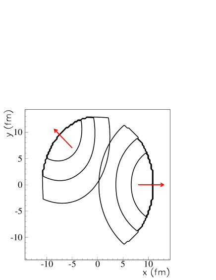
Figure 18: (Color online) Emission probability contours, plotted on a linear scale, indicate emission zones for pions with $p_{T}=0.3$ GeV/c at $\phi_{p}=0^{\circ}$ and $\phi_{p}=135^{\circ}$ (indicated by arrows), from a blast-wave source with “non-round” default parameters listed in Table 1.

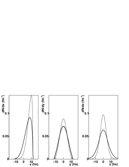
Figure 19: Distribution of the pion spatial distribution in the direction x (left), y (middle) and z (right). Plain line: pion momentum $p_{x}=$ 0.25 GeV/c and $p_{y}=$ 0. Dash line: pion momentum $p_{x}=$ 0.5 GeV/c and $p_{y}=$ 0. Round source parameters of Table 1 were used, with the exception of $a_{s}$ that was set to 0.01.

While the blast-wave parameterization provides direct access to the homogeneity region, the radii extracted from two-pion interferometry are compared to second order moments calculated as shown in equation III.3. Such comparison is strictly correct only if the homogeneity regions are Gaussian distributions. Figure 19 shows an example of spatial distributions along the 3 Cartesian directions for pions with two different momenta, $\overrightarrow{p}$= (0.25 GeV/c, 0, 0) and $\overrightarrow{p}$= (0.5 GeV/c, 0, 0); in this case, the $x-$, $y-$ and $z-$ directions correspond to “out,” “side” and “long,” respectively The $z$ distribution is nearly Gaussian; the difference between the $\sigma$ extracted from a Gaussian fit and the second order moment is on the order of a few percent. On the other hand, the $x$ and $y$ distributions are clearly not Gaussian. To estimate the level of distortion introduced by the non-Gaussian shape, we compare the second order moments with the Gaussian $\sigma$ extracted by fitting the peak of the spatial distributons. Indeed, it has been shown in  HardtkeVoloshin that calculating correlation function from models and fitting them as experimental data yields radii that are close to the Gaussian $\sigma$ extracted by fitting the peak of the spatial distributons. In both the $x-$ and $y-$ directions, we find that the Gaussian $\sigma$ are systematically larger than the second order moments by up to 20% (depending on the fit range) for pions at $p_{T}=$ 0.25 GeV/c. This discrepancy diminishes when increasing the transverse momentum or the particle mass. E.g. it is on the order of 10% for pions at $p_{T}=$ 0.5 GeV/c or for kaons at $p_{T}=$ 0.25 GeV/c. Thus, comparing second order moments with the radii extracted from two-pion correlation functions may involve significant systematic errors at low transverse mass. This issue may be overcome by calculating correlation functions from the Blast Wave space-time distributions or by relying on imaging method to extract space-time distributions from the data HBTImaging . Applying these methods is beyond the scope of this paper and we will thus carry on keeping in mind that systematic errors are associated with comparing HBT radii with second order moment at low transverse momentum.

On the other hand, resonance decay may introduce a core-halo pattern in the distribution of particle space-time emission points CoreHalo . Indeed, some resonances decay sufficiently far away from the bulk of the system that their decay products emerge beyond the main homogeneity region. Such particles form a halo around the core of the source. However, to affect the extracted radii, the resonance lifetime needs to be short enough for the correlation to take place at a relative momentum accesible to the experiment. This lifetime is typically between 10 and 100 fm. The effect of resonance feed-down on radii measured by two-pion interferometry has been studied within a early version of the blast wave parameterization HeinzResonance . It was found that the $\omega$ meson leads to a halo effect, its $c\tau$ being 23.4 fm. The other resonances have lifetimes that are either too short (e.g. $\rho$, $\Delta$) or too long (e.g. $\eta$, $K^{0}_{s}$). At RHIC energy, thermal models Magestro show that about 10% of the pions come from $\omega$, which means that this effect should be rather small. The effect of the very long-lived ($c\tau>100$ fm) resonances is usually assumed to reduce the so-called $\lambda$ parameter CoreHalo2 , which we do not discuss here.

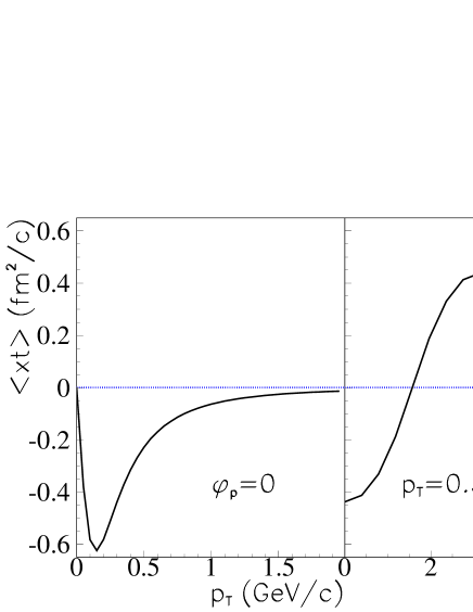
Figure 20: (Color online) Space-time correlation $\langle\tilde{x}\tilde{t}\rangle$ as a function of $p_{T}$ for $\phi_{p}=0$ (left panel), and as a function of $\phi_{p}$ for $p_{T}=0.3$ GeV/c. “Non-round” source parameters of Table 1 were used.

Also important are temporal effects, including space-time correlations. The average $x-t$ correlation, quantified by $\langle\tilde{x}\tilde{t}\rangle$, for the same anisotropic source, is plotted in Figure 20, as a function of $p_{T}$ and $\phi_{p}$. In the left panel, $\phi_{p}=0^{\circ}$, and thus $x$ is the “out” direction. We first note that the correlation is negative, tending to increase $R^{2}_{o}$ for finite $\beta_{\perp}$ (see Equation III.3); large and negative “out”-$t$ correlations at freezeout in some hydrodynamical models RG96 have been a significant component of predicted large $R^{2}_{o}/R^{2}_{s}$ ratios. As required by symmetry HHLW02 , $\langle\tilde{x}\tilde{t}\rangle$ displays an odd-order cosine dependence on $\phi_{p}$; clearly the first-order component dominates here, as shown in the right panel of Figure 20. This $\cos(\phi_{p})$-dependence is driven mostly by the $\cos(\phi_{s})$ dependence of the $x$ coordinate, coupled with the radial flow which tends to make $\phi_{s}\approx\phi_{p}$ (c.f. Figure 18). However, we also note from the figure that the scale of these correlations is $\lesssim 1$ fm²/c, which, as we shall see, is much smaller than the typical scale of $R^{2}_{o}$; hence, space-time correlations do not dominate in the blast-wave.

More important are the correlation coefficients $\langle\tilde{x}\tilde{y}\rangle$, $\langle\tilde{x}^{2}\rangle$ and $\langle\tilde{y}^{2}\rangle$, and their $p$-dependence. $\langle\tilde{x}\tilde{y}\rangle$ quantifies the transverse “tilt” of the emission zone with respect to the reaction plane. As required by symmetry HHLW02 , this tilt vanishes at $\phi_{p}=0$, while, in the present case with $R_{y}>R_{x}$, it is positive for $\phi_{p}=135^{\circ}$ (see Figure 18). That $\langle\tilde{x}^{2}\rangle$ and $\langle\tilde{y}^{2}\rangle$ also depend on $\phi_{p}$ is likewise clear from Figure 18. As we shall see, the $\phi_{p}$-dependence of $\langle\tilde{x}\tilde{y}\rangle$, $\langle\tilde{x}^{2}\rangle$, and $\langle\tilde{y}^{2}\rangle$, combined with the explicit $\phi_{p}$-dependences in Equation III.3, drive the oscillations in HBT radii which we will study.

At this point, it is worthwhile to mention that the emission zone (“homogeneity region”) and the correlation coefficients ($\langle\tilde{x}^{2}\rangle$, $\langle\tilde{y}^{2}\rangle$, $\langle\tilde{x}\tilde{y}\rangle$, $\langle\tilde{x}\tilde{t}\rangle$, $\langle\tilde{y}\tilde{t}\rangle$) will vary with $\phi_{p}$ also for an azimuthally isotropic source ($R_{x}=R_{y}$, $\rho_{2}=0$). However, of course, the measured HBT radii will be $\phi_{p}$-independent. This arises due to cancellation and combination of terms in Equations III.3. For $R^{2}_{s}$, the first term becomes $\phi_{p}$-independent, and the second and third terms combined are $\phi_{p}$-independent ($\left(\langle\tilde{x}^{2}\rangle-\langle\tilde{y}^{2}\rangle\right)\propto\cos(2\phi_{p})$ and $\langle\tilde{x}\tilde{y}\rangle\propto\sin(2\phi_{p})$). For $R^{2}_{o}$, the story is the same for the first three terms, while the fourth term becomes $\phi_{p}$-independent as $\langle\tilde{x}\tilde{t}\rangle\propto\cos(\phi_{p})$ and $\langle\tilde{y}\tilde{t}\rangle\propto\sin(\phi_{p})$. Meanwhile, for $R^{2}_{os}$, the first and second terms cancel each other, as do the two components of the third term; hence $R^{2}_{os}=0$ for azimuthally-symmetric sources. We mention these points here because several of the exact cancellations and combinations which hold for an isotropic source, continue to hold approximately even when the geometry or flow field is anisotropic.

We turn now to a detailed study of the observable HBT radius parameters, and the effects of varying blast-wave parameters. For a boost-invariant system, the symmetry-allowed $\phi_{p}$ oscillations of the (squared) HBT radii are HHLW02

$$R_{s}^{2}(p_{T},\phi_{p}) = R_{s,0}^{2}(p_{T})+{\textstyle 2\sum_{n=2,4,6,\dots}}R_{s,n}^{2}(p_{T})\cos(n\phi_{p}),$$

$$R_{o}^{2}(p_{T},\phi_{p}) = R_{o,0}^{2}(p_{T})+{\textstyle 2\sum_{n=2,4,6,\dots}}R_{o,n}^{2}(p_{T})\cos(n\phi_{p}),$$

$$R_{os}^{2}(p_{T},\phi_{p}) = {\textstyle 2\sum_{n=2,4,6,\dots}}R_{os,n}^{2}(p_{T})\sin(n\phi_{p}),$$ (28)

$$R_{l}^{2}(p_{T},\phi_{p}) = R_{l,0}^{2}(p_{T})+{\textstyle 2\sum_{n=2,4,6,\dots}}R_{l,n}^{2}(p_{T})\cos(n\phi_{p}),$$

where the HBT radii Fourier coefficients $R^{2}_{\mu,n}$ ($\mu=o,s,os,l$ and $n=0,2,4,\dots$) are $\phi_{p}$-independent.

Figure 21 shows the $p_{T}$ and $\phi_{p}$ dependence of HBT radii calculated for a blast-wave source with a slightly anisotropic flow field and shape. In addition to an overall decrease in the average value of the HBT radii with increasing $p_{T}$, we observe significant oscillations in the transverse radii $R^{2}_{o}$, $R^{2}_{s}$, $R^{2}_{os}$, and smaller oscillations in $R^{2}_{l}$.

Figure 21: Squared HBT radius parameters calculated with Equations III.3 and III.3 from a blast-wave source with the “non-round” default parameters of Table 1. Squared radii for various cuts in $p_{T}$ are plotted versus $\phi_{p}$, the emission angle which respect to the event plane.

The Fourier coefficients may be calculated as

$$R^{2}_{\mu,n}(p_{T})=\begin{cases}\langle R^{2}_{\mu}(p_{T},\phi_{p})\cos(n\phi_{p})\rangle&(\mu=o,s,l)\\ \langle R^{2}_{\mu}(p_{T},\phi_{p})\sin(n\phi_{p})\rangle&(\mu=os)\end{cases}.$$ (29)

In the present model, we find that oscillation amplitudes above 2^nd order are very small in all cases considered ($|R^{2}_{\mu,4}/R^{2}_{\mu,2}|\lesssim 0.01$). Therefore, the $\phi_{p}$-dependence of the HBT radii at a given $p_{T}$ is essentially encapsulated in seven numbers: the 0^th- and 2^nd-order Fourier coefficients of $R^{2}_{o}$, $R^{2}_{s}$, and $R^{2}_{l}$, and the 2^nd-order Fourier coefficient of $R^{2}_{os}$. We henceforth explore the evolution of the $p_{T}$-dependence of these seven numbers, as model parameters are varied.

Figure 22: Fourier coefficients of the $\phi_{p}$-dependence of the squared HBT radii, as calculated by Equation 29. $0^{\rm th}$- and $2^{\rm nd}$-order Fourier coefficients are plotted in the left and right panels, respectively. The transverse shape of the source (i.e. $R_{y}/R_{x}$) was varied, while $R^{2}_{y}+R^{2}_{x}$ was held fixed. “Round” source values from Table 1 are used for the other parameters.

Figure 22 shows the Fourier coefficients for $n=0,2$, corresponding to a blast-wave source with $T=0.1$ GeV, an isotropic flow field ($\rho_{0}=0.9$, $\rho_{2}=0$), a box profile ($a_{s}=0$), and time parameters $\tau_{0}=9$ fm/c, $\Delta\tau=2$ fm/c. Here, the average transverse size of the source ($R^{2}_{x}+R^{2}_{y}$) was held fixed, while the shape ($R_{y}/R_{x}$) was varied.

The $0^{\rm th}$-order Fourier coefficients (corresponding to the radii $R_{o}$, $R_{s}$, and $R_{l}$ usually measured by experimentalists) are sensitive only to the average scale, not the shape, of the source. The average values of the transverse radii $R^{2}_{o,{0}}$ and $R^{2}_{s,{0}}$ fall with increasing $p_{T}$ due to radial flow WH99 ; WSH96 (c.f. Figure 31). At intermediate values of $p_{T}$, $R^{2}_{o,{0}}>R^{2}_{s,{0}}$ due to finite timescale effects (cf Figures 29 and 30), but at high $p_{T}$, $R^{2}_{o,{0}}<R^{2}_{s,{0}}$ (i.e. $R_{o}/R_{s}<1$), in qualitative agreement with experimental data PhenixHBT ; STARHBT . The boost-invariant longitudinal flow produces the strong decrease of $R^{2}_{l,{0}}$ with $p_{T}$ WH99 ; MS88 ; AS95 ; HB95 ; WSH96 .

Richer detail is seen in the oscillations of the HBT radii, quantified by Fourier coefficients $R^{2}_{\mu,{2}}$ in the right-hand panels of Figure 22. Here, the elliptical shape of the source is explicitly clear. The signs of the $2^{\rm nd}$-order Fourier coefficients of the transverse radii directly reflect the out-of-plane-extended source geometry when $R_{y}>R_{x}$. $R^{2}_{os,{2}}$ has a similar geometric interpretation, in terms of the $\phi_{p}$-evolution of the “tilt” of the homogeneity region HK02 . The relatively small oscillations in $R^{2}_{l}$ arise not directly from geometry, but instead from transverse flow gradients, which slightly reduce $R^{2}_{l}$ WSH96 . In the present example, the transverse flow increases linearly from 0 (at the center) to $\rho_{0}=0.9$ (at the edge of the source), independent of boost angle $\phi_{b}$. However, when $R_{y}>R_{x}$, the flow gradient is larger for source elements boosted in-plane, leading to slightly greater reduction of $R^{2}_{l}$ when $\phi_{p}=0$; hence $R^{2}_{l,{2}}<0$.

Finally, we recall that the flow field is isotropic ($\rho_{2}=0$) and so all $\phi_{p}$-dependence arises from geometry here. Thus, if the values of $R_{y}$ and $R_{x}$ are interchanged (corresponding to in-plane-extended sources), $R^{2}_{\mu,{0}}$ would remain unchanged, and $R^{2}_{\mu,{2}}$ would simply change in sign in Figure 22.

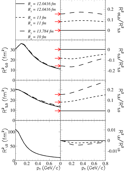
Figure 23: (Color online) Identical data as in Figure 22, except the right panels show ratios of $2^{\rm nd}$-order and $0^{\rm th}$ order Fourier coefficients of the $\phi_{p}$-dependence of the squared HBT radii. Arrows indicate values calculated from Equation 32; see text for details.

As discussed above, transverse flow-induced space-momentum correlations tend to decrease homogeneity lengths as $p_{T}$ increases. When combined with other effects (e.g. temporal effects), non-trivial $p_{T}$ dependences of the HBT radii result. The $p_{T}$-dependences of the $\phi_{p}$-averaged values $R^{2}_{\mu,{0}}$ have been discussed extensively WH99 ; WSH96 . Meanwhile, the $p_{T}$-dependences of the oscillation amplitudes ($R^{2}_{\mu,{2}}$) shown in the right panels of Figure 22 have not been explored previously and may be non-trivial in principle.

It was suggested peter_dan_private that the $p_{T}$-dependence of $|R^{2}_{\mu,{2}}|$ might be driven largely by the same effects which generate the $p_{T}$-dependence of $R^{2}_{\mu,{0}}$, and hence the most efficient and direct way to study the source is to plot $R^{2}_{\mu,{0}}$, which encode scale information, and then the ratio of $2^{\rm nd}$- to $0^{\rm th}$-order Fourier coefficients, which would encode geometric and dynamic anisotropy. This is an excellent suggestion, though consideration must be given to the appropriate scaling. First, we consider the transverse radii $R^{2}_{o}$, $R^{2}_{s}$ and $R^{2}_{os}$. The radii $R^{2}_{o}$ and $R^{2}_{os}$ encode both transverse geometry and temporal information. As discussed above, space-time (e.g. $x-t$) correlations are small in magnitude, and furthermore affect the HBT radii in combinations which tend to cancel any $\phi_{p}$-dependence. Therefore, we expect $R^{2}_{o,{0}}$, $R^{2}_{s,{0}}$, $R^{2}_{s,{2}}$, $R^{2}_{o,{2}}$ and $R^{2}_{os,{2}}$ to contain geometric contributions, while temporal contributions are significant only for $R^{2}_{o,{0}}$. In this case, the appropriate ratios to study are $R^{2}_{o,{2}}/R^{2}_{s,{0}}$, $R^{2}_{s,{2}}/R^{2}_{s,{0}}$ and $R^{2}_{os,{2}}/R^{2}_{s,{0}}$. Indeed, we find numerically that these are the ratios least affected by the overall scale of the homogeneity region, which varies both with $p_{T}$ and with model parameter. The oscillation strength $R^{2}_{l,{2}}$ of the longitudinal radius, on the other hand, is entirely due to implicit $\phi_{p}$ dependences driven by space-momentum correlations; these same correlations affect $R^{2}_{l,{0}}$. Hence, the appropriate ratio to study in this case is $R^{2}_{l,{2}}/R^{2}_{l,{0}}$.

In Figure 23 we show these ratios for the same sources as were plotted in Figure 22. The $p_{T}$-dependence of the ratios is significantly less than that of the oscillation strengths $R^{2}_{\mu,{2}}$, as anticipated, due to the fact that the latter is driven largely by space-momentum correlations reducing the spatial scale of the homogeneity region.

Going further, we may recall that in the special case of vanishing space-momentum correlations ($\rho=0$ or $T=\infty$), the transvserse radii oscillate with identical strengths ($R^{2}_{os,{2}}=R^{2}_{s,{2}}=-R^{2}_{o,{2}}$), and the in-plane and out-of-plane extents of the source may be directly extracted W98 ; LHW00 ; HHLW02 ; E895HBTwrtRP , as the “whole source” is viewed from every angle. In that special case, independent of $p_{T}$

$$R^{2}_{s,{0}}=\frac{1}{2}\left(\langle\tilde{y}^{2}\rangle+\langle\tilde{x}^{2}\rangle\right)=\frac{1}{8}\cdot(R_{y}^{2}+R_{x}^{2})$$ (30)

$$R^{2}_{os,{2}}=R^{2}_{s,{2}}=-R^{2}_{o,{2}} = \frac{1}{4}\left(\langle\tilde{y}^{2}\rangle-\langle\tilde{x}^{2}\rangle\right)$$ (31)

$$= \frac{1}{16}\left(R_{y}^{2}-R_{x}^{2}\right)$$

so that

$$\frac{R^{2}_{os,{2}}}{R^{2}_{s,{0}}}=\frac{R^{2}_{s,{2}}}{R^{2}_{s,{0}}}=-\frac{R^{2}_{o,{2}}}{R^{2}_{s,{0}}}=\frac{1}{2}\cdot\frac{R_{y}^{2}-R_{x}^{2}}{R_{y}^{2}+R_{x}^{2}}\equiv\frac{\epsilon}{2}$$ (32)

In the presence of flow, however, HBT radii measured at momentum $\vec{p}$ reflect homogeneity lengths which in principle may vary nontrivially both with $p_{T}$ and $\phi_{p}$. While we find that non-vanishing flow violates the $p_{T}$-independence of $R^{2}_{s,{0}}$, $R^{2}_{o,{2}}$, $R^{2}_{s,{2}}$ and $R^{2}_{os,{2}}$ (and thus Equations 30 and 31), Equation 32 remains remarkably robust. As seen in the next several Figures, the ratios $R^{2}_{o,{2}}/R^{2}_{s,{0}}$, $R^{2}_{s,{2}}/R^{2}_{s,{0}}$ and $R^{2}_{os,{2}}/R^{2}_{s,{0}}$, largely independent of $p_{T}$, provide an estimate of the source ellipticity $\epsilon$. Arrows to the left of the panels for $R^{2}_{o,{2}}/R^{2}_{s,{0}}$, $R^{2}_{s,{2}}/R^{2}_{s,{0}}$ and $R^{2}_{os,{2}}/R^{2}_{s,{0}}$ in Figures 23-34 indicate $\epsilon/2$ for the sources used.

Now that we have established the quantities to be examined in this Section, we briefly check the importance of using quantum, rather than classical, statistics in the source function of Equation II.3. Setting the parameter values to correspond to the “non-round” source of Table 1, we plot in Figure 24 the Fourier coefficients corresponding to different values of $N$, where the summation in Equation II.3 (and Equations II.3 and 18) is over $n=1\ldots N$. Once again, we find a small difference between the curves for $N=1$ and $N>1$, while inclusion of higher terms in the summation have essentially no effect. Blast-wave calculations in this Section correspond to $N=2$.

Figure 24: (Color online) Fourier coefficients of the $\phi_{p}$-dependence of the squared HBT radii, as calculated by Equation 29 using several values of $N$, the maximum value of $n$ taken in the summation of Equation II.3. Values of the blast-wave parameters are for a “non-round” source, as listed in Table 1. Arrows indicate values calculated from Equation 32. See text for details.

Recently, Heinz and Kolb, in a hydrodynamic model, calculated HBT radii as a function of $\phi_{p}$ for non-central collisions HK02 . They used two different Equations of State and initial conditions: one (“RHIC”) is appropriate for soft physics at RHIC energies, and has successfully reproduced momentum-space observables HK01 ; the other (“IPES”) assumes extremely high initial energy densities, perhaps appropriate for collisions at LHC energies.

It is worthwhile to point out that even the “RHIC” hydrodynamic calculations fail to reproduce azimuthally-integrated HBT data HK01 ; here, however, we simply investigate the connection between the freeze-out geometry and oscillations of the HBT radii. Both calculations result in a freeze-out configuration, integrated over $p_{T}$, which is rather sharp-edged in transverse coordinate-space; thus, we may extract surface radii $R_{x}$ and $R_{y}$ to calculate $\epsilon$.

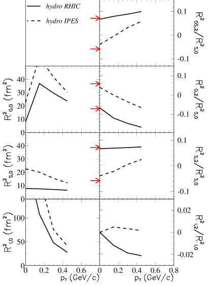
Figure 25: (Color online) Fourier coefficients of the $\phi_{p}$-dependence of the squared HBT radii, as calculated by Equation 29. The data are not from blast-wave calculations, but from hydrodynamic calculations of Heinz and Kolb HK02 , for two different equations of state and initial conditions. Arrows indicate values calculated from Equation 32 and extracted values of freezeout edge radii; see text for details.

Figure 25 shows the same quantities as plotted in Figure 23, but extracted from these hydrodynamic calculations. The “RHIC” source, which is geometrically extended out-of-plane ($R_{y}>R_{x}$, resulting in a positive $\epsilon$) generates oscillations in the transverse radii with the same phase as out-of-plane sources in blast-wave calculations. For this source, the connection between $\epsilon$ and the radius oscillations (Equation 32) is most robust for $R^{2}_{s,{2}}$ and least well-satisfied for $R^{2}_{o,{2}}$, an effect not observed in the blast-wave. However, our blast-wave parameterization does not include explicit $\phi_{p}$ dependence of the temporal scale, which would affect $R^{2}_{o,{2}}$, and, to a lesser degree, $R^{2}_{os,{2}}$. Instead of attempting a more sophisticated parameterization, we simply note this fact, and would recommend that an experimental estimation of the source deformation $\epsilon$ is probably best extracted from $R^{2}_{s,{2}}/R^{2}_{s,{0}}$, which should be unaffected by azimuthal structure of the temporal scale. From the study (below) of parameter variations in the blast-wave, the approximation $\epsilon\approx 2R^{2}_{s,{2}}/R^{2}_{s,{0}}$ is good to $\sim$30%, for RHIC-type sources.

Figure 25 also shows results from the “IPES” hydrodynamic calculation. Here, the freeze-out shape is extended in-plane HK02 , but dynamical effects are so strong in this extreme case, that even the sign of the transverse radius oscillations changes with $p_{T}$. The relationships in Equation 32 work only at low $p_{T}$, and even there only very approximately. According to this model, then, geometrical considerations dominate the HBT radius oscillations, while dynamical effects begin to dominate at much higher energies.

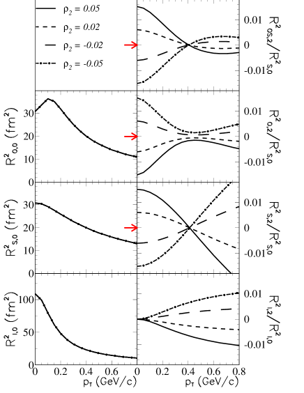
Figure 26: (Color online) Fourier coefficients of the $\phi_{p}$-dependence of the squared HBT radii, as calculated by Equation 29. The anisotropy of the flow field ($\rho_{2}$) is varied. Values of the other parameters are for a “round” source, as listed in Table 1. Arrows indicate values calculated from Equation 32; see text for details.

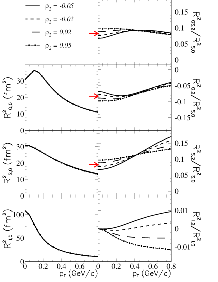
Figure 27: (Color online) Fourier coefficients of the $\phi_{p}$-dependence of the squared HBT radii, as calculated by Equation 29. The anisotropy of the flow field ($\rho_{2}$) is varied. Values of the other parameters are for a “non-round” source, as listed in Table 1. Arrows indicate values calculated from Equation 32; see text for details.

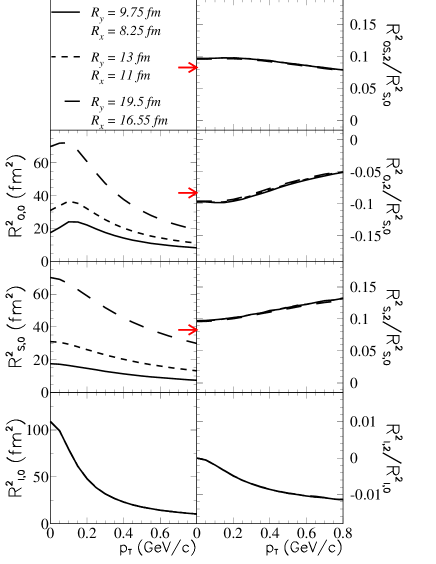
Figure 28: (Color online) Fourier coefficients of the $\phi_{p}$-dependence of the squared HBT radii, as calculated by Equation 29. The overall transverse scale ($\sqrt{R_{y}^{2}+R_{x}^{2}}$) is varied, while keeping $R_{y}/R_{x}=13/11$. Values of the other parameters are for a “non-round” source, as listed in Table 1. Arrows indicate values calculated from Equation 32; see text for details.

In Figure 26, the source geometry is azimuthally isotropic ($R_{x}=R_{y}=12.042$ fm), while the flow field is varied from having a stronger boost in-plane ($\rho_{2}>0$) to a stronger boost out-of-plane ($\rho_{2}<0$). We notice again that the average HBT radius values $R^{2}_{\mu,{0}}$ are unaffected by the anisotropy. The oscillations ($R^{2}_{\mu,{2}}$) are driven by flow gradients. Naively, one would expect that all HBT radii $R_{o}$, $R_{s}$, $R_{l}$ would be smaller when the emission angle $\phi_{p}$ is in the direction of the strongest boost. For $\rho_{2}=0.05$, for example, the radii would be smaller at $\phi_{p}=0$, the direction of stronger transverse boost; this would correspond to $R^{2}_{\mu,{2}}<0$ ($\mu=o,s,l$). For $\mu=o$ and $\mu=l$, this is indeed observed, at all $p_{T}$. $R^{2}_{s,{2}}$, however, changes sign from positive at low $p_{T}$, to negative at high $p_{T}$. This behaviour at low $p_{T}$ is due to an effect similar to that which led to negative proton $v_{2}$ at low $p_{T}$, even when $\rho_{2}>0$. (See discussion surrounding Figure 12.) In the present case, the particles with $p_{T}\approx 0$ are more likely to be emitted by source elements positioned along the $y$-axis, due to the strong in-plane boost for source elements with large spatial coordinate $x$. The homogeneity region for $p_{T}=0$ particles is independent of $\phi_{p}$, and has larger extent out-of-plane than in-plane. Thus we find the counter-intuitive result that $R^{2}_{s}(\phi_{p}=0)>R^{2}_{s}(\phi_{p}=\frac{\pi}{2})\rightarrow R^{2}_{s,{2}}>0$ at $p_{T}\approx 0$. We note that a similar argument holds for $R^{2}_{o}$, except that it leads to the conclusion that $R^{2}_{o,{2}}<0$ at $p_{T}\approx 0$, and so goes in the same direction as flow-gradient effects. It is only for $R^{2}_{s}$ that the two effects compete.

Finally, comparing the scales on the right-hand panels of Figures 23 and 26, it is clear that, while the $2^{\rm nd}$-order coefficients are driven by both anisotropic geometry and flow field, a variation in geometry ($R_{y}/R_{x}$) has a stronger effect on $R^{2}_{\mu,{2}}$ than a variation in $\rho_{2}$, when these parameters are varied by amounts which would generate a similar effect on elliptic flow $v_{2}$ (cf Figures 14 and 16). Thus, measurement of both $v_{2}$ and HBT radius oscillations would allow independent determination of both anisotropic flow strength $\rho_{2}$ and shape $R_{y}/R_{x}$.

In Figure 27, we consider anisotropy simultaneously in both the source geometry and the flow field. The source is extended out-of-plane ($R_{y}=13$ fm and $R_{x}=11$ fm), and the flow anisotropy ($\rho_{2}$) varied. The $0^{\rm th}$-order coefficients remain unaffected by the anisotropies, while the $R^{2}_{\mu,{2}}$ reflect essentially the cumulative effects of the geometric anisotropy (shown in Figure 23) and the flow field anisotropy (shown in Figure 26), with no strong non-linear coupling between them. Thus, while in principle anisotropic flow effects may mask or dominate geometric anisotropy HK01 , flow field anisotropies represent small perturbations on the dominant geometric effects in the blast-wave, using “realistic” (cf Section 4) parameters.

In Figure 28 we show the effect of increasing the transverse size of the source ($\sqrt{R_{y}^{2}+R_{x}^{2}}$) while keeping the shape ($R_{y}/R_{x}$) and other source parameters fixed. As expected, the purely-spatial transverse radius $R_{s}^{2}$ (average and oscillation amplitude) increases proportionally with $R_{y}^{2}+R_{x}^{2}$. The squared “outward” radius parameter, $R_{o}^{2}$, contains both spatial components (which increase with $R_{y}^{2}+R_{x}^{2}$) and temporal components (which do not). Thus, its average value, $R^{2}_{o,{0}}$, increases almost proportional to $R_{y}^{2}+R_{x}^{2}$ at low $p_{T}$ ($\beta_{\perp}\sim 0$) and less so at higher $p_{T}$. Due to the near-cancellation of $\phi_{p}$-dependence of temporal terms, the increase in oscillation amplitudes $R^{2}_{os,{2}}$ and $R^{2}_{os,{2}}$ is driven mainly by the spatial terms, so that $R^{2}_{o,{2}}/R^{2}_{s,{0}}$ and $R^{2}_{os,{2}}/R^{2}_{s,{0}}$ display almost no sensitivity to $R_{y}^{2}+R_{x}^{2}$ at any $p_{T}$. The longitudinal radius $R_{l}^{2}$ is unaffected by variation in the transverse scale.

Figure 29: (Color online) Fourier coefficients of the $\phi_{p}$-dependence of the squared HBT radii, as calculated by Equation 29. The evolution duration $\tau_{0}$ is varied. Values of the other parameters are for a “non-round” source, as listed in Table 1. Arrows indicate values calculated from Equation 32; see text for details.

In Figures 29 and 30, we vary the timescale parameters $\tau_{0}$ and $\Delta\tau$, respectively. All dependence of $R^{2}_{\mu,{n}}$ on these parameters come directly through the dependence of $\langle\tilde{x}_{\mu}\tilde{x}_{\nu}\rangle$, which are listed explicitly in Equations III.3. After an inspection of those equations, it is unsurprising that the effects of varying these parameters are similar. The space-time correlation coefficients which depend on the timescale parameters are $\langle\tilde{x}\tilde{t}\rangle$, $\langle\tilde{y}\tilde{t}\rangle$, $\langle\tilde{t}^{2}\rangle$, and $\langle\tilde{z}^{2}\rangle$. According to Equation III.3, then, $R^{2}_{s,{0}}$ and $R^{2}_{s,{2}}$ are unaffected by variations in $\tau_{0}$ and $\Delta\tau$. $R^{2}_{l}=\langle\tilde{t}^{2}\rangle$ is directly proportional to $\left(3\Delta\tau^{2}+\tau_{0}^{2}\right)$, so $R^{2}_{l,{0}}$ and $R^{2}_{l,{2}}$ both scale with that quantity. Turning to the HBT radii with both spatial and temporal contributions, we again find that the $\phi_{p}$-dependence of the temporal terms is negligible, so that $R^{2}_{o,{2}}/R^{2}_{s,{0}}$ and $R^{2}_{os,{2}}/R^{2}_{s,{0}}$ are independent of the timescales, while $R^{2}_{o,{0}}$ displays the well-known WH99 sensitivity to timescale.

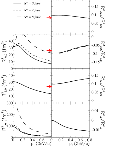
Figure 30: (Color online) Fourier coefficients of the $\phi_{p}$-dependence of the squared HBT radii, as calculated by Equation 29. The evolution duration $\Delta\tau$ is varied. Values of the other parameters are for a “non-round” source, as listed in Table 1. Arrows indicate values calculated from Equation 32; see text for details.

Thus, we find that, in the blast-wave parameterization, essentially all sensitivity to timescales comes through the $\phi_{p}$-independent quantities $R^{2}_{o,{0}}$ and $R^{2}_{l,{0}}$. However, it is important to point out that an experimental estimate of the freeze-out geometric anisotropy, defined in Equation 32, from measurements of the $R^{2}_{\mu,{n}}$ would place an additional constraint on the evolution timescale $\tau_{0}$. In particular, the large initial-state anisotropy in coordinate space ($R_{y}>R_{x}$) in a non-central collision will be reduced due to stronger flow in-plane than out-of-plane ($\rho_{2}>0$ in the present parameterization). If the source lives for a long time (large $\tau_{0}$), the system may become round ($R_{y}=R_{x}$) or even in-plane extended ($R_{y}<R_{x}$) TLS01 . A quantitative constraint on $\tau_{0}$ from the relationship of the initial to freeze-out anisotropies, however, must be made in the context of a realistic dynamical model and is beyond the scope of the blast-wave parameterization.

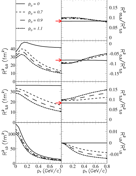
Figure 31: (Color online) Fourier coefficients of the $\phi_{p}$-dependence of the squared HBT radii, as calculated by Equation 29. The average radial flow magnitude $\rho_{0}$ is varied. Values of the other parameters are for a “non-round” source, as listed in Table 1. Arrows indicate values calculated from Equation 32; see text for details.

In Figure 31, the effect of variations in the $\phi$-averaged (“radial”) flow on the HBT radius parameters is shown. As is well-known WH99 , stronger flow reduces the homogeneity lengths, and, indeed, almost all of the $|R^{2}_{\mu,{n}}|$ fall with increasing $\rho_{0}$. The one interesting exception is $R^{2}_{l,{2}}$; while the average scale of the longitudinal radius ($R^{2}_{l,{0}}$) decreases as the flow is increased, its $\phi_{p}$-dependence ($|R^{2}_{l,{2}}|$) increases (and so, then, does $|R^{2}_{l,{2}}/R^{2}_{l,{0}}|$). This is because there is no explicit $\phi_{p}$ dependence in $R^{2}_{l}=\langle\tilde{z}^{2}\rangle$; any $\phi_{p}$ dependence is implicit, and thus is generated by space-momentum correlations W98 , which, in this model, arise solely from flow. In the no-flow limit for a boost-invariant source, $\langle\tilde{t}^{2}\rangle$, $\langle\tilde{x}^{2}\rangle$, $\langle\tilde{y}^{2}\rangle$, and $\langle\tilde{z}^{2}\rangle$ are all $\phi_{p}$-independent constants W98 ; LHW00 ; HHLW02 .

Indeed, it is for a similar reason that $R^{2}_{l,{2}}$ vanishes for $p_{T}=0$, independent of model parameter in Figures 23-32. At $p_{T}=0$, symmetry demands that none of the spatial correlation coefficients $\langle\tilde{x}_{\mu}\tilde{x}_{\nu}\rangle$ may depend on $\phi_{p}$. Hence, only HBT radii with explicit $\phi_{p}$-dependence may exhibit an oscillation in that limit.

Finally, we note in Figure 31 that the oscillation strengths $|R^{2}_{o,{2}}|$ and $|R^{2}_{s,{2}}|$ are somewhat less diminished (at low $p_{T}$) by increasing radial flow, than is $R^{2}_{s,{0}}$, which measures the overall spatial scale of the homogeneity region. Here, we offer no simple insights on the interplay between the increasing deformation of the homogeneity region, and its decreasing scale, but simply note that the dependence of the scaled oscillation strengths on $\rho_{0}$ is rather small, especially at low $p_{T}$, even for the unrealistic case of no average transverse flow ($\rho_{0}=0$).

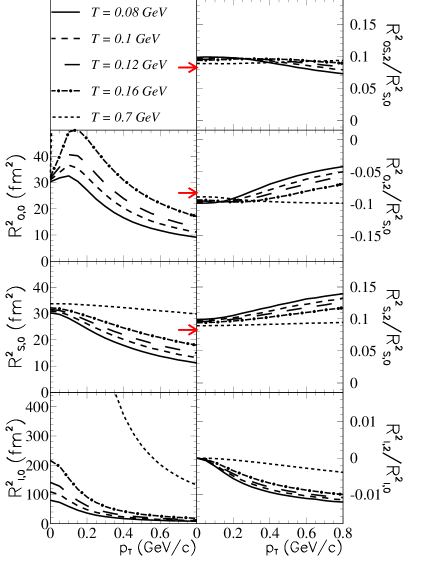
Figure 32: (Color online) Fourier coefficients of the $\phi_{p}$-dependence of the squared HBT radii, as calculated by Equation 29. For $T=0.7$ GeV/c, $R^{2}_{o,{0}}$ and $R^{2}_{l,{0}}$ curves partially exceed the displayed scale. Values of the other parameters are for a “non-round” source, as listed in Table 1. Arrows indicate values calculated from Equation 32; see text for details.

Figure 32 explores the effect on HBT radii of varying the temperature parameter $T$. Increasing $T$ increases “thermal smearing”, reducing the flow-induced space-momentum correlations. It is well known that this leads to increased homogeneity lengths and HBT radii SSH93 , as reflected in the left panels of the Figure. In the present model, we find a small residual dependence of $R^{2}_{\mu,{2}}$ on $T$ beyond the scaling of $R^{2}_{\mu,{0}}$ (right panels).

In the limit of very high temperature, all space-momentum correlations are eliminated, and all oscillations of HBT radii are again due to the explicit $\phi_{p}$-dependence in Equations III.3. Then, we find that Equations 30-32 hold, independent of $p_{T}$. For the source of Figure 32, according to Equation 32, $|R^{2}_{\mu,{2}}/R^{2}_{s,{0}}|=0.083$. Finally, $R^{2}_{l,{2}}$ decreases with increasing $T$, and must vanish at $T\rightarrow\infty$, when all space-momentum correlations are destroyed.

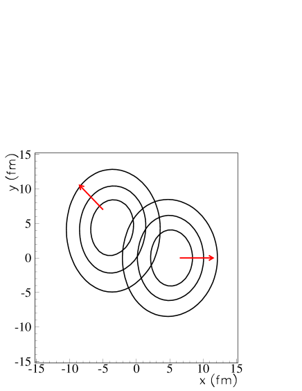
Figure 33: (Color online) Emission probability contours, plotted on a linear scale, indicate emission zones for pions with $p_{T}=0.3$ GeV/c at $\phi_{p}=0^{\circ}$ and $\phi_{p}=135^{\circ}$ (indicated by arrows), from a blast-wave source with $a_{s}=0.3$. Other parameter values correspond to the “non-round” values listed in Table 1.

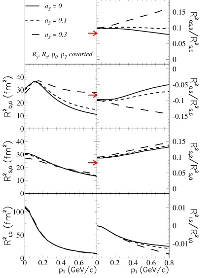
Figure 34: (Color online) Fourier coefficients of the $\phi_{p}$-dependence of the squared HBT radii, as calculated by Equation 29. The parameters $T$, $\tau_{0}$ and $\Delta\tau$ are set to values listed in Table 1, while the parameters $\rho_{0}$, $\rho_{2}$, $R_{y}$ and $R_{x}$ are co-varied with the surface diffuseness $a_{s}$; see text for details.

Finally, we consider the effect of a finite “skin thickness” $a_{s}$. As in the discussions surrounding Figures 7 and 17, it is appropriate to scale the flow parameters according to $F(a_{s})$ given in Equation 20. Moreover, it is clearly appropriate to scale the geometric size parameters $R_{y}$ and $R_{x}$, as the overall scale of the source will increase with $a_{s}$, if these parameters remain fixed. Less clear is the exact scaling which would keep, e.g. $R^{2}_{s,{0}}$, independent of $a_{s}$, especially in the presence of finite flow. For illustrative purposes, we scale $R_{y}$ and $R_{x}$ also by $F(a_{s})$, so that $R_{y}$ = 13.0, 12.21, and 8.84 fm, for $a_{s}$ = 0, 0.1, and 0.3, respectively; $R_{y}/R_{x}=13/11$ in all cases. This scaling keeps $\langle|r|\rangle$, as well as the flow gradient, the same in each case.

Figure 33 shows homogeneity regions projected onto the $x-y$ plane, for a blast-wave source with $a_{s}=0.3$, corresponding to a pseudo-Gaussian geometrical distribution in $\tilde{r}$ (see Figure 1). Comparing Figures 18 and 33, we observe that the lack of a “hard cut-off” in coordinate space in the latter case leads to less reduction in the “out” direction (i.e. along the direction of motion). Thus, the important ratio $R^{2}_{o,{0}}/R^{2}_{s,{0}}$ will be larger at finite $p_{T}$, when $a_{s}=0.3$.

We also note that the shape and size of the homogeneity region itself depends much less on $\phi_{p}$, when $a_{s}=0.3$. The homogeneity region for pions emitted to $\phi_{p}=135^{\circ}$ is essentially a spatially-translated (and unrotated) replica of that for pions emitted to $\phi_{p}=0^{\circ}$. Since HBT correlations are insensitive to a spatial translation of the source, the situation for $a_{s}=0.3$ is rather similar to the situation in which no flow is present. In the no-flow case, the same homogeneity region is measured at all angles, and all oscillations of the HBT radii arise from the explicit $\phi_{p}$ dependence in Equations III.3 W98 ; LHW00 ; for the source in Figure 33, not the same region, but a (virtually) identical one, is being measured at all angles $\phi_{p}$.

This has implications for the oscillations of the transverse radii. Focusing on the homogeneity regions for $\phi_{p}=135^{\circ}$, we observe that while $\langle\tilde{x}\tilde{y}\rangle$ (which quantifies the “tilt” of the homogeneity region relative to the $x$ and $y$ axes) is greater when $a_{s}=0$, $R_{os}^{2}$ (which quantifies the tilt of the homogeneity region relative to the “out” and “side” directions HK02 ) is larger for $a_{s}=0.3$ Therefore, we expect larger values of $R^{2}_{os,{2}}$ for larger $a_{s}$.

Figure 34 shows quantitatively the effects on the HBT radii, when $a_{s}$ is varied. As intended by the scaling of flow and size parameters with $F(a_{s})$, $R^{2}_{s,{0}}$ remains approximately invariant when the parameters are covaried. As discussed above, $R^{2}_{o,{0}}/R^{2}_{s,{0}}$ grows with $a_{s}$ at finite $p_{T}$, as do the magnitudes of the oscillation strengths $|R^{2}_{o,{2}}/R^{2}_{s,{0}}|$, $|R^{2}_{os,{2}}/R^{2}_{s,{0}}|$ and $|R^{2}_{s,{2}}/R^{2}_{s,{0}}|$. The average value of $R^{2}_{l}$ remains roughly constant, while its oscillation amplitude increases slightly with $a_{s}$, due to $x-z$ and $y-z$ correlations.

III.4 Non-identical particle correlations

Final-state interactions between pairs of non-identical particles (e.g. $K-\pi$) are sensitive to the space-time structure (size, shape, emission duration) of the emitting source, analogously to HBT correlations between identical particles. Most importantly, the authors of Ref. PLBNonId ; LedNonId ; PRLNonId show that studying correlations between non-identical particles reveals new information about the average relative space-time separation between the emission of the two particles, in the rest frame of the pair. This unique information may be extremely valuable to determine the interplay between partonic and hadronic effects. For example, the lower hadronic cross-section of kaons compared to pions may cause them to be emitted earlier and closer to the center of the source than pions. However, if most of the system evolution takes place at the parton level, the space-time emission pattern of pions and kaons would be similar. This example is far from unique as the same kind of argument can be made for protons recalling that pion-proton hadronic cross section are very large, or conversely to $\Xi$ and $\Omega$ whose hadronic cross section is expected to be small. Furthermore, in terms of temporal effects, strangeness distillation StrangeDistil ; earlyStrangeDistil or other unique physics may cause some particles to be emitted later than others. Preliminary analyses of the $\pi^{\pm}-K^{\pm}$, $\pi^{\pm}-p^{\pm}$, $K^{\pm}-p^{\pm}$ correlation functions have been reported by the STAR collaboration in Au-Au collisions at $\sqrt{s_{NN}}=$130 GeV and 200 GeV QM03NonId ; PiKPRL . These analyses show that pions, kaons and protons are not emitted at the same average space-time point.

The blast-wave parameterization implicitly assumes that the particle freeze-out conditions (temperature, flow profile, freeze-out time and position) are the same for all particle species. However, as shown earlier, the transverse momentum spectra and elliptic flow or different particle species do not look alike. Indeed, the relative contribution of the random emission (quantified by temperature) and collective expansion depends directly on particle masses. The same phenomena is likely to affect the particle freeze-out space-time emission distribution. In this section, we will show that collective flow effects implicit in the blast-wave parameterization induce a shift between the average freeze-out space-time point of different particle species. We will then study how changing the blast-wave parameters affects these average freeze-out separations.

III.4.1 Non-identical particle and blast-wave formalism

Two particles interact when they are close to each other in phase space in the local pair rest frame. Thus, particle pairs may be correlated when their relative momentum in the pair rest frame is small. For particles with different masses, a small relative momentum in the pair rest frame means that both particles have similar velocities in the laboratory frame and not similar momentum. This point is particularly important to realize when studying correlation involving pions. Due to the low pion mass, the pion velocity is the same as heavier particles (e.g. kaons or protons) when its momentum is much lower than the particle momentum it is associated with. For example, a proton with a momentum of 1 GeV/c has the same velocity as a pion with a momentum of $\approx$0.15 GeV/c.

As described in Ref. NonIdOutSideLong , the spatial separation between particles in the pair rest frame can be projected along three axes, $\langle r^{*}_{out}\rangle$, along the pair transverse momentum, $\langle r^{*}_{side}\rangle$, perpendicular to the pair transverse momentum and $\langle r^{*}_{long}\rangle$, along the beam axis. To study the blast-wave prediction, we focus on the limiting case where the relative momentum between both particles in the pair rest frame is zero, which means that both particles have the same velocity. Thus we calculate the separation between particle 1 and 2 in the pair rest frame $\langle\Delta r^{*}_{out}\rangle$, $\langle\Delta r^{*}_{side}\rangle$ and $\langle\Delta r^{*}_{long}\rangle$, at a given pair transverse velocity $\beta_{T}$, azimuthal angle, $\phi_{p}$, and longitudinal velocity, $\beta_{L}$:

$$\langle\Delta r^{*}_{out}\rangle = \langle r^{*}_{out}(1)\rangle-\langle r^{*}_{out}(2)\rangle$$ (33)

$$\langle\Delta r^{*}_{side}\rangle = \langle r^{*}_{side}(1)\rangle-\langle r^{*}_{side}(2)\rangle$$ (34)

$$\langle\Delta r^{*}_{long}\rangle = \langle r^{*}_{long}(1)\rangle-\langle r^{*}_{long}(2)\rangle$$ (35)

With the particle emission points defined as ($x,y,z,t$):

$$\langle r^{*}_{out}\rangle = \gamma_{T}(\langle x\rangle\cos(\phi_{p})+\langle y\rangle\sin(\phi_{p})-\beta_{T}\langle t\rangle)$$ (36)

$$\langle r^{*}_{side}\rangle = \langle y\rangle\cos(\phi_{p})-\langle x\rangle\sin(\phi_{p})$$ (37)

$$\langle r^{*}_{long}\rangle = \gamma_{L}\langle(z)-\beta_{L}(t)\rangle$$ (38)

Recalling that $\langle\beta_{L}\rangle=\langle z/t\rangle$, $\langle r^{*}_{long}(i)\rangle=0$. Following the notation of Equation 25, the variables $\langle x\rangle$, $\langle y\rangle$ and $\langle t\rangle$ depend on $\beta_{T}$ and on the particle mass (m) as:

$$\langle x\rangle = \overline{\left\{x\right\}_{0,0}}(m,\beta_{T})$$ (39)

$$\langle y\rangle = \overline{\left\{y\right\}_{0,0}}(m,\beta_{T})$$ (40)

$$\langle t\rangle = \frac{\Delta\tau^{2}+\tau_{0}^{2}}{\tau_{0}}\overline{\left\{1\right\}_{0,1}}(m,\beta_{T})$$ (41)

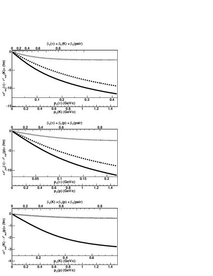
Figure 35: Separation between the average emission point of pions, kaons and protons in the pair rest frame along the pair transverse velocity. The values of the blast-wave parameters are for a round source, as listed in Table 1. Dot line: time shift in the laboratory boosted to the pair rest frame, dash line: spatial shift in the laboratory boosted to the pair rest frame, plain line: total spatial shift in the pair rest frame.

The average values of $x$ and $y$ will vary with particle mass and particle transverse velocity, which yields separations between pions and kaons, pions and protons, and protons and kaons in the pair rest frame shown as in Figure 35. The dashed and dotted lines show the contribution of the spatial ($\Delta r_{out}$) and time ($\Delta t$) separation boosted to the pair rest frame along the pair transverse momentum, respectively. i.e. the dash line shows $\langle\gamma_{T}\Delta r_{out}\rangle$ and the dot line represents $-\langle\gamma_{T}\beta_{T}\Delta t\rangle$. The plain line shows $\langle\Delta r^{*}_{out}\rangle=\langle\gamma_{T}(\Delta r_{out}-\beta_{T}\Delta t)\rangle$, the spatial separation in the pair rest frame. When boosting to the pair rest frame, time and spatial shifts in the laboratory frame add up due to their opposite signs. The largest (smallest) shift is obtained when the mass ratio between both species is the largest (smallest), i.e. for pion-proton (kaon-proton) pairs.

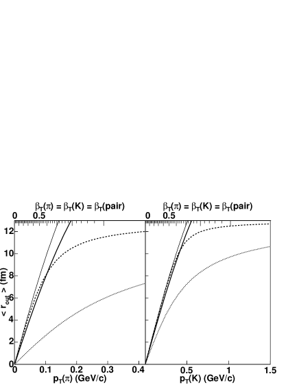
Figure 36: Average emission points of pions (left) and kaons (right) as a function of the pion and kaon velocity and momentum. All curve are calculated with $\rho_{0}$ = 0.9 and $\rho_{a}$ =0. The parameters $\tau$ and $\Delta t$ are irrelevant. Thin plain line: $R_{x}=R_{y}$ = 13 fm, T=0 GeV. Thick plain line: infinite system (i.e. $\Omega(r,\phi_{s})$ = 1 ), T = 0.1 GeV. Dash line: $R_{x}=R_{y}$ =13 fm, T=0.01 GeV. Dot line: $R_{x}=R_{y}$ =13 fm, T = 0.1 GeV.

In order to understand the behavior of $\Delta r^{*}_{out}$, it is instructive to investigate how the average emission points in the laboratory frame ($\langle r_{out}\rangle$) of pions and kaons behave in various conditions as shown in Figure 36. This figure shows the average emission points of pions and kaons in four different configurations: (1) The thin plain line shows the flow profile, (Equation 4), which sets the emission point of particles when T = 0 GeV. (2) the dot line is calculated assuming an infinite system, i.e. $\Omega(r,\phi_{s})=$ 1 and with $T=0.1$ GeV. (3) the dash line corresponds to a finite system as in Equation 1, with $a_{s}=$ 0, and (for illustration) an extremely low temperature, $T=0.01$ GeV. (4) the thick plain line is calculated using the standard parameters used in Figure 36. Only in case (1) are pions and kaons emitted exactly at the same point. Since $T=0$ GeV, all particles are always emitted at the same point as set by the flow profile. In case (2), particle emission points spread around the average emission defined by the flow profile. At small $\eta$ there are as many particles emitted at large $r$, i.e. large $\rho$ as at small $r$. But when $|\eta|$ is large, the term $e^{-m_{T}/Tcosh\rho(r,\phi_{s})cosh(\eta)}$ in Equation II.3 favors small $\rho$, i.e. small $r$. Thus, the average emission point $\langle r_{out}\rangle$ is smaller than the one defined by the flow profile. In case (3), the average emission points of pions and kaons follow closely the flow profile when the particle rapidity is significantly smaller than $\rho_{0}$. Close or beyond $\rho_{0}$, a certain fraction of the particle emission function is truncated due to the system finite size. The particle emission points are not allowed to spread beyond the system boundary, hence breaking the balance between particle emitted at small radii and particle emitted at large radii. Thus, the particle average emission radius is smaller than the emission radius given by the flow profile. Because the temperature is rather small, the average emission points of both species converge rapidly toward the radius of the system. The larger temperature in case (4) makes the average emission radii converge slowly toward the system limit. This phenomenon, with the addition of the phenomenon described in case (2) reduces very significantly the average particle emission radius compared to the flow profile limit.

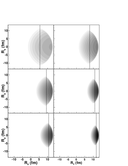
Figure 37: Distribution of the emission points in the transverse plane, for different particle species emitted at the same velocity, $\beta_{y}=0$ and $\beta_{x}=$ 0.907 on the left-hand side and $\beta_{x}=$ 0.974 on the right hand side. Top panels are for pions, middle for kaons and bottom for protons. The same logarithmic color scale is used for all six panels. The blast-wave parameters are the same as in Figure 36 except that $a_{s}=0.01$ The dashed lines show $\langle x\rangle$.

The effect of temperature depends on particle mass and momentum. Random smearing is maximal for particles with low mass and momentum such as the low $p_{T}$ pions that are usually associated with kaons or protons in non-identical particle correlation analyses. This effect is illustrated in Figure 37. It shows the probability of emitting pions at a given point in the transverse plane for two different pion momenta $\overrightarrow{p}=(0.15,0,0)$ and $\overrightarrow{p}=(0.3,0,0)$. Kaon and proton momenta are calculated so that they have the same velocities as pions. The region of the system that emits particles of a given momentum shrinks and moves towards the edge of the system as the particle mass, and/or momentum increases. The magnitude of the inward radius shift depends on the fraction of the source distribution that is truncated due to the system finite size. Thus, the inward shift of the average emission radius scales with the source size. This effect yields the systematic shift between the average emission points of pions, kaons and protons as shown in Figure 35 since pion source size is the largest and proton the smallest. Light particles are emitted the closer to the center of the source than heavier ones.

In addition to a spatial separation, the blast-wave parameterization induces a time shift between different particle species emitted at the same velocity as shown by the dot line in Figure 35. Due to random motion, the space-time rapidity ($\eta$) spreads around the momentum rapidity (Y). Because the relationship $t=\tau\cosh(\eta)$ is positive definite, the larger dispersion of $\eta$ for pions than for kaons or protons leads to a delay of the emission of pions with respect to kaons or protons. Protons are emitted first, then kaons and then pions. The spatial and time shifts have opposite signs in the laboratory frame but they sum up when boosting to the pair rest frame. The plain line in Figure 35 shows the added contributions of both shifts. The pion-kaon and pion-proton separation in the pair rest frame ranges from 5 to 15 fm, while the separation between kaons and protons is on the order of 2-4 fm. These shifts are large enough to be measured.

The curves on Figure 35 have been obtained by setting the blast-wave parameters to arbitrary values. We will now investigate how changing these parameters affects the shift between pions and kaons. The results obtained studying pion-kaon separation can be easily extrapolated to pion-proton and kaon-proton separations. Since experimental analyses of non-identical two-particle correlations performed to date do not investigate the azimuthal dependences with respect to the reaction plane, we will focus our study on central collisions. We will then show that the shift between the average emission points of different particle species oscillates with respect to the reaction plane without investigating the effect of varying the parameters in detail.

III.4.2 Non-identical particle correlations in central collisions

In central collisions, azimuthal symmetry implies that the particle emission pattern depends only on the relative angle between the position and momentum $\phi_{p}-\phi_{s}$. Thus, setting for convenience $\phi_{p}=0$, yields:

$$\langle r^{*}_{out}(i)\rangle = \langle\gamma_{T}(x_{i}-\beta_{T}\Delta t_{i})\rangle$$ (42)

$$\langle r^{*}_{side}(i)\rangle = 0$$ (43)

Furthermore, we consider emission from an azimuthally-isotropic source ($R_{x}=R_{y}$ and $\rho_{2}=0$) only. Hence, the only quantity of interest is $\langle\Delta r^{*}_{out}\rangle$.

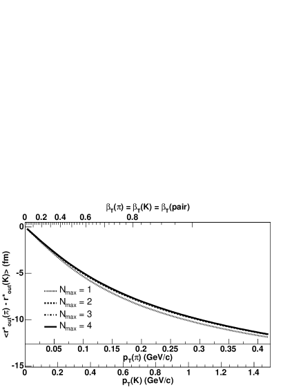
Figure 38: Average separation between $\pi$ and K in the pair rest frame as a function of the pion and kaon momentum using several values of $N$, the maximum value of $n$ taken in the summation of Equation II.3. Values of the blast-wave parameters are for a round source, as listed in Table 1.

Figure 38 shows the dependence of the average separation between $\pi$ and K in the pair rest frame as a function of the pion and kaon momentum using several values of $N$, the maximum value of $n$ taken in the summation of Equation II.3. Pions and kaons are of course treated as bosons. The difference between the average separation calculated either by using a Boltzman function (N=1) or by approximating the Bose-Einstein distribution at the $4^{th}$ order is smaller than 0.5 fm. The maximum relative difference is on the order of 8% at small transverse momentum. The Bose-Einstein distribution already converges when N=2.

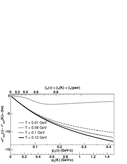
Figure 39: Average separation between $\pi$ and K in the pair rest frame as a function of the pion and kaon momentum for different temperature. The values of the other blast-wave parameters are for a round source, as listed in Table 1.

Figure 39 shows the dependence of the spatial shift between pions and kaons in the pair rest frame as a function of the pair velocity for different temperature. The shift increases as the temperature increases all the way from 0.01 GeV to 0.12 GeV. When the temperature is very low (e.g. 0.01 GeV), pion and kaon emission patterns are dominated by space-momentum correlation independent of particle masses. In the limit of zero temperature, there is a unique correspondence between particle velocity and emission point. In that case since we consider particles with the same velocity, pions and kaons are emitted from the same point. On the other hand when the temperature is non zero, a fraction of the pions and kaons that would be emitted in a infinite system are truncated, which shifts their average emission points inward. Because the pion source size is significantly larger than the kaon source size due to the pion lower mass and momentum, the pion average emission point is more shifted inward than kaon’s, which is illustrated in Figure 40. This figure shows the contribution of the spatial shift in the average separation between the pion and kaon average emission points in the pair rest frame. When the temperature is low (0.01 GeV), both spatial and time separation are small as shown by the dash lines in figures 40 and  41. As the temperature increases, the pion emission time increases faster than the kaon emission time; the higher the temperature the larger the shift between pion and kaon average emission time (after boosting into the pair rest frame). On the other hand the spatial shift varies little within the temperature range expected in relativistics heavy-ion collisions (0.08-0.12 GeV). At temperature above 10 MeV/c, a fraction of the pion and kaon sources is truncated even at low particle velocity. The fraction of the source that is truncated, which leads to an inward shift of the average emission radius, varies with transverse momentum and particle mass but it is relatively insensitive to temperature variation between 0.08 and 0.12 GeV. It is interesting to note that the average spatial separation between pion and kaon in the laboratory frame actually decreases as the particle velocity rises above 0.8c. However, this decrease is not visible in Figure 39 and  40 becayse the $\gamma_{T}$ factor applied when boosting to the pair rest frame rises faster with velocity than the separation between pions and kaons in the laboratory frame decreases.

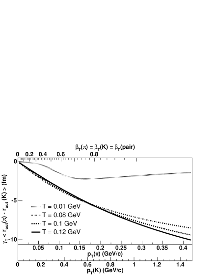
Figure 40: Contribution of the spatial shift to the average separaration between pions and kaons in the pair rest frame as a function of the pion and kaon momentum for different temperature. The values of the other blast-wave parameters are for a round source, as listed in Table 1.

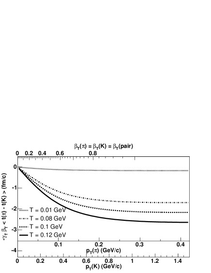
Figure 41: Contribution of the time shift to the average separaration between pions and kaons in the pair rest frame as a function of the pion and kaon momentum for different temperature. The values of the other blast-wave parameters are for a round source, as listed in Table 1.

Changing the maximum flow rapidity ($\rho_{0}$) also affects the separation between pions and kaons in the pair rest frame as shown in Figure 42. When $\rho_{0}=0$, pions and kaons are emitted from the same space point as shown on Figure 43 and only the time shift remains (Figure 44). Indeed, the time shift depends weakly on $\rho_{0}$. Figure 44 shows that the contribution of the time shift to the separaration between pions and kaons in the pair rest frame reaches a plateau when the pion momentum reaches 0.25 GeV/c. The magnitude of the time shift starts decreasing in the laboratory frame upon reaching this pion momentum but it is compensated by an increase of the boost factor $\gamma_{T}\beta_{T}$. On the other hand, when $\rho_{0}$ is large enough, a significant spatial separation appears in the pair rest frame, which is sensitive to the value of $\rho_{0}$. The main effect of increasing the flow strength is to decrease the pion (and kaon) transverse source size, as shown in Figure 31. In the laboratory frame, the spatial shift between pion and kaon average emission point switches from decreasing to increasing as the particle velocity increase. The value of the velocity where this switch occurs, depends on the value of $\rho_{0}$. The increase of the spatial shift between pions and kaons arises from two effects: the first is the expected shift of the average emission point of both particles due to the flow profile; the second is that the kaon source size drops more rapidly than the pion source size. Then, above a velocity that depends on $\rho_{0}$, the fraction of pion that would be emitted beyond the system limit starts dropping faster than the corresponding fraction of kaons, thus the separation between the average emission points of pions and kaons decreases. However, this turn over, which takes place in the laboratory frame is not directly visible in Figure 43 because the boost factor $\gamma_{T}$ compensates it.

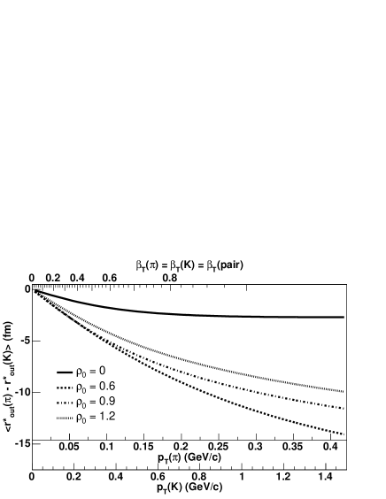
Figure 42: Average shift between the pion and kaon emission point in the pair rest frame as a function of the pion and kaon momentum for different flow rapidity ($\rho_{0}$) The values of the other blast-wave parameters are for a round source, as listed in Table 1.

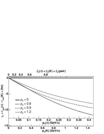
Figure 43: Contribution of the spatial shift to the average separaration between pions and kaons in the pair rest frame as a function of the pion and kaon momentum for different flow rapidity ($\rho_{0}$) The values of the other blast-wave parameters are for a round source, as listed in Table 1.

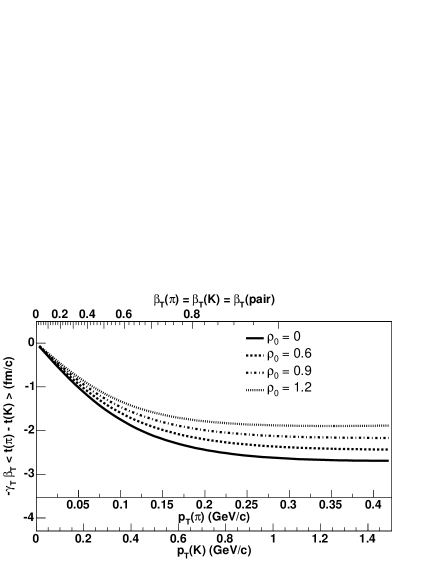
Figure 44: Contribution of the time shift to the average separaration between pions and kaons in the pair rest frame as a function of the pion and kaon momentum for different flow rapidity ($\rho_{0}$) The values of the other blast-wave parameters are for a round source, as listed in Table 1.

Figure 45 shows the sensitivity of the average separation between pion and kaon emission point in the pair rest frame to varying the system radius. This spatial separation scales directly with the system radius because it does not modify the fraction of pions or kaons that are truncated due to the system finite size.

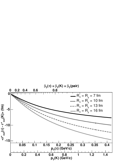
Figure 45: Average shift between the pion and kaon emission point in the pair rest frame as a function of the pion and kaon momentum for different system radius ($R_{x}=R_{y}$). The values of the other blast-wave parameters are for a round source, as listed in Table 1.

Like the system radius, the proper life time $\tau_{0}$ acts as a scale driving the shift between pion and kaon emission time. Figure 46 shows the effect of varying $\tau_{0}$ on the separation between pion and kaon in the pair rest frame. The effect of varying $\tau_{0}$ is small because the contribution of the time shift to the separation in the pair rest frame is significantly smaller than the contribution of the spatial separation.

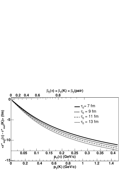
Figure 46: Average shift between the pion and kaon emission point in the pair rest frame as a function of the pion and kaon momentum for different system proper life time ($\tau_{0}$). The values of the other blast-wave parameters are for a round source, as listed in Table 1.

Figure 47 shows the effect of varying $a_{s}$ on the separation between pion and kaon in the pair rest frame. Unlike in Figure 34, $\rho_{0}$ was kept constant. Indeed varying $\rho_{0}$ significantly affects the average emission radii, which hides the effect of changing $a_{s}$ at low velocity. However, when the velocity is larger than $\tanh(\rho_{0})=0.716c$, the amount of boost and space-momentum correlation than particle acquire depends on $a_{s}$; the larger $a_{s}$ the larger the boost. Thus, when the pair velocity is lower than $0.716c$, the separation decreases with increasing $a_{s}$ because the fraction of truncated particles decrease. When the pair velocity is larger than $0.716c$, increasing $a_{s}$ has the same consequence as increasing $\rho_{0}$.

Figure 47: Average shift between the pion and kaon emission point in the pair rest frame as a function of the pion and kaon momentum for surface smoothness ($a_{s}$). The values of the other blast-wave parameters are for a round source, as listed in Table 1.

III.4.3 Non-identical particle correlations in non-central collisions

As reported in ref PRLNonId , the average space-time separation between different particle species may depend on the particle emission angle with respect to the reaction plane. The effect in the blast-wave parameterization is shown in Figure 48. The blast-wave parameters are the same as in Figure 35 with the exception of $R_{x}$ and $\rho_{2}$ which are varied. Clear oscillations of $\langle r^{*}_{out}(\pi)-r^{*}_{out}(K)\rangle$ are found when $R_{x}$ is set to 11 fm, i.e. when the source is out-of-plane extended ($R_{y}=$ 13 fm). Small oscillations of $\langle r^{*}_{side}(\pi)-r^{*}_{side}(K)\rangle$ appear as well. The oscillations in both directions are on the order of 1-2 fm, which may be measurable. On the other hand, keeping the source cylindrical but setting the flow modulation parameter $\rho_{2}$ to 0.05 yields very small oscillations, which will be very challenging to probe experimentally. Thus, non-identical two particle correlation analyses with respect to the reaction plane, as pion HBT may provide a good handle on the source shape but not on the flow modulation.

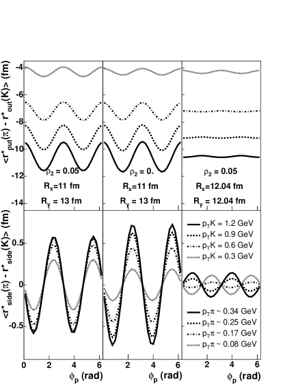
Figure 48: Average separation between pions and kaons in the pair rest frame as a function of their momentum azimuthal angle with respect to the reaction plane. The four different lines are calculated for 4 different kaon momenta and the corresponding 4 different pion momenta required so that pions and kaons have the same velocity. The values of the blast-wave parameters used in the left panel are for a ”non-round” source, as listed in Table 1 . The same parameter were used in the middle panel except that $\rho_{2}=0$. The round source parameters are used in the right panel except that $\rho_{2}=0.05$. The separation along the $out$ and $side$ axes are shown on the upper and lower panel respectively.

III.5 Summary of effects of parameters

Above, we have explored the sensitivity of several experimental observables on various freezeout parameters. Here, we summarize in an orthogonal manner– describing briefly the main observable effects due to an increase in each parameter, if the other parameters are left fixed.

The temperature parameter $T$ quantifies the randomly-oriented kinetic energy component of the freezeout scenario. Increasing this energy component leads to decreased slopes of $p_{T}$ spectra, especially for light-mass particles. Since random motion destroys space-momentum correlations, increasing $T$ reduces measured elliptic flow ($v_{2}$) and increases homogeneity scales, i.e. $R^{2}_{\mu,{0}}$. On the other hand, for the range of values considered, increasing temperature increases the average separation in the pair rest frame between pions and heavier particles, e.g. $\langle r^{*}_{out}(K)-r^{*}_{out}(\pi)\rangle$.

The $\phi$-averaged transverse flow strength is quantified in this model by $\rho_{0}$. Increasing this directed energy component decreases slopes of $p_{T}$ spectra, especially for heavier particles. Increasing $\rho_{0}$ leads to increasing space-momentum correlations, which reduce $R^{2}_{\mu,{0}}$ and $\langle r^{*}_{out}(K)-r^{*}_{out}(\pi)\rangle$, and at constant $\rho_{2}$ reduces $v_{2}$ at high $m_{T}$.

The parameter $a_{s}$ quantifies the “surface diffuseness” of the spatial density profile. Taking care to keep the average transverse flow fixed, variation in $a_{s}$ has little effect on purely momentum-space observables: $p_{T}$ spectra and $v_{2}(m,p_{T})$. On the other hand, going from a “box profile” ($a_{s}=0$) to a pseudo-Gaussian profile ($a_{s}=0.3$) increases the “out-to-side” ratio $R^{2}_{o,{0}}/R^{2}_{s,{0}}$ at higher $p_{T}$, as the homogeneity region is not constrained by hard geometric “emission boundaries.” Furthermore, for a fixed average transverse flow (and flow gradient), increasing $a_{s}$ leads to stronger oscillations in the HBT radius parameters. Increasing $a_{s}$ also increases the $\langle r^{*}_{out}(K)-r^{*}_{out}(\pi)\rangle$ when the temperature and particle velocity are such that the pion source size is significantly larger than the kaon’s.

Considering variations in the geometric transverse scale of the source $\sqrt{R_{x}^{2}+R_{y}^{2}}$, while keeping all else (including $R_{y}/R_{x}$) constant, we conclude that the sensitivity is in the HBT radii and the average separation between different particle species. In HBT, the sensitivity to this parameter is through $R^{2}_{o,{0}}$ and $R^{2}_{s,{0}}$. The spatial shifts that contribute to the separation $\langle r^{*}_{out}(K)-r^{*}_{out}(\pi)\rangle$ in the pair rest frame scales directly with this parameter. Momentum-space observables such as spectral shapes or $v_{2}$ are unaffected.

We turn now to variations in the timescale parameters– the evolution duration ($\tau_{0}$) and emission duration ($\Delta\tau$). The only significant variations are in $R^{2}_{l,{0}}$ and $R^{2}_{o,{0}}$, and these depend differently on $\tau_{0}$ and $\Delta\tau$, allowing independent probes of the two parameters. The time shifts that contribute to the separation $\langle r^{*}_{out}(K)-r^{*}_{out}(\pi)\rangle$ in the pair rest frame scales directly with these parameters ($\tau_{0}$ and/or $\Delta\tau$).

Non-central collisions may exhibit azimuthally anisotropic geometry and/or dynamics in the freeze-out configuration. These two effects were studied by varying $R_{y}/R_{x}$, and $\rho_{2}$, respectively. Azimuthally-integrated $p_{T}$ spectra were negligibly affected, as were the $\phi_{p}$-averaged values of HBT radii ($R^{2}_{\mu,{0}}$). Observables designed to probe anisotropy, $v_{2}$ and $R^{2}_{\mu,{2}}$ of course showed strong sensitivity to geometric or dynamical anisotropy, increasing strongly in magnitude as $R_{y}/R_{x}$ deviates from unity and/or $\rho_{2}$ from zero.

IV Comparison with existing data

In the previous section, we reviewed the various experimental observables that the blast-wave parameterization may be able to reproduce. The effect of changing blast-wave parameters has been examined. In this section, we investigate how well those parameters can be constrained by the experimental data.

Before comparing the blast-wave parameterization with data, we highlight its limitations and possibly not valid assumptions:

• Freeze-out from a thermalized system at a constant temperature. In the blast wave framework, freeze-out is assumed to take place at the same temperature for every particle. In principle, this condition may be relaxed by fitting separately the data for each type of particle. (We do not attempt this here.) Perhaps a more important assumption, however, is made in discussing “temperature” at all; it requires system thermalization. If particles are emitted in a non-thermal way our framework may fail to describe the data.

• Longitudinal boost invariance. The blast wave parameterization relies on longitudinal boost invariance. Elliptic flow data ($v_{2}$) published by the PHOBOS collaboration clearly show that longitudinal boost invariance is broken for rapidity larger than 1 PhobosV2 . Thus the blast wave parameterization can only be applied within $|Y|<1$. This assumption will be validated or ruled out by high precision data.

• No resonances. The observables that constrain the blast wave are calculated for each particle species using their own masses, ignoring the fact that some particle may be decay products of other particles. In fact a large fraction of pions and protons produced at RHIC energy originate from resonance decays. As mentioned in section 3, pions from $\omega$ meson decay distort the pion source space-time distribution but this effect is limited because the fraction of pions coming from $\omega$ is on the order of 10%. On the other hand, pion spectra and to a lesser extent proton spectra may be significantly distorted by resonance feed-down. Within the blast wave framework however, it was found in Peitzmann ; STARSpectra200 that accounting for resonances affects the Blast Wave parameters extracted fit to spectra by no more than 20%. While 20% is not negligeable, we feel that the gross features of the parameterization are preserved. On the other hand, an investigation of the effect of resonance feed-down on $v_{2}$ remains to be performed.

We focus on data from Au-Au collisions at $\sqrt{s_{NN}}=$ 130 GeV published by the PHENIX and STAR collaborations at RHIC. The measurements used are listed on top of Table 2. To avoid uncertainties between different experiments and to optimize the overlap between centrality bins, we do not use the full set of data published at RHIC. Three centrality bins are available. The approximate overlap between the centrality bins for the different measures may affect the quality of the fits.

	Central	Mid-central	Peripheral
data
$\pi$, K, p spectra PhenixSpectra130	0-5%	15-30%	60-92%
$\Lambda$ spectra StarLaSpectra130	0-5%	20-35%	35-75%
pion radii  STARHBT	0-12%	12-32%	32-72%
Elliptic flow  STARv2ID	0-11%	11-45%	45-85%
$\chi^{2}/$(# data points)
$\pi^{+}$ & $\pi^{-}$ spectra	7.2/10	26.5/10	13.0/9
$K^{+}$ & $K^{-}$ spectra	24.2/22	21.4/22	10.1/10
$p$ & $\overline{p}$ spectra	10.6/18	23.2/18	28.0/12
$\Lambda$ & $\overline{\Lambda}$ spectra	9.5/16	12.8/16	11.0/16
$\pi$ $v_{2}$	14.6/12	29.8/12	5.2/12
$p$ $v_{2}$	1.6/3	9.2/6	0.8/3
$\pi$ $r_{out}$	1.9/6	0.4/2	0.4/2
$\pi$ $r_{side}$	2.7/6	0.07/2	0.06/2
$\pi$ $r_{long}$	5.3/6	0.003/2	0.1/2
Total	77.6/99	107.7/90	68.7/68
parameters
T (MeV)	106 $\pm$ 3	107 $\pm$ 2	100 $\pm$ 5
$\rho_{0}$	0.89 $\pm$ 0.02	0.85 $\pm$ 0.01	0.79 $\pm$ 0.02
$\langle\beta_{T}\rangle$	0.52 $\pm$ 0.01	0.50 $\pm$ 0.01	0.47 $\pm$ 0.01
$\rho_{2}$	0.060 $\pm$ 0.008	0.058 $\pm$ 0.005	0.05 $\pm$ 0.01
$R_{x}(fm)$	13.2 $\pm$ 0.3	10.4 $\pm$ 0.4	8.00 $\pm$ 0.4
$R_{y}(fm)$	13.0 $\pm$ 0.3	11.8 $\pm$ 0.4	10.1 $\pm$ 0.4
$\tau(fm/c)$	9.2 $\pm$ 0.4	7.7 $\pm$ 0.9	6.5 $\pm$ 0.6
$\Delta t(fm/c)$	0.003 $\pm$ 1.3	0.06 $\pm$ 1.3	0.6 $\pm$ 1.8

Table 2: Upper section: data used in the fit. Middle section: number of $\chi^{2}/$ data points for each measure. Lower section: best fit parameters. Note that $\langle\beta_{T}\rangle$ is not a fit parameter, but it is calculated from $\rho_{0}$.

The blast-wave parameters are constrained by simultaneously fitting transverse momentum spectra, transverse momentum azimuthal anisotropy ($v_{2}$), and pion HBT radii. Bose-Einstein and Fermi-Dirac distribution are used when appropriate using the approximation to the 4${}^{t}h$ order as in Equation II.3, i.e. the value of $n=4$ in the summation of Equation II.3. The quality of the fit to each measure is shown by the $\chi^{2}$ per data points listed in Table  2. The number of degrees of freedom is not shown because the number of parameters cannot be subtracted from the number of data points independently for each measure. In addition to the 7 blast-wave parameters, there are 8 scaling parameters used to normalize $\pi^{+}$, $\pi^{-}$, $K^{+}$, $K^{-}$, $p$, $\overline{p}$, $\Lambda$, and $\overline{\Lambda}$ spectra. These scaling parameters ($A$) are not minimized by the fitting function but calculated directly. The $\chi^{2}$ for a given spectra is given by:

$$\chi^{2}=\sum_{i}(\frac{d_{i}-Ac_{i}}{e_{i}})^{2}$$ (44)

$d_{i}$ is the measured invariant yield in the bin $i$. $e_{i}$ is the experimental error on $d_{i}$, and $c_{i}$ is the calculated invariant yield. The $\chi^{2}$ minimum occurs when $d\chi^{2}/dA$ = 0, hence:

$$A=\frac{\sum_{i}{d_{i}c_{i}/e_{i}^{2}}}{\sum_{i}{c_{i}/e_{i}^{2}}}$$ (45)

To avoid the region where resonance feed-down may be large and where the Boltzmann approximation may not be valid, fits to transverse momentum spectra are restricted to pions with $p_{T}>0.4$ GeV/c. We further restrict the fit range to $p_{T}<1$ GeV/c for pions, $p_{T}<1.5$ GeV/c for kaons, $p_{T}<2$ GeV/c for protons and lambdas, because hard processes may significantly contribute to the particle yield above these momenta PeitzmannBWHighPt .

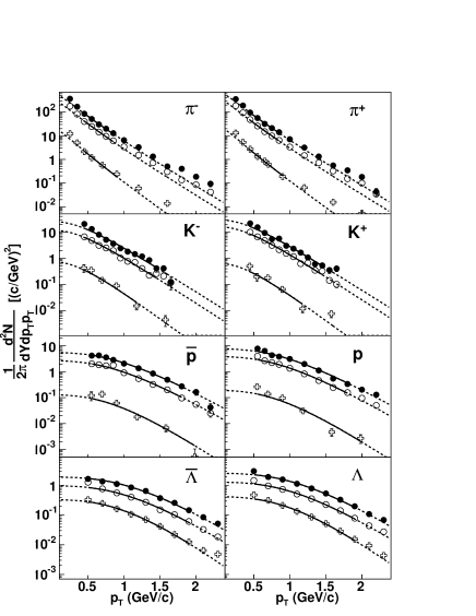
Figure 49: Comparison of the data with the blast-wave calculations performed with the best fit parameters in three centrality bins. The closed circles are central data, the open circles are mid-central data and the crosses are peripheral data. The plain lines show the blast wave calculation within the fit range while the dash lines show the extrapolation over the whole range.

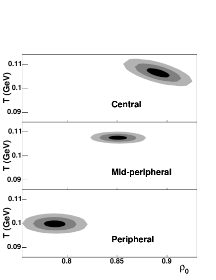
Figure 50: Number of $\sigma$ contour of the maximum flow rapidity ($\rho_{0}$) with respect to the temperature (T). The shadows show the 1, 2 and 3 $\sigma$ contours from darkest to lightest.

Given the large number of data points from spectra, the temperature (T) and the maximum flow rapidity ($\rho_{0}$) parameters are constrained by transverse mass spectra. A comparison of data and the blast-wave calculation with the best fit parameters is shown in Figure 49. In semi-logarithmic plots, the data and the model fits seem to agree very well. The $\chi^{2}$/(# data points) in Table 2 show, however, that the fit quality varies between particle species and centrality bins. The correlation between the flow rapidity and temperature is shown in Figure 50. The extracted temperatures and flow velocities are consistent with similar studies reported in Ref. BurwardHoy ; Peitzmann ; Tomasik ; NuKanetaQM01 . The differences between these analyses are due to the use of different data sets, different fit ranges, and different flow and spatial profiles. The study reported in Ref. Peitzmann shows that accounting for resonance feed-down leads to a temperature 30% higher and a transverse velocity 15% lower than in our study.

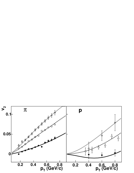
Figure 51: Comparison of the $v_{2}$ data with the blast-wave calculations performed with the best fit parameters in three centrality bins. The closed circles are central data, the open circles are mid-central data and the crosses are peripheral data.

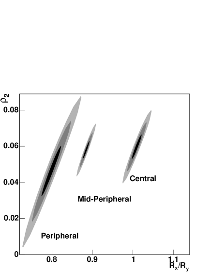
Figure 52: Number of $\sigma$ contours of the ratio of the in-plane radius over the out-of-plane radius ($R_{x}$/$R_{y}$) with respect to the flow rapidity oscillation parameter ($\rho_{2}$). The colors show the 1, 2 and 3 $\sigma$ contours from darkest to lightest.

The fit of $v_{2}$ mainly constrains the flow rapidity modulation parameter, $\rho_{2}$, and the ratio between the radius in-plane and out-of-plane, $R_{x}/R_{y}$. A comparison between the data and the blast-wave calculation with the best fit parameters is shown in Figure  51. The correlation between $\rho_{2}$ and $R_{x}/R_{y}$ is shown in Figure 52. The fit performed in this paper differs from the fit reported together with the data in Ref. STARv2ID . There are three main differences: (i) in Ref. STARv2ID , the temperature and flow velocity are free parameters while in this paper they are mostly determined by spectra shapes, (ii) a filled volume and a flow profile are used instead of a shell, (iii) the fits are performed on three centrality bins instead of the minimum bias sample. Thus, a direct comparison between the fit parameters extracted in this paper and those reported in Ref. STARv2ID is difficult. The freeze-out spatial anisotropy probed by the ratio $R_{x}/R_{y}$, increases when increasing the initial state spatial anisotropy, $i.e.$ when going from central to peripheral events. The flow modulation decreases from central to peripheral events, following the same trend as $\rho_{0}$.

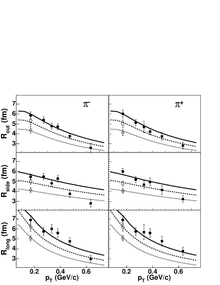
Figure 53: Comparison of the pion source data measured by the STAR (circle) and the PHENIX (box) collaborations with the blast-wave calculations. Only the STAR data were used to constrain the blast-wave parameters. The closed circles are the central data, the open circles are the mid-central data and the crosses are peripheral data.

The pion source radii allow us to estimate the parameters $R_{x}$ (or $R_{y}$), $\tau$ and $\Delta t$. As discussed earlier, the ratio $R_{x}/R_{y}$ is constrained by the fit to $v_{2}$. In the mid-peripheral and peripheral bins, the pion source size has been measured at only one transverse momentum, which weakly constrain the parameters. The comparison between the data and the blast-wave calculation performed with the best fit parameters is shown in Figure 53. This figure includes the pion source radii reported by the PHENIX collaboration PhenixHBT although they weren’t used in the fit. These radii were measured over the 30% most central events, which doesn’t overlap well with the STAR collaboration centrality bins (0-12%, 12-32% and 32-72%). Qualitatively the PHENIX data points agree with the blast-wave fit as they oscillate between the central and mid-peripheral lines. The $\chi^{2}$ obtained from the fit is small, because the systematic errors were added in quadrature to the statistical errors. The system radius increases from peripheral events to central events following the growth of the system initial state. The final system radius is roughly twice the initial system radius, which is a clear evidence of the system expansion. The proper time ($\tau$) is surprisingly small. Typically, hydrodynamical calculations reach kinetic freeze-out in 15 fm/c, not 9 fm/c KolbLatest . The hydrodynamical calculations may be over-predicting the system life-time or the assumption underlying the extraction of $\tau$ may not be valid. The assumption of a boost invariant expansion along the beam axis from a narrow (less than 1 fm thick) pancake may be too simplistic. Indeed, it has been shown that accounting for the fluid viscosity breaks the boost invariant flow TeaneyViscosity . Furthermore, three dimensional hydrodynamical calculations reproduce the measured pseudo-rapidity distribution only when the initial width of the system along the beam axis extends over several units of spatial pseudo-rapidity Hirano3D . Such initial conditions lead to a longitudinal expansion that also breaks boost invariant scaling. In these calculations, even though the system persists for 15 fm/c, the $R_{long}$ radii is well reproduced. Thus, the absolute value of proper life-time, $\tau$, extracted within the blast-wave parameterization may be questionable. Along the same lines, the very short emission duration is surprising. Indeed, a scenario where particles are emitted in a flash would appear rather unlikely. (On the other hand, processes such as supercooling CsorgoCsernaiFlash have been discussed, and may lead to such a scenario.) Recent experimental data  MercedesQM02 show that the value of the $R_{out}$ radius may have been underestimated by the experiments. Thus, since the emission duration parameters $\Delta t$ strongly depends on $R_{out}$, it is not appropriate to draw definite conclusions until the experimental issues are settled.

Figure 54: Oscillations of the pion source radii obtained with the best fit parameters in the three centrality bins.

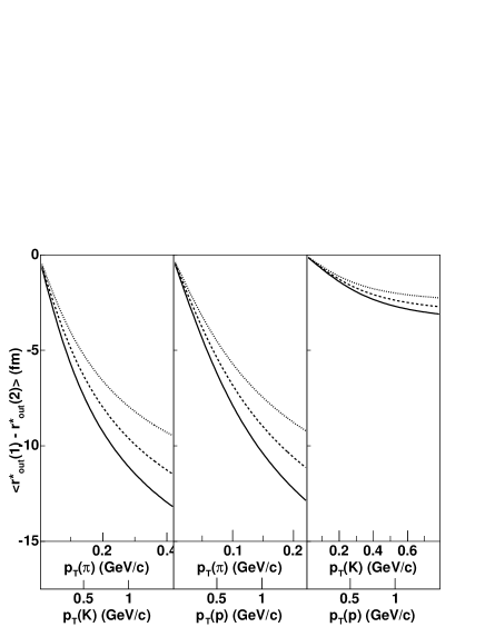
Figure 55: Space-time separation between pions and kaons (left), pions and protons (middle) and kaons and protons (right) calculated with the best fit parameters in the three centrality bins. Plain line: parameters from fit to central data. Dash line: parameters from mid-peripheral data. Dotted line: parameters from fit to peripheral data.

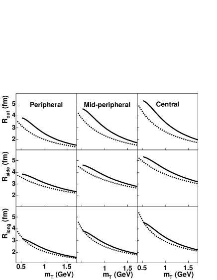
Figure 56: Kaon source radii (plain line) compare to the pion radii (dash line). The blast-wave calculation are performed with the best fit parameters in each centrality bins.

We have shown that $\pi$, K, p, $\Lambda$ transverse momentum spectra, $\pi$, p elliptic flow, and pion source radii measured in Au-Au collisions at $\sqrt{s_{NN}}=$ 130 GeV are well reproduced by the blast-wave parameterization. With the exception of the time-scale parameters (system proper life time and emission duration), which fall short of any realistic model calculations, the fit parameters are within expectations. This issue may be resolved when new data on pion source radii become available. Based on the published data in Au-Au collisions at $\sqrt{s_{NN}}=$ 130 GeV, we conclude that the blast-wave parameterization provides a good description of the system freeze-out stage.

This conclusion will be tested in the future, using the sensitivity of the blast-wave parameterization to observables that have been presented in the previous section: the oscillation of the pion radii with respect to the reaction plane, and the space-time separation between the emission points of different particle species. Using the parameters extracted from the fits we have calculated the corresponding oscillation of the pion radii with respect to the reaction plane (Figure 54) and the separations between the average space-time emission point of pions kaons and protons (Figure 55). We have also calculated the kaon source radii as shown in Figure 56 since they may become available from the RHIC experiments MercedesQM02 ; PHENIXHBTQM02 . The blast-wave parameterization faces the challenge of simultaneously reproducing a large variety of observables that will be measured in Au-Au collisions at 200 GeV, namely: (1) pion, kaon, proton and $\Lambda$ transverse momentum spectra, (2) the elliptic flow of many particle species, (3) the pion source radii including the oscillations with respect to the reaction plane, (4) the kaon source radii, (5) the space-time separation between pion, kaon and proton sources. If a satisfactory agreement between these various measurements is achieved, it would provide evidence of a collective expansion that would be very challenging to avoid. Furthermore, when high quality data becomes available that allows for separate fits to each particle species, the blast-wave parameterization may prove to be an important and handy tool to assess whether or not the freeze-out time depends on the hadronic cross-sections. It will be especially interesting to study particles with presumably low hadronic cross sections such as the $\phi$, $\Xi$, $\Omega$. Since these particles may not be sensitive to hadronic collectivity, they may have a higher freeze-out temperature, they may pick up less collective flow, and freeze-out earlier and from a smaller system than $\pi$, K, p, $\Lambda$. It may be possible to distinguish between the collective expansion at the partonic (if any) versus hadronic stage.

V Summary and Outlook

We have discussed a scenario of particle kinetic freeze-out in heavy ion collisions, inspired by the results of full hydrodynamic calculations of the collision evolution. The scenario, while simplified, nevertheless includes several important features which drive experimental observables of the bulk properties of the system. This includes random (“thermal”) motion superimposed upon collective flow fields, an anisotropic transverse geometry, and a freeze-out distribution in proper time. The main assumptions of the model are: longitudinal boost-invariance; the same parametric source for all particle types (e.g. $\pi,p$); and the invariance of source parameters over the kinetic freeze-out process (or, equivalently, that the model source parameters can represent the appropriate average of the time-evolving parameter). We discussed the interplay of the various features, such as space-momentum correlations depending on the competition between thermal and collective motion and the source geometry.

The various features (e.g. random thermal motion) were quantified with several parameters (e.g. $T$) in a mathematical model outlined in Section 2. The general class of integrals which relate the model emission function to the various experimental observables was identified.

The sensitivity of several observables to the underlying physics represented by the parameters was studied by systematically varying each parameter in Section 3. In addition to momentum-space observables such as the $p_{T}$ spectra and elliptic flow, which have been discussed previously in the context of similar models, we focussed on the sensitivity of final-state correlations between non-identical particles and azimuthally-sensitive HBT, new coordinate-space-sensitive analysis tools now becoming available with the quality high statistics datasets from RHIC.

The non-trivial interplay between competing physics effects was different for the different observables. It is clear that the model parameter-space can only be constrained by examining several observables simultaneously; e.g. $p_{T}$ spectra alone are insensitive to the source shape ($R_{y}/R_{x}$) and only crudely distinguish between high transverse flow and high temperature. Furthermore, from Section 3, it is clear that experimental data can over-constrain the model parameter space. If consistency with $p_{T}$ spectra and HBT data demand a high temperature and small transverse boost velocity, this has inescapable consequences for $\pi-K$ correlations and elliptic flow. This allows for the “break-down” of the parametric model, and indicates the need to consider new driving physics effects.

In Section 4, the model was used as a functional form in a simultaneous fit to particle spectra ($\frac{dN}{dp_{T}}(p_{T},m)$), elliptic flow ($v_{2}(p_{T},m)$), and pion HBT ($R(p_{T})$) for three centrality classes from published RHIC results for Au-Au collisions at $\sqrt{s_{NN}}=130$ GeV. While higher-$p_{T}$ HBT radii from PHENIX are only qualitatively described, a good fit is obtained to the $p_{T}$ spectra, elliptic flow, and low-$p_{T}$ STAR HBT radii.

Most of the physical parameter values obtained from the fits, as well as their evolution with collision centrality, fall within reasonable expectations. The exceptions are the evolution duration $\tau_{0}$ and emission duration $\Delta\tau$, which are shorter than most physical models predict. The $\Delta\tau$ discrepancy may be partially resolved by an improved experimental treatment of the Coulomb interaction in HBT analyses; this will be evaluated upon publication of the new results from RHIC. The $\tau_{0}$ value is strongly connected to the model assumption of boost-invariance; if this assumption is invalid at mid-rapidity at RHIC (e.g. if there is longitudinal acceleration in the early system evolution), we expect our fit values to be only lower limits on the evolution duration.

Finally, Section 4 discusses expectations for kaon HBT, azimuthally-sensitive pion HBT, and emission space-time separations between non-identical particles ($\pi$, $K$, $p$), based on the fit parameters to the published data. Expectations for the azimuthally-sensitive pion HBT are driven by the elliptic flow data, which indicates $R_{y}>R_{x}$ (see Table 2)– i.e. the freeze-out system shape is out-of-plane extended, qualitatively similar to the geometrical overlap configuration in the entrance channel of the collision. From Section III.3, it is clear that this determines the phases (and amplitudes) of the expected oscillations in the HBT radii– i.e. the signs and magnitudes of $R^{2}_{\mu,2}$. If azimuthally-sensitive HBT measurements confirm this out-of-plane freeze-out configuration, it might provide further evidence of short evolution times $\tau_{0}$, since it would imply that the source, which is expanding faster in the reaction plane than out of it, did not have sufficient time to overcome its initial geometric anisotropy before freeze-out. Quantifying the timescale in this way is outside the scope of the blast-wave model, which does not attempt to describe the system evolution.

Exploration of simple parameterizations such as the blast-wave is driven by the desire to connect observations to driving underlying physics. Furthermore, a quantitative interpretation of many measurements (perhaps especially two-particle interferometry) requires some model assumptions. Naturally, one prefers assumptions which are consistent with other measurements (e.g. elliptic flow) in the same system. Especially since first-principle model calculations have difficulty consistently explaining the range of observations in the soft sector of RHIC, it is hoped that insight may be gained from rather simple theory-inspired parameterizations such as the blast-wave.

Inasmuch as such parameterizations reproduce observations, there is hope that the driving physics effects have been approximately quantified, and one may compare the “underlying” parameters (e.g. timescales) with first-principles calculations in an effort to isolate the cause of the discrepancy between such calculations and observation. On the other hand, when simplistic parameterizations cannot, with any set of parameters, reproduce the main features of the data, it indicates that something additional is driving observations. In parameterizations, features may be implemented and “turned on and off,” one at a time, testing for consistency with a range of experimental observations. The insight gained from such studies can then be fed back into more “theoretical” models. It is hoped that new experimental data will further constrain– or break– the simple parameterization, generating insights into the dynamics of heavy ion collisions at RHIC.

References

- (1)
- (2) For reviews and recent developments, see proceedings of the Quark Matter conferences: QM99 [Nucl. Phys. A661 (1999)]; QM01 [Nucl. Phys. A698 (2002)]; QM02 [Nucl. Phys. A715 (2003)].
- (3) E.V. Shuryak, Phys. Lett. B78 150 (1978).
- (4) E.V. Shuryak, Sov. J. Nucl. Phys. 28 408 (1978); J. Kapusta, P. Lichard, and D. Seibert, Phys. Rev. D44 2774 (1991).
- (5) BRAHMS Collaboration, Phys. Rev. Lett. 91 072305 (2003); PHENIX Collaboration, Phys. Rev. Lett. 87 052301 (2001); ibid, nucl-ex/0207009; ibid, Phys. Rev. Lett 91 072301 (2003); ibid, Phys. Rev. Lett 91 072303 (2003); ibid, nucl-ex/0308006; PHOBOS Collaboration, Phys. Rev. Lett. 91 072302 (2003); STAR Collaboration, Phys. Rev. Lett. 89 202301 (2002); ibid, Phys. Rev. Lett. 90 032301 (2003); ibid, Phys. Rev. Lett. 90 082302 (2003); ibid, Phys. Rev. Lett. 91 172302 (2003); ibid, Phys. Rev. Lett. 91 072304 (2003).
- (6) R. Baier, D. Schiff, and B.G. Zakharov, Ann. Rev. Nucl. Part. Sci. 50 37 (2000); M. Gyulassy, I. Vitev, X.N. Wang, and B. Zhang, nucl-th/0302077.
- (7) U.A. Wiedemann and U. Heinz, Phys. Rept. 319, 145 (1999); U. Heinz and B.V. Jacak, Ann. Rev. Nucl. Part. Sci. 49, 529 (1999).
- (8) R. Haburry-Brown and R.Q. Twiss, Nature 177 27 (1956) and 178 1046 (1960).
- (9) S. Soff , S. Bass, D. Hardtke, S. Panitkin, Nucl. Phys. A715 801 (2003).
- (10) U. Heinz and P.F. Kolb, Nucl. Phys. A702 269 (2002); hep-ph/0111075.
- (11) K. Morita, S. Muroya, C. Nonaka, and T. Hirano, Phys. Rev. C66 054904 (2002).
- (12) T. Hirano and K. Tsuda, Phys. Rev. C66 054905 (2002).
- (13) B. Zhang, C.M. Ko, B.A. Li, and Z.W. Lin, Phys. Rev. C61 067901 (2000); Z.W. Lin, S. Pal, C.M. Ko, B.A. Li, and B. Zhang, Phys. Rev. C64 011902 (2001).
- (14) Especially after so-called “non-flow” contributions STARnonflow are removed from the experimental data, AMPT requires parton cross-sections mb to reproduce STAR elliptic flow data AMPTv2 and mb to reproduce HBT data. We thank Zi-wei Lin for bringing this to our attention.
- (15) STAR Collaboration, C. Adler, et al, Phys. Rev. C66 034904 (2002).
- (16) Z.W. Lin and C.M. Ko, Phys. Rev. C65 034904 (2002).
- (17) Z.W. Lin, C.M. Ko, and S. Pal, Phys. Rev. Lett. 89 152301 (2002).
- (18) M. Csanád, T. Csörgő, and B. Lörstad, nucl-th/0310040; M. Csanád, T. Csörgő, B. Lörstad, and A. Ster, Acta. Phys. Polon. B35 191 (2004).
- (19) P. Huovinen, P.F. Kolb, U. Heinz, P.V. Ruuskanen, S. Voloshin, Phys. Lett. B503 58 (2001).
- (20) H. Sorge, Phys. Rev. Lett. 78 2309 (1997).
- (21) T. Humanic, nucl-th/0203004; ibid, Nucl. Phys. A715 641c (2003).
- (22) D. Molnar, M. Gyulassy, Nucl.Phys. A698 379 (2002) and nucl-th/0211017.
- (23) S. Bass, B. Mueller, D. Srivastava, Phys.Lett. B551 277 (2003).
- (24) U. Heinz and P.F. Kolb, Phys. Lett. B542 216 (2002).
- (25) D. Teaney, J. Lauret, E. Shuryak, nucl-th/0110037 (2001).
- (26) D. Teaney, nucl-th/0301099.
- (27) H.G. Fischer, Nucl. Phys. A715 118c (2003).
- (28) Y.V. Kovchegov and K.L. Tuchin, Nucl. Phys. A708 413 (2002). Nucl. Phys. A717 249 (2003).
- (29) T. Peitzmann, nucl-th/0303046.
- (30) J. M. Burward-Hoy for the PHENIX Collaboration, Nucl.Phys. A715 498 (2003).
- (31) T. Peitzmann, Eur.Phys.J. C26 539 (2003) .
- (32) U. Heinz and S.H.M. Wong, Phys. Rev. C66 014907 (2002).
- (33) B. Tomasik, proceedings of 38 Rencontres de Moriond, QCD and hadronic interactions, nucl-th/0304079.
- (34) G.D. Westfall, J. Gosset, P.J. Johansen, A.M. Poskanzer, W.G. Meyer, H.H. Gutbrod, A. Sandoval, and R. Stock, Phys. Rev. Lett. 37 1202 (1976).
- (35) J.P. Bondorf, S.I.A. Garpman, and J. Zimanyi, Nucl. Phys. A296 320 (1978).
- (36) P.J. Siemens and J.O. Rasmussen, Phys. Rev. Lett. 42 880 (1979).
- (37) E. Schnedermann, J. Sollfrank, U. Heinz, Phys. Rev. C48 2462 (1993).
- (38) J.D. Bjorken, Phys. Rev. D27 140 (1983).
- (39) STAR Collaboration, C. Adler, et al, Phys. Rev. Lett. 87 182301 (2001).
- (40) S.A. Voloshin and A.M. Poskanzer, Phys. Lett. B474 27 (2000).
- (41) S.A. Voloshin, Nucl. Phys. A715 379c (2003); ibid, nucl-th/0202072.
- (42) S.A. Voloshin, Phys. Rev. C55 1630 (1997).
- (43) STAR Collaboration, F. Retière, et al, nucl-ex/0111013 (2001).
- (44) S. Pratt, T. Csörgő, and J. Zimanyi, Phys. Rev. C42 2646 (1990); G. Bertsch, M. Gong, and M. Tohyama, Phys. Rev. C37 1896 (1988).
- (45) U.A. Wiedemann, Phys. Rev. C57 266 (1998).
- (46) B. Tomás̆ik, U.A. Wiedemann, and U. Heinz, Nucl. Phys. A663 753 (2000); B. Tomás̆ik and U. Heinz, Phys. Rev. C65 031902 (2002).
- (47) We thank Sergei Voloshin for correcting an error we had previously made in deriving Eq. 6.
- (48) M.A. Lisa, U. Heinz, U.A. Wiedemann, Phys. Lett. B489 287 (2000).
- (49) U. Heinz, A. Hummel, M.A. Lisa, U.A. Wiedemann, Phys. Rev. C66 044903 (2002).
- (50) E895 Collaboration, M.A. Lisa et al, Phys. Lett. B496 1 (2000).
- (51) T. Csörgő, S.V. Akkelin, Y. Hama, B. Lukács, and Yu. M. Sinyukov Phys. Rev. C67 034904 (2003).
- (52) Phenix Collaboration, K. Adcox, et al., Phys. Rev. Lett. 88 192302 (2002).
- (53) A.N. Makhlin and Yu.M. Sinyukov, Z. Phys. C39 69 (1988).
- (54) S.V. Akkelin and Yu.M. Sinyukov, Phys. Lett. B356 525 (1995).
- (55) M. Herrmann and G.F. Bertsch, Phys. Rev. C51 328 (1995).
- (56) U.A. Wiedemann, P. Scotto, U. Heinz, Phys. Rev. C53 918 (1996).
- (57) T. Csörgő and B. Lörstad, Phys. Rev. C54 1390 (1996).
- (58) Y.-F. Wu, U. Heinz, B. Tomás̆ik, and U. Wiedemann, Eur. Phys. J. C1 599 (1998).
- (59) Since particle emission occurs only after the collision begins (i.e. when ), the lower limit on the integration in Equations II.4 and II.4 ought to be zero instead of . This distinction vanishes if , and the effect is negligible for the range of parameter values explored here.
- (60) Yu. M Sinyukov, In Hot Hadronic Matter: Theory and Experiment, ed. J. Rafelski. New York: Plenum, NATO ASI Series B 346:309 (1995).
- (61) D. Hardtke and S. Voloshin, Phys.Rev. C61 024905 (2000).
- (62) D. Brown and P. Danielewicz, Phys.Rev. C64 014902 (2001). P. Danielewicz, D. A. Brown, M. Heffner, S. Pratt and R. Soltz, nucl-th/0407022.
- (63) S. Nickerson, T. Csörgő and D. Kiang, Phys.Rev. C57 3251 (1998) .
- (64) U. Wiedemann and U. Heinz, Phys.Rev. C56 3265 (1997).
- (65) D. Magestro private communication. Model as described in P. Braun-Munzinger, K. Redlich, J. Stachel, Invited review for Quark Gluon Plasma 3, eds. R. C. Hwa and Xin-Nian Wang, World Scientific Publishing, nucl-th/0304013.
- (66) T. Csörgő, B. Lörstad, and J. Zimányi, Z. Phys. C71 491 (1996).
- (67) D.H. Rischke and M. Gyulassy, Nucl. Phys. A608 479 (1996); D.H. Rischke, Nucl. Phys. A610 88c (1996).
- (68) STAR Collaboration, C. Adler, et al, Phys. Rev. Lett. 87 082301 (2001).
- (69) P. Kolb, D. Magestro, private communications.
- (70) R. Lednický, V.I. Lyuboshitz, B. Erazmus, D. Nouais, Phys. Lett. B 373 (1996) 30.
- (71) R. Lednický, nucl-th/0305027; Proc. CIPPQG’01, nucl-th/0112011; Proc. XXXII ISMD, nucl-th/0212089.
- (72) S. Voloshin, R. Lednický, S. Panitkin, N. Xu, Phys. Rev. Lett. 79 (1997) 4766.
- (73) D. Ardouin et al., Phys.Lett. B 446 (1999) 191, nucl-th/0203030.
- (74) C. Greiner, P. Koch, H. Stöcker, Phys. Rev. Lett. 58 1825 (1987); B. Lukács, J. Zimányi and N.L. Balazs, Phys. Lett. B183 27 (1987); M. Gyulassy, Phys. Lett. B286 211 (1992).
- (75) F. Retière (STAR collaboration) , Nucl Phys. A 715 (2003) 591c, nucl-ex/0212026.
- (76) J. Adams et al. (STAR collaboration), submitted to Phys. Rev. Lett., nucl-ex/0307025.
- (77) R. Lednický, Proc. 8th Int. Workshop on Multiparticle Production, Correlations and Fluctuations (1998) 148, nucl-th/0304063, and, R. Lednický, S. Panitkin, and N. Xu, nucl-th/0304062.
- (78) B. Back et al., Submitted to Phys. Rev. Lett., nucl-ex/0406021.
- (79) J. Adams et al., Phys. Rev. Lett. 92 (2004) 112301
- (80) K. Adcox et al., Phys. Rev. Lett. 88 242301 (2002).
- (81) C. Adler et al., Phys. Rev. Lett. 89 092301 (2002).
- (82) N. Xu and M. Kaneta, Nucl. Phys. A698 306c (2002).
- (83) P. Kolb, Proceedings for the 19th Winter Workshop on Nuclear Dynamics, nucl-th/0304036.
- (84) T.Hirano and K. Tsuda, Phys.Rev. C66 041901 (2002).
- (85) T. Csörgő and L. P. Csernai, Phys.Lett. B333 494 (1994). hep-ph/9406365.
- (86) STAR Collaboration, M. López-Noriega, et al, Nucl. Phys. A715 623c (2003).
- (87) PHENIX Collaboration, A. Enokizono, et al, Nucl. Phys. A715 595c (2003).
- (88) P. Houvinen, P.F. Kolb, and U. Heinz, Nucl. Phys. A698 475c (2002).
- (89) E.V. Shuryak, Phys. Rev. C66 027902 (2002).