Solving Potential Scattering Equations without Partial Wave Decomposition

Abstract

Considering two-body integral equations we show how they can be dimensionally reduced by integrating exactly over the azimuthal angle of the intermediate momentum. Numerical solution of the resulting equation is feasible without employing a partial-wave expansion. We illustrate this procedure for the Bethe-Salpeter equation for pion-nucleon scattering and give explicit details for the one-nucleon-exchange term in the potential. Finally, we show how this method can be applied to pion photoproduction from the nucleon with $\pi N$ rescattering being treated so as to maintain unitarity to first order in the electromagnetic coupling. The procedure for removing the azimuthal angle dependence becomes increasingly complex as the spin of the particles involved increases.

I Introduction

In cases when solving the Lippmann-Schwinger or Bethe-Salpeter type of equation is numerically involved, one often resorts to a partial-wave decomposition (PWD) in the center-of-mass (CM) frame. In doing so one can exploit the spherical symmetry of the interaction and perform the integration over the two-dimensional solid angle of the intermediate momentum analytically. While this reduces the equation’s dimension by two, one has to deal with summing the partial-wave series, and hence this procedure is beneficial when only a few partial waves dominate. In the case when many partial waves must be taken into account, when restriction to the CM frame is not desirable, or when the potential is not spherically-symmetric, the partial-wave expansion is not helpful and one has to face the complexity of three- or four-dimensional integral equations.

Fortunately, as had been noted by Glöckle and collaborators Glo88 ; Elster in the context of the nucleon-nucleon ($NN$) interaction, the dependence on the intermediate momentum azimuthal angle factorizes and can still be performed analytically without employing any kind of expansion or truncation. While this procedure has been successfully applied a number of times to the $NN$ situation Elster ; DeW92 ; RAP00 , here we would like to examine general conditions which potentials must satisfy to factorize the azimuthal integration. We then apply it to solve a specific example of relativistic potential scattering in the pion-nucleon ($\pi N$) system and compare with the usual method of using the partial-wave expansion.

In Section II we give the general requirements on the potential that allow one to remove the azimuthal angle dependence in the integral equation. In Section III we focus on the Bethe-Salpeter equation for $\pi$N scattering with one-nucleon-exchange potential and show in detail how the azimuthal-angle dependence can be integrated out in this case. Furthermore, in Section IV, we solve the resulting equation using a quasipotential approximation and compare the solution to the one obtained using the partial-wave expansion. In Section V we examine an extension of this approach to the calculation of pion electroproduction from the nucleon including the $\pi N$ final state interaction. Our conclusions are summarized in Section VI.

II Conditions for exact integration over the azimuthal angle

The starting point in calculating observables of a two-body scattering process is an equation for the scattering amplitude. We shall assume relativistic scattering, in which case the equation is a 4-dimensional integral equation of the Bethe-Salpeter type:

$$T(q^{\prime},q;P)=V(q^{\prime},q;P)+i\int\frac{d^{4}q^{\prime\prime}}{(2\pi)^{4}}\,V(q^{\prime},q^{\prime\prime};P)\,G(q^{\prime\prime};P)\,T(q^{\prime\prime},q;P)$$ (1)

where $T$ is the sought T-matrix, $G$ is the two-particle propagator, and $V$ is the two-particle-irreducible potential. Moreover, throughout the paper, ${q}$, $q^{\prime\prime}$, $q^{\prime}$ stand for the relative 4-momenta of the incoming/intemediate/outgoing channel while $P=p+k=p^{\prime}+k^{\prime}=p^{\prime\prime}+k^{\prime\prime}$ is the total 4-momentum with $k$, $k^{\prime\prime}$, $k^{\prime}$ and $p$, $p^{\prime\prime}$, $p^{\prime}$ the incoming/intermediate/outgoing momenta of particle one and particle two, respectively.

In order to investigate the conditions under which the above equation can be integrated over the intermediate azimuthal angle we work in the helicity basis and only display the dependence on the azimuthal angle and helicity:

$$T_{\lambda^{\prime}\lambda}(\varphi^{\prime},\varphi)=V_{\lambda^{\prime}\lambda}(\varphi^{\prime},\varphi)+\sum_{\lambda^{\prime\prime}}\int\limits_{0}^{2\pi}\!\frac{d\varphi^{\prime\prime}}{2\pi}V_{\lambda^{\prime}\lambda^{\prime\prime}}(\varphi^{\prime},\varphi^{\prime\prime})\,G(\varphi^{\prime\prime})\,T_{\lambda^{\prime\prime}\lambda}(\varphi^{\prime\prime},\varphi)\,.$$ (2)

An important point here is that the two-particle propagator $G$ can always be made independent of the intermediate angle $\varphi^{\prime\prime}$ by choosing the total three-momentum along the $z$-axis, i.e., choosing the co-linear frame: $P=(P_{0},0,0,P_{3})$. Furthermore, we shall observe that in the case when only spin-0 and spin-1/2 particles are involved, the azimuthal-angle dependence of the fully off-shell potential in the co-linear frame is given as follows

$$V_{\lambda^{\prime}\lambda}(\varphi^{\prime},\varphi)=e^{-i\lambda^{\prime}\varphi^{\prime}}\,v_{\lambda^{\prime}\lambda}(\varphi^{\prime}-\varphi)\,e^{i\lambda\varphi}$$ (3)

where $\lambda$ and $\lambda^{\prime}$ stand for the combined helicities of the initial and final state, respectively. The half-off-shell potential then takes a very simple form:

$$\left.V_{\lambda^{\prime}\lambda}(\varphi^{\prime},\varphi)\right|_{{\rm half-off-shell}}=\left.\,e^{-i(\lambda^{\prime}-\lambda)\varphi^{\prime}}v_{\lambda^{\prime}\lambda}(0)\right|_{{\rm half-off-shell}}$$ (4)

where $\lambda$ is the helicity of the on-shell state.

It is in this case, when conditions (3) and (4) are met, the exact integration over the azimuthal-angle can readily be done. First, by using (3) in Eq. (2), we see that the azimuthal dependence of the t-matrix is given by:

$$T_{\lambda^{\prime}\lambda}(\varphi^{\prime},\varphi)=e^{-i\lambda^{\prime}\varphi^{\prime}}\,t_{\lambda^{\prime}\lambda}(\varphi^{\prime}-\varphi)\,e^{i\lambda\varphi}.$$ (5)

Since $v$ and $t$ only depend on difference $\varphi^{\prime}-\varphi$, we expand them in a simple Fourier series:

$$v_{\lambda^{\prime}\lambda}(\phi)=\sum_{m}v^{(m)}_{\lambda^{\prime}\lambda}\,e^{im\phi},\,\,\,\hskip 2.84544ptt_{\lambda^{\prime}\lambda}(\phi)=\sum_{m}t^{(m)}_{\lambda^{\prime}\lambda}\,e^{im\phi}.$$ (6)

It is straightforward to show that their Fourier transforms,

$$v^{(m)}_{\lambda^{\prime}\lambda}=\int\limits_{0}^{2\pi}\!\frac{d\phi}{2\pi}\,v_{\lambda^{\prime}\lambda}(\phi)\,e^{-im\phi},\,\,\,\hskip 1.42271ptt^{(m)}_{\lambda^{\prime}\lambda}=\int\limits_{0}^{2\pi}\!\frac{d\phi}{2\pi}\,t_{\lambda^{\prime}\lambda}(\phi)\,e^{-im\phi}\,,$$ (7)

satisfy the following equation which does not involve the $\varphi$-integration:

$$t^{(m)}_{\lambda^{\prime}\lambda}=v^{(m)}_{\lambda^{\prime}\lambda}+\sum_{\lambda^{\prime\prime}}v^{(m)}_{\lambda^{\prime}\lambda^{\prime\prime}}\,G\,t^{(m)}_{\lambda^{\prime\prime}\lambda}\,.$$ (8)

In principle, $m$ runs to infinity and so we have an infinite number of equations to solve even though they are not coupled. Fortunately, since only the half off-shell potential is needed to solve the equations and it obeys condition (4), the corresponding Fourier transform is non-vanishing only for $m=-\lambda$:

$$\left.v^{(m)}_{\lambda^{\prime}\lambda}\right|_{{\rm half-off-shell}}=\left.\delta_{-\lambda m}\,v_{\lambda^{\prime}\lambda}(0)\right|_{{\rm half-off-shell}}.$$ (9)

The scalar system is the simplest one where this procedure can be demonstrated. In that case the potential is a scalar function of scalar products of relevant 4-momenta:

$$V(q^{\prime},q;P)=V(q\cdot q^{\prime},P\cdot q,P\cdot q^{\prime},q^{2},{q^{\prime}}^{2},P^{2})$$ (10)

Given $q=(q_{0},\,|{\bf q}|\,\sin\theta\,\cos\varphi,\,|{\bf q}|\sin\theta\,\sin\varphi,\,|{\bf q}|\,\cos\theta)$ and similarly for $q^{\prime}$, we easily convince ourselves that, in the co-linear frame, the azimuthal dependence enters only through the product:

$$q\cdot q^{\prime}=q_{0}q_{0}^{\prime}-|{\bf q}|\,|{\bf q}^{\prime}|\,\left[\cos\theta\cos\theta^{\prime}+\sin\theta\sin\theta^{\prime}\,\cos(\varphi^{\prime}-\varphi)\right]$$ (11)

and hence it is of the necessary form given in Eq. (3). Furthermore, in the half-off-shell case the momentum of the on-shell state, say $q$, can always be chosen along the $z$-axis, i.e., such that $\theta=0$. Hence the half-off-shell potential is independent of azimuthal angles which fulfills condition (4) for the spinless case. The two-particle propagator $G(q;P)=G(P\cdot q,q^{2},P^{2})$ is of course independent of $\varphi$ in the co-linear frame.

Once we have found that conditions (3) and (4) are satisfied, while $G$ is independent of $\varphi$, the integration over $\varphi$ can be done immediately. We will now show this more explicitly for the more complicated case of a scalar-spinor system.

III Spin complications: the $\pi N$ system

Consider the Bethe-Salpeter equation for the case of elastic scattering of a scalar with mass $m_{\pi}$ — the “pion” — on a spinor with mass $m_{N}$ — the “nucleon”. We attribute the momenta $p$, $p^{\prime}$ to the nucleon and $k$, $k^{\prime}$ to the pion. The relative 4-momentum of the incoming channel is conveniently defined by $q=\beta p-\alpha k$, where Lorentz scalars $\alpha$ and $\beta$ are given by

$$\alpha = p\cdot P/s=(s+m_{N}^{2}-m_{\pi})/2s\,,$$

$$\beta = k\cdot P/s=(s-m_{N}^{2}+m_{\pi})/2s\,,$$ (12)

with $s=P^{2}$. Similarly one defines $q^{\prime}=\beta p^{\prime}-\alpha k^{\prime}$ and $q^{\prime\prime}=\beta p^{\prime\prime}-\alpha k^{\prime\prime}$ as the relative 4-momenta of the outgoing and intermediate state, respectively. In terms of these variables, the two-body $\pi$N Green’s function of Eq. (1) is:

$$G(q;P)=\frac{1}{(\beta P-q)^{2}-m_{\pi}^{2}+i\epsilon}\frac{(\alpha P+q)\cdot\gamma+m_{N}}{(\alpha P+q)^{2}-m^{2}_{N}+i\epsilon}.$$ (13)

Figure 1: Diagrammatic form of a relativistic two-body scattering equation.

Projecting the equation onto the basis of the nucleon helicity spinors (defined in Appendix A), we obtain

$$T_{\lambda^{\prime}\lambda}^{\rho^{\prime}\rho}(q^{\prime},q;P)=V^{\rho^{\prime}\rho}_{\lambda^{\prime}\lambda}(q^{\prime},q;P)+i\sum_{\lambda^{\prime\prime}\rho^{\prime\prime}}\int\!\frac{d^{4}q^{\prime\prime}}{4\pi^{3}}V^{\rho^{\prime}\rho^{\prime\prime}}_{\lambda^{\prime}\lambda^{\prime\prime}}(q^{\prime},q^{\prime\prime};P)\,G^{(\rho^{\prime\prime})}(q^{\prime\prime};P)\,T_{\lambda^{\prime\prime}\lambda}^{\rho^{\prime\prime}\rho}(q^{\prime\prime},q;P),$$ (14)

where the helicity amplitudes are defined as

$$T^{\rho^{\prime}\rho}_{\lambda^{\prime}\lambda}(q^{\prime},q,P)=(1/4\pi)\,\bar{u}^{(\rho^{\prime})}_{\lambda^{\prime}}(\alpha{\bf P}+{\bf q^{\prime}})\,\,T(q^{\prime},q,P)\,\,u^{(\rho)}_{\lambda}(\alpha{\bf P}+{\bf q}),$$ (15)

and analogously for $V$, while the defining equation for $G^{(\rho)}$ is

$$\bar{u}^{(\rho^{\prime})}_{\lambda^{\prime}}(\alpha{\bf P}+{\bf q})\,\gamma^{0}\,G(q;P)\,\gamma^{0}\,u^{(\rho)}_{\lambda}(\alpha{\bf P}+{\bf q})=\delta_{\lambda^{\prime}\lambda}\,\delta_{\rho^{\prime}\rho}\,G^{(\rho)}(q;P),$$ (16)

and hence

$$G^{(\pm)}(q;P)=\frac{1}{q_{0}+\alpha\sqrt{s}\pm(E_{\alpha P+q}-i\epsilon)}\frac{1}{(\beta\sqrt{s}-q_{0})^{2}-\omega_{\beta P-q}^{2}+i\epsilon},$$ (17)

with $E_{q}=\sqrt{{\bf q}^{2}+m_{N}^{2}}$ and $\omega_{q}=\sqrt{{\bf q}^{2}+m_{\pi}^{2}}$.

The most general Lorentz structure of the fully off-shell potential in the helicity basis can be written in the form

$$V^{\rho^{\prime}\rho}_{\lambda^{\prime}\lambda^{\prime\prime}}(q^{\prime},q;P)=\bar{u}^{\rho^{\prime}}_{\lambda^{\prime}}(\alpha{\bf P}+{\bf q}^{\prime})\,\left[A_{1}^{\rho^{\prime}\rho}+A^{\rho^{\prime}\rho}_{2}\,\gamma^{0}+(A^{\rho^{\prime}\rho}_{3}+A^{\rho^{\prime}\rho}_{4}\,\gamma^{0})\,{\bf\gamma}\cdot{\bf P}\right]\,u^{\rho}_{\lambda}(\alpha{\bf P}+{\bf q}),$$ (18)

where $A_{i}$ are scalar functions of the dot-products of the relevant momenta, i.e.,

$$A_{i}=A_{i}(q\cdot q^{\prime},P\cdot q,P\cdot q^{\prime},q^{2},{q^{\prime}}^{2},P^{2}).$$ (19)

Considering the dependence of these functions on the azimuthal angles of $q$ and $q^{\prime}$, we see that — in the co-linear frame — it is given by the difference $\varphi^{\prime}-\varphi$, for the reason described below Eq. (10).

The rest of the $\varphi$-dependence resides in the nucleon spinors. According to Eq. (18), in the co-linear frame we need to consider only $\chi^{\dagger}_{\lambda^{\prime}}(\Theta^{\prime},\varphi^{\prime})\,\chi_{\lambda}(\Theta,\varphi)\,\,\,\,\mbox{and}\,\,\,\,\chi^{\dagger}_{\lambda^{\prime}}(\Theta^{\prime},\varphi^{\prime})\,\sigma_{3}\,\chi_{\lambda}(\Theta,\varphi)$ where $\chi$’s are the Pauli spinors (cf. Appendix A), $\Theta$, $\varphi$ and $\Theta^{\prime}$, $\varphi^{\prime}$ define the orientation of $\alpha{\bf P}+{\bf q}$ and $\alpha{\bf P}+{\bf q}^{\prime}$, respectively. Since,

$$\chi^{\dagger}_{\lambda^{\prime}}(\Theta^{\prime},\varphi^{\prime})\,\chi_{\lambda}(\Theta,\varphi) = e^{-i\lambda^{\prime}\varphi^{\prime}}\left[\sum\nolimits_{\lambda^{\prime\prime}}d^{1/2}_{\lambda^{\prime}\lambda^{\prime\prime}}(\Theta^{\prime})\,d^{1/2}_{\lambda\lambda^{\prime\prime}}(\Theta)e^{i\lambda^{\prime\prime}(\varphi^{\prime}-\varphi)}\right]e^{i\lambda\varphi},$$ (20)

$$\chi^{\dagger}_{\lambda^{\prime}}(\Theta^{\prime},\varphi^{\prime})\,\sigma_{3}\,\chi_{\lambda}(\Theta,\varphi) = e^{-i\lambda^{\prime}\varphi^{\prime}}\left[\sum\nolimits_{\lambda^{\prime\prime}}(-1)^{1/2-\lambda^{\prime\prime}}\,d^{1/2}_{\lambda^{\prime}\lambda^{\prime\prime}}(\Theta^{\prime})\,d^{1/2}_{\lambda\lambda^{\prime\prime}}(\Theta)e^{i\lambda^{\prime\prime}(\varphi^{\prime}-\varphi)}\right]e^{i\lambda\varphi},$$ (21)

we observe that the $\varphi$-dependence of these elements is of the desired form Eq. (3). And for the half-off-shell situation, where we can choose $\theta=0$ (hence $\Theta=0$, in the co-linear frame) and use $d^{1/2}_{\lambda\lambda^{\prime\prime}}(0)=\delta_{\lambda\lambda^{\prime\prime}}$, we find the form,

$$\chi^{\dagger}_{\lambda^{\prime}}(\Theta^{\prime},\varphi^{\prime})\,\chi_{\lambda}(0,\varphi) = e^{-i(\lambda^{\prime}-\lambda)\varphi^{\prime}}d^{1/2}_{\lambda^{\prime}\lambda}(\Theta^{\prime}),$$ (22)

$$\chi^{\dagger}_{\lambda^{\prime}}(\Theta^{\prime},\varphi^{\prime})\,\sigma_{3}\,\chi_{\lambda}(0,\varphi) = e^{-i(\lambda^{\prime}-\lambda)\varphi^{\prime}}\,(-1)^{1/2-\lambda}\,d^{1/2}_{\lambda^{\prime}\lambda}(\Theta^{\prime}),$$ (23)

which obeys the necessary half-shell condition Eq. (4).

Therefore, we have demonstrated that the azimuthal-angle dependence of a pion-nucleon potential in the co-linear frame always satisfies conditions (3) and (4). It is also apparent from Eq. (17) that the two-particle Green’s function does not have any azimuthal dependence in that frame. Thus the integration over $\varphi$ can exactly be done in the Bethe-Salpeter equation for $\pi N$ system by means of the procedure of Sec. II.

Similar arguments apply in the case when both particles have spin 1/2, e.g., the nucleon-nucleon (NN) scattering. It should only be noted that in this case the potential satisfies conditions (3) and (4) with $\lambda=\lambda_{1}-\lambda_{2}$, $\lambda^{\prime}=\lambda_{1}^{\prime}-\lambda_{2}^{\prime}$. In other words, helicities of the two particles must be combined.

IV Numerical results

The standard route to solution of a potential scattering equation such as Eq. (14) is to decompose it into an infinite set of equations for partial-wave amplitudes, see e.g. JaW59 ; Kub72 . The advantage of doing a partial wave decomposition is that the equation for each partial wave is of 2 lesser dimensions than the original equation, while the partial-wave series is usually rapidly converging, hence only the first few partial-wave amplitudes need to be solved for.

On the other hand, solving for the full amplitude directly has its own important benefits. And if the exact azimuthal-angle integration can be done a priori, the numerical feasibility of this approach becomes comparable to the PWD method.

Figure 2: One-nucleon-exchange $\pi N$ potential.

In this section we would like to compare the two methods for the example of solving a relativistic equation for the $\pi N$ system. For our toy-calculation potential we take the one-nucleon exchange, Fig. 2, and use the instantaneous approximation, thus neglecting retardation effects in the potential. The latter approximation allows us to perform the relative-energy ($q_{0}$) integration such that we are left with a relativistic 3-dimensional Salpeter equation:

$$T_{\lambda^{\prime}\lambda}^{\rho^{\prime}\rho}({\bf q}^{\prime},{\bf q};P)=V^{\rho^{\prime}\rho}_{\lambda^{\prime}\lambda}({\bf q}^{\prime},{\bf q};P)+\sum_{\lambda^{\prime\prime}\rho^{\prime\prime}}\int\!\frac{d^{3}q^{\prime\prime}}{4\pi^{2}}V^{\rho^{\prime}\rho^{\prime\prime}}_{\lambda^{\prime}\lambda^{\prime\prime}}({\bf q}^{\prime},{\bf q}^{\prime\prime};P)\,G_{ET}^{(\rho^{\prime\prime})}({\bf q}^{\prime\prime};P)\,T_{\lambda^{\prime\prime}\lambda}^{\rho^{\prime\prime}\rho}({\bf q}^{\prime\prime},{\bf q};P),$$ (24)

where the equal-time two-particle propagator in the CM system is given by

$$G^{(\rho)}_{ET}(|{\bf q}|;\sqrt{s})=2i\int_{-\infty}^{\infty}\frac{dq_{0}}{2\pi}\,G^{(\rho)}(q;P)=\frac{-\rho}{\omega_{q}(-\rho\sqrt{s}+E_{q}+\omega_{q}-i\epsilon)}$$ (25)

This 3-dimensional equation for $\pi N$ has been described in detail and solved using a PWD in the CM system by Pascalutsa and Tjon PaT98 ; Pas98 ; PaT00 . We, on the other hand, solve this equation by using the framework of the two previous sections to reduce the $\varphi$-integration analytically and solve numerically the resulting 2-dimensional integral equation for the $m$-th Fourier component of the full amplitude:

$$t_{\lambda^{\prime}\lambda}^{(m)\rho^{\prime}\rho}(|{\bf q^{\prime}}|,\theta^{\prime},|{\bf q}|,\theta)={v}_{\lambda^{\prime}\lambda,}^{(m)\rho^{\prime}\rho}(|{\bf q^{\prime}}|,\theta^{\prime},|{\bf q}|,\theta)$$

$$+\sum_{\lambda^{\prime\prime}\rho^{\prime\prime}}\int\nolimits_{0}^{\infty}\frac{d|{\bf q}^{\prime\prime}|}{2\pi}\,|{\bf q}^{\prime\prime}|^{2}\int\nolimits_{0}^{\pi}d\theta^{\prime\prime}v_{\lambda^{\prime\prime}\lambda^{\prime}}^{(m)\rho^{\prime\prime}\rho^{\prime}}(|{\bf q^{\prime}}|,\theta^{\prime},|{\bf q^{\prime\prime}}|,\theta^{\prime\prime})\,G_{ET}^{(\rho^{\prime\prime})}(|{\bf q^{\prime\prime}}|)\,t_{\lambda^{\prime\prime}\lambda}^{(m)\rho^{\prime\prime}\rho}(|{\bf q^{\prime\prime}}|,\theta^{\prime\prime},|{\bf q}|,\theta),$$ (26)

where, without loss of generality, we have also assumed the CM frame. The explicit form of the Fourier transform of the one-nucleon-exchange potential is worked out in Appendix B.

Let us emphasize that it is necessary to solve for only one of the Fourier components (either $m=-1/2$ or $m=1/2$), the other ones either vanish or can be obtained by relations due to the parity and time-reversal invariance.

We solve Eq. (IV) by the Pade approximants as in Refs. Pas98 ; PaT00 thus maintaining exact elastic unitarity. The numerical integrations are performed by the Gauss-Legendre method. The integral over $|{\bf q^{\prime\prime}}|$ in Eq. (IV) contains the cut singularity at $|{\bf q^{\prime\prime}}|=\sqrt{[s-(m_{N}-m_{\pi})^{2}][s-(m_{N}+m_{\pi})^{2}]/4s}\equiv\hat{q}$, which is handled by the well-known identity:

$$\int\nolimits_{0}^{\infty}d|{\bf q}|\frac{f(|{\bf q}|)}{|{\bf q}|-\hat{q}+i\epsilon}={\cal P}\int\nolimits_{0}^{\infty}d|{\bf q}|\frac{f(|{\bf q}|)}{|{\bf q}|-\hat{q}}-i\pi f(\hat{q}),$$ (27)

where $\cal P$ denoted the principal-value integral. When computing the latter the integration region is divided into two intervals: $|{\bf q}|\in[0,2\hat{q}]$, and $|{\bf q}|\in(2\hat{q},\infty)$. The Gaussian points are then distributed separately for each interval to make use of the property that an even number of Gaussian points falls symmetrically with respect to the middle of the interval hence the singularity in the middle of the first interval is avoided. The polar angle integration is straightforward for both the principal value term and the imaginary contribution. We find it sufficient to use 16 Gauss points for the momentum integration and 8 points for the polar-angle integration. Upon increasing the number of points to 32 and 16 respectively, the results change by less than $0.5\%$ in the considered energy range. In all cases we found that 6 iterations combined with the use of Padè approximants works extremely well.

After we solve Eq. (IV) to find the full $\pi N$ $T$-matrix, we can of course also find the partial wave amplitudes:

$$T^{J\rho^{\prime}\rho}_{\lambda^{\prime}\lambda}(|{\bf q}^{\prime}|,|{\bf q}|)=\int_{0}^{\pi}\!d\theta\,T_{\lambda^{\prime}\lambda}^{\rho^{\prime}\rho}(|{\bf q}^{\prime}|,|{\bf q}|,\theta)\,d_{\lambda^{\prime}\lambda}^{J}(\theta),$$ (28)

where $\theta$ is the angle between ${\bf q}$ and ${\bf q^{\prime}}$. We then investigate the convergence of the partial wave series:

$$T_{\lambda^{\prime}\lambda}^{\rho^{\prime}\rho}(|{\bf q}^{\prime}|,|{\bf q}|,\theta)=\sum_{J}\left(J+\mbox{\small{$\frac{1}{2}$}}\right)\,T^{J\rho^{\prime}\rho}_{\lambda^{\prime}\lambda}(|{\bf q}^{\prime}|,|{\bf q}|)\,d_{\lambda^{\prime}\lambda}^{J}(\theta)\,.$$ (29)

In particular, in Fig.3 and Fig.4 we plot the on-shell values of $|T_{\lambda^{\prime}\lambda}^{\rho^{\prime}\rho}|^{2}$ compared with the truncation of the partial-wave series for 3 terms and 5 terms (i.e., $J=\frac{1}{2},\ldots,\frac{5}{2}$ and $J=\frac{1}{2},\ldots,\frac{9}{2}$ respectively).

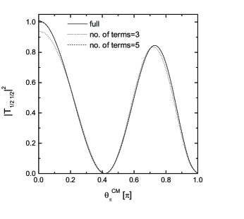
Figure 3: Angular dependence for $|T_{\frac{1}{2}\frac{1}{2}}^{++}|^{2}$ at $E_{\pi}^{LAB}=300$ MeV. Solid line is the full calculation, dashed and dotted are the resumming of partial terms.

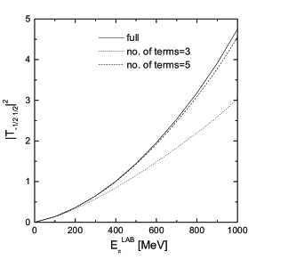
Figure 4: Energy dependence for $|T_{-\frac{1}{2}\frac{1}{2}}^{++}|^{2}$ at $\theta_{\pi}^{CM}=\pi$. The lines are defined the same as in Fig.3

In order to compare the computational efficiency of the two methods, we compare the number of partial waves needed to achieve convergence in the PWD method with the number of Gauss points for the polar-angle integration which appear in the “w/o PWD” method.

The figures show that the effect of truncations of the partial-wave series increases with the angle (Fig. 3) the energy of the incoming $\pi$ (Fig. 4). In our particular case of one-nucleon exchange computing $5$ or more partial wave amplitudes is sufficient to reproduce the full result to a 1 per cent accuracy in a broad energy domain. Thus, in this case, the efficiency of the two methods is comparable since we need 5 multipoles versus 8 Gauss points of the polar-angle integration.

It is important to emphasize that the ability to do the azimuthal-angle integration analytically is necessary to achieve comparable efficiency. We have checked that it usually takes at least 16 Gaussian points for the azimuthal integration which slows down the calculation by more than an order of magnitude.

V Extension to pion photoproduction

Our procedure for performing the analytic $\varphi$-integration is applicable in the photo- or electro-meson production to first order in the electromagnetic coupling. Here we describe the extension to the case of $\pi$ photoproduction within a simple final-state-interaction model Pas98 ; PaT03 . The model begins with the following coupled channel equation:

$$\left(\begin{array}[]{cc}T_{\pi\pi}&T_{\pi\gamma}\\ T_{\gamma\pi}&T_{\gamma\gamma}\end{array}\right)=\left(\begin{array}[]{cc}V_{\pi\pi}&V_{\pi\gamma}\\ V_{\gamma\pi}&V_{\gamma\gamma}\end{array}\right)+\left(\begin{array}[]{cc}V_{\pi\pi}&V_{\pi\gamma}\\ V_{\gamma\pi}&V_{\gamma\gamma}\end{array}\right)\left(\begin{array}[]{cc}G_{\pi}&0\\ 0&G_{\gamma}\end{array}\right)\left(\begin{array}[]{cc}T_{\pi\pi}&T_{\pi\gamma}\\ T_{\gamma\pi}&T_{\gamma\gamma}\end{array}\right)$$ (30)

where $T$ and $V$ are the amplitudes and driving potentials of the $\pi$N scattering $(\pi\pi)$, pion photo-production $(\gamma\pi)$, absorption $(\pi\gamma)$, and the nucleon Compton effect $(\gamma\gamma)$, respectively. The above equations are solved up to first order in the electromagnetic coupling $e$, hence preserving two body unitarity to this order only.

In solving the photoproduction scattering equation we calculate first $V_{\pi\pi}$ as described for $\pi$N scattering and we then iterate in the following manner:

$$T_{\pi\gamma}=V_{\pi\gamma}+V_{\pi\pi}G_{\pi}V_{\pi\gamma}+V_{\pi\pi}G_{\pi}V_{\pi\pi}G_{\pi}V_{\pi\gamma}+\ldots,$$ (31)

where we used $T_{\pi\gamma}=T_{\gamma\pi}$ from time-reversal invariance.

This solution procedure is obviously suitable for our case since the half-shell $V_{\pi\gamma}$ has a simple azimuthal angle dependence similar to the case of $V_{\pi\pi}$ (see Eq. (43)). The reduced kernel (see Eq. (47)) has two terms rather than the one term in the $\pi$N case due to the ”complication” of having to couple a spin 1 photon to spin 1/2 as opposed to coupling a spin 0 meson to spin 1/2. For example, if one considers the nucleon u-channel exchange (compare to the $\pi$N case in Eq. (B)) the half-shell photoproduction potential can be written as:

$$V_{\lambda^{\prime}\lambda\sigma}^{\rho^{\prime}\rho}(q^{\prime},q)={}_{1}V_{\lambda^{\prime}\lambda\sigma}^{\rho^{\prime}\rho}(q^{\prime}_{0},|{\bf q^{\prime}},q_{0},|{\bf q}|,\theta^{\prime})e^{-i(\lambda^{\prime}-\lambda-\sigma)\phi^{\prime}}+{}_{2}V_{\lambda^{\prime}\lambda\sigma}^{\rho^{\prime}\rho}(q^{\prime}_{0},|{\bf q^{\prime}},q_{0},|{\bf q}|,\theta^{\prime})\,e^{-i(\lambda^{\prime}+\lambda)\phi^{\prime}}$$ (32)

where $\sigma=\pm 1$ represents the helicity of the incoming photon.

One sees that when Eq. (32) is iterated in Eq. (31) two de-coupled scattering equations are obtained (each corresponding to ${}_{1}V$ or ${}_{2}V$). For each of these equations, one can show that the corresponding $\varphi^{\prime}$ dependence re-appears after doing the $\varphi^{\prime\prime}$ integration and therefore once again we can perform the azimuthal-angle integration analytically. As in the $\pi$N case, the resulting ”reduced” kernels obey 2-D integral equations.

As a check of our procedures we calculated the $u$-channel contribution to pion photoproduction using the analytic azimuthal-angle integration along with 2-D numerical integration and compared to the results of Refs. Pas98 ; PaT03 obtained using the multipole expansion. At $E_{\gamma}$ of $300$ MeV with five multipoles we found agreement to better than 1% over a wide angular range.

VI Conclusion

In recent years Glöckle and collaborators Glo88 ; Elster introduced a method which greatly simplifies the numerical integration of two-body scattering equations without performing the partial-wave expansion. The method exploits a certain azimuthal symmetry of the potential thus allowing exact integration of the azimuthal dependence. In this paper we have established general form of the azimuthal-dependence of the kernel which allows for this procedure to go through. We have argued that these conditions is in general applicable to any system of spin- 0 and/or spin- $\frac{1}{2}$ particles

We have applied this method to the case of $\pi$N system and . With some extra effort it can be applied to higher spin systems, however the procedure becomed increasingly complex with the increase of the spin of the involved particles. We have successfully applied the method to pion photo- and electro-production from the nucleon, however only to the leading order in electromagnetic coupling.

Even though we have used the Salpeter equation for or numerical exercises, the method can of course be applied to the full 4-D Bethe-Salpeter equation, which for the $\pi N$ system has so far been solved in partial waves only NiT68 ; Lah99 . Performing the azimuthal-angle integration analytically greatly facilitates finding the full solution and makes the numerical feasibility of this approach comparable to finging the solution using the partial-wave expansion.

Appendix A Helicity spinors

We define the four-component nucleon helicity spinors as follows:

$$u_{\lambda}(E_{p},{\bf p})=\frac{1}{\sqrt{2E_{p}}}\left(\begin{array}[]{c}\sqrt{E_{p}+m_{N}}\\ 2\lambda\sqrt{E_{p}-m_{N}}\end{array}\right)\otimes\chi_{\lambda}(\theta,\varphi)$$ (33)

where $\lambda=\pm 1/2$ is the helicity, $E_{p}=\sqrt{|{\bf p}|^{2}+m_{N}^{2}}$ is the energy, $\theta$ and $\varphi$ are the spherical angles of the 3-momentum ${\bf p}$, and $\chi_{\lambda}$ is the two-component Pauli spinor. The positive- and negative-energy nucleon spinors in the convention of Kubis Kub72 are defined as follows:

$$u_{\lambda}^{(\pm)}({\bf p})=u_{\lambda}(\pm E_{p},{\bf p}),$$ (34)

They satisfy the following orthogonality and completeness conditions:

$$u_{\lambda}^{\dagger(\rho)}({\bf p})\,u_{\lambda^{\prime}}^{(\rho^{\prime})}({\bf p})=\delta_{\rho\rho^{\prime}}\delta_{\lambda\lambda^{\prime}},$$ (35)

$$\sum_{\rho,\,\lambda}u_{\lambda}^{(\rho)}({\bf p})\,u_{\lambda}^{\dagger(\rho)}({\bf p})=1.$$ (36)

The Pauli spinors along the $z$-axis are given by

$$\chi_{1/2}(0)=\left(\begin{array}[]{c}1\\ 0\end{array}\right),\,\,\,\chi_{-1/2}(0)=\left(\begin{array}[]{c}0\\ 1\end{array}\right),$$

while along an arbitrary direction $\theta,\,\varphi$ they can be obtained using the Wigner rotation functions:

$$\chi_{\lambda}(\theta,\varphi)=\sum\nolimits_{\lambda^{\prime}}d^{1/2}_{\lambda\lambda^{\prime}}(\theta)\,e^{i(\lambda-\lambda^{\prime})\varphi}\,\chi_{\lambda^{\prime}}(0),$$

or, explicitly,

$$\chi_{1/2}(\theta,\varphi)=\left(\begin{array}[]{c}\cos(\theta/2)\\ e^{i\varphi}\sin(\theta/2)\end{array}\right),\,\,\,\chi_{-1/2}(\theta,\varphi)=\left(\begin{array}[]{c}-e^{-i\varphi}\sin(\theta/2)\\ \cos(\theta/2)\end{array}\right).$$

Appendix B Azimuthal dependence of one nucleon exchange

As an example, we consider the $u$-channel nucleon exchange potential given by the graph in Fig. 2 and the following expression,

$$V(q^{\prime},q;P)=\frac{g_{\pi NN}^{2}}{4m_{N}^{2}}\gamma\cdot(\beta P-q^{\prime})\gamma^{5}\frac{(\alpha-\beta)\gamma\cdot P+\gamma\cdot(q+q^{\prime})+m_{N}}{[(\alpha-\beta)P+q+q^{\prime}]^{2}-m_{N}^{2}+i\varepsilon}\gamma^{5}\gamma\cdot(\beta P-q)],$$ (37)

where $\alpha$ and $\beta$ are defined in Eq. (III). For simplicity we choose the CM frame, where the potential in the helicity basis takes the form:

$$V^{\rho^{\prime}\rho^{\prime\prime}}_{\lambda^{\prime}\lambda^{\prime\prime}}(q^{\prime},q^{\prime\prime})=\frac{g_{\pi NN}^{2}}{16\pi m_{N}^{2}}\frac{1}{u-m_{N}^{2}}\times$$

$$\times\bar{u}_{\rho^{\prime}}^{\lambda^{\prime}}({\bf q^{\prime\prime}})[M^{\rho^{\prime}\rho^{\prime\prime}}_{1}{\bf 1}+M^{\rho^{\prime}\rho^{\prime\prime}}_{2}\gamma^{0}]u_{\rho^{\prime\prime}}^{\lambda^{\prime\prime}}({\bf q^{\prime\prime}})$$ (38)

with

$$M_{1}^{\rho^{\prime}\rho^{\prime\prime}}(p^{\prime},p^{\prime\prime})=m_{N}[2\sqrt{s}(p^{\prime}_{0}+p^{\prime\prime}_{0})-s-2p^{\prime}\cdotp p^{\prime\prime}$$

$$+p^{\prime 2}+p^{\prime\prime 2}+m_{N}^{2}+(p^{\prime}_{0}-\rho^{\prime}E_{p^{\prime}})(p^{\prime\prime}_{0}-\rho^{\prime\prime}E_{p^{\prime\prime}})$$

$$-\sqrt{s}(p^{\prime}_{0}-\rho^{\prime}E_{p^{\prime}}+p^{\prime\prime}_{0}-\rho^{\prime\prime}E_{p^{\prime\prime}})]$$ (39)

$$M_{2}^{\rho^{\prime}\rho^{\prime\prime}}(p^{\prime},p^{\prime\prime})=\sqrt{s}[2\sqrt{s}(p^{\prime}_{0}+p^{\prime\prime}_{0})-s-2p^{\prime}\cdotp p^{\prime\prime}$$

$$-p^{\prime 2}-p^{\prime\prime 2}-3m_{N}^{2}-(p^{\prime}_{0}-\rho^{\prime}E_{p^{\prime}})(p^{\prime\prime}_{0}-\rho^{\prime\prime}E_{p^{\prime\prime}})]$$

$$+(p^{\prime 2}+m_{N}^{2})(p^{\prime\prime}_{0}-\rho^{\prime\prime}E_{p^{\prime\prime}})$$

$$+(p^{\prime\prime 2}+m_{N}^{2})(p^{\prime}_{0}-\rho^{\prime}E_{p^{\prime}}).$$ (40)

The azimuthal dependence $\phi^{\prime\prime}$ arises from Dirac spinors and from various scalar products involving the the four vector $q^{\prime\prime}$. Choosing the vector part of the total momentum $P$ to be along the $z$-axis (or to be zero in the CM frame) allows the $\phi^{\prime\prime}$ dependence, for the fully off-shell potential, to be displayed in the form:

$$V^{\rho^{\prime}\rho^{\prime\prime}}_{\lambda^{\prime}\lambda^{\prime\prime}}(q^{\prime},q^{\prime\prime})=\frac{g_{\pi NN}^{2}}{16\pi m_{N}^{2}}N_{q^{\prime}q^{\prime\prime}}{\Omega}_{\lambda^{\prime}\lambda^{\prime\prime}}(\theta^{\prime},\theta^{\prime\prime},\phi^{\prime},\phi^{\prime\prime})$$

$$\sum_{n=0}^{N}\frac{{\cal R}^{\rho^{\prime}\rho^{\prime\prime}}_{\lambda^{\prime}\lambda^{\prime\prime},n}(q^{\prime}_{0},|{\bf q^{\prime}}|,q^{\prime\prime}_{0},|{\bf q^{\prime\prime}}|,\theta^{\prime},\theta^{\prime\prime})cos^{n}(\phi^{\prime\prime}-\phi^{\prime})}{d_{1}(q^{\prime}_{0},|{\bf q^{\prime}}|,q^{\prime\prime}_{0},|{\bf q^{\prime\prime}}|,\theta^{\prime},\theta^{\prime\prime})+d_{2}(q^{\prime}_{0},|{\bf q^{\prime}}|,q^{\prime\prime}_{0},|{\bf q^{\prime\prime}}|,\theta^{\prime},\theta^{\prime\prime})\cos(\phi^{\prime\prime}-\phi^{\prime})},$$ (41)

where ${\cal R}^{\rho^{\prime}\rho^{\prime\prime}}_{\lambda^{\prime}\lambda^{\prime\prime},n}$, $N_{p^{\prime}p^{\prime\prime}}$, and $d_{i}$ are factors which depend on the type of the diagram and of the exchanged particle, but are independent of the azimuthal angle. The quantities,

$$\Omega_{\lambda^{\prime}\lambda^{\prime\prime}}=e^{-i\lambda^{\prime}\phi^{\prime}}\sum_{m=-1/2}^{1/2}d_{\lambda^{\prime}m}^{1/2}(\theta^{\prime})d_{\lambda^{\prime\prime}m}^{1/2}(\theta^{\prime\prime})e^{im(\phi^{\prime}-\phi^{\prime\prime})}e^{i\lambda^{\prime\prime}\phi^{\prime\prime}},$$

$$N_{q^{\prime}q^{\prime\prime}}=\sqrt{(E_{q^{\prime}}+m_{N})(E_{q^{\prime\prime}}+m_{N})/4E_{q^{\prime}}E_{q^{\prime\prime}}}$$

are factors which result from the helicity spinors. In Eq. (B) we have employed the usual trigonometric relation between two arbitrary directions defined by ${\bf q^{\prime\prime}}$ and ${\bf q^{\prime}}$:

$$\cos\Theta_{{\bf q^{\prime\prime}}{\bf q^{\prime}}}=\cos\theta^{\prime\prime}\cos\theta^{\prime}+\sin\theta^{\prime\prime}\sin\theta^{\prime}\cos(\phi^{\prime\prime}-\phi^{\prime}).$$ (42)

It is easy to see that the fully off-shell potential in Eq. (B) has the azimuthal dependence of Eq. (3). Furthermore, in iterating Eq. (14) the quantization axis is defined by the on-shell relative momentum ${\bf q}$ (i.e. $\theta=0$), hence Eq. (42) reduces to $\cos\Theta_{{\bf q^{\prime}},{\bf q}}=\cos\theta^{\prime}$, therefore the half-off-shell potential reduces to:

$$V_{\lambda^{\prime}\lambda}^{\rho^{\prime}\rho}(q^{\prime},q)=v_{\lambda^{\prime}\lambda}^{\rho^{\prime}\rho}({q_{0}^{\prime},|\bf q^{\prime}}|,q_{0},|{\bf q}|,\theta^{\prime})e^{-i(\lambda^{\prime}-\lambda)\phi^{\prime}}$$ (43)

which if of the form of the result in Eq. (4). Therefore, the azimuthal angle dependence can be removed from the Bethe-Salpeter equation for this case. We achieved this result by explicitly displaying the azimuthal angle dependence and align ${\bf P}$ with the z-axis so that only $\gamma^{3}$ and $\gamma^{0}$ appear in $V_{\lambda^{\prime}\lambda}^{\rho^{\prime}\rho}$. The presence of $\gamma^{1}$ or $\gamma^{2}$ would introduce additional azimuthal angle dependence in the spinor matrix elements and make the algebra much more complicated.

For the $u$-channel nucleon exchange the coefficients $d_{i}$ are:

$$d_{1}(p^{\prime},p^{\prime\prime})=p^{\prime 2}+p^{\prime\prime 2}+s-2\sqrt{s}(p^{\prime}_{0}+p^{\prime\prime}_{0})+2p^{\prime}_{0}p^{\prime\prime}_{0}$$

$$-2{\bf|p^{\prime}|}{\bf|p^{\prime\prime}|}\cos\theta^{\prime}\cos\theta^{\prime\prime}-m_{N}^{2}$$ (44)

$$d_{2}(p^{\prime},p^{\prime\prime})=-2{\bf|p^{\prime}|}{\bf|p^{\prime\prime}|}\sin\theta^{\prime}\sin\theta^{\prime\prime}$$ (45)

From these relations one can exactly identify the angular dependence of potential given in Eq. (37) in the 4-product,

$$p^{\prime}\cdotp p^{\prime\prime}=p^{\prime}_{0}p^{\prime\prime}_{0}-{\bf p^{\prime}}\cdot{\bf p^{\prime\prime}}$$

$$=p^{\prime}_{0}p^{\prime\prime}_{0}-{\bf|p^{\prime}|}{\bf|p^{\prime\prime}|}\cos\theta^{\prime}\cos\theta^{\prime\prime}$$

$$-{\bf|p^{\prime}|}{\bf|p^{\prime\prime}|}\sin\theta^{\prime}\sin\theta^{\prime\prime}\cos(\phi^{\prime}-\phi^{\prime\prime}).$$ (46)

The relative momenta $q^{\prime}$ and $q^{\prime\prime}$, defined in SECTION II, are to be introduced in Eq. (B) - Eq. (B) by $p^{\prime}=\alpha P+q^{\prime}$ and $p^{\prime\prime}=\alpha P+q^{\prime\prime}$

where

$$\bar{v}_{\lambda^{\prime\prime}\lambda^{\prime},\lambda}^{\rho^{\prime\prime}\rho^{\prime}}(|{\bf q^{\prime}}|,|{\bf q^{\prime\prime}}|,\theta^{\prime\prime},\theta^{\prime})=\sum_{m=-1/2}^{1/2}\sum_{n=0}^{N}{\cal R}_{\lambda^{\prime}\lambda^{\prime\prime},n}^{\rho^{\prime}\rho^{\prime\prime}}d_{\lambda^{\prime}m}^{1/2}(\theta^{\prime})d_{\lambda^{\prime\prime}m}^{1/2}(\theta^{\prime\prime})\int_{0}^{2\pi}\frac{dxcos^{n}x}{d_{1}+d_{2}\cos x}e^{i(\lambda-m)x}.$$ (47)

After applying standard trigonometric manipulations:

$$\cos^{2n-1}\theta=\frac{1}{2^{2n-2}}\left[\cos(2n-1)\theta+\left(\begin{array}[]{c}2n-1\\ 1\end{array}\right)\cos(2n-3)\theta+...+\left(\begin{array}[]{c}2n-1\\ n-1\end{array}\right)\cos\theta\right],$$

and

$$\cos^{2n}\theta=\frac{1}{2^{2n}}\left(\begin{array}[]{c}2n\\ n\end{array}\right)+\frac{1}{2^{2n-1}}\left[\cos 2n\theta+\left(\begin{array}[]{c}2n\\ 1\end{array}\right)\cos(2n-2)\theta+...+\left(\begin{array}[]{c}2n\\ n-1\end{array}\right)\cos 2\theta\right].$$

the integral over the azimuthal angle of the intermediate momentum in Eq. (47) can be reduced to integrals of the following type:

$$I_{m,n}=\int_{0}^{2\pi}\frac{d\phi\cos(m\phi)e^{in\phi}}{1+a\cos\phi}=\int_{0}^{2\pi}\frac{d\phi\cos(m\phi)\cos(n\phi)}{1+a\cos\phi}.$$ (48)

For values $|a|<1$, this definite integral can be evaluated analytically to obtain:

$$I_{m,n}=\frac{\pi}{b}\left[\left(\frac{b-1}{a}\right)^{m+n}+\left(\frac{b-1}{a}\right)^{|m-n|}\right]$$ (49)

where $b=\sqrt{1-a^{2}}$.

The results given above in Eq. (47) work for all standard particle exchanges in the s, t, or u channels. Furthermore, it should be noted that additional azimuthal angle dependences introduced by various form factors can easily be handled by simple algebraic methods. The maximum power of $cosx$ needed for a particular diagram may increase (for example, N=2 for u-channel $\Delta$ exchange). In addition, $\bar{v}$ will, in general, contain a sum of various terms corresponding to each diagram included. However, all of these terms can be evaluated using Eq. (49). In addition as noted earlier, this procedure is not at all affected by the equal time approximation and can be applied in the same manner to the full 4-D Bethe Salpeter equation.

References

• (1) J. Holz and W. Glöckle, Phys. Rev. C 37, 1386 (1988); J. Comp. Phys. 76, 131 (1988).
• (2) C. Elster, J. H. Thomas and W. Glöckle, Few Body Syst.  24, 55 (1998); W. Schadow, C. Elster and W. Glockle, Few Body Syst.  28, 15 (2000); I. Fachruddin, Ch. Elster, and W. Glockle, Phys. Rev. C62, 044002
• (3) N. K. Devine and S. J. Wallace, Phys. Rev. C 48, R973 (1993); N. K. Devine, PhD Thesis (University of Maryland, 1992).
• (4) G. Ramalho, A. Arriaga and M. T. Pena, Nucl. Phys. A 689, 511 (2001).
• (5) V. Pascalutsa and J. A. Tjon, Nucl. Phys. A 631, 534c (1998); Phys. Lett. B 435, 245 (1998).
• (6) V. Pascalutsa, PhD Thesis (University of Utrecht, 1998) [Published in: Hadronic J. Suppl.  16, 1 (2001)].
• (7) V. Pascalutsa and J. A. Tjon, Phys. Rev. C 61, 054003 (2000); ibid. 60, 034005 (1999).
• (8) M. Jacob and G.C. Wick, Ann. Phys. 7, 404 (1959).
• (9) J.J. Kubis, Phys. Rev. D 6, 547 (1972).
• (10) V. Pascalutsa and J. A. Tjon, in preparation.
• (11) H.M. Nieland and J.A. Tjon, Phys. Lett. 27B, 309 (1968).
• (12) A. D. Lahiff and I. R. Afnan, Few Body Syst. Suppl.  10, 147 (1999); Phys. Rev. C 60, 024608 (1999).