Abstract

The hadronic equation of state for a neutron star is discussed with a particular emphasis on the symmetry energy. The results of several microscopic approaches are compared and also a new calculation in terms of the self-consistent Green function method is presented. In addition possible constraints on the symmetry energy coming from empirical information on the neutron skin of finite nuclei are considered.

[]Nuclear equation of state and the structure of neutron stars

1 Introduction

In describing properties of neutron stars the equation of state (EoS) plays a crucial role as an input. During this workshop the effects of QCD degrees of freedom which become important at higher densities have been discussed in great detail. However, a quantitative understanding of the EoS also at lower densities is a prerequisite for the description of neutron stars properties. Conventional nuclear physics methods (i.e., in terms of hadronic degrees of freedom) are still being improved both conceptually as well as numerically, but all microscopic many-body approaches do require some sort of approximation scheme.

The aim of this contribution is to review the present understanding of the hadronic EoS, and the nuclear symmetry energy (SE) in particular. In the past the latter quantity has been computed mostly in terms of the Brueckner-Hartree-Fock (BHF) approach. In order to get an idea about the accuracy of the BHF result we present a recent calculation [1] in terms of the self-consistent Green function method, that can be considered as a generalization of the BHF approach. The results are compared with those from various many-body approaches, such as variational and relativistic mean field approaches. In view of the large spread in the theoretical predictions we also examine possible constraints on the nuclear SE that may be obtained from information from finite nuclei (such the neutron skin).

2 Equation of state and symmetry energy

The central quantity which determines neutron star properties is the EoS, at $T=0$ specified by the energy density $\epsilon(\rho).$ For densities above, say, $\rho=0.1$ fm^-3 one assumes a charge neutral uniform matter consisting of protons, neutrons, electrons and muons; the conditions imposed are charge neutrality, $\rho_{p}=\rho_{e}+\rho_{\mu},$ and beta equilibrium, $\mu_{n}=\mu_{p}+\mu_{e}$ with $\mu_{e}=\mu_{\mu}.$
Given the energy density $\epsilon=\epsilon_{N}+\epsilon_{e}+\epsilon_{\mu}$ the total pressure, $P=P_{N}+P_{e}+P_{\mu},$ is obtained as $P=P(\epsilon/c^{2})=\sum\rho_{i}\mu_{i}-\epsilon,$ with the chemical potentials given by $\mu_{i}=\frac{\partial\epsilon}{\partial\rho_{i}}$.

To illustrate the present status of the situation in Fig. 1 a compilation made by the Stony Brook group [2] of the relation between the pressure and density for a wide variety of EoSs (but still a tiny fraction of all available calculations) is shown.

Figure 1: Pressure versus density for a variety of EoS; taken from [2] where explanation of symbols is given.

This figure shows that there is an appreciable spreading in the calculations of the pressure. Qualitatively one can distinguish three different classes. First the EoSs that correspond to self-bound systems (such as “strange quark matter”) have the property that the pressure does not vanish at zero density. Then there are two globally parallel bands. It appears that most conventional non-relativistic approaches fall in the lower (softer) band and the covariant results in the upper (more rigid) band. It is worth noting that even at densities around and below saturation, $\rho_{0}\sim 0.17$ fm${}^{-3},$ the predictions vary appreciably (about a factor 4). At higher densities some models show a sudden change in the slope of the pressure. This behavior can be ascribed to the onset of new degrees of freedom, e.g., the appearance of hyperons, kaons and/or quarks which lead to a softening.

It is well known that at lower densities the properties of the EoS are primarily determined by the SE [2]. The latter is defined in terms of a Taylor series expansion of the energy per particle for nuclear matter in terms of the asymmetry parameter $\alpha=(N-Z)/A$ (or equivalently the proton fraction $x=Z/A$),

$$E(\rho,\alpha)=E(\rho,0)+S_{2}(\rho)\alpha^{2}+S_{4}(\rho)\alpha^{4}+\ldots,$$ (1)

where $S_{2}$ is the quadratic SE. It has been shown [3, 4] that the deviation from the parabolic law in Eq. (1), i.e., the term corresponding to $S_{4},$ is quite small.

Near the saturation density $\rho_{0}$ the quadratic SE is expanded as

$$S_{2}(\rho)=\frac{1}{2}\frac{\partial^{2}E(\rho,\alpha)}{\partial\alpha^{2}}|_{\alpha=0}=a_{4}+\frac{p_{0}}{\rho_{0}^{2}}(\rho-\rho_{0})+\frac{\Delta K}{18\rho_{0}^{2}}(\rho-\rho_{0})^{2}+\ldots.$$ (2)

The quantity $a_{4}$ corresponds to the SE at equilibrium density and the slope parameter $p_{0}$ governs the density dependence.

As a result the pressure can be written as

$$P(\rho,x)=\rho^{2}\frac{\partial E(\rho,x)}{\partial\rho}=\rho^{2}[E^{\prime}(\rho,1/2)+S_{2}^{\prime}(\rho)(1-2x)^{2}+\ldots].$$ (3)

By using beta equilibrium in a neutron star, $\mu_{e}=\mu_{n}-\mu_{p}=-\frac{\partial E(\rho,x)}{\partial x}\sim S_{2}(\rho)(1-2x),$ and the result for the electron chemical potential, $\mu_{e}=3/4\hbar cx(3\pi^{2}\rho x)^{1/3},$ one finds the proton fraction at saturation density, to be quite small, $x_{0}\sim 0.04.$ Hence the pressure at saturation density can in good approximation be expressed in terms of (the density dependence of) the SE

$$P(\rho_{0})=\rho_{0}(1-2x_{0})(\rho_{0}S_{2}^{\prime}(\rho_{0})(1-2x_{0})+S_{2}(\rho_{0})x_{0})\sim\rho^{2}_{0}S_{2}^{\prime}(\rho_{0}).$$ (4)

3 How well do we know the symmetry energy?

In the following the present status of calculations of the SE is reviewed; first the ones in which a microscopic nucleon-nucleon (NN) interaction is used, followed by the phenomenological mean field approaches. In section 4 we discuss possible constraints that can be obtained from empirical information.

3.1 The SE in the BHF scheme

In the Brueckner-Hartree-Fock (BHF) approximation, the Brueckner-Bethe-Goldstone (BBG) hole-line expansion is truncated at the two-hole-line level [5]. The short-range NN repulsion is treated by a resummation of the particle-particle ladder diagrams into an effective interaction or $G$-matrix. Self-consistency is required at the level of the BHF single-particle spectrum $\epsilon^{BHF}(k)$,

$$\epsilon^{BHF}(k)=\frac{k^{2}}{2m}+\sum_{k^{\prime}<k_{F}}\mbox{Re}<kk^{\prime}|G(\omega=\epsilon^{BHF}(k)+\epsilon^{BHF}(k^{\prime}))|kk^{\prime}>.$$ (5)

In the standard choice BHF the self-consistency requirement (5) is restricted to hole states ($k<k_{F},$ the Fermi momentum) only, while the free spectrum is kept for particle states $k>k_{F}$. The resulting gap in the s.p. spectrum at $k=k_{F}$ is avoided in the continuous-choice BHF (ccBHF), where Eq. (5) is used for both hole and particle states. The continuous choice for the s.p. spectrum is closer in spirit to many-body Green’s function perturbation theory (see below). Moreover, recent results indicate [6, 7] that the contribution of higher-order terms in the hole-line expansion is considerably smaller if the continuous choice is used.

Although the BHF approach has several shortcomings it provides a numerically simple and convenient scheme to provide insight in some aspects of the symmetry energy.

Decomposition of SE

Some insight into the microscopic origin of the SE can be obtained by examining the separate contributions to the kinetic and potential energy [3].

The results of a ccBHF calculation [1] with the Reid93 interaction, including partial waves with $J<4$ in the calculation of the G-matrix are presented in Fig. 3.1, where the SE is decomposed into various contributions shown as a function of the density $\rho$.

The SE $S_{2}$ (full line) and the contributions to $S_{2}$ from the kinetic (dash-dotted line) and potential energy (dashed line), calculated within a ccBHF scheme and using the Reid93 interaction. Also shown (dotted lines) are the $T=0$ and $T=1$ components of the potential energy contribution.

The kinetic energy contribution, $S_{\rm kin},$ to the SE in BHF is given by the free Fermi-gas expression (it differs from the standard one, which is based upon the derivative rather than the finite difference)

$$S_{\rm kin}=E_{\rm kin,PNM}-E_{\rm kin,SNM}=\frac{3}{10m}(3\pi^{2})^{\frac{2}{3}}\rho^{\frac{2}{3}}\left(1-{2^{-\frac{2}{3}}}\right),$$ (6)

and it determines to a large extent the density dependence of the SE. In Fig. 3.1 we also show the symmetry potential $S_{\rm pot}=S_{2}-S_{\rm kin}$, which is much flatter, and the contributions to $S_{\rm pot}$ from both the isoscalar ($T=0$) and isovector ($T=1$) components of the interaction. Over the considered density range $S_{\rm pot}$ is dominated by the positive $T=0$ part. The $T=0$ partial waves, containing the tensor force in the ${}^{3}S_{1}$-${}^{3}D_{1}$ channel which gives a major contribution to the potential energy in SNM, do not contribute to the PNM energy. The $T=0$ contribution peaks at $\rho\approx 0.3$ fm^-3. The decrease of this contribution at higher densities is compensated by the increase of the $T=1$ potential energy, with as a net result a much weaker density-dependence of the total potential energy.

Dependence of the SE on NN interaction

Engvik et al. [8] have performed lowest-order BHF calculations in SNM and PNM for all “modern” potentials (CD-Bonn, Argonne v18, Reid93, Nijmegen I and II), which fit the Nijmegen NN scattering database with high accuracy. They concluded that for small and normal densities the SE is largely independent of the interaction used, e.g. at $\rho_{0}$ the value of $a_{4}$ varies around an average value of $a_{4}$=29.8 MeV by about 1 MeV. At larger densities the spread becomes larger; however, the SE keeps increasing with density, in contrast to some of the older potentials like Argonne v14 and the original Reid interaction (Reid68) for which $S(\rho)$ tends to saturate at densities larger than $\rho=0.4$ fm^-3.

3.2 Variational approach

Detailed studies for SNM and PNM using variational chain summation (VCS) techniques were performed by Wiringa et al. [9] for the Argonne Av14 NN interaction in combination with the Urbana UVIII three-nucleon interaction (3NI), and by Akmal et al. [10] for the modern Av18 NN potential in combination with the UIX-3NI.

It should be noted that the results of VCS and BHF calculations using the same NN interaction disagree in several aspects. For instance for SNM the VCS and BHF calculations saturate at different values of density [5]. As for the SE using only two-body interactions the VCS approach yields a smaller value for $a_{4}$ than BHF (see Table 1), and as a function of density in VCS the SE levels off at $\rho\sim 0.6$ fm${}^{-3},$ whereas the BHF result continues to increase. Therefore it seems natural to ask whether the inclusion of more correlations by extending the BHF method (which is basically a mean field approximation) will lead to results closer to those of VCS.

3.3 Self-consistent Green function method

As noted above BHF has several deficiencies: it does not saturate at the empirical density, and it violates the Hugenholz-van Hove theorem.

In recent years several groups have considered the replacement of the BBG hole-line expansion with self-consistent Green’s function (SCGF) theory [11, 12, 13]. In ref.[13, 14] the binding energy for SNM was calculated within the SCGF framework using the Reid93 potential. In ref.[1] we have extended these calculations to PNM and considered the corresponding SE.

The SCGF approach differs in two important ways from the BHF scheme. Firstly, within SCGF particles and holes are treated on an equal footing, whereas in BHF only intermediate particle $(k>k_{F})$ states are included in the ladder diagrams. This aspect ensures thermodynamic consistency, e.g. the Fermi energy or chemical potential of the nucleons equals the binding energy at saturation (i.e. it fulfills the Hugenholz-van Hove theorem). In the low-density limit BHF and SCGF coincide. As the density increases the phase space for hole-hole propagation is no longer negligible, and this leads to an important repulsive effect on the total energy. Second, the SCGF generates realistic spectral functions, which are used to evaluate the effective interaction and the corresponding nucleon self-energy. The spectral functions exhibits a depletion of the quasi-particle peak and the appearance of single-particle strength at large values of energy and momentum, in agreement with experimental information from $(e,e^{\prime}p)$ reactions. This is in contrast with the BHF approach where all s.p. strength is concentrated at the BHF-energy as determined from Eq. (5).

In the SCGF approach the particle states ($k>k_{F}$), which are absent in the BHF energy sum rule do contribute according to the energy sum rule ($d=1(2)$ for PNM(SNM))

$$\frac{E}{A}=\frac{d}{\rho}\int\frac{d^{3}k}{(2\pi)^{3}}\int_{-\infty}^{\varepsilon_{F}}d\omega\ \left(\frac{k^{2}}{2m}+\omega\right)S_{h}(k,\omega),$$ (7)

expressed in terms of the nucleon spectral function $S_{h}(k,\omega)$.

To illustrate the difference between the ccBHF and SCGF approaches the results for both SNM and PNM are compared in the left and central panels of Fig. 2 for the Reid93 interaction. One sees that the inclusion of high-momentum nucleons leads roughly to a doubling of the kinetic and potential energy in SNM, as compared to BHF. The net effect for the total energy of SNM is a repulsion, increasing with density [13]. This leads to a stiffer equation of state, and a shift of the SNM saturation density towards lower densities. The above effects which are dominated by the tensor force (the isoscalar ${}^{3}S_{1}$-${}^{3}D_{1}$ partial wave) are much smaller in PNM.

The corresponding SE, shown in the right panel of Fig. 2, is dominated by the shift in the total energy for SNM, and lies below the ccBHF symmetry energy in the entire density-range. At $\rho_{0}=0.16$ fm^-3 the parameter $a_{4}$ is reduced from 28.9 MeV to 24.9 MeV, while the slope $p_{0}$ remains almost the same (2.0 MeVfm^-3 compared to 1.9 MeVfm^-3 in BHF).

Figure 2: The energy per particle for symmetric nuclear matter (left panel) and pure neutron matter (central panel) for the Reid93 interaction. The dashed line refers to a ccBHF calculation, the full line to a SCGF calculation. The right panel displays the SE in these two approaches.

3.4 Three-body force in microscopic approaches

As noted above at higher densities the EoS is sensitive to 3NF contributions. Whereas the 3NF for low densities seems now well understood its contribution to nuclear matter densities remains unsettled. In practice in calculations of the symmetry energy in the BHF approach two types of 3NF have been used in calculations; in ref.[4] the microscopic 3NF based upon meson exchange by Grangé et al. was used, and in ref.[15] as well in most VCS calculations the Urbana interaction. The latter has in addition to an attractive microscopic two-pion exchange part a repulsive phenomenological part constructed in such a way that the empirical saturation point for SNM is reproduced. Also in practice in the BHF approach to simplify the computational efforts the 3NF is reduced to a density dependent two-body force by averaging over the position of the third particle.

In general inclusion of the 3NF stiffens the SE for $\rho>\rho_{0}.$ For example, with the Av18+UIX interaction $a_{4}$ increases from 27 to 30 MeV and $p_{0}$ from 2 to 3 MeVfm^-3 (see Table 1).

In view of the important contribution from the 3NF to the SE at higher densities there seems a clear need to get a more quantitative understanding of the repulsive part of the 3NF in PNM.

3.5 Dirac-Brueckner-Hartree-Fock

The SE has also been computed in the Dirac-Brueckner-Hartree-Fock (DBHF) approach [16, 17]. Although some of the shortcomings of BHF (mean field treatment of the Pauli operator and violation of Hugenholz-van Hove theorem) persist in the DBHF method it appears that in the latter approach one is able to reproduce the saturation properties of SNM without the inclusion of a three-body interaction. A general feature of relativistic methods is that the SE increases almost linearly with density, and more rapidly than in the non-relativistic case. This difference can be attributed to two effects. First the covariant kinetic energy which is inversely proportional to $\sqrt{k_{F}^{2}+m^{*2}}$ is larger because of the decreasing Dirac mass, $m^{*}$, with increasing density. Secondly the contribution from rho-exchange appears to be larger than in the non-relativistic case [16].

3.6 Relativistic mean-field approach

Relativistic mean field (RMF) models have been applied succesfully to describe properties of finite nuclei. In general ground state energies, spin-orbit splittings, etc. can be described well in terms of a few parameters ref.[18]. Recently it has lead to the suggestion that the bulk SE is strongly correlated with the neutron skin [19, 20] (see below). In essence the method is based upon the use of energy-density functional (EDF) theory.

In practice covariant approaches are formulated either in terms of a covariant lagrangian with $\sigma,\ \omega$ and $\rho$ exchange (and possibly other mesons) [18, 21], or in terms of contact interactions [20], solved as an EDF in the Hartree-Fock approximation. Sets of model parameters are determined by fitting bound state properties of nuclei. Specifically the isovector degree of freedom is governed by the exchange of isovector mesons; in case of $\rho$-meson exchange the (positive definite) contribution to the SE is given by

$$a_{4}=\frac{k^{2}_{F}}{6\sqrt{m^{*2}+k_{F}^{2}}}+\frac{g^{2}_{\rho}}{8m^{2}_{\rho}}\rho_{0},$$ (8)

and its potential energy contribution to $p_{0}$, which scales with that for $a_{4}$, is $\frac{g^{2}_{\rho}}{8m^{2}_{\rho}}$ [20]. Typical values obtained for $p_{0}$ are around 4-6 MeV fm^-3, and $a_{4}\sim$ 30-36 MeV, i.e., considerably larger than in non-relativistic approaches (a large part of the enhancement can be ascribed to the fact that the kinetic contribution is larger, because $m^{*}<m$).

Recently this approach was extended by inclusion of the isovector-scalar partner, the $\delta$-meson, of the isoscalar scalar $\sigma$-meson [22]. Unfortunately the value of the coupling for the $\delta$-meson cannot be determined well by fitting properties of stable nuclei. Also in its simplest, density independent form, the inclusion of the $\delta$-meson leads to an even larger net value for $p_{0}$. This happens because of the presence of the Lorentz factor $m^{*}/E$ in the scalar potential contribution, $\sim-\frac{g_{\delta}^{2}}{8m_{\delta}^{2}}\frac{m^{*}}{E},$ which decreases with increasing density.

3.7 Effective field theory

Recently the density dependence of the symmetry energy has been computed in chiral perturbation effective field theory, described by pions plus one cutoff parameter, $\Lambda,$ to simulate the short distance behavior [23]. The nuclear matter calculations have been performed up to three-loop order; the density dependence comes from the replacement of the free nucleon propagator by the in-medium one, specified by the Fermi momentum $k_{F}$

$$(/p+M)\left(\frac{i}{p^{2}-M^{2}+i\epsilon}-2\pi\delta(p^{2}-M^{2})\theta(p_{0})\theta(k_{F}-p)\right).$$

The resulting EoS is expressed as an expansion in powers of $k_{F}$ and the value of $\Lambda\approx 0.65$ GeV is adjusted to the empirical binding energy per nucleon. In its present form the validity of this approach is clearly confined to relatively small values of the Fermi momentum, i.e. rather low densities. Remarkably for SNM the calculation appears to be able to reproduce the microscopic EoS up to $\rho\sim 0.5$ fm^-3. As for the SE the value obtained in this approach for $a_{4}=33$ MeV is in reasonable agreement with the empirical one; however, at higher densities ($\rho>0.2$ fm^-3) a downward bending is predicted (see Fig. 3) which is not present in other approaches.

3.8 Comparison of results

To summarize the present situation in Fig. 3 the resulting density dependence of the SE for the approaches discussed above are compared (excluding the 3NF contribution). One sees that the covariant models predict a much larger increase of the SE with the density than the non-relativistic approaches. The lowest-order BHF method predicts a somewhat higher value for $a_{4}$ than both the VCS and SCGF methods, which lead to very similar results; whether that can be ascribed to a consistent treatment of correlations in these methods, or is fortuitous, is not clear.

Figure 3: Overview of several theoretical predictions for the SE: Brueckner-Hartree-Fock (continuous choice) with Reid93 potential (circles), self-consistent Green function theory with Reid93 potential (full line), variational calculation from [9] with Argonne Av14 potential (dashed line), DBHF calculation from [16] (triangles), relativistic mean-field model from [22] (squares), effective field theory from [23] (dash-dotted line).

Table 1: Results for the symmetry energy parameters $a_{4}$ (in MeV) and $p_{0}$ (in MeVfm^-3)

	BHF	BHF+3NF[5]	VCS[10]	VCS+3NF[10]	SCGF[1]	DBHF[16]	RMF[20]
$a_{4}$	28.9	30	27	30	24.9	31	30-36
$p_{0}$	1.9	2.9	2.0	3.1	2.0	3.0	4-6

Clearly at least part of the differences should be attributed to the different selection of the mesonic degrees of freedom in the various models. In the microscopic approaches the tensor force mediated by $\pi$ and $\rho$ exchange seems to play the dominant role. On the other hand in the mean field approach explicit pion exchange is usually not included and hence there the isovector effect solely comes from the shorter range $\rho$-exchange. In fact it has been argued that in contrast to isoscalar properties the long-range pion exchange should play an essential role in determining the isovector properties [20].

4 Empirical information on the SE

In view of the existing uncertainties in the calculation of the SE one may ask whether from finite nuclei one can obtain experimental constraints on the symmetry energy as a function of density. In this section some recent activities pertaining to this issue are reviewed.

4.1 Relation between SE and neutron skin

Recently in applying the non-relativistic Skyrme Hartree-Fock (SHF) model Brown [19] noted that certain combinations of parameters in the SHF are not well determined by a fit to ground state binding energies alone; as a result a wide range of predictions for the EoS for PNM can be obtained. At the same time he found a correlation between the derivative of the neutron star EoS (i.e., basically the symmetry pressure $p_{0}$) and the neutron skin in ²⁰⁸Pb.

Subsequently Furnstahl [20] in a more extensive study pointed out that within the framework of mean field models (both non-relativistic Skyrme as well as relativistic models) there exists an almost linear empirical correlation between theoretical predictions for both $a_{4}$ and its density dependence, $p_{0},$ and the neutron skin, $\Delta R=R_{n}-R_{p},$ in heavy nuclei. This is illustrated for ²⁰⁸Pb in Fig. 4 (from ref.[20]; a similar correlation is found between $\Delta R$ and $p_{0}$). Note that whereas the Skyrme results cover a wide range of $\Delta R$ values the RMF predictions in general lead to $\Delta R>0.20$ fm.

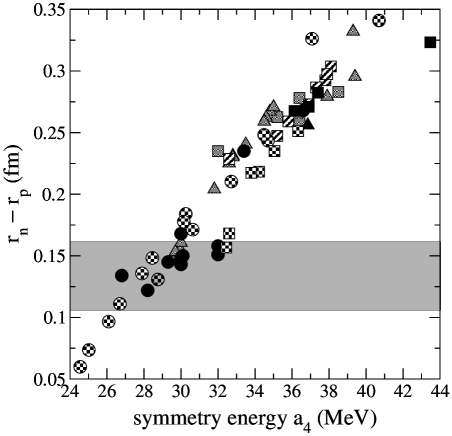
Figure 4: Neutron skin thickness versus $a_{4}$ for ²⁰⁸Pb for a variety of mean field models (from [20]). The circles correspond to results for the Skyrme force, the squares to RMF models with mesons, and the triangles to RMF with point couplings; the shaded area indicates the range of $\Delta R$ values consistent with the present empirical information for ²⁰⁸Pb.

The interpretation of the nuclear matter results in part depends on the question whether there is a surface contribution to the SE in finite nuclei. In ref.[24] it was found that for heavy nuclei the latter is of minor importance, which has also been confirmed in ref.[20].

4.2 Insight in the correlation of $\Delta R$ and $a_{4}$

The above observation suggests an intriguing relationship between a bulk property of infinite nuclear matter and a surface property of finite systems.
Here we want to point out that this correlation can be understood naturally in terms of the Landau-Migdal approach. To this end we consider a simple mean-field model (see, e.g., ref.[25]) with the Hamiltonian consisting of the single-particle mean field part $\hat{H}_{0}$ and the residual particle-hole interaction $\hat{H}_{ph}$:

$$\hat{H}=\sum\limits_{a}(T_{a}+U_{0}(x_{a})+U_{1}(x_{a})+U_{C}(x_{a}))+\hat{H}_{ph},$$ (9)

where $(x=(r,\sigma,\tau))$

$$U_{0}(x)=U_{0}(r)+U_{so}(x);\ U_{1}(x)=\frac{1}{2}S_{\rm pot}(r)\tau^{(3)};\ U_{C}(x)=\frac{1}{2}U_{C}(r)(1-\tau^{(3)}).$$

Here, the mean field potential includes the phenomenological isoscalar part $U_{0}(x)$ along with the isovector $U_{1}(x)$ and the Coulomb $U_{C}(x)$ parts calculated consistently in the Hartree approximation; $U_{0}(r)$ and $U_{so}(x)=U_{so}(r)\vec{\sigma}\cdot\vec{l}$ are the central and spin-orbit parts of the isoscalar mean field, respectively, and $S_{\rm{pot}}(r)$ is the potential part of the symmetry energy.
In the Landau-Migdal approach the effective isovector particle-hole interaction $\hat{H}_{ph}$ is given by

$$\hat{H}_{ph}=\sum\limits_{a>b}(F^{\prime}+G^{\prime}\vec{\sigma}_{a}\vec{\sigma}_{b})\vec{\tau}_{a}\vec{\tau}_{b}\delta(\vec{r}_{a}-\vec{r}_{b}),$$ (10)

where $F^{\prime}$ and $G^{\prime}$ are the phenomenological Landau-Migdal parameters.

The model Hamiltonian $\hat{H}$ in Eq.(9) preserves isospin symmetry if the condition

$$[\hat{H},\hat{T}^{(-)}]=\hat{U}^{(-)}_{C},$$ (11)

is fulfilled, where $\hat{T}^{(-)}=\sum\limits_{a}\tau_{a}^{(-)},\ \hat{U}^{(-)}_{C}=\sum\limits_{a}U_{C}(r_{a})\tau_{a}^{(-)}.$ With the use of Eqs. (9),(10) the condition eq.(11) in the random phase approximation (RPA) formalism leads to a self-consistency relation between the symmetry potential and the Landau parameter $F^{\prime}$ [26]:

$$S_{\rm{pot}}(r)=2F^{\prime}n^{(-)}(r),$$ (12)

where $n^{(-)}(r)=n^{n}(r)-n^{p}(r)$ is the neutron excess density. Thus, in this model the depth of the symmetry potential is controlled by the Landau-Migdal parameter $F^{\prime}$ (analogously to the role played by the parameter $g_{\rho}^{2}$ in relativistic mean field models).

$S_{\rm{pot}}(r)$ is obtained from Eq. (12) by an iterative procedure; the resulting dependence of $\Delta R$ on the dimensionless parameter $f^{\prime}=F^{\prime}/(300$ MeV fm³) shown in fig. 5 indeed illustrates that $\Delta R$ depends almost linearly on $f^{\prime}.$ Then with the use of the Migdal relation [27] which relates the SE and $f^{\prime},$

$$a_{4}=\frac{\epsilon_{F}}{3}(1+2f^{\prime}),$$ (13)

an almost linear correlation between the symmetry energy, $a_{4},$ and the neutron skin is found.

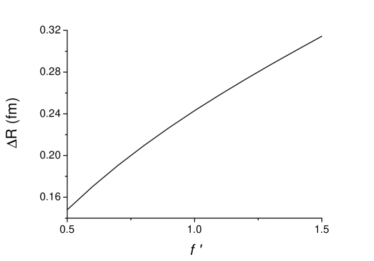
Figure 5: Neutron skin in ²⁰⁸Pb vs. the Landau-Migdal parameter $f^{\prime}$.

To get more insight in the role of $f^{\prime}$ we consider small variations $\delta F^{\prime}$. Neglecting the variation of $n^{(-)}(r)$ with respect to $\delta F^{\prime}$ one has a linear variation of the symmetry potential: $\delta S_{pot}(r)=2\delta F^{\prime}n^{(-)}(r)$. Then in first order perturbation theory, such a variation of $S_{pot}$ causes the following variation of the ground-state wave function

$$|\delta 0\rangle=\delta F^{\prime}\sum\limits_{s}\frac{\langle s|\hat{N}^{(-)}|0\rangle}{E_{0}-E_{s}}|s\rangle,$$ (14)

with $s$ labeling the eigenstates of the nuclear Hamiltonian and a single-particle operator $\hat{N}^{(-)}=\sum\limits_{a}n^{(-)}(r_{a})\tau^{(3)}_{a}$. Consequently the variation of the expectation value of the single-particle operator $\hat{V}^{(-)}=\sum\limits_{a}r^{2}_{a}\tau^{(3)}_{a}$ with $\langle 0|\hat{V}^{(-)}|0\rangle=NR^{2}_{n}-ZR^{2}_{p}$ can be written as

$$R_{p}\delta(\Delta R)=\delta F^{\prime}\frac{2}{A}\sum\limits_{s}\frac{{\rm Re}\langle 0|\hat{N}^{(-)}|s\rangle\langle s|\hat{V}^{(-)}|0\rangle}{E_{0}-E_{s}}.$$ (15)

In practice the sum in Eq. (15) is exhausted mainly by the isovector monopole resonance of which the high excitation energy (about 24 MeV in ²⁰⁸Pb) justifies the perturbative consideration. We checked that Eq. (15) is able to reproduce directly calculated $\delta(\Delta R)$ shown in fig. 5 with the accuracy of about 10%.
As for the correlation between $\Delta R$ and $p_{0}$ one would need information on the density dependence of $F^{\prime}.$ Sofar as we know it has not been extracted from data on stable nuclei. In the approximation that $F^{\prime}$ is density independent one naturally finds the $p_{0}$ is proportional to $a_{4}.$

4.3 Experimental information on $\Delta R$ for ²⁰⁸Pb

What are the experimental constraints on the neutron skin? A variety of experimental approaches have been explored in the past to obtain information on $\Delta R.$ To a certain extent all analysis contain a certain model dependence, which is difficult to estimate quantitatively. It is not our intention to present a full overview of existing methods for the special case of ²⁰⁸Pb. In particular the results obtained in the past from the analysis of elastic scattering of protons and neutrons have varied depending upon specifics of the analysis employed. At present the most accurate value for $\Delta R$ comes from a recent detailed analysis of the elastic proton scattering reaction at $E=0.5-1$ GeV [28], and of neutron and proton scattering at $E=40-100$ MeV [29]. For details we refer to these papers. Here we restrict ourselves to a discussion of the some less well known methods that have the potential to provide more accurate information on the neutron skin in the future.

Anti-protonic atoms

Recently neutron density distributions in a series of nuclei were deduced from anti-protonic atoms [30]. The basic method determines the ratio of neutron and proton distributions at large differences by means of a measurement of the annihilation products which indicates whether the antiproton was captured on a neutron or a proton. In the analysis two assumptions are made. First a best fit value for the ratio $R_{I}$ of the imaginary parts of the free space $\bar{p}p$ and $\bar{p}n$ scattering lengths equal to unity is adopted. Secondly in order to reduce the density ratio at the annihilation side to a a ratio of rms radii a two-parameter Fermi distribution is assumed. The model dependence introduced by these assumptions is difficult to judge. Since a large number of nuclei have been measured one may argue that the value of $R_{I}$ is fixed empirically.

Parity violating electron scattering

Recently it has been proposed to use the (parity violating) weak interaction to probe the neutron distribution. This is probably the least model dependent approach [31]. The weak potential between electron and a nucleus

$$\tilde{V}(r)=V(r)+\gamma_{5}A(r),$$ (16)

where the axial potential $A(r)=\frac{G_{F}}{2^{3/2}}\rho_{W}(r).$ The weak charge is mainly determined by neutrons

$$\rho_{W}(r)=(1-4\sin^{2}\theta_{W})\rho_{p}(r)-\rho_{n}(r),$$ (17)

with $\sin^{2}\theta_{W}\approx 0.23.$ In a scattering experiment using polarised electrons one can determine the cross section asymmetry [31] which comes from the interference between the $A$ and $V$ contributions. Using the measured neutron form factor at small finite value of $Q^{2}$ and the existing information on the charge distribution one can uniquely extract the neutron skin. Some slight model dependence comes from the need to assume a certain radial dependence for the neutron density, to extract $R_{n}$ from a finite $Q^{2}$ form factor.

Giant dipole resonance

Isovector giant resonances contain information about the SE through the restoring force. In particular the excitation of the isovector giant dipole resonance (GDR) with isoscalar probes has been used to extract $\Delta R/R$ [32]. In the distorted wave Born approximation optical model analysis of the cross section the neutron and proton transition densities are needed as an input. For example, in the Goldhaber-Teller picture these are expressed as

$$g_{i}(r)=-\kappa\frac{2N_{i}}{A}\frac{d\rho_{i}}{dr}$$ (18)

with $\kappa$ the oscillation amplitude and $(i=p,n)$; one assumes ground state neutron and proton distributions of the form $(x=(N-Z)/A)$

$$\rho_{i}(r)=\frac{1}{2}(1\pm x\mp\gamma x)\rho(r-c(1\pm\gamma x/3)),$$ (19)

where $\gamma$ is related to the neutron skin $\Delta R,$ $\gamma=\frac{3A}{2(N-Z)}\Delta R/R_{0}.$ Then for $N>Z$ the isovector transition density takes on the form

$$\Delta g(r)=\kappa\gamma\frac{N-Z}{A}(\frac{d\rho}{dr}+\frac{c}{3}\frac{d^{2}\rho}{dr^{2}}),$$

In practice one studies the excitation of the GDR by alpha particle scattering (isoscalar probe). By comparing the experimental cross section with the theoretical one (calculated as a function of the ratio $\Delta R/R$) the value of $\Delta R$ can be deduced [32].

It is difficult to make a quantitative estimate of the uncertainty in the result coming from the model dependence of the approach. In the analysis several assumptions must be made, such as the radial shape of the density oscillations and the actual values of the optical model parameters.

We note that also other types of isovector giant resonances have been suggested as a source of information on the neutron skin, such as the spin-dipole giant resonance [33] and the isobaric analogue state [34]. At present studies of these reactions have not led to quantitative constraints for the neutron skin of ²⁰⁸Pb.

Results for $\Delta R$

In table 2 we present a summary of some recent results on $\Delta R$ in ²⁰⁸Pb. One sees that the recent results are consistent with $\Delta R$ values in the range 0.10-0.16 fm. It appears from Fig. 4 that this range is consistent with the conventional Skyrme model approach but tends to disagree with the results of the RMF models considered in [20]. Also from the correlation plot between $\Delta R$ and $p_{0}$ shown in Fig. 11 in ref.[20] one may conclude that a small value for $p_{0}\sim 2.0$ MeVfm^-3 is favoured over the larger values from covariant models.

Table 2: Summary of recent results for $\Delta R$ in ²⁰⁸Pb

method	$\Delta R$ [fm]	error [fm]	ref
($\vec{p},p^{\prime})$ at 0.5-1.04 GeV	0.097	0.014	[28]
nucleon scattering (40-200 MeV)	0.17		[29]
anti-protonic atoms	0.15	0.02	[30]
giant dipole resonance excitation	0.19	0.09	[32]
parity violating electron scattering	planned	1%	[31]

4.4 Information on the SE from heavy-ion reactions

In principle the density dependence of the SE at higher densities (and further away from $N=Z$) can be probed by means of heavy-ion reacties using neutron rich radioactive beams. In ref.[35] possible observable effects from the isovector field are considered in terms of the RMF model. Of particular interest seems the study of the ratio of $\pi^{+}/\pi^{-}$ cross sections and its energy dependence which appears sensitive to details of the SE [36].

5 Constraints on EoS from neutron stars

Given the EoS as a function of density the mass versus radius relation of a neutron star can be obtained in the standard way with the use of the Tolman-Oppenheimer-Volkov equation. Do we need the EoS up to all densities or can we already draw some conclusions from the lower densities? In [2] it was argued that there exists a quantitative correlation between the neutron star radius and the pressure which does not depend strongly on the EoS at the highest densities. Generally speaking a stiff (soft) EoS implies a large (small) radius.

Clearly a simultaneous measurement of the radius and the mass of the same star would discriminate between various EoS. The presently available observations do not yet offer strong constraints. For example, most observed star masses fall in the range of 1.3-1.5 $M_{\odot}.$ These values seem to rule out the very soft EoSs predicted with hyperons present, which yield $M_{max}\sim 1.3M_{\odot}$ [5]. This may suggest that either the NY and YY interactions used as an input must be reexamined, or that the use of the BHF approach at high densities is not reliable.

Other constraints come from recent observations from X-ray satellites. Most robust seem the data from the low mass X-ray binary EXO 0478-676 obtained by Cottam et al. [37]. From the redshifted absorption lines from ionized Fe and O a gravitational redshift $z=0.23$ was deduced; this gives rise to a mass-to-radius relation

$$M/M_{\odot}=(1-\frac{1}{(1+z)^{2}})R/R_{g\odot}$$ (20)

with $R_{g\odot}=2.95$ km. As discussed in detail in various contributions in this workshop at present this constraint appears fully consistent not only with conventional EoSs, but also with most more exotic ones.

1

References

- [1] A.E.L. Dieperink et al., to appear in Phys. Rev. C
- [2] J.M. Lattimer and M.Prakash, Astrophys. J. 550 426 (2001)
- [3] W. Zuo, I. Bombaci and U. Lombardo, Phys.Rev.C60 024605 (1999)
- [4] W. Zuo et al. Eur. Phys. J. A14 469 (2002)
- [5] M. Baldo anf F. Burgio, Lect. Notes Phys. 578 1 (2001)
- [6] M. Baldo, G. Giansiracusa, U. Lombardo and H.Q. Song, Phys. Lett. B473, 1 (2000)
- [7] M. Baldo, A. Fiasconaro, H.Q. Song, G. Giansiracusa and U. Lombardo, Phys.Rev.C65, 017303 (2001)
- [8] L. Engvik, M. Hjorth-Jensen, R. Machleidt, H. Müther and A. Polls, Nucl.Phys.A627 85 (1997)
- [9] R.B. Wiringa, V. Fiks and A. Fabrocini, Phys.Rev.C38,1010 (1988)
- [10] A. Akmal, V.R. Pandharipande, D.G. Ravenhall, Phys.Rev.C581804(1998)
- [11] P. Bozek, Phys. Rev. C65, 054306 (2002); Eur. Phys. J. A15, 325 (2002); P. Bozek and P. Czerski, Eur. Phys. J. A11, 271 (2001)
- [12] Y. Dewulf, D. Van Neck and M. Waroquier, Phys. Lett. B510, 89 (2001)
- [13] Y. Dewulf, D. Van Neck and M. Waroquier, Phys. Rev. C65, 054316 (2002)
- [14] Y. Dewulf, W.H. Dickhoff, D. Van Neck , E.R. Stoddard and M. Waroquier, Phys. Rev. Lett. 90 152501 (2003)
- [15] M. Baldo, I Bombaci, and G.F. Burgio, Astron. and Astrophys. 328, 274 (1997)
- [16] C.-H. Lee, T.T.S. Kuo, G.Q. Li and G.E. Brown, Phys. Rev. C57 3488(1998)
- [17] K. Sumiyoshi, K. Oyamatsu, and H. Toki, Nucl.Phys. A595 327(1995)
- [18] P. Ring, Progr. Part. Nucl. Phys. 37 193 (1996), and refs therein
- [19] B.A. Brown, Phys. Rev. Lett. 85 5296 (2000)
- [20] R.J. Furnstahl, Nucl. Phys. A706 85 (2002); and nucl-th/0307111
- [21] C.J. Horowitz and J. Piekarewicz, Phys. Rev. C66 055803(2002)
- [22] B. Liu et al., Phys. Rev. C65 045201 (2002)
- [23] N. Kaiser, S. Fritsch, and W. Weise, Nucl. Phys. A697 255 (2002)
- [24] K. Oyamatsu et al., Nucl. Phys. A634 3 (19980
- [25] M.L. Gorelik, S. Shlomo and M.H. Urin, Phys. Rev. C 62, 044301 (2000).
- [26] B.L. Birbrair and V.A. Sadovnikova, Sov. J. Nucl. Phys. 20, 347 (1975); O.A. Rumyantsev and M.H. Urin, Phys. Rev. C49, 537 (1994).
- [27] A.B. Migdal, Theory of Finite Fermi Systems and Applications to Atomic Nuclei (Interscience, London, 1967)
- [28] B.C. Clark, L.J.Kerr and S. Hama, Phys. Rev. C67 054605 (2003)
- [29] S. Karataglidis, K. Amos, B.A. Brown and P.K. Deb, Phys. Rev. C65 044306 (2002)
- [30] A. Trzcinska et al., Phys. Rev. Lett. 87 082501(2001)
- [31] C. Horowitz et al., Phys. Rev. C63 025501 (2001)
- [32] A. Krasznahorkay et al., Nucl. Phys. A567 521 (1994)
- [33] A. Krasznahorkay et al., Phys. Rev. Lett. 82 3216 (1999)
- [34] N. Auerbach, J. Huefner, A.K. Kerman, C.M. Shakin, Revs. Mod. Phys. 44 48(1972)
- [35] T. Gaitanos et al., nucl-th/0309021
- [36] Bao-An Li, Phys. Rev. C67 017601 (2003) and refs. therein
- [37] J. Cottam, F. Paerels and M. Mendez, Nature 420 51 (2002)