subject

Structure studies of conventional and novel excitations to the continuum in reactions with unstable nuclei

Chapter 1 Preface

He had a weak point – this Fortunato – although in other regards he was a man to be respected and even feared. He prided himself on his connoisseurship in wine. Few Italians have the true virtuoso spirit. For the most part their enthusiasm is adopted to suit the time and opportunity to practise imposture upon the British and Austrian MILLIONAIRES. In painting and gemmary, Fortunato, like his countrymen , was a quack, but in the matter of old wines he was sincere. In this respect I did not differ from him materially; I was skilful in the Italian vintages myself, and bought largely whenever I could.
- The cask of Amontillado amontillado - Edgar Allan Poe.

1.1 Introduction and motivations

We are now living a new era of development of nuclear sciences that has expanded recently thanks to the discovery of the so-called exotic nuclei. These nuclei lie far from the stability valley, and are also named unstable nuclei in contrast to the stable ones, which nuclear scientists were used to deal with in the past. The Odyssey to reach the limits of stability, is pushing nuclear sciences to new and unexpected discoveries and to a redefinition of its scope and methods. At a variance with other revolutions happened suddenly in science, this is a quite slow and step-by-step revolution, that is both experimentally and theoretically a scientific challenge and an exciting cultural progress. The description of such systems requires a reconsideration of the role of the continuum that increases its importance while moving toward the drip-lines. In fact the closer a nucleus sits to the drip-lines, the weaker is the binding energy: in this way only little room is left in the discrete part of the spectrum for other bound states. Typically if we move from the valley of stability outward we encounter the situation in which the bound excited states of the stable nucleus are shifted to the continuum in unstable isotopes, forming low-lying resonances. The coupling to these states becomes of fundamental importance for the description of reactions in which weakly-bound nuclei are involved. At the same time the coupling to non-resonant continuum states changes its role becoming more relevant in these systems.

The continuous part of the spectrum also displays other interesting modifications in exotic nuclei: it is worth mentioning the effect of the presence of a neutron skin on the excitation of conventional modes (as the giant dipole resonance).

The main aim or file rouge of the present thesis is to try to link many different aspects of the complexity of the continuum spectrum in nuclear structure and in nuclear reactions involving both stable and unstable nuclei either as a as a tool or as the subject of our study. Not only we would like to study the continuum in exotic nuclei, but we would also like to tackle the issue of “exotic continua”, that is to say to address ourselves to a number of problems regarding the excitation of unusual modes in stable nuclei, as we will mention in the following. This thesis is organized in four main chapters, each one discussing a particular issue.

The first chapter deals with a detailed study of the excitation of double phonon giant resonances double giant resonance in stable nuclei. The experimental evidence for the so-called giant modes in the continuum dates back to the thirties and spurred the first attempts to describe them theoretically. From the other side theorists had come to a precise formulation of the problem in terms of excitation of phonons in finite quantum systems, thus demanding the discovery of two-phonons or many-phonons excitations. They were found experimentally (in particular in the case of double phonon giant dipole and quadrupole resonances) and we had developed a method and a computer code to study in a simple way the dependence on various parameters of the excitation of these modes.

The following chapter is concerned with the excitation of giant pairing vibrations Giant Pairing Vibration in stable nuclei, but excited with an unstable beam. Low-lying pairing states are well-known, but the giant pairing mode, that was predicted to lie at higher excitation energy, has never been found experimentally. Two neutrons transfer (t,p) reactions were studied in the past to look for this excitation, but the results have not been published. After a structure (RPA or BCS+RPA) study of the monopole states in the continuum of the targets, we perform a calculation (based on the coupled channel formalism) for two neutron transfer reactions with both a conventional ( ¹⁴C) ¹⁴C and an unconventional beam ( ⁶He)⁶He, showing that in the latter case the excitation of the giant pairing mode is enhanced as a consequence of the optimal Q-value that comes from the weakly-bound nature of unstable projectiles. The main conclusion of this chapter is that an effort should be undertaken in order to repeat the already tried experiments with weakly-bound projectiles to identify the giant pairing vibration.

In the third chapter we introduce a new model to study the effects of the diffuseness of the nuclear surface and of the presence of the skin on the excitation of isovector giant dipole modes in both stable and unstable nuclei. Surprisingly, being the model a modification of the Steinwedel-Jensen model, we find a strong modification of the predictions for the energy of giant dipole resonance, due to the presence of the diffuseness. This is true already at the level of nuclei that lie in the stability valley and becomes even more effective at the drip-lines.

The last part deals with the problem of the non-resonant nature of the low-lying continuum in dicluster nuclei. In the light-mass region of the nuclear chart, many nuclei are believed to possess a cluster structure and a clear distinctions between stability valley and drip-lines is difficult. In this region many stable nuclei display binding energies comparable to drip-line isotopes (though the half-life is a way to make a distinction). This is particularly true for ⁶Li and ⁷Li, ⁶Li ⁷Li respectively formed by an alpha particle plus a deuton or a triton. Within a simple cluster model, where cluster and core interact via an effective Coulomb plus Woods-Saxon nuclear potential, we compute many properties of the system under study. The weakly-bound nature of these isotopes is responsible for an enhanced excitation of states in the low-lying continuum that confirms older similar results obtained in halo nuclei. The contribution of the non-resonant continuum is found to mix with the excitation of resonant states (in some case being stronger and washing out the lineshape of many states). This line of research is directly connected with the experimental work on breakup reactions of light weakly bound nuclei, that is going on at the Laboratori Nazionali di Legnaro. In particular we will address some comments on the breakup of ⁶Li at the end of the last chapter.

This thesis contains extracts form previously published works in which the author had participated as well as parts that we intend to publish in the future. The list of works, conference proceedings and preprints in which the author has been involved and has a connection with the present thesis is given at the end of the bibliography.

1.2 Acknowledgments

I would like to gratefully thank all the people that helped me during my Ph.D. in Padova: my supervisor Andrea Vitturi, who shared with me his invaluable experience with an almost monastic patience, and all the researchers and professors that gave me precious suggestions and teachings directly related to the present thesis (as C.H.Dasso, K.Hagino, E.G.Lanza, S.Lenzi, C.Signorini, H.M.Sofia, W.von Oertzen, F.Zardi) or related to other studies that I began during the course of the Ph.D. (as J.M.Arias Carrasco, F.Iachello and D.J.Rowe). I would also like to express my gratitude to my Ph.D. colleagues for their help and for the friendly atmosphere that we have kept. In particular I would like to mention, among the other colleagues from which I got a great deal of informations, suggestions and helps, M.Mazzocco (for the work on breakup reactions, directly related to this thesis) and A.Torrielli (with whom I worked hard to a common project and from whom I learned a lot of useful stuff). I would also mention S.Montagnani (for the common interests and exchange of informations).
I acknowledge financial support for my research activity during this three years from the university of Padova and INFN and the support for a three-months visit obtained from the University of Sevilla (Spain), Sevilla where the first few pages of this thesis were written.

Padova, Italy.

Oct. 2003

Lorenzo Fortunato

Chapter 2 Double Giant Resonances

double giant resonance

2.1 Introduction.

Giant Resonances (GR) are considered as one of the most important elementary modes of excitation in nuclei and have been studied for more that 50 years: they represented a major discovery in nuclear sciences and they still stimulate theoretical as well as experimental developments [1].

Giant Dipole Resonances giant dipole resonance in nuclei were observed by Bothe and Gentner in 1937 [2]. They observed a broad peak in the spectra of (p,$\gamma$) reactions around 17 MeV. Subsequently a more systematic investigation of the energy region between 10 and 25 MeV [3] for a larger number of isotopes was done. A schematic representation of the photoabsorption cross-section of a nucleus may be divided in three region: a low-lying region under the threshold for nucleon emission where a number of discrete states are present, a threshold region where states with a non-zero width start to appear and overlap, and a higher-lying energy region where a broad and huge peak, followed by lower ones is the major feature of the nucleus. This broad peak is called Giant Dipole Resonance (GDR) and it has been shown that is a common feature of nuclei, being almost always present in the photoabsorption spectrum across the whole table of nuclei (with the exception of the smallest isotopes for which it is difficult to identify a GDR).

This giant mode has always a large width (4-7 MeV), being smaller for closed shell nuclei and larger for mid-shell isotopes and the integral cross section exhausts almost completely the Thomas-Reiche-Kuhn (TRK) sum rule.

The first theoretical interpretation was published in 1948 by Goldhaber and Teller [4] for the isovector giant dipole resonance in terms of a model in which a rigid proton sphere oscillates against a rigid neutron sphere. Some years later Steinwedel and Jensen [5] considered a model in which proton and neutron fluids were allowed to oscillate out of phase within a rigid sphere (See chapter 3).

The isoscalar quadrupole resonance giant quadrupole resonance was found (in 1971) in the inelastic electron scattering [6] as well as in proton scattering experiments [7]. Other modes have been identified as the Giant Monopole Resonance, giant monopole resonance the Gamow-Teller resonances Gamow-Teller resonance, etc. that we will not discuss. They are generally interpreted as harmonic density vibrations of the quantum fluids around the equilibrium distribution of the nucleons [8]. Within this point of view one should also expect to observe higher-lying states of the harmonic spectrum such as, for instance, the two-phonon Double Giant Resonance (DGR). Double and, in general multiphonon resonances, are seen as excitations of the second, or higher, phonon on top of the excitation of the first one. This idea is illustrated in figure 2.1 where a double giant quadrupole resonance is built upon the single-phonon GQR.

Figure 2.1: Schematic picture aimed at illustrating how a double giant quadrupole resonance is built.

DGQR

The excitation of higher-lying states is not only limited to phonon of the same kind, but also the excitation of phonons of different multipolarities built on top of excited state (both bound and unbound) has been observed and discussed. The existence of the double-phonon excitation of low-lying collective vibrational states has been known for a long time, but only recently the multiple excitations of GR have been systematically observed (for a complete review see ref.[10, 11] or [1] and references therein). The first example of a giant dipole resonance built on a $2^{+}$ excited state has been seen in a (p,$\gamma$) reaction on ¹¹Be [12]. In this case however the giant mode is built on a discrete excited state. We will instead be concerned, in the following, with giant modes built on other giant modes.

Figure 2.2: Schematic picture of the typical energy regions in a photoabsorption spectrum. See text.

DGQR

The observation of multiphonon giant resonances raises a number of experimental difficulties[9]. These modes are to be searched at high excitation energy in the continuum where various states with large width are overlapped. Moreover their cross section is in general thought to be quite small and very selective reactions are demanded in order to yield appreciable cross sections. In heavy ion collisions at low incident energy (where with “low” we mean some 20-50 MeV/n) the inelastic cross-section is dominated by the isoscalar resonances because of the strong nuclear interaction. The giant quadrupole resonance is the strongest among these kind of excitations and we expect that the double phonon excitation built on this state will be one of the most favourably seen. This is the case in the inelastic spectrum from the ⁴⁰Ca +⁴⁰Ca reaction at 44 MeV/n where the DGQR is seen as a small bump at 34 MeV (see fig. 2.3).

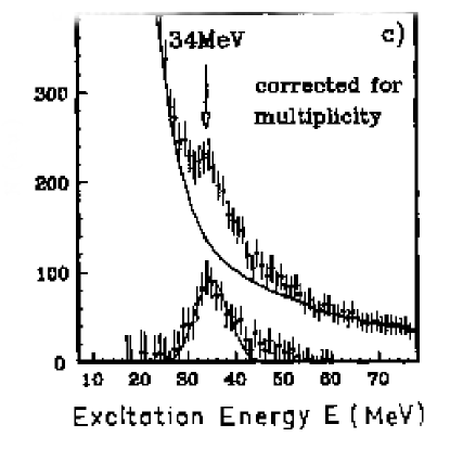
Figure 2.3: Experimental inelastic spectrum corrected for the proton multiplicity for the ⁴⁰Ca +⁴⁰Ca reaction at 44 MeV/n. The bump at 34 MeV corresponds to the double phonon giant quadrupole resonance. From [11].

⁴⁰Ca The main difficulty is the extraction of the structure from the background, whose characteristics are inevitably affected by uncertainties on the correction function.

GSI Interest in this subject has been renewed by recent experiments with relativistic heavy-ion beams at GSI, where inelastic cross sections for the excitation of the dipole DGR have been precisely measured. In fig. 2.4 we report the findings of the LAND collaboration (Large Area Neutron Detector). A structure at 28 $\pm$ 1 MeV is clearly observed with a width of about 6 $\pm$ 2 MeV and it is interpreted as a two phonon state, namely a double-GDR. The cross section for this state is measured to be 175 $\pm$ 50 mb.

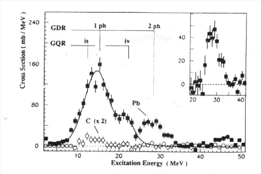
Figure 2.4: Experimental inelastic spectra for ¹³⁶Xe on ²⁰⁸Pb (black squares) at 700 MeV/n and on ¹²C (white circles, multiplied by 2). This figure is taken from [11], for more details see [13].

¹³⁶Xe²⁰⁸Pb ¹²C

The theoretically calculated cross sections – when performed within the framework of the standard harmonic model – systematically underestimate the experimental data by as much as a factor of two. This unexpected enhancement of the cross sections puts in evidence shortcomings in either the description of the structure of the modes or in the formulation of the reaction mechanism. Attempts to improve over this situation have followed different paths.

Another experiment has been performed for ²⁰⁸Pb on ²⁰⁸Pb at 640 MeV/n [14]. In this case the double phonon GDR is found at about 23.8 MeV with a width of about 6 MeV and a cross section of about 350 mb. Again this value is a factor of two larger that the prediction.

The microscopic understanding of these resonances, for instance, has been taken beyond the simple superposition of the 1p-1h configurations to include couplings to 2p-2h, 3p-3h and/or states of higher complexity [15, 16, 17]. Residual interactions give rise to anharmonicity in the energy spectrum [18] and, also, appreciable changes in the structure of the wave functions. Recently, a systematic study of the anharmonicity in the dipole DGR has been carried out for several nuclei [19]. This study, based on the QRPA quasiparticle RPA, has shown an effect of few hundred keV. The same order of magnitude had been found in ref. [20] for ²⁰⁸Pb and ⁴⁰Ca. These effects have been taken into ²⁰⁸Pb⁴⁰Ca account in macroscopic models that add small anharmonic contributions [21, 22] to the otherwise harmonic hamiltonian in the presence of an external time-dependent field. Depending on the magnitude of these anharmonic terms the inelastic cross sections for the population of the dipole DGR can reach values which are close to the experimental data. Microscopic calculations in the context of the RPA approximation,RPA have also succeeded in reducing the discrepancy between the experimental data and the theoretical predictions down to the level of a few per cent [20]. Another approach to the problem that has been examined [24, 25] exploits the so-called Brink-Axel hypothesis [23]. Brink-Axel hypothesis It also seems possible, through this formalism, to obtain enhancements in the population of states in the energy range around the DGR.

In this chapter we investigate the role of the nuclear coupling in the excitation of GR’s and DGR’s and its interplay with the long-range Coulomb excitation mechanism. Furthermore, we study the consequences of the spreading of the strength distribution of the single giant resonance on the inelastic cross section for both the GR and DGR. These topics have been previously explored in the literature. In refs. [26, 27, 28] nuclear and Coulomb interactions where taken into account for medium-heavy nuclei at low bombarding energy (around 50 MeV/A). While these studies put in evidence interference effects between the two excitation mechanisms there was no clear resolution concerning what could be actually attributed to each of them. Also, the role played by the resonances’ width on the reaction cross sections was covered in refs. [29, 30, 25]. The analysis, however, were done only for the case of the Coulomb excitation mechanism and lead to somewhat ambiguous results.

We will carry on this survey within a simple reaction model that has the virtue of conforming to the standard treatment of inelastic excitations which is familiar to many active participants in this field. Our original intention was limited to investigate the qualitative dependence of the probabilities of excitation of the Double Giant Resonances as a function of several global parameters such as the excitation energies, bombarding energies, multipolarity, anharmonicity, width, etc. In the process of refining the computer programs we used to obtain these global trends we ended up with a quite transparent and yet powerful tool that – we believe – can be useful for the experimentalists to make quantitative predictions for measurements in a wide variety of circumstances. With this very practical purpose in mind we shall take the width of the states as a free parameter. We shall also limit our calculations to the non-relativistic regime and, for the different examples, consider the excitation of single- and double-phonon Giant Quadrupole Resonances.

Following this Introduction we describe in Sect. 2.2 the formalism employed to make our estimates. Relevant results for the reaction ⁴⁰Ar + ²⁰⁸Pb are given with illustrations in Sect. 2.3. The conclusions that can be inferred from these examples are also the subject of this Section. Some concluding remarks are left for Sect. 2.4. ⁴⁰Ar ²⁰⁸Pb

2.2 The model

The excitation processes of the one and two-phonon states are calculated within the framework of the standard semiclassical model of semiclassical model Alder and Winther [31] for energies below the relativistic limit. According to this model for heavy ion collisions, the nuclei move along a classical trajectory determined by the Coulomb plus nuclear interaction. We will explore the energy range from few MeV up to hundreds of MeV per nucleon. During their classical motion the nuclei are excited as a consequence of the action of the mean field of one nucleus on the other. The excitation processes are described according to quantum mechanics and they are calculated within perturbation theory.

We assume that the colliding nuclei have no structure except for the presence, in the target, of one and two-phonon states whose energies are $E_{1}$ and $E_{2}=2E_{1}$, respectively. For the ion-ion potential we have used the Coulomb potential for point charged particles and the Saxon-Woods parametrization of the proximity potential $U_{N}(r)$ that are commonly used in heavy ion collisions [32].

In the theory of multiple excitations the set of coupled equations describing the evolution of the amplitudes in the different channels can be solved within the perturbation theory. We can write the probability amplitude to excite the $\mu$ component of the one-phonon state with multipolarity $\lambda$ as

$$a^{(1)}_{\lambda\mu}(t)=(-i/\hbar)\int_{-\infty}^{\infty}dtF_{\lambda\mu}(r(t),\hat{r}(t))e^{iE_{1}t/\hbar}~{},$$ (2.1)

where the integrals are evaluated along the classical trajectories ${\bf{r}}(t)$. In this equation the main ingredient is the coupling form factor

$$F_{\lambda\mu}(r(t),\hat{r}(t))~{}=~{}f_{\lambda}(r)~{}Y_{\lambda\mu}(\hat{r})~{},$$ (2.2)

chosen according to the standard collective model prescription [33]. For a given multipolarity $\lambda$ the radial part assumes the form

$$f_{\lambda}(r)={{3Z_{p}Z_{t}e^{2}}\over{(2\lambda+1)R_{C}}}\beta^{C}_{\lambda}\Bigg{(}{R_{C}\over r}\Bigg{)}^{\lambda+1}-\beta^{N}_{\lambda}R_{T}{d\over dr}U_{N}(r)~{}.$$ (2.3)

The deformation parameters $\beta$ determine the strength of the couplings, and they are normally directly associated with the $B(E\lambda)$ transition probability. The expression for the nuclear component of the form factor is not valid for $\lambda=1$. In this case the inelastic form factor is obtained from the Goldhaber-Teller or Jensen-Steinwendel models. The $Z_{p}$ ($Z_{t}$) denotes the charge number of the projectile (target), while $R_{C}$ and $R_{T}$ are the Coulomb and matter radii of the target nucleus.

In a similar way, the amplitude for populating the two-phonon state with angular momentum $L$ and projection $M$ can be obtained as

$$a^{(2)}_{LM}(t) = (1/\hbar)^{2}\sum_{\mu}~{}\sqrt{(1+\delta_{\mu,M-\mu})}$$ (2.4)

$$\times \int_{-\infty}^{\infty}dtF_{\lambda,M-\mu}({\bf r}(t))e^{i(E_{2}-E_{1})t/\hbar}\int_{-\infty}^{t}dt^{\prime}F_{\lambda,\mu}({\bf r}(t^{\prime}))e^{iE_{1}t^{\prime}/\hbar}$$

Solving the classical equation of motion we can calculate for each impact parameter $b$ the excitation probability $P^{(1)}(b)$ and $P^{(2)}(b)$ to populate the single- and the double-phonon state. These are given by

$$P^{(1)}(b)~{}=~{}\sum_{\mu}|a^{(1)}_{\lambda\mu}(t=+\infty)|^{2}$$ (2.5)

and

$$P^{(2)}(b)~{}=~{}\sum_{L}P^{(2)}_{L}~{}=~{}\sum_{LM}|a^{(2)}_{LM}(t=+\infty)|^{2}~{}.$$ (2.6)

In order to get the corresponding cross sections we have then to integrate the probabilities $P^{(\alpha)}$’s ($\alpha$ =1,2)

$$\sigma_{\alpha}=2\pi\int_{0}^{\infty}P^{(\alpha)}(b)T(b)bdb\,.$$ (2.7)

Generally, in Coulomb excitation processes the transmission coefficient is taken equal to a sharp cutoff function $\theta(b-b_{min})$ and the parameter $b_{min}$ is chosen in such a way that the nuclear contribution is negligible. We want to take into account also the contribution of the nuclear field so in our case T(b) should be zero for the values of $b$ corresponding to inner trajectory and then smoothly going to one in the nuclear surface region. This can be naturally implemented by introducing an imaginary term in the optical potential which describes the absorption due to non elastic channels. Then the survival probability associated with the imaginary potential can be written as

$$T(b)=\exp\Bigg{\{}{2\over\hbar}\int_{-\infty}^{+\infty}W(r(t))dt\Bigg{\}}\,,$$ (2.8)

where the integration is done along the classical trajectory. The imaginary part $W(r)$ of the optical potential was chosen to have the same geometry of the real part with half its depth.

The excitation processes of both single and double GR can change significantly when one takes into account the fact that the strength of the GR is distributed over an energy range of several MeV. Among the few standard choices for the single GR strength distribution, we will assume a Gaussian shape, with a width $\Gamma_{1}=2.3\sigma$ which we will take as a parameter, of the following form

$$S(E)={1\over{\sqrt{2\pi}\sigma}}\exp\Bigg{\{}{-(E-E_{1})^{2}\over{2\sigma^{2}}}\Bigg{\}}\,.$$ (2.9)

Calculations have been also performed with a Breit-Wigner shape yielding similar trends. However, the Gaussian form guarantees a better localization of the response and prevents superposition of the modes for the largest widths (for a further discussion see ref. [17]).

To get the cross section to the one-phonon state one then defines a probability of excitation per unit of energy,

$$dP^{(1)}(E,b)/dE~{}=S(E)~{}\sum_{\mu}|a^{(1)}_{\lambda\mu}(E,t=+\infty)|^{2}~{},$$ (2.10)

where the single amplitudes $a^{(1)}_{\lambda\mu}(E,t)$ are obtained as before, but with a variable energy $E$. The probability of exciting the double-phonon state is then obtained by folding the probabilities of single excitation, in the form

$$dP^{(2)}(E,b)/dE~{}=~{}\int dE^{\prime}~{}{dP^{(1)}(E^{\prime},b)\over dE}~{}~{}{dP^{(1)}(E-E^{\prime},b)\over dE}~{}.$$ (2.11)

The total cross section for one- and two-phonon states can then be constructed as

$$\sigma_{\alpha}=2\pi\int_{0}^{\infty}\int_{0}^{\infty}{dP^{\alpha}\over dE}(E,b)~{}T(b)\,b\,db\,dE\,\,.$$ (2.12)

Due to the Q-value effect it is clear that one expects a distortion in the shape of the distribution of the cross section which will favor the lower part of the distribution in energy.

2.3 Results

We show in fig. 2.5 the dependence on the impact parameter of the excitation probabilities for the one- and two-phonon states of the Giant Quadrupole Resonance giant quadrupole resonance in lead. The reaction we have chosen for ⁴⁰Ar ²⁰⁸Pb this illustration is ⁴⁰Ar + ²⁰⁸Pb at a bombarding energy of 40 MeV per nucleon. The deformation parameters have been chosen equal $\beta^{C}=\beta^{N}=0.07$, in agreement with the currently estimated value for the $B(E2)$. The range of impact parameters given in the figure covers the relevant grazing interval, and in a classical picture (including both Coulomb and nuclear fields) yields scattering angles between $3.4$ and $5.5$ degrees. In the strictly harmonic case the probabilities for excitation of the double-phonon state can of course be constructed from those corresponding to the single-phonon; they are both explicitly given here for a matter of later convenience. Each frame displays a set of three curves that allows us to compare the individual contributions of the Coulomb and nuclear fields to the excitation process and put in evidence a value of $b\approx 12.5$ fm for the maximum (destructive) interference between the competing mechanisms.

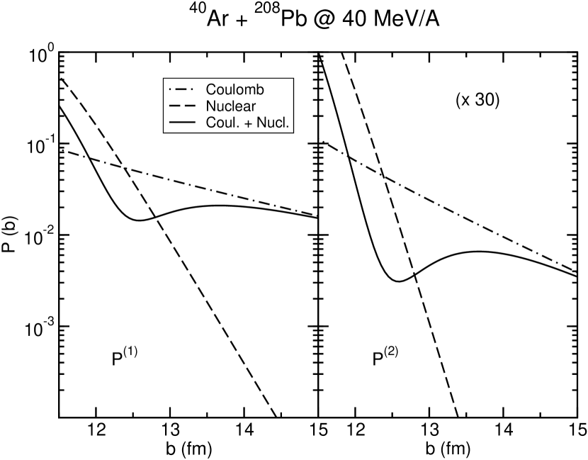
Figure 2.5: Excitation probability vs. impact parameter for the one- (left part) and two-phonon (right part) states of the GQR in lead for the reaction ⁴⁰Ar + ²⁰⁸Pb at 40 MeV/A. The Coulomb (dot-dashed line) and nuclear (dashed) probabilities are displayed as well as the total (solid line). The curves on the right part have been multiplied by 30.

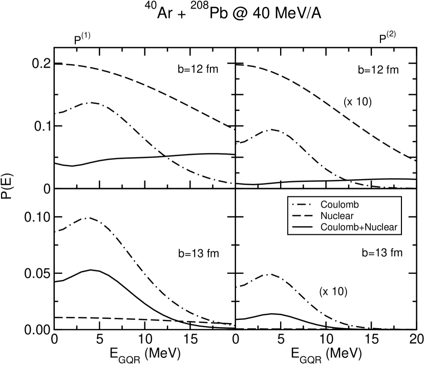
Figure 2.6: Excitation probabilities as function of the GQR energy, which is taken as a parameter, for the reaction ⁴⁰Ar + ²⁰⁸Pb at 40 MeV/A. The graphs on the left correspond to the excitation probability of the single GQR ($P^{(1)}$) while the ones on the right correspond to DGQR ($P^{(2)}$) and they are multiplied by a factor 10. The Coulomb (dash-dotted line) and nuclear (dashed) probabilities are displayed as well as the total (solid line). The upper (lower) figures correspond to an impact parameter of 12 (13) fm.

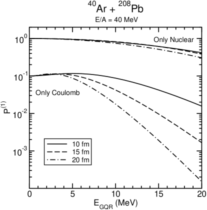
Figure 2.7: Excitation probability for the single GQR as a function of the GQR energy for three values of impact parameters. They have been normalized to their values at $E_{GQR}=0$. The upper curves correspond to the excitation probability due only to the nuclear field. The probabilities calculated only with the Coulomb field are shown in the lower part of the picture. They have been divided by 10 in order to render the figure readable.

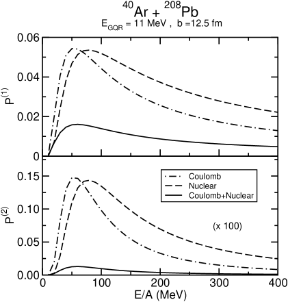
Figure 2.8: Excitation probability as a function of incident energy of the one- (upper part) and two-phonon (lower part) states of the GQR in lead for the reaction ⁴⁰Ar + ²⁰⁸Pb for an impact parameter of 12.5 fm. The Coulomb (dot-dashed line) and nuclear (dashed) probabilities are displayed as well as the total one (solid line). The curves on the lower part have been multiplied by 100.

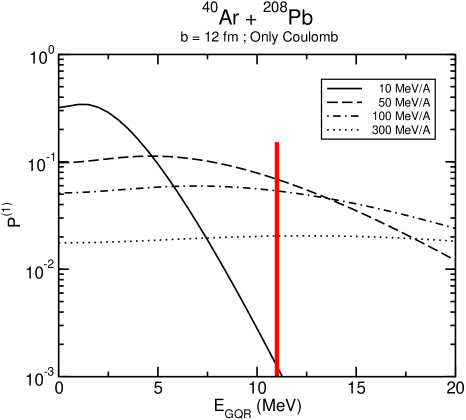
Figure 2.9: Coulomb excitation probability for the one-phonon state as a function of the Q-value and for four different incident energies as shown in the legend. The curves correspond to calculations done for an impact parameter b=12 fm. The vertical line indicates the GQR energy for lead.

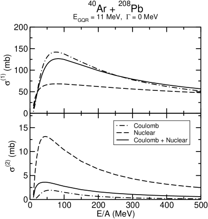
Figure 2.10: Excitation cross section for the GQR (upper figure) and DGQR state (lower figure) as a function of the incident energy. Again, the Coulomb (dot-dashed line), nuclear (dashed line) and total (solid line) contributions are shown.

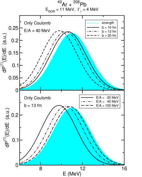
Figure 2.11: Normalized distributions of Coulomb excitation probability for the one-phonon state for different impact parameters (upper figure) and bombarding energies (lower figure) as shown in the legend. The shaded area shows the Gaussian strength distribution used as input in the calculation. The width has been chosen to be 4 MeV.

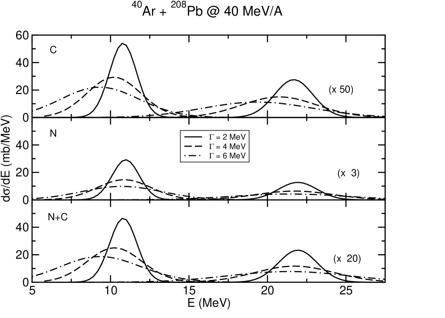
Figure 2.12: Cross section distribution for the reaction ⁴⁰Ar + ²⁰⁸Pb at 40 MeV/A for three values of the width as indicated in the legend. The contributions of the Coulomb (C), nuclear (N) and total (N+C) cross sections are shown in single graphs. The cross sections for DGQR are multiplied by the factors reported in the figure.

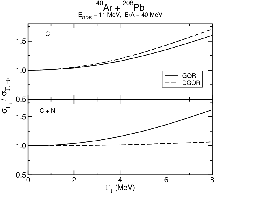
width

Figure 2.13: Total cross sections for the excitation of GQR (solid line) and of DGQR (dashed line) as a function of the strength distribution width $\Gamma_{1}$ of the single GQR for the reaction ⁴⁰Ar + ²⁰⁸Pb at $30MeV/A$. In the graphs we report the cross sections due to the Coulomb field (upper) and total (lower), each of them divided by their corresponding value for sharp distribution ($\Gamma_{1}=0$). We have not reported the nuclear contribution because the cross sections for both GQR and DGQR do not change appreciably when a finite distribution is assumed.

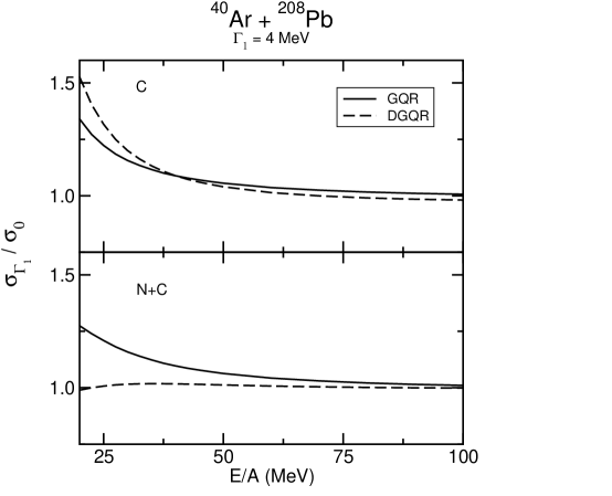
Figure 2.14: Same as fig. 2.13 as a function of the bombarding energy. The strength distribution width has been chosen equal to 4 MeV.

We use the same reaction as in fig.2.5 to illustrate the effect of the reaction Q-values on the transition probabilities. The dependence of the single-step inelastic excitation to the one-phonon state of energy $E_{{}_{GQR}}$ and the sequential process feeding the double-phonon state at twice this value are shown in fig.2.6. As before, the three curves in each frame display the separate contributions of the Coulomb and nuclear fields and the combined total. Two values of the impact parameter have been chosen specifically to cover a situation of nuclear ($b$=12 fm) and Coulomb ($b$=13 fm) dominance. The results show – even in a linear scale – a somewhat moderate dependence with the frequency of the mode. This is due to the relatively high bombarding energy chosen in this example, for which the time-dependence of both the Coulomb and nuclear excitation fields are quite well-tuned to the intrinsic response.

There is a qualitative difference in the effective collision time for Coulomb and nuclear inelastic processes that is worth mentioning. We refer to the dependence, for a given bombarding energy, of the excitation probabilities for the one- and two-phonon states on the impact parameter. Because of the long range of the formfactors the change of the effective collision time $\tau$ for Coulomb excitation follows a different law than the one corresponding to the nuclear inelastic processes. It can be estimated that $\tau_{{}_{C}}/\tau_{{}_{N}}\approx A_{\lambda}\sqrt{b}$, where the proportionality factor $A_{\lambda}$ is a monotonically decreasing function of the multipolarity $\lambda$. For all multipolarities, however, $\tau_{{}_{C}}$ is larger than $\tau_{{}_{N}}$. It follows from these arguments that the adiabatic cut-off function that affects the transition amplitudes for Coulomb excitation varies significantly over the large range of impact parameters that contributes to this process. For the nuclear field a favorable matching between effective collision times and the intrinsic period of the mode applies, on the other hand, to most of the relevant partial waves. This can be understood by examining fig. 2.7 , where the probability for excitation of the one-phonon level is plotted as a function of the energy of the mode for three impact parameters, $b$=10, 15 and 20 fm. Two sets of curves are shown, corresponding to Coulomb and nuclear excitation only. In both instances the probabilities are normalized to their values for $E_{{}_{GQR}}$=0 MeV to emphasize the different character of the response. Notice, for instance, that for $E_{{}_{GQR}}$=20 MeV the role of the Coulomb field for $b$=20 fm would be effectively quenched by two orders of magnitude in spite of its long range. (This is of course in addition to the gradual reduction of the transition amplitudes caused by the slow $r^{-(\lambda+1)}$ dependence of the couplings.)

We use fig.2.8 to illustrate the dependence of the excitation probabilities upon the bombarding energy. For this we take a value of $E_{{}_{GQR}}$=11 MeV, close to the actual excitation energy of the Giant Quadrupole Resonance in lead. The impact parameter $b$ is set to 12.5 fm, which provides the condition in which the importance of the Coulomb and nuclear excitations become comparable. Of course it is also the choice of impact parameter that yields the maximum (negative) interference between the two reaction mechanisms. What we see is a rapid increase of the probabilities for the one-phonon and two-phonon levels up to a bombarding energy of about 50 MeV/nucleon. After that a gradual decline sets in up to about 400 MeV/nucleon, an energy beyond which a relativistic formalism must be implemented. The trend, however, is not to be significantly altered and, in view of these results one cannot but wonder about the actual need of exploiting relativistic bombarding energies to probe the excitation of double-phonon giant resonances in nuclei. In principle, and entirely from an adiabatic point of view, the higher the bombarding energy the better. Yet, optimal matching conditions reach saturation and one cannot ignore the fact that, beyond this point, one can no longer expect a further enhancement of the excitation probabilities. Quite on the contrary, the interaction time is effectively reduced up to a point where (as the figure shows) the excitation of the modes becomes less and less favored (see caption to fig. 2.9 and, also, ref. [30]).

In fig.2.10 we display the cross section for the excitation of the GQR and DGQR as a function of the bombarding energy in MeV per nucleon. This observable quantity combines the effect of all impact parameters and the plot puts in evidence a quite interesting feature. Notice that at all bombarding energies the population of the one-phonon state is dominated by the Coulomb formfactors. At the two-phonon level, on the other hand, it is mostly the nuclear coupling that determines the outcome. To understand the origin of this exchange of roles it may be helpful to re-examine fig.2.5. We have here to pay attention to the dependence of the ratio between the probabilities for nuclear and Coulomb excitation in the relevant range of impact parameters, 11-13 fm. (To this end the display factor of 30 introduced for the case of the two-phonon state is of no consequence.) The enhanced logarithmic slopes for the DGQR resulting from the squaring of the one-phonon probabilities suffice to give the leading edge to the nuclear couplings. This realization has major consequences insofar as the global properties of the excitation of the GQR and DGQR is concerned. In fact, the transition probabilities will inevitably reflect the different characteristics of the reaction mechanism that it is mostly responsible for the population of one state or the other.

Q-value considerations have such a pronounced effect on the excitation probabilities that it is clear that they will play an important role when one takes into account the sizable width of the one- and two-phonon states. Suppose that instead of having the total strength of the mode at a fixed value $E_{{}_{GQR}}$ we distribute it with the profile of a Gaussian distribution of width $\Gamma$. If the energy of the mode is quite off the optimal Q-value window one should expect that the distribution of measured cross sections will follow a quite different law. In fact, whenever the dynamic response in the vicinity of $E_{{}_{GQR}}$ is a rapidly changing function of the energy (see, for instance, fig. 2.9 for $E$=10 MeV/A) the experimental distribution will be significantly distorted and shifted toward lower energies. We illustrate this aspect in fig. 2.11, where the distribution of Coulomb excitation probabilities for the one-phonon state, $dP^{(1)}/dE$, is shown for different impact parameters and bombarding energies. In each frame the shaded curve shows the Gaussian distribution of strength that is the input to the calculation. Notice that all distributions have been normalized in order to emphasize the effect of interest and to eliminate the over-all dependence on $b$ and $E$ discussed earlier. As it follows from our considerations one can easily see that the smaller distortion corresponds indeed to the smaller impact parameters and/or the larger bombarding energies.

width The distortion of the line profile at the one-phonon level increases as a function of the width $\Gamma$, as it is clearly seen in fig. 2.12, where reaction cross sections (i.e. the result of an integration over impact parameters) are shown for a typical value of the bombarding energy. For the larger width $\Gamma$=6 MeV the apparent shift of the distribution is large enough as to place most of the cross section outside of the initial range set by the Gaussian curve. The effect seems to be more noticeable at the two-phonon level, as shown on the right-hand-side of the figure. According to our previous discussion, it is the Coulomb excitation mechanism that contributes most to the difference between the strength and cross section profiles.

From the energy distributions displayed in fig.2.12 one can calculate the total one- and two-phonon cross sections, by integrating over the excitation energy. The global effect of the finite width is shown in fig. 2.13, where the total cross sections for different values of the width are compared with the corresponding values for sharp resonances. The enhanced excitation in the lower part of the distribution leads to a global enhancement in the case of the Coulomb field. As a consequence, a corresponding enhancement is present in the combined Coulomb+nuclear case in the one-phonon excitation, which is dominated by the Coulomb interaction. On the contrary, being the two-phonon cross section predominantly due to the nuclear process, no appreciable variation is predicted for this case with finite values of the width.

Since the effect of the width arises from the Q-value kinematic matching conditions, variations are expected with the bombarding energy. In particular one expects that the effects will tend to vanish at high bombarding energies. This is illustrated in fig. 2.14, where the total one- and two-phonon cross sections for $\Gamma$ = 4 MeV are compared to the corresponding values for $\Gamma$ = 0 as a function of the incident energy.

2.4 Conclusions and remarks

We have implemented a simple scheme to calculate the excitation probabilities for the single and double Giant Resonance as a function of several global parameters such as excitation energies, bombarding energies, width etc. We have assumed that the colliding nuclei have no structure except for the presence, in the target, of one and two-phonon states. The excitation processes have been calculated within a semiclassical model and according to perturbation theory. Since both nuclear and Coulomb interaction are taken into account the cross sections are calculated by integrating over all range of impact parameter with an imaginary potential that takes care of the inner trajectories. The formalism has been applied to the excitation of giant resonances in a typical heavy ion reaction, ⁴⁰Ar + ²⁰⁸Pb. In our examples, we have limited our calculation to the giant quadrupole resonance.

The role of the nuclear interaction and its interplay with the long-ranged Coulomb field has been studied. The presence of nuclear coupling modifies the mechanism excitation of both the GR and the DGR, the effect being strongly evident in the latter. This has been ascribed to the difference in the effective collision time which, together with the qualitative $r$ dependence of the form factors, produces a different dependence of the transition probabilities on the reaction Q-value. Hence, the excitation of GR is dominated by the Coulomb interaction while it is mostly the nuclear coupling which determines the population of the DGR.

We have also studied the consequences of the spreading of the strength distribution of the single giant resonance on the inelastic excitation of the GR and DGR. Q-value considerations play an important role when the width of the one- and two-phonon states are considered. Cross section dependence on both the width of the distribution and the incident energy has been considered. When compared with the corresponding values for sharp resonances, the cross sections for GR and DGR calculated with only the Coulomb field increase as $\Gamma$ increases. These results are qualitatively similar to the one obtained in ref. [25] where the relativistic Coulomb excitation of dipole giant resonance (GDR) and double GDR are calculated within a random matrix theory including the Brink-Axel hypothesis. When the nuclear interaction is switched on, the enhancement for the single GR is maintained while the two-phonon cross section presents no variation with the case of finite value of the width. Also for the dependence on the incident energies has been found the same trend. This is due to the fact that the two-phonon cross section is predominantly governed by nuclear processes.

Chapter 3 Giant Pairing Vibrations

3.1 Introduction.

Conventional giant resonances, that have been discussed in the last chapter and that will form the subject of the fourth chapter, may be considered as collective modes where a significant part of the constituents of the nucleus oscillates or moves together. In a microscopic picture giant resonances, corresponding to surface vibrations, can be viewed as coherent particle-hole excitations to high-lying states, where the transition matrix elements receive in-phase contributions from all the various possible configurations. The amount of collectivity is determined by the values of the matrix elements of the appropriate transition operator.pp-RPA In this chapter we will concentrate on a collective mode of a different kind, that nevertheless may be studied exploiting a number of analogies with the well-known case. The formal analogy between particle-hole and particle-particle excitations is well established as well as the use of a one-body pair field (see fig. 3.1 for a schematic illustration) and may be brought to the concept of high-lying two particle excitation (populated via two-particle transfer reactions). In this way the giant mode acquires its collectivity from the coherent superposition of all the possible two-particle configurations. This mode is called Giant Pairing Vibration Giant Pairing Vibration and is created by the action of the pairing field in the very same way in which low-lying 0⁺ pairing vibrations are encountered in the excitation of closed shell nuclei and their vicinity. The analogy between shape rotations and vibrations and pairing rotations and vibrations may be carried quite far. In closed shell nuclei strongly enhanced $L=0$ transitions manifest themselves following a vibrational pattern, in which a pair of transferred particle change the number of phonons by one, and two types of phonons are present because two nucleons can either be added or removed). In mid-shell nuclei a series of ground state transitions is seen between monopole states that follows a rotational scheme. While the low-lying pairing states have been sistematically seen, the corresponding giant mode is still awaiting an experimental confirmation. Certainly these states are embedded in the continuum and the large background produced by other states, with all possible multipolarities, makes difficult their identification in experiments. pair field

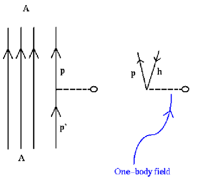
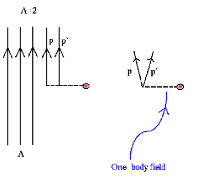
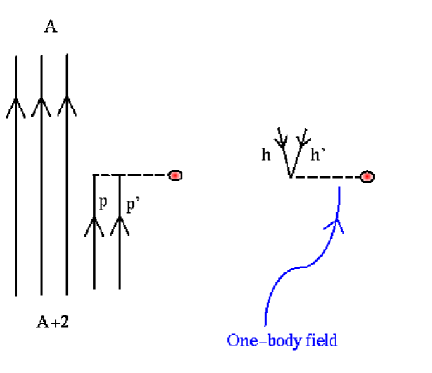
a b c

Figure 3.1: Formal analogy between particle-hole (a) and particle-particle (b) or hole-hole (c) excitations. The one body field that acts in the last two cases is the pairing field.

Large efforts have been recently dedicated to the study of different aspects of reaction mechanism in collisions induced by weakly-bound radioactive beams. The long tails of the one-particle transfer form factors due to the weak binding, associated with the possibility of unusual behaviour of pairing interaction in diluted systems, has raised novel interest in the possibility of studying the pair field via two-particle transfer processes with unstable beams [34]. On the other hand, in transfer reactions induced by weakly bound projectiles on stable targets, the Q-values for the low-lying states will be very large (typically of the order of 10-15 MeV for the (⁶He,⁴He) stripping reaction). This will strongly hinder these processes ⁶He for reactions where the semi-classical optimum matching conditions apply, as it is the case of bombarding energies around the Coulomb barrier on heavy target nuclei. Higher bombarding energies, where the matching conditions are less stringent, may on the other hand not be suitable because of large break-up cross sections. The same matching conditions will favour instead the population of highly excited states, as the Giant Pairing Vibrations (GPV), and the use of Radioactive Ion Beams (RIB) Giant Pairing Vibration may therefore become instrumental in offering the opportunity of studying nuclear structure aspects that are not usually accessible with stable projectiles. These Giant Pairing Vibrations are in fact predicted [35] to have strong collective features, but their observation may have so far failed [36] because of large mismatch in reactions induced by protons or tritons, at variance to the case of the low-lying pairing vibrations, which have been intensively and successfully studied around closed shell nuclei in two-particle transfer reactions [37]. All these 0⁺ states are associated with vibrations of the Fermi surface and are described in a microscopic basis of the shell model as correlated two particle- two hole states. In the case of the Giant Pairing Vibrations the excitation involves the promotion of a pair of particles (or holes) in the next major shell (hence an excitation energy around 2$\hbar\omega$) and is expected to display a collective pairing strength comparable with the low-lying vibrations. The predicted concentration of strength of a $L=0$ character in the high-energy region (8-15 MeV for most nuclei) is understood microscopically as the coherent superposition of 2p (or 2h) states in the next major shell above the Fermi level. With a Random Phase Approximation in mind (or even with a simpler Tamm-Dancoff approximation), one may solve the secular problem for an hamiltonian consisting simply of a kinetic operator. All the possible energies obtained by placing two particles in the obtained single-particle energy level scheme may be called unperturbed energies. Once a pairing interaction (with constant strength, to fix the ideas) is added to this hamiltonian the solution of the secular equation may be drawn and the corresponding dispersion relation may be depicted as in Fig. (3.2). The Giant Pairing Vibration is the collective mode that is seen in the energy gap between the first and the second major shell.

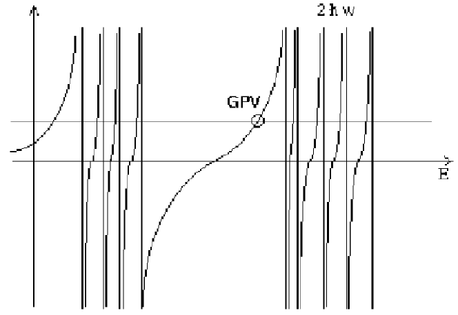
Figure 3.2: Raw picture of the dispersion relation. The two bunches of vertical lines represent the unperturbed energy of a pair of particles placed in a given single particle energy level. The graphical solutions of the secular equation are the intersection of the horizontal line ($1/G$) with the curves. The GPV is the collective state relative to the second major shell.

Also in the case of superfluid superfluid systems in an open shell the system is expected to display a collective high-lying state, that in this case collects its strength from the unperturbed two-quasiparticle 0⁺ states with energy 2$\hbar\omega$. To investigate this possibility we made estimates of cross sections to the Giant Pairing Vibrations in two-particle transfer reactions, comparing the cases of bound or weakly-bound projectiles. ¹⁴C As examples we have considered the case of (¹⁴C,¹²C), from one side, and the case of (⁶He,⁴He) as representative of a reaction induced by a weakly-bound ion. As targets, we have chosen the popular cases of the lead and tin regions (so considering both “normal” and “superfluid” nuclei). To perform the calculation, we will first evaluate the response to the pairing operator in the RPA, including both the low-lying and high-lying pairing vibrations. As a following step we will then construct two-neutron transfer form factors, using the “macroscopic” model for pair-transfer processes. Finally, estimates of cross sections will be given using standard DWBA DWBA techniques. As we will see, in the case of the stripping reaction induced by ⁶He, the population of the GPV is expected to display cross sections of the order of a millibarn, dominating over the mismatched transition to the ground state.

This chapter is organized as follows. In the next section we discuss the theoretical formalism used for normal and for superfluid nuclei. In section 3.3 we recall the basics aspects of the macroscopic form factors for two-particle transfer reactions and in section 3.4 we display the results of calculations for the paradigmatic examples of ²⁰⁸Pb and ¹¹⁶Sn.

3.2 The pairing response and the Giant Pairing Vibration.

pair field A simple way of displaying the amount of pairing correlations is in terms of the pair transfer transition densities [38]. These are defined as matrix elements of the pair density operator connecting the ground state in nucleus $A$ with the generic $0^{+}$ state $|n\rangle$ in nucleus $A\pm 2$, namely

$$\delta\rho_{P}(r)=\langle n|\hat{\rho}_{P}|0\rangle,$$ (3.1)

where the generalized density operator is given by

$$\hat{\rho}_{P}(r)=\sum_{\alpha}{\sqrt{2j+1}\over{4\pi}}R_{\alpha}(r)R_{\alpha}(r)([a_{\alpha}^{\dagger}a_{\alpha}^{\dagger}]_{00}+[a_{\alpha}a_{\alpha}]_{00}).$$ (3.2)

Here $R_{\alpha}(r)$ are the radial wave functions of the $\alpha=\{nlj\}$ level and the sum runs over both particle and hole levels. The pair transfer strength to each final state can be obtained from the corresponding pair transfer transition density by simple quadrature, namely

$$\beta_{P}=\int 4\pi r^{2}\delta\rho_{P}dr.$$ (3.3)

For normal systems around closed shell the strong L=0 transition follows a vibrational scheme, where the correlated pair of fermions (pairing phonon) change by one [39]. In this case, there are two types of phonons associated with the stripping and pick-up reactions. The two-particle collective state is called ”addition” pairing phonon while the two-holes correlated state is known as ”removal” pairing phonon. From a microscopic point of view the two kind of phonons, corresponding to the $(A\pm 2)$ nuclei can be described in terms of the two-particle (two-hole) states of the Tamm Dancoff Approximation(TDA) or in a better way by a Random Phase Approximation (RPA). RPA We start from a hamiltonian with a Monopole Pairing interaction:

$$H=\sum_{j}\epsilon_{j}a^{\dagger}_{j}a_{j}-G4\pi P^{\dagger}P,$$ (3.4)

where

$$P^{\dagger}=\sum_{j_{1}\leq j_{2}}{M(j_{1},j_{2})\over\sqrt{1+\delta_{j_{1}j_{2}}}}\left[a^{\dagger}_{j_{1}}a^{\dagger}_{j_{2}}\right]_{00}.$$ (3.5)

Here the $a^{\dagger}_{j}$ creates a particle in an orbital $j$, where $j$ stands for all the needed quantum numbers of the level. The constant $G$ is the strength of the pairing interaction and the coefficients $M(j_{1},j_{2})$ are:

$$M(j_{1},j_{2})={\langle j_{1}||f(r)Y_{00}(\theta,\phi)||j_{2}\rangle\over\sqrt{1+\delta_{j_{1}j_{2}}}},$$ (3.6)

where the detailed radial dependence of $f(r)$ is taken to be of the form $r^{L}$ and in our case is a constant since we are dealing only with $L=0$ states. The pairing phonons, that is to say the quanta associated with the two collective modes of the above hamiltonian, are defined for closed shell nuclei as:

$$\begin{array}[]{lll}|n,2p\rangle=\Gamma_{n,2p}^{\dagger}|0\rangle_{RPA}=&{}&{}\\ \qquad=\Bigl{(}\sum_{k}X_{n}(k)[a^{\dagger}_{k}a^{\dagger}_{k}]_{00}+\sum_{i}Y_{n}(i)[a_{i}^{\dagger}a_{i}^{\dagger}]_{00}\Bigr{)}\mid 0\rangle_{RPA}&{}&{}\\ &&\\ |n,2h\rangle=\Gamma_{n,2h}^{\dagger}|0\rangle_{RPA}=\Gamma_{n,2p}|0\rangle_{RPA}&{}&{}\\ \qquad=\Bigl{(}\sum_{i}X_{n}(i)[a_{i}a_{i}]_{00}+\sum_{k}Y_{n}(k)[a_{k}a_{k}]_{00}\Bigr{)}\mid 0\rangle_{RPA}&{}&~{},\\ \end{array}$$

where $k(i)$ stands for levels above (below) the Fermi level. The index $j$ runs over both particle and hole levels. We have indicated with $\mid 0\rangle_{RPA}$ the correlated RPA vacuum. It represents the ground state with respect to the boson annihilation operator $\Gamma_{n,2h}^{\dagger}\mid 0\rangle_{RPA}=0$. The definitions of $X_{n}$ and $Y_{n}$ (called forward and backward amplitudes) are the standard ones and come from the solution of the RPA equation. They may be found in [39]. Within this model the pair transfer strength associated with each RPA state is microscopically given by

$$\beta_{Pn}=\sum_{j}\sqrt{2j+1}[X_{n}(j)+Y_{n}(j)].$$ (3.7)

In Fig. 1a we display the predicted pairing response in the case of ²⁰⁶Pb, namely two-neutron holes with respect to the double magic ²⁰⁸Pb. The set of single-particle levels that has been used in the RPA calculation, was obtained using the spherical harmonic oscillator levels with corrections due to the centrifugal and spin-orbit interactions [40]

$${E\over{\hbar\omega}}=N+{3\over 2}-\mu\left(l(l+1)-{{N(N+3)}\over 2}\right)+K$$ (3.8)

$$K=\left\{\begin{array}[]{ll}-\kappa l&\mbox{ for }j=l+1/2\\ -\kappa(l+1)&\mbox{ for }j=l-1/2\end{array}\right.,$$

where $\hbar\omega=41A^{-{1\over 3}}$, $A$ is the mass number of the nucleus, $N$ is the principal quantum number and $j,l$ are the total and orbital angular momentum quantum numbers, respectively. The quantities $\kappa$ and $\mu$ are parameters chosen to obtain the best fit for each nucleus [41]. We have included in the calculation all the single-particle levels starting from $N=0$ up to 10. This set is expected to be good enough for our calculation of the Giant Pairing Resonance, except for the levels around the Fermi surface. In the lead region we prefer to use experimental values for the shells just above and below the Fermi surface [52]. The Figure shows, in addition to the strong collectivity associated with the ground state transition, a strong collective state with about half of the g.s. strength at high excitation energy, around 16 MeV, which can be interpreted as the Giant Pairing Vibration. Similar situation is shown in Fig. 1b for the corresponding two-neutron addition states in the ²¹⁰Pb. Again one may interpret the strength at about 12 MeV as associated with the giant mode. Note that in both addition and removal cases, the contribution of the backward amplitudes to the wavefunction is found to be roughly equivalent to 5-10% in the ground state, while in the GPV this contribution reduces to less than 1%.

Figure 3.3: Pairing response for the removal (upper panel) and addition (lower panel) mode in ²⁰⁸Pb. The ground state transition and the candidate for GPV are evidenced.

We consider now the case of superfluid spherical-nuclei. In this case we make a BCS superfluid BCS transformation of the hamiltonian defined in Eq. [3.4] changing from particle to quasiparticle operators, introducing the usual occupation parameters. We start from a single-quasiparticle Hamiltonian plus a two-quasiparticle interaction corresponding to the residual $H_{22}+H_{40}$ of the pairing force

$$H=\sum_{j}E_{j}\alpha^{\dagger}_{j}\alpha_{j}+2\pi G\sum_{j_{1}j_{2}}M(j_{1},j_{1})M(j_{2},j_{2})\cdot$$

$$\cdot\Bigl{\{}(U^{2}_{j_{1}}U^{2}_{j_{2}}+V^{2}_{j_{1}}V^{2}_{j_{2}})[\alpha^{\dagger}_{j_{1}}\alpha^{\dagger}_{j_{1}}]_{00}[\alpha_{j_{2}}\alpha_{j_{2}}]_{00}-U^{2}_{j_{1}}V^{2}_{j_{2}}[\alpha^{\dagger}_{j_{1}}\alpha^{\dagger}_{j_{1}}]_{00}[\alpha^{\dagger}_{j_{2}}\alpha^{\dagger}_{j_{2}}]_{00}$$

$$-V^{2}_{j_{1}}U^{2}_{j_{2}}[\alpha_{j_{1}}\alpha_{j_{1}}]_{00}[\alpha_{j_{2}}\alpha_{j_{2}}]_{00}\Bigr{\}},$$ (3.9)

where

$$\alpha^{\dagger}_{j} = U_{j}a^{\dagger}_{j}-V_{j}a_{\bar{j}}$$ (3.10)

$$U^{2}_{j} = {1\over{2}}\left(1+{{\tilde{\epsilon}_{j}}\over E_{j}}\right)$$ (3.11)

$$V^{2}_{j} = {1\over 2}\left(1-{{\tilde{\epsilon}_{j}}\over E_{j}}\right).$$ (3.12)

The energies $E_{j}=\sqrt{{\tilde{\epsilon}}_{j}^{2}+\Delta^{2}}$ are the quasi-particle energies, and ${\tilde{\epsilon}_{j}}=\epsilon-\lambda$ are the single-particle energies with respect to the chemical potential $\lambda$ and $\Delta$ is the BCS gap. As usual we have defined $a_{\bar{j}}\equiv a_{\bar{jm}}=(-1)^{j-m}a_{j,-m}$.

For superfluid systems the addition and removal RPA phonons cannot be treated separately. The dispersion relation, that relates the strength of the interaction with the energy-roots of the RPA, becomes a two by two determinant. From the RPA equations:

$$\Gamma^{\dagger}_{n}~{}=~{}\sum_{j}\left(X_{n}(j)[\alpha^{\dagger}_{j}\alpha^{\dagger}_{j}]_{00}+Y_{n}(j)[\alpha_{j}\alpha_{j}]_{00}\right)$$ (3.13)

$$\left[H,\Gamma^{\dagger}_{n}\right]~{}=~{}\omega_{n}\Gamma^{\dagger}_{n},$$ (3.14)

$$\left[\Gamma_{n^{\prime}},\Gamma^{\dagger}_{n}\right]~{}=~{}\delta_{nn^{\prime}}$$ (3.15)

we can obtain the following factors

$$x = \sum_{j_{1}\leq j_{2}}|M(j_{1}j_{2})|^{2}\left[\frac{U^{2}_{j_{1}}U^{2}_{j_{2}}}{E_{j_{1}}+E_{j_{2}}-\omega_{n}}+\frac{V^{2}_{j_{1}}V^{2}_{j_{2}}}{E_{j_{1}}+E_{j_{2}}+\omega_{n}}\right]$$

(3.16)

$$y = \sum_{j_{1}\leq j_{2}}|M(j_{1}j_{2})|^{2}\left[\frac{V^{2}_{j_{1}}V^{2}_{j_{2}}}{E_{j_{1}}+E_{j_{2}}-\omega_{n}}+\frac{U^{2}_{j_{1}}U^{2}_{j_{2}}}{E_{j_{1}}+E_{j_{2}}+\omega_{n}}\right]$$

(3.17)

$$z = \sum_{j_{1}\leq j_{2}}|M(j_{1}j_{2})|^{2}(U_{j_{1}}V_{j_{2}}U_{j_{2}}V_{j_{1}})$$

$$\left[\frac{1}{E_{j_{1}}+E_{j_{2}}-\omega_{n}}+\frac{1}{E_{j_{1}}+E_{j_{2}}+\omega_{n}}\right],$$ (3.18)

and the dispersion relation is in this case:

$$\left|\matrix{(1-4\pi Gx)&4\pi Gz\cr 4\pi Gz&(1-4\pi Gy)\cr}\right|=0.$$ (3.19)

From this determinant the following relation is obtained

$$4\pi G~{}=~{}\Bigl{[}{(x+y)\over 2}\pm\sqrt{{(x+y)^{2}\over 4}+z^{2}}\Bigr{]}{1\over(xy-z^{2})}$$ (3.20)

It can be shown that $\omega=0$ is solution of that equation and correspond to the Goldstone boson corresponding to the breaking of the number of particle symmetry. Once we have obtained the energies $\omega_{n}$ of the different RPA roots, we can write the components of the RPA phonon in the form:

$$X_{n}(j,j) = \frac{4\pi GM(j,j)}{E_{j}+E_{j}-\omega_{n}}\left(U_{j}^{2}+V_{j}^{2}\frac{4\pi Gz}{(1-4\pi Gy)}\right)\Lambda_{n}$$

$$Y_{n}(j,j) = \frac{4\pi GM(j,j)}{E_{j}+E_{j}+\omega_{n}}\left(U_{j}^{2}\frac{4\pi Gz}{(1-4\pi Gy)}+V_{j}^{2}\right)\Lambda_{n},$$

(3.21)

where $\Lambda_{n}$ is determined by normalizing the phonon corresponding to the $n-$th root of the RPA. The normalization condition reads

$$\sum_{j}[X_{n}^{2}(j)-Y_{n}^{2}(j)]=1.$$ (3.22)

Finally, we can obtain for each state $n$ the pairing strength parameter $\beta_{P}$ with the following formulae:

$$\beta_{P}(2p)=\sum_{j}\sqrt{2j+1}\langle n|[a^{\dagger}_{j}a^{\dagger}_{j}]_{00}|0\rangle=$$

$$=\sum_{j}\sqrt{2j+1}[U^{2}_{j}X_{n}(j)+V^{2}_{j}Y_{n}(j)],$$

$$\beta_{P}(2h)=\sum_{j}\sqrt{2j+1}\langle n|[a_{j}a_{j}]_{00}|0\rangle=$$

$$=\sum_{j}\sqrt{2j+1}[V^{2}_{j}X_{n}(j)+U^{2}_{j}Y_{n}(j)].$$ (3.23)

From the two equations above one recovers the four contribution to formula (3.7) by putting $U=0$ and $V=1$ when $j$ is below the Fermi level and by putting $U=1$ and $V=0$ when $j$ is above. The predictions of the pairing strength distribution for the superfluid system ¹¹⁶Sn are shown in the two panels of Fig. 2. For the calculation we have used the single-particle levels from Ref. [43]. These last ones have been proved to give good results in BCS calculations using a pairing strength $G=g/A$, where $g\simeq 20MeV$. We assume that the rest of the levels have occupation probability 1(0) if they are far below(above) the Fermi surface. The change of the single particle energies around the Fermi surface has been done, in both cases, taking care of keeping the energy-centroids of the exchanged levels in the same position. The figure clearly shows the occurrence of high-lying strength which can be associated with the Giant Pairing Vibration. Note that,with respect to the case of ²⁰⁸Pb, there is a minor fragmentation of the strength both in the low-lying and in the high-lying energy region.

Figure 3.4: Pairing response for the removal (upper panel) and addition (lower panel) mode in ¹¹⁶Sn. The ground state transition and the candidate for GPV are evidenced.

We also report in Fig. (3) a number of analogous results for other commonly studied targets with the aim of giving some indications to experimentalists on the reasons why we think that lead and tin are some of the most promising candidates. We have studied two isotopes of calcium with closed shells. Even if the absolute magnitudes of the $\beta_{\rm P}$ is lower, it is worthwhile noticing that some enhancement is seen in the more neutron-rich ⁴⁸Ca with respect to ⁴⁰Ca. ⁴⁰Ca ⁴⁸Ca An important role in this change is certainly due to the different shell structure of the two nuclei as well as to the scheme that we implemented to obtain the set of single particle levels. The latter is responsible for the collectivity of the removal modes in both Ca isotopes and also for the difficulty in finding out a collective state in the addition modes. We display also results for ⁹⁰Zr ⁹⁰Zr where the strength is much more fragmented and the identification of the GPV is more difficult. In the work of Broglia and Bes estimates for the energy of the pairing resonance are given as $68/A^{1/3}$ MeV and $72/A^{1/3}$ MeV for normal and superfluid systems respectively. Our figures follow roughly these prescriptions based on simple arguments (and much more grounded in the case of normal nuclei) as evident from Table 3.1.

Nucleus	Our calculation	Broglia & Bes estimate
Sn	12.68 MeV	14.76 MeV
Pb	11.81 MeV	11.47 MeV

Table 3.1: Comparison of position of GPV between our calculation and the Broglia and Bes estimate.

Figure 3.5: Pairing response for removal and addition mode in ⁴⁰Ca, ⁴⁸Ca and ⁹⁰Zr.

3.2.1 Energy-weighted sum rule

energy-weighted sum rule (pairing) Before turning to macroscopic model we want to remind that some attempts to introduce sum rules for two-particle transfer reactions have been tried until the formulation of sum rules in terms of elementary modes of excitation of the target alone [44]. Introducing the operator

$$\hat{F}^{\dagger}~{}=~{}\sum\langle\alpha\mid F\mid\alpha\rangle\bigl{[}a_{\alpha}^{\dagger},a_{\alpha}^{\dagger}\bigr{]}_{0}$$ (3.24)

and its hermitian conjugate, where $F=\sum f(r_{k})Y_{00}(\theta_{k},\phi_{k})$ is a particle transfer monopole field, we can find an energy-weighted sum rule from the expectation value of a double commutator of the hamiltonian with $\hat{F}~{}=~{}(\hat{F}+\hat{F}^{\dagger})/2$ (an hermitian combination of the operators above that conserves the number of particles only as an average). The sum rule reads:

$$S~{}=~{}2\langle 0\mid\bigl{[}\hat{F}_{H},\bigl{[}\hat{H},\hat{F}_{H}\bigr{]}\bigr{]}\mid 0\rangle~{}=~{}$$

$$~{}=~{}\sum(E_{n+}-E_{0})\mid\langle n_{+}\mid\hat{F}^{\dagger}\mid 0\rangle\mid^{2}+$$

$$+\sum(E_{n-}-E_{0})\mid\langle n_{-}\mid\hat{F}^{\dagger}\mid 0\rangle\mid^{2}$$ (3.25)

where $E_{n\pm}$ are the energies of the states in the systems with mass $(A\pm 2)$ and $E_{0}$ is the energy of the reference state in the starting $A$ system.

macroscopic model for
2n transfer

3.3 Macroscopic form factors for two-particle
transfer reactions.

The description of the reaction mechanism associated with the transfer of a pair of particles in heavy ion reactions has always been a rather complex issue. In the limit in which the field responsible for the transfer process is the one-body field generated by one of the partners of the reactions, at least for simple configurations the leading order process is the successive transfer of single particles. In this framework the collective features induced by the pairing interaction arise from the coherence of different paths in the intermediate (A+1 , A–1) channel due to the correlation present in the final (A+2) and (A–2) states. The actual implementation of such a scheme may turn out not to be a simple task, due to the large number of active intermediate states, and the use of a simpler approach may be desirable. This is offered, for example, by the “macroscopic model” for two-particle transfer reactions, that parallels the formalism used to describe the inelastic excitation of collective surface modes. macroscopic model for pairing The starting point of the ’macroscopic model’ for two particle transfer reactions is to push further the analogy of the vibrations of the nuclear surface with the ’vibrations’ across different mass partitions. If one imagine an idealized space in which a discrete coordinate (the number of particles of the system) labels different sections of the space, it is plausible to give an interpretation of pairing modes as back and forth oscillations in the number of particles, as in Fig. 3.6.

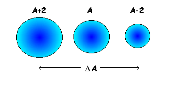
Figure 3.6: Pictorial representation of an oscillation in mass between different $L=0$ states. The macroscopic variable is the difference in mass from the initial mass partition.

The role of macroscopic variable in this game is played by the quantity $\Delta A$, that is the difference in mass from the initial mass partition. The fundamental idea of the macroscopic model for the inelastic excitations is to interpret the superposition of particle-hole excitations as representing a state of collective motion in which the systems deviates from its spherical equilibrium shape. In that case, as an alternative to the (more correct) microscopic description based on a superposition of particle-hole excitations, one has traditionally resorted to collective form factors of the form [45]

$$F_{\lambda}(r)~{}=~{}\beta_{\lambda}R{dU\over dr},$$ (3.26)

in terms of the radial variation of the ion-ion optical potential U induced by the surface vibrations, with the strength parameter $\beta_{\lambda}$ obtained from the strength of the B(E$\lambda$) transition. To generalize these concepts to the pair transfer processes we need to fulfill a number of important requirements. A couple of generalized particle-particle transition densities must be introduced to deal with addition and removal reactions ($\delta\rho^{+}_{P}$ and $\delta\rho^{-}_{P}$). An interpretation of these in terms of operator with a one-body character should be given in order to be effective.

In the case of the pair transfer, the vibration is the fluctuation of the Fermi surface with respect to the change in the number A of particles, and the corresponding form factor $F_{P}$ is assumed to have the parallel form [38]

$$F_{P}(r)~{}=~{}\beta_{P}{dU\over dA},$$ (3.27)

in terms of the “pairing deformation” parameter $\beta_{P}$ pairing deformation associated with that particular transition, defined in the previous section. The assumption of simple scaling law between nuclear radius R and mass number A allows to rewrite the two-particle transfer form factor into an expression which is formally equivalent to the one for inelastic excitation, namely

$$F_{P}(r)~{}=~{}{\beta_{P}\over 3A}~{}R~{}{dU\over dr}.$$ (3.28)

This formalism has been successfully applied to quite a number of two-particle transfer reactions [46, 47]. As in the case of inelastic excitations, macroscopic collective form-factors may in some cases only give a rough estimate to the data, requiring more elaborate microscopic descriptions. Nonetheless, the use of simple macroscopic form factors is of unquestionable usefulness in making predictions, in particular in cases, as the one we are discussing, where experimental data are not yet available and estimates are needed in order to plan future experiments.

3.4 Applications: estimates of two-neutron
transfer cross sections.

In order to evidence the possible role of unstable beams in the study of high-lying pairing states, we compare in this section two-particle transfer reactions induced either by a traditionally available beam (e.g. the (¹⁴C, ¹²C)) or by a more exotic beam (e.g. the reaction (⁶He, ⁴He)). As a target, we have considered the two cases of ²⁰⁸Pb and ¹¹⁶Sn, as representative cases of normal and superfluid systems in the pairing channels. ¹⁴C⁶He ²⁰⁸Pb¹¹⁶Sn A typical reaction scheme is shown in fig. 3.7 where in a pictorial way the phenomenon is illustrated. During the process the neutrons are transferred from the projectile to neutron single-particle states of the target, leaving an $\alpha$ particle (or ${}^{12}C$) in the exit channel. matching factor

Figure 3.7: Scheme of the two neutron transfer reaction (⁶He,⁴He). The neutrons are transferred to single-particle orbits of the target.

For the semiclassical description to be valid, the Sommerfeld parameter needs to be larger tan unity. This is certainly the case here where the product of the charges of the colliding nuclei are big and the c.m. energy is around the Coulomb barrier. In this case the transfer cross-section may be factorized in the product of the scattering cross-section, of the transfer probability and of a quantal correction factor. This correction factor, or matching factor, is important whenever the orbits of the initial and final systems (or the donor and acceptor, in the case of a transfer process) have differences in the variables that characterize the scattering orbit [48, 49, 34]. The matching factor may be written in the following way

$$F(Q,L)~{}=~{}exp\bigl{[}-c_{1}^{2}(\Delta Q-c_{2}\Delta L)\bigr{]}$$ (3.29)

where the energy matching condition and the tranferred momentum matching condition are taken into account via $\Delta Q$ and $\Delta L$, respectively. Since here we are dealing with transitions between monopole states the transferred angular momentum is zero, $\Delta L~{}=~{}0$, and thus the highest transition cross-section will be obtained if the quantal correction factor is the higest possible (equal to unity) and therefore the optimum Q-value for this kind of process is $\Delta Q~{}=~{}0$.

In both cases, we have considered the full pairing L=0 response, e.g. all transitions to 0⁺ states in ²¹⁰Pb and ¹¹⁸Sn, as described in Sect 2. The Q-values corresponding to the transitions to the ground-states and to the GPV states are displayed in Table 3.2.

	${}^{14}\mbox{C}\rightarrow~{}^{12}\mbox{C}$	${}^{6}\mbox{He}\rightarrow^{4}\mbox{He}$
${}^{116}\mbox{Sn}\rightarrow~{}^{118}\mbox{Sn}_{gs}$	3.15 MeV	15.298 MeV
${}^{208}\mbox{Pb}\rightarrow~{}^{210}\mbox{Pb}_{gs}$	-4 MeV	8.148 MeV
${}^{116}\mbox{Sn}\rightarrow~{}^{118}\mbox{Sn}_{GPV}$	-6.746 MeV	5.402 MeV
${}^{208}\mbox{Pb}\rightarrow~{}^{210}\mbox{Pb}_{GPV}$	-15.81 MeV	-3.662 MeV

Table 3.2: Q-values for ground-state and GPV transitions. The target (column) and projectile (row) are specified.

	${}^{14}\mbox{C}\rightarrow~{}^{12}\mbox{C}$	${}^{6}\mbox{He}\rightarrow^{4}\mbox{He}$
${}^{116}\mbox{Sn}\rightarrow~{}^{118}\mbox{Sn}_{gs}$	19.4 mb	0.4 mb
${}^{208}\mbox{Pb}\rightarrow~{}^{210}\mbox{Pb}_{gs}$	15.3 mb	1.8 mb
${}^{116}\mbox{Sn}\rightarrow~{}^{118}\mbox{Sn}_{GPV}$	0.14 mb	2.4 mb
${}^{208}\mbox{Pb}\rightarrow~{}^{210}\mbox{Pb}_{GPV}$	0.04 mb	3.1 mb

Table 3.3: Cross-sections for ground-state and GPV transitions obtained with the DWBA code Ptolemy. The target (column) and projectile (row) are specified.

Let us consider in greater detail the energy balance in one case for illustative purpose. The projectile and target subsystems are displayed in fig. 3.8 where the initial and final configurations are seen.

Figure 3.8: Energy balance for the two subsystems. The initial state and the final ones are displayed.

About 1 MeV is needed for the projectile to ’break’, but the lowest $0^{+}$ states of the target are some MeV higher that the ground state. The remaining energy needed is subtracted from the relative motion kinetic energy. The total energy balance is depicted in the following figure 3.9 for completeness. We have taken as an example a lead target but the same considerations apply to tin or other targets, but with different Q-values as we discussed in the tables above. Fig. 3.9 makes immediately clear that in the case of a conventional (well bound) projectile, the initial bound state would lie at much lower energy thus demanding for a greater energy to release its neutrons.

Figure 3.9: Total energy balance for the complete system. The kinetic energy borrowed from the relative motion is shown as a green arrow while the projectile and the target states are in blue and red.

For each considered state the two-particle transfer cross section has been calculated on the basis of the DWBA (using the code Ptolemy [50]) DWBA RPA employing the macroscopic form factor described above, with a strength parameter as resulting from the RPA calculation. For the ion-ion optical potential, the standard parameterization of Akyuz-Winther [51] has been used for the real part, with an imaginary part with the same geometry and half its strength. In all cases, the bombarding energy has been chosen in order to correspond, in the center of mass frame, to about 50% over the Coulomb barrier.

Figure 3.10: Differential cross-sections as a function of the excitation energy for the two reactions : a) ²⁰⁸Pb(⁶He,⁴He)²¹⁰Pb, and b) ²⁰⁸Pb(¹⁴C,¹²C)²¹⁰Pb. See text for details.

The angle-integrated L=0 excitation function is shown in Fig. 3b as a function of the excitation energy E_x for the ²⁰⁸Pb(¹⁴C,¹²C)²¹⁰Pb reaction at E_cm=95 MeV. For a more realistic display of the results, the contribution of each discrete RPA state is distributed over a lorentzian with $\Gamma$= k E${}_{x}^{2}$, with $k$ adjusted to yield a width of $4MeV$ for the giant pairing vibration. This could seem rather arbitrary since there is no reason for an a priori assignment of this quantity. We have been brought to this simple prescription because other collective states (of different nature) lying in the same energy region display similar values for their width, and it is reasonable to assume some rule to narrow the low-energy states and to broaden the high-energy ones.

As the figure shows, the large (negative) Q-value associated with the region of the GPV (see Table 1) completely damps its contribution, and the excitation function is completely dominated by the transition to the ground state and the other low-lying states. The situation is very different for the ²⁰⁸Pb(⁶He,⁴He)²¹⁰Pb reaction at E_cm=41 MeV, whose excitation function is shown in Fig. 3a. In this case the weak binding nature of ⁶He projectile leads to a mismatched (positive) Q-value for the ground-state transition (Q_gs= 8.148 MeV), favouring the transfer process to the high-lying part of the pairing response. In this case the figure shows that, in spite of a smaller pairing matrix element, the transition to the GPV is of the same order of magnitude of the ground-state transfer (1.8 mb for g.s. and 3.1 mb for the GPV). Note that a total cross section to the GPV region of the order of some millibarn should be accessible with the new large-scale particle-gamma detection systems.

Figure 3.11: Differential cross-sections as a function of the excitation energy for the two reactions : a) ¹¹⁶Sn(⁶He,⁴He)¹¹⁸Sn, and b) ¹¹⁶Sn(¹⁴C,¹²C)¹¹⁸Sn. The comparison between the GPV and the ground-state clearly shows the different strength. Notice the different vertical scale with respect to figure 3.

A similar behaviour is obtained in the case of a tin target. In Figs. 4a and 4b the corresponding excitation functions for the ¹¹⁶Sn(¹⁴C,¹²C)¹¹⁸Sn reaction (at E_cm=69 MeV) and the ¹¹⁶Sn(⁶He,⁴He)¹¹⁸Sn reaction (at E_cm=40 MeV) are compared. Now the transition to the GPV dominates over the ground-state transition when using an He beam ( 0.4 mb for g.s. and 2.4 mb for the GPV). From a comparison with the RPA strength distributions of Fig. 1 and 2 one can see that the giant pairing vibrations is definitely favoured by the use of an ⁶He beam instead of the more conventional ¹⁴C one, because the transition to the ground-state is hindered, while the GPV is enhanced (or not changed), because of the effect of the Q-value.

3.5 Conclusions.

⁶He The role of radioactive ion beams for studying different features of the pairing degree of freedom via two-particle transfer reactions is underlined. A ⁶He beam may allow an experimental study of high-lying collective pairing states, that have been theoretically predicted, but never seen in measured spectra, because of previously unfavourable matching conditions. The modification in the reaction Q-value, when passing from ¹⁴C to ⁶He, that is a direct consequence of the weak-binding nature of the latter neutron-rich nucleus, is the reason of the enhancement of the transition to the giant pairing vibration with respect to the ground-state.

The final achievements for the four reactions studied in detail are presented in the last two figures. It is worthwhile noticing that in the case of Pb there is a considerable gain in using unstable beams, while in Sn is much less evident. One sees the need for unstable helium when compares the magnitude for the pairing resonance in the right a) and b) panels with the peak at zero energy: in the first panel the transition to the ground state is extremely hindered.

A ⁶He beam is currently available (or it will be available in the very near future) in many radioactive ion beams facilities around the world and the calculations that we have presented could allow a planning for future experiments aimed to study the not yet completely unraveled role of pairing interaction in common nuclei, using exotic weakly bound nuclei as useful tools.

Projectiles with neutron excess display favourable conditions for multi-pair transfer because of their large radial extensions. Since large neutron excess is usually connected with a low binding energy Q-value considerations indicates that these reactions are suitable to populate states at higher energy, thus exciting high lying pairing vibrations. The Q-value for the reaction ${}^{206}Pb(^{8}He,^{4}He)^{210}Pb$, for example, is around $+20$ MeV, which gives optimal conditions to populate the GPV.

Chapter 4 Extension of the Steinwedel-Jensen model

4.1 Introduction

The most important role played by exotic nuclei is to force the nuclear scientific community to test its ideas within the borders of a broader new realm. We have thus discovered that the extrapolations of the theories that are working pretty well inside the stability valley may fail as long as nuclei with a large asymmetry are taken into consideration and a number of truly new phenomena arises in this region of the nuclear chart. At the driplines the presence of halos and neutron skins and the effects of the pairing interaction are believed to increase their importance, modifying many observables. This is also true for collective features and especially for the Isovector Giant Dipole Resonance (GDR). This collective mode represents the most important feature of the continuum and is very often considered an important point for the full understanding of the structure of nuclei. Work in this direction has been pursued for example by Van Isacker and collaborators [55], who studied the effect of a neutron skin on the excitation of E1 and M1 collective states by means of en extension of the Goldhaber-Teller model, finding a lowering of the average energy of these modes that they estimate to be about 5% and a fragmentation of strength. Microscopic HF+RPA calculations had shown that the value of the centroid of the energy distributions in neutron-rich nuclei is invariably smaller than the corresponding value in normal nuclei [56, 88]. Lipparini and Stringari [57], instead, had modified the Steinwedel-Jensen model to include surface effects and interaction current terms constructing an energy functional to derive the symmetry energy and polarizability as well as sum rules. Their model is nevertheless rather complicated and we will propose a simpler alternative to take into account surface effects in a straightforward way. A preliminary discussion of some of these topics may be found in [63].

Migdal [58] was the first to derive a simple power law for the dependence of the energy of the giant dipole resonance upon the atomic mass $A$. The proposed formula was $24A^{-1/3}(a_{s}Z/A)^{1/2}~{}MeV$, where $a_{s}$ is the coefficient of the symmetry term of the Bethe-Weizsäcker mass formula. Goldhaber-Teller Goldhaber and Teller (GT) [4] assumed the oscillation of a rigid proton sphere against a rigid neutron sphere with sharp surfaces, ending in a dependence of the type $A^{-1/6}$. We refer to the following section for a brief discussion. Shortly afterwards Steinwedel and Jensen (SJ) [5], developing another idea proposed in the cited work of Goldhaber and Teller, derived a formula for the oscillation Steinwedel-Jensen of proton and neutron liquids inside a common fixed spherical boundary. Their model, also called hydrodynamic or acoustical, gave the prediction $A^{-1/3}$. All these models were thought to be promising in the early stage of the study of nuclear collective phenomena, but with the growing amount of experiments on various atomic species they were negatively tested on many data [59], and it was found that a good description of the general trend is achieved with a dependence of $A^{-0.23}$. We should mention that another model, called the droplet model, has been developed [60]. It encompasses the basic assumptions of the two models and, although the physical interpretations of the two approaches remain incompatible to a large extent, it gives accurate predictions, reproducing the empirical power law.

Even if all these models are very well accepted, we felt that it was worthwhile looking at this problem with a simple model that nevertheless is capable to go beyond the actual approaches including surface effects.

The purposes of the present chapter are:

• to review and comment the predictions of some well-known models about the energy of the GDR when one moves from the prescription of $N=Z$ nuclei, showing their different trends.

• to set up a new class of models based on the extension of the Steinwedel-Jensen model with the aim of describing situations in which the nuclear surface is not sharp. In this class of models the density distribution is assumed to be of Fermi type and the region around the surface is divided in $n$ slices or steps where the density is taken to be constant. This case turns out to be solvable. When $n$ is sufficiently large the smooth function is approximated pretty well.

• to analyze the outcomings of this new class of models, namely to study qualitatively the dependence upon the diffuseness of the nuclear surface and upon the presence of a skin, showing that they predict sizable decrements in the energy of the GDR even at the level of $N=Z$ nuclei and that this is especially effective at the dripline.

The diffuse surface may reduce the energy of the mode to a large extent (up to 20%). The presence of the skin also decreases the energy of the modes, but is effective only as long as the diffuseness is kept small. When the diffuseness is taken into account the effect of the skin is not bigger than a 10%.

4.2 GT and SJ models at the driplines

Goldhaber-Teller The Goldhaber-Teller model predicts the energy of the giant resonance to be (see [62] for a detailed and simple derivation)

$$\hbar\omega~{}=~{}\hbar\sqrt{3a_{s}\over 4\epsilon m}\sqrt{A^{2}\over ZNR}\simeq{45MeV\over A^{1/6}}$$ (4.1)

where $R=r_{0}A^{1/3}$, $a_{s}$ is the asymmetry energy, $m$ is the mass of a nucleon and $\epsilon$ is a somewhat arbitrary parameter that is fixed to be $2~{}fm$. Since the two spheres are displaced the energy required is linear in the separation distance. This is certainly a bad approximation for very small separations where the symmetry energy must have a quadratic dependence. Goldhaber and Teller assumed a quadratic dependence at small separations fitted to join the linear dependence at some fixed point $\epsilon$. It is worthwhile to notice that the formula is usually approximated to its second form (valid only at $Z=N$) and that very often the coefficient is fitted from the data and taken to be $33MeV$. We have preferred to use a common value for $a_{s}$ to give a purely theoretical prediction.

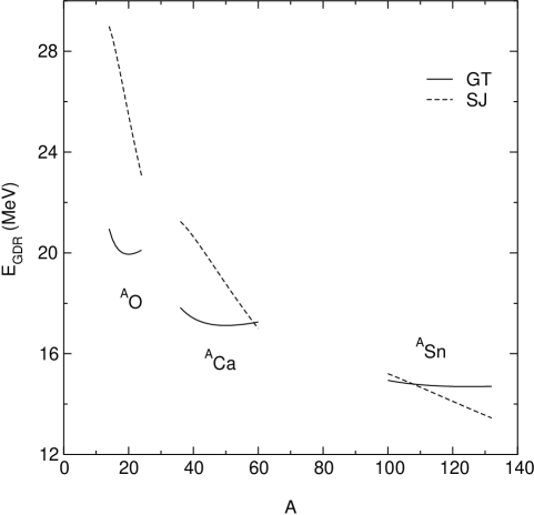
Figure 4.1: Comparison of predictions of Goldhaber-Teller (solid) and Steinwedel-Jensen (dashed) models (considering the full formulae with $a_{s}=20MeV$) for the energy of the GDR for three isotopic chains (oxygen, calcium and tin).

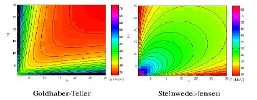
Figure 4.2: Comparison of predictions of Goldhaber-Teller (left) and Steinwedel-Jensen (right) models (considering the full formulae with $a_{s}=20MeV$) in the $(N,Z)$ plane. This is figure is due to S.Montagnani [63] (pay attention to the slightly different colouring scheme).

Steinwedel-Jensen The hydrodynamical or acoustical model of Steinwedel and Jensen takes a step function as a parameterization of nuclear densities

$$\rho_{n,p}(r)~{}=~{}\left\{\begin{array}[]{cc}\rho_{p,n}^{0}&~{}\mbox{if}~{}r\leq R_{p,n}\\ {}\hfil&{}\hfil\\ 0&~{}\mbox{if}~{}r>R_{p,n}\end{array}\right.$$ (4.2)

where the radii $R_{n,p}$ of the two distributions and the densities of the internal region, $\rho_{p,n}^{0}$, are taken as constants. This is a very crude approximation. The derivation of the energy is quite straightforward [62] and leads to the following expression

$$\hbar\omega~{}=~{}\hbar\sqrt{8a_{s}ZN\over mA^{2}}{z_{1}\over r_{0}A^{1/3}}\simeq\sqrt{4ZN\over A^{2}}{76.5MeV\over A^{1/3}}$$ (4.3)

where $z_{1}=2.08$ is the first zero of the derivative of the spherical Bessel function with $\ell~{}=~{}1$.

The second formula must be analyzed: usually one takes only the second factor because the square root reduces to 1 when $N=Z$. The remaining part agrees to a good extent with old data.

We notice however that the two formulae derived above lead to very different results when one extrapolates to the driplines. This is especially relevant nowadays since exotic beams are available and large sets of data are expected from future experiment.

In fig. 4.1 we display a comparison between the full behaviour of the GT and SJ models for three chains of different isotopes: oxygen, calcium and tin. The change of the number of neutron (and total mass) is responsible for the very different slope predicted by the two models. The differences are impressive not only for the general trends but also for the magnitude of the energy of the isovector giant dipole mode (30$\%$ in the worst case). In fig. 4.2, for each point in the $(N,Z)$ plane, the corresponding energy of the Giant Dipole Resonance is shown using different colours for different magnitudes. The opposite behaviour of GT and SJ models is clearly seen either for stable and unstable nuclei: not only the predictions along the diagonals are different in magnitudes, but also the surfaces display different curvatures while moving toward regions with excess of one of the two type of nucleons (borders of the square).

4.3 The extension of the SJ model

The nuclear surface is not sharp. It is diffuse and the Fermi distribution is known to be an efficient way to parameterize the nuclear proton and neutron densities:

$$\rho_{t}(r)~{}=~{}{\rho_{t}^{0}\over 1+e^{(r-R_{t})/a_{t}}}$$ (4.4)

where $t={n,p}$ is an index that indicates neutrons or protons respectively, $R_{t}$ and $a_{t}$ are the radius and diffuseness of the density distributions of neutrons and protons, while the saturation values are $\rho_{t}^{0}$. One may wonder that the effect of the diffuseness should be small for light nuclei and even negligible in the case of heavy nuclei. Our aim is to show in a qualitative way that it is indeed very effective in changing the predicted energy of the GDR within the Steinwedel-Jensen model, already at the level of $N=Z$ nuclei. We define the total density distribution has the sum of the density of the two species:

$$\rho_{0}(r)~{}=~{}\sum_{t}\rho_{t}(r)$$ (4.5)

It is worthwhile to insist here on the fact that every well-behaved distribution is equally treatable with the method that we are going to explain. We have decided to deal with the Fermi distribution because the degree of approximation that it furnishes is very good.

We now give a criterion to create a subdivision of the interval over which the density distribution is defined with the purpose to approximate it with a step function. The procedure that we adopt consists of the following points:

• We choose a convenient number $n$ of steps that we wish to use as an approximation. Performing the calculations a number of times with increasing $n$, we will show that the value of the energy of the giant dipole mode will converge to a finite constant value.

• We define a region around the surface in such a way that the point at which the density is one half of the value found at $r=0$ is taken as the ’center’ of the surface and we take a spherical crust whose thickness is such that the external radius always is a percentage of the inner density (10% or 5% will be taken for simplicity).

• The surface region is then divided in $n$ equally spaced intervals, and in each interval is taken a constant average density. This is also done in the case of the inner interval. In this way we have defined a step function that is an approximation to our original density distribution. We have $r_{0}$ in the origin, $n$ radii $r_{j}$, with $j=1,n$, that divide two adjacent internal intervals and finally the external radius $r_{n+1}$.

Now we have delineated a way to split the density distribution in a number of intervals. Depending on the number of intervals the outcoming model will be called a n-steps SJ model. Obviously the 0-step SJ model reduces exactly to the SJ model when the parameters $R_{t}$ and $a_{t}$ of the two distributions are equal.

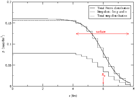
Figure 4.3: Fermi distribution function (solid line) and 10-steps SJ distribution function (dashed for n or p and dot-dashed for their sum). The radii $r_{j}$ correspond to the jumps of the step function. When the number of partitions in $r$ is increased, the approximation of the step function to the Fermi distribution becomes more effective.

We consider a continuous distribution replacing the number of particles $(N,Z)$ of each subdivision with the constant density in that interval. A plot of a typical Fermi distribution with the 10-steps function is displayed in fig. 4.3 to illustrate the way in which we approximate the density profile and the subdivision of the surface region. The higher is the number of intervals that we choose, the better is the approximation of the Fermi distribution. Thus in the limit $n\rightarrow\infty$ the step function tends exactly to the Fermi distribution (cut at some external radius). The fact that we are cutting the distribution, whose tail extends to infinity, at a given point may introduce problems. In fact whenever we increase the external radius the value of the energy decrease. To fix the ideas and to give a qualitative trend we have to make a reasonable recipe, defining the surface thickness as the region where the density drops from 90% to 10% of the inner value. This is a common prescription [61] when one is dealing with a Fermi type parameterization of the nuclear surface.

Since the magnitude of the effect depends on the way in which one cuts the distribution we have repeated these calculation several times, adopting different strategies and finding always a qualitative agreement in the results.

Insofar we have always made a distinction between neutrons and protons for the sake of generalization, but, since the two distributions may have different parameters $R$ and $a$, the resulting step functions may differ in the set of ${r_{j}}$’s. To simplify our model we take as a guide the distribution whose saturation density is higher and we derive only one set of intervals. In each interval the two distributions of protons and neutrons are defined accordingly to the average value between the two extremes of the interval. This is expected to bear no consequence on the final results, especially when the number of steps is made big.

Now we introduce, as a straightforward generalization of the Steinwedel-Jensen model, a system of $n+1$ space and time dependent equations that describes the variations of the nuclear densities, ${\rho_{t}}^{(j)}(\vec{r},t)$, within each interval as small density oscillations, $\varepsilon^{(j)}(\vec{r},t)$, of proton fluid against neutron fluid with total fixed densities ${\rho^{0}_{t}}^{(j)}$:

$${\rho_{t}}^{(j)}(\vec{r},t)~{}=~{}{\rho^{0}_{t}}^{(j)}\pm\varepsilon^{(j)}(\vec{r},t)~{}~{},\forall j=0,\cdots,n-1$$ (4.6)

where plus and minus signs refer to the two different isotopic species. Clearly in every interval the density fluctuation $\varepsilon$ of protons is opposite to the density fluctuation of neutrons. Furthermore one may think to more complex fluctuations that involve the exchange of material across different intervals. This is also included in our model because the requirement of constant total densities implies that all the fluctuations change accordingly to this request. The conservation of each kind of ’particles’ in each interval is assured by the fact that the volume integral of $\varepsilon$ is zero.

In each interval we calculate kinetic and potential symmetry energies in the standard way (see for example [62]):

$$T~{}=~{}{m\over 2}\int d^{3}r~{}\bigl{(}\rho_{p}^{(j)}{{\bf v}^{(j)}_{p}}^{2}+\rho_{n}^{(j)}{{\bf v}^{(j)}_{n}}^{2}\bigr{)}~{}=~{}$$

$${m\over 2}\int d^{3}r~{}\bigl{(}\rho_{0}^{(j)}{{\bf V}^{(j)}}^{2}+\rho_{red}^{(j)}{{\bf v}^{(j)}}^{2}\bigr{)}$$ (4.7)

where ${{\bf v}_{p,n}({\bf r},t)}^{(j)}$ are the flow velocities of protons and neutrons fluids in each interval. Transforming to relative and center of mass velocities leads to the second formula, where the first term may be eliminated requiring that the nucleus as a whole would remain at rest (${\bf V}^{(j)}=0$, $\forall j$) and where the reduced density in the $j-$th interval is given by

$$\rho_{red}^{(j)}~{}=~{}{{\rho_{p}^{0}}^{(j)}{\rho_{n}^{0}}^{(j)}\over{\rho_{0}}^{(j)}}+{{\rho_{p}^{0}}^{(j)}-{\rho_{n}^{0}}^{(j)}\over{\rho_{0}}^{(j)}}{\varepsilon^{(j)}}-{{\varepsilon^{(j)}}^{2}\over\rho_{0}^{(j)}}.$$ (4.8)

In the following only the first term will be kept. The potential energy reads instead

$$V~{}=~{}{4a_{s}\over{\rho_{0}}^{(j)}}\int d^{3}r~{}{\varepsilon^{(j)}}^{2}$$ (4.9)

The variation of the lagrangian $L=T-V$, under the assumption of hydrodynamical irrotational flow ($\nabla\times v=0$), reads

$$\delta\int dtL~{}=~{}0~{}=~{}$$

$$~{}=~{}\int dt\int d^{3}r\Biggl{(}{m\over 2}{{\rho_{p}^{0}}^{(j)}{\rho_{n}^{0}}^{(j)}\over{\rho_{0}}^{(j)}}{{\bf v}^{(j)}}^{2}-{4a_{s}\over{\rho_{0}}^{(j)}}{\varepsilon^{(j)}}^{2}\Biggr{)}$$ (4.10)

Defining the velocity and its variation as a function of the displacements, exploiting the continuity equation (at zero order in $\varepsilon$) and integrating by parts where necessary, we come up to a system of coupled differential equations for the displacements of the following form (see [62] for details, p. 200):

$$\left\{\begin{array}[]{ccc}{1\over u_{0}^{2}}{\partial^{2}\varepsilon^{(0)}\over\partial t^{2}}&~{}={}&\nabla^{2}\varepsilon^{(0)}\\ \cdots&~{}={}&\cdots\\ {1\over u_{j}^{2}}{\partial^{2}\varepsilon^{(j)}\over\partial t^{2}}&~{}={}&\nabla^{2}\varepsilon^{(j)}\\ \cdots&~{}={}&\cdots\end{array}\right.$$ (4.11)

where we have used the continuity equation at each border within different intervals and the propagation speed of density waves $u_{j}$ inside each interval is given by

$$u_{j}~{}=~{}\sqrt{8a_{s}{\rho_{n}^{0}}^{(j)}{\rho_{p}^{0}}^{(j)}\over m({\rho_{n}^{0}}^{(j)}+{\rho_{p}^{0}}^{(j)})^{2}}$$ (4.12)

The solution of the system of wave equations (4.11) gives in general a system of coupled equations of linear combinations of spherical Bessel $j(z)$ and Neumann $n(z)$ functions with $\ell~{}=~{}1$ and proper coefficients that we write as:

$$y_{j}(x,r)\equiv\alpha_{j}j(k_{j}r)+\beta_{j}n(k_{j}r)$$ (4.13)

with $k_{0}\equiv x$ and hence $k_{j}~{}=~{}u_{0}k_{0}/u_{j}~{}=~{}u_{0}x/u_{j}$, $\forall j~{}=~{}0,\cdots,n-1$. This last equivalence follows from the fact that the wavevectors $k_{j}$ are related by

$$k_{0}u_{0}~{}=~{}k_{1}u_{1}~{}=~{}\cdots~{}=~{}k_{j}u_{j}~{}=~{}\cdots$$ (4.14)

Using the definitions (4.12) we may choose only one independent $k_{j}$, that is the final goal of the solution of the system, since the energy of the Giant Dipole Resonance is $E_{GDR}~{}=~{}\hbar k_{j}u_{j}$. The solution in the innermost interval contains only the function that is regular in the origin (i.e. $\beta_{0}~{}=~{}0$), while in all the other intervals they are both present. The solutions in two adjacent intervals must connect up, together with their derivatives, and the solution in the outermost sector must have a null derivative at the outer radius $r_{0}$. No condition is explicitly required for the value of the solution at the outer radius. All these conditions set up a system of $2n+1$ equations in $2n+2$ variables

$$\left\{\begin{array}[]{cc}\left.\begin{array}[]{c}y_{0}^{\prime}(x,r)\mid_{r_{n+1}}~{}=~{}0\\ \end{array}\right\}&at~{}~{}~{}r_{n+1}\\ \cdots\\ \left.\begin{array}[]{c}y_{j+1}(x,r)\mid_{r_{j}}~{}=~{}y_{j}(x,r)\mid_{r_{j}}\\ y_{j+1}^{\prime}(x,r)\mid_{r_{j}}~{}=~{}y_{j}^{\prime}(x,r)\mid_{r_{j}}\\ \end{array}\right\}&at~{}~{}~{}r_{j}\\ \end{array}\right.$$ (4.15)

where $j=1,\cdots,n$. The system above may be easily solved: given the coefficients in the innermost interval ($\beta_{0}=0$ and $\alpha_{0}$ arbitrary, may be fixed by normalization, but this is not relevant for the present purpose), one may express the coefficients in the $j-$th interval by recursion:

$$\left\{\begin{array}[]{c}\beta_{j}~{}=~{}{{y^{\prime}_{j-1}(r)j(k_{j}r)/k_{j}-y_{j-1}(r)j^{\prime}(k_{j}r)}\over{n^{\prime}(k_{j}r)j(k_{j}r)-n(k_{j}r)j^{\prime}(k_{j}r)}}\\ {}{}{}\hfil\\ \alpha_{j}~{}=~{}{y_{j-1}(r)-\beta_{j}n(k_{j}r)\over j(k_{j}r)}\\ \end{array}\right.$$ (4.16)

The system above may be easily solved by means of a numerical FORTRAN routine by looping over the wavevector (the $(2n+2)^{th}$ variable) and looking for the point where the derivative of the solution in the outermost interval changes its sign, while crossing zero. This sets the value of the energy of the isovector giant dipole mode.

4.4 The effect of the diffuse surface

The first issue we want to discuss is the effect of the diffuseness of the nuclear surface. It is worth mentioning that whenever the diffusivity is very small the result of the calculations agrees with the Steinwedel-Jensen prediction. At all practical purposes when $a$ is $1/100$ or lower there should be no difference between the Fermi distribution and a sharp distribution.

We kept constant the saturation densities ($\rho_{p}^{0}=\rho_{n}^{0}=0.080$ nucleons/fm³) and the mass of the system ($N=Z=20$) and we studied the dependence of the energy of the giant dipole resonance on a common diffuseness parameter $a_{p}~{}=~{}a_{n}$ finding a non-negligible reduction of the energy as one can see from table 4.1.

a (fm)	$E_{GDR}$ (MeV)	%
0.0	24.23
0.01	24.13	0.4%
0.1	22.99	5.1%
0.2	21.90	9.6%
0.3	20.99	13.4%
0.4	20.21	16.6%
0.5	19.58	19.2%

Table 4.1: Energy of the giant dipole resonance as a function of the diffuseness for ⁴⁰Ca. The first value is the prediction of the Steinwedel-Jensen model, while the others are the outcome of the presently discussed model (see text). The distribution is integrated until the 10% of the inner density is reached.

The first row in this table is separated from the other because is the prediction of the pure Steinwedel-Jensen model with a rectangular distribution with the parameters given above. This calculation has a qualitative character, because we changed the radii in order to keep constant the mass of the system. The first column is the diffusivity, the second is the energy of the mode. When increasing the diffusivity we have to lower the radius of the center of the surface because, otherwise, the total mass and charge of the nucleus vary. We have thus found, for each case, the radius that maintain the total mass fixed to the original values and the effect of lowering on the energy of the giant dipole mode may amount to a lowering of about 20% with respect to the Steinwedel-Jensen prediction.

It is found, by fitting the data in this and other cases, that the dependence on the diffusivity is parabolic.

The first conclusion that one may get is that the effect of diffuseness is very strong already at the level of $N=Z$ nuclei, or along the stability valley and may be expected to be even stronger for unstable nuclei.

4.5 The effect of the skin

skin One of the most fascinating issues concerning the novel properties of very neutron- (or proton-) rich nuclei is the presence of a neutron- (or proton- ) skin. It is commonly believed, thanks to electron and hadron scattering experiments , that along the stability valley the matter distribution (radial density) of protons and neutrons have almost the same spatial extension, although different absolute value of the saturation density. That is to say the proton distribution ’follows’ the neutron distribution due to the strong pn interaction. This is certainly true for light and medium mass nuclei and partly fullfilled by heavier nuclei, but it is no more true when one moves away from stable systems.

Figure 4.4: Hartree-Fock predictions for radial density distributions of protons and neutrons in various isotopes of sulphur. The stable case (left,upper panel) has no skin while the neutron-rich isotope (right, upper panel) shows an abundance of neutron in the superficial region. The evolution of the density profiles with the number of particles is illustrated in the lower row. The vertical scales are in nucleons/fm³, while the horizontal scales are in fm.

In fact whenever the number of one of the two kinds of nucleons is by far exceeding the number of the others, many calculation and experiments indicate that the above picture is no more valid and that there is a superficial region with abundance of one of the two species. We do not attempt to resume here the extensive literature on this topic, but we refer the reader to some of the works in this field as [54, 56, 64, 65, 80, 88]. We prefer instead to present as an example the results of simple Hartree-Fock (HF) calculations with Hartree-Fock a common Skyrme type interaction to give an argument in support of the theoretical predictions of neutron skin. In fig. 4.4 a comparison between density distributions of protons and neutrons in various isotopes of sulphur is made and the corresponding differences between the neutron and proton radii are drawn in fig. 4.5. It is seen that, with this approach, a skin of a fraction of fm is envisaged even for a relatively light nucleus as sulphur. sulphur

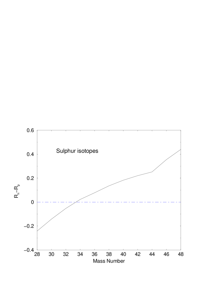
Figure 4.5: Extension of skin (in fm) versus mass number in sulphur isotopes. (HF calculations with Skyrme force). Negative values correspond to proton skins, while positive ones correspond to neutron skins.

We address now the problem of the effect of the neutron (or proton) skin on the excitation of the GDR in our schematic model increasing only one of the radii of the two distributions and keeping fixed and equal the central densities. In the following we are not interested in making accurate predictions on the real value of the energy of the Giant Dipole Mode, but we only want to discuss the effect of the presence of skin: for this reason the parameters in the table do not necessarily correspond to an integer value for the masses. We repeated these calculations with different values of the diffuseness to shed light on an interesting fact. When the diffuseness is small ($a=0.01$ fm) and the two distributions are almost box-like the effect of the skin is appreciable: the energy of the GDR drops of about 2-6 % with respect to the case with no skin as shown in table 4.2.

$R_{p}$ (fm)	$R_{n}$ (fm)	$E_{GDR}$ (MeV)
3.0	3.0	27.362
3.0	3.1	27.354	(0.03%)
3.0	3.2	26.370	(3.6%)
5.0	5.0	18.166
5.0	5.1	17.796	(2.0%)
5.0	5.2	16.914	(6.9%)

Table 4.2: Energy of the giant dipole resonance as a function of the neutron skin (difference between the two radii), having fixed $\rho_{t}^{0}=0.080$ nucl/fm³ and $a_{t}=0.1$ fm.

skin

In the same table it is also seen, by comparing the relative values of the $R=3$ fm and $R=5$ fm, that this lowering due to the skin is less effective in system with smaller masses.

$R_{p}$ (fm)	$R_{n}$ (fm)	$E_{GDR}$ (MeV)
4.0	4.0	18.621
4.0	4.1	18.393
4.0	4.2	18.119
4.0	4.3	17.541	(5.4%)
6.0	6.0	13.385
6.0	6.1	13.248
6.0	6.2	13.111
6.0	6.3	12.927	(3.4%)

Table 4.3: Energy of the giant dipole resonance as a function of the neutron skin (difference between the two radii), having fixed $\rho_{t}^{0}=0.080$ nucl/fm³ and $a_{t}=0.5$ fm.

A more appropriate value of the diffusivity ($a~{}=~{}0.5$ fm) is used in the calculations displayed in table 4.3 to understand the effect of the skin. Notice that now the value of the energies are in general smaller than in the previous case because of the effect of the diffuseness, as discussed in the previous section. In this case the additional lowering due to the presence of the skin is still sizable (3-6 %) and roughly in agreement with the estimate made in [55].

The interplay between the effect of the presence of a diffuse surface and of the skin have opposite trends in the two tables above. To understand it properly one should compare the reductions in cases where, for instance, the skin is exactly equal to one diffusivity, or to a fraction of diffusivity, and see which are the trends from light to heavy systems. This is done in table 4.4 where the densities and diffusivities are fixed and the energy of the GDR is given as a function of the radii of protons distributions for three cases: no skin (first column), skin equal to 1/5 of diffusivity (second column) and skin equal to diffusivity (third column). The third case, in which the skin has been taken unrealistically large to highlight the effect, has been supplemented with the percentage with respect to the case with no skin. It is seen that going from light systems to heavier systems, the effect of the neutron skin becomes less important.

$R_{p}(fm)$	$E_{GDR}$
	$\Delta r_{skin}/a=0$	$\Delta r_{skin}/a=1/5$	$\Delta r_{skin}/a=1$
3.0	23.13	22.81	20.66 (10.7%)
4.0	18.62	18.39	16.93 (9.1%)
5.0	15.57	15.39	14.34 (7.9%)
6.0	13.38	13.25	12.43 (7.1%)

Table 4.4: Energy of the giant dipole resonance: trends from light to heavy systems with the same ratios of skin and diffusivity ( $\rho_{p}=\rho_{n}=0.08$ nucl.$/fm^{3}$ and $a=0.5~{}fm$). It is seen how the presence of skin is less dramatic in heavier systems.

4.6 Conclusions

We have attempted a study of surface effects on the excitation of the Giant Dipole mode with the aim of shedding light on the trends associated with the presence of a diffuse surface or with the presence of a displacement of proton and neutron radii (skin). To this end we have introduced an extension of the Steinwedel-Jensen model in which the nuclear density, parameterized as a Fermi distribution, is sliced in a number of intervals and taken constant inside each interval. An exact solution of this model is proposed in terms of an iterative formula that may be easily solved.

Surprisingly we have found large reductions in the energy in connection with the presence of a diffuse surface that may even amount to the 20% of the total. In a similar way, the effect of the neutron skin has large consequences on the distribution with a very small diffusivity, but becomes less remarkable whenever a reasonable diffusivity is taken into account. This is due to the fact that situations in which the densities of the two fluids are very different tend to lower more the energy of the mode.

The study presented in this chapter is still preliminary in the sense that the prescription that we have employed to cut the distribution is arbitrary, albeit reasonable. Since the results depend on the recipe used we can only make qualitative statements: both the presence of diffuse surface and skin affects the Giant Dipole Resonance favouring a marked reduction of the energy of the mode. These findings confirm the hints that were put forward in the works of Van Isacker and collaborators, based on a modification of the Goldhaber-Teller model and in the works of Catara and others, where a microscopic description, based on RPA calcualtions, was adopted. The effects discussed here are expected to play a role in those systems far from the stability line where the presence of nuclear halos and skin are thought to be present.

Chapter 5 Break-up of dicluster nuclei

5.1 Introduction

A unique feature of nuclear systems along the neutron drip-line is the concentration of strength at excitation energies just above the continuum threshold. This concentration of strength is directly measured in breakup reactions, but it has strong effects also on other processes, such as elastic scattering or sub-barrier fusion reactions. It has been proved that this peculiar feature is associated with the weakly bound nature of most nuclei at the drip-line [64]. Within a di-cluster description of a weakly-bound nucleus (where one of the cluster may even be a single nucleon), the quantum state that describes the system lies very close to the threshold for separation into the two subsystems. The potential is in this case is the intercluster potential. The wavefunctions associated with such states (and hence their distributions of matter) extend to large radii, spreading far outside the walls of the potential well (this is valid already at the level of a square well potential, and it is even more evident for a realistic potential that has a tail at large radii). This establishes the opportunity to set a matching between the bound wave function and some scattering state in the (low-lying) continuum with approximately the same wavelength. The resulting electromagnetic response has a marked concentration of strength in the threshold region. Besides the intrinsic excitation properties of these systems, one has to consider the unusual extension of nuclear coupling on reactions, that can compete with coulomb excitation and modify inelastic form-factors and cross-sections in a sizable way [65].

The picture outlined above finds its simplest application in the case of single particle halos, where, in a mean field approach, it is the last unpaired nucleon that is responsible for the halo distribution and that, being promoted to the continuum single particle states, gives rise to the low-lying strength. The precise dipole strength distribution does not depend on the details of the binding potential, but rather on the value of the initial binding energy and on the angular momentum of the initial state, as well as on the neutron or proton character of the halo state. In all cases, however, the energy corresponding to the maximum of the strength distribution depends linearly on the binding energy [66]. Similarly, the total dipole strength at the threshold depends approximatively on the inverse of the binding energy and tends therefore to magnify its effects as one approaches the drip-lines. The picture developed so far for single-particle halos can be extended to the case of light weakly-bound nuclei within a dicluster model. We take as an ⁷Li example the case of ⁷Li, whose ground state is well described in terms of interacting $\alpha$ and triton clusters, which characterize the lowest continuum threshold (at 2.467 MeV). The basic necessary assumption is that also the excited states, both bound and unbound, are described within the same dicluster picture. In particular for the bound $1/2^{-}$ state the relative motion has been assumed to be still in the $p$ state, as the ground state, while for the continuum state the cluster-cluster relative motion can have all angular momenta. We depict in fig. 5.1 the level scheme of ⁷Li (taken from TUNL website [67]).

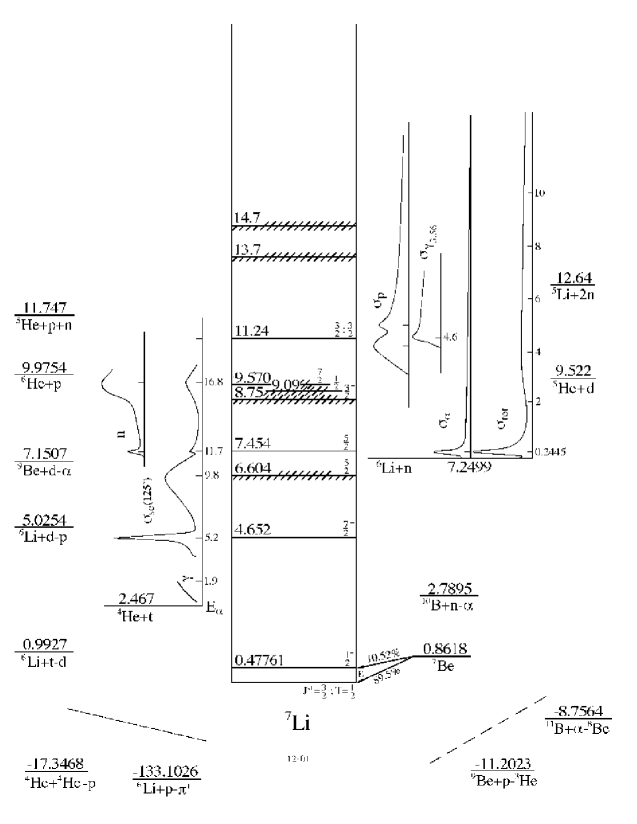
Figure 5.1: Level scheme of ⁷Li from TUNL website [67]. The data displayed here come from the compilation of Fay Ajzenberg-Selove.

The simple model for the threshold strength is modified when the system displays, in the low-energy continuum, true resonant states in addition to the non-resonant part. This is for example the case of ⁷Li which has the $7/2^{-}$ and $5/2^{-}$ states at 4.652 MeV and 6.604 MeV respectively. Within the cluster picture these states correspond to narrow resonances in the relative motion with angular momentum $\ell=3$. In a proper treatment of the continuum both resonant and non-resonant contributions arise in a natural way and may have comparable strengths. Ad hoc formalisms, which only include either the resonances or the non-resonant continuum, may therefore be inadequate to describe the full process.

A preliminary account of the concepts discussed in this article may be found in [87].

5.2 Status of dicluster systems

Figure 5.2: Wavefunctions for the ground state (solid) and first excited state (dashed) obtained solving a unidimensional Schrödinger equation for the relative motion, adjusting the depth of the Wood-Saxon potential to obtain the correct eigenvalues.

Walliser and Fliessbach [68] discuss a cluster picture for $~{}^{7}$Li, in which the constituents of the nucleus are treated as elementary, that is without internal structure, but not necessarily point-like. They obtain considerable agreement with experimental data and we conform, in principle, to their model. The main difference is that we determine the wavefunctions for the relative motion of the cluster by solving the unidimensional Schrödinger equation for an effective $\alpha-t$ potential that reads:

$$V_{\alpha-t}(r)~{}=~{}V_{coul}(r)+V_{WS}(r)+V_{\bf l\cdot s}(r)$$ (5.1)

It contains the coulomb repulsion (corrected at small distances for the sphericity of charge distributions), the nuclear Woods-Saxon attractive potential and the usual spin-orbit term [69]. By adjusting the depth of the Woods-Saxon well ($V_{WS}=-74.923$ MeV) and the magnitude of the spin-orbit correction ($V_{ls}=1.934$ MeV) we can obtain exactly the energy eigenvalues for the two bound states. The $\alpha$ cluster has spin $0$ while the $t$ cluster has spin ${1\over 2}$. The angular momentum coupling between the relative motion and the spin of the triton provides the total angular momenta $({3\over 2})^{-}$ for the ground states with energy $-2.467$ MeV and $({1\over 2})^{-}$ for the first excited state at $-1.989$ MeV [70]. The energy are measured with respect to the $\alpha-t$ break-up threshold. We give in fig. 5.2 the wavefunctions for the ground state and for the first excited state to allow a qualitative comparison with the ones obtained in the paper of Wallisser and Fliessbach (for example the radial node is at the same point). The treatment of the scattering states will be discussed later.

Quantity	This work	Experiments
$<r^{2}>_{ch}^{1/2}(fm)$	$2.44$	$2.55\pm 0.07^{(a)}$
		$2.39\pm 0.03^{(a)}$
$Q_{el}(fm^{2})$	$-3.77$	$-3.8\pm 1.1^{(a)}$
		$-3.4\pm 0.6^{(a)}$
		$-3.70\pm 0.08^{(a)}$
$Q_{mat}(fm^{2})$	$-3.99$	$-4.1\pm 0.6^{(a)}$
		$-4.00\pm 0.06^{(b)}$
$B(E2,{3\over 2}\rightarrow{1\over 2})(e^{2}fm^{4})$	$7.55$	$8.3\pm 0.6^{(a)}$
		$8.3\pm 0.5^{(a)}$
		$7.59\pm 0.12^{(b)}$
		$7.27\pm 0.12^{(b)}$
$B(M1,{3\over 2}\rightarrow{1\over 2})(\mu^{2})$	$2.45$	$2.50\pm 0.12^{(a)}$
$\Gamma({7\over 2}^{-})(keV)$	$\sim 110$	$93\pm 8^{(c)}$
$\Gamma({5\over 2}^{-})(keV)$	$\sim 930$	$875^{+200}_{-100}$

Table 5.1: Comparison of calculated and experimental quantities taken from: (a) Walliser and Fliessbach [68], (b) Voelk and Fick [71], (c) Tokimoto et al. [72]

Quantity	My work	Other works
$<r^{2}>_{ch}^{1/2}(fm)$	$2.44$	$2.43^{(a),(b)}$
		$2.55^{(c)}$
$Q_{mat}(fm^{2})$	$-3.99$	$-3.82^{(a)}$
		$-3.83^{(b)}$
		$-4.41^{(c)}$
$B(E2,{3\over 2}\rightarrow{1\over 2})(e^{2}fm^{4})$	$7.55$	$7.74^{(a)}$
		$7.75^{(a)}$
		$10.57^{(b)}$

(a) Keeley,Kemper and Rusek, PRC 60 (’02), (b) Buck and Merchant JPG 14 (’88), (c) Kajino et al., PRL 46 (’81)

We have set a simple model for $~{}^{7}$Li that nevertheless is capable of a good agreement with experimental observations, as witnessed by the list of observables in Table 1. Evaluation of charge radius, electric and matter quadrupole moments, $B(E2)$ and $B(M1)$ values for transitions between the ground state and the first excited state are reported. These quantities, except the two width, are calculated accordingly to the prescriptions given in [68]. These quantities are very sensitive to the wavefunction shape and therefore provide a reliability test for our approach as far as bound states are concerned. The two last rows in the table refer to the width of the two $f_{7/2}$ and $f_{5/2}$ resonances on which we will comment later and have been calculated with the purpose to show that this model gives also sensible predictions for the continuum states. We also compare our results with older calculations in the second table, showing that an overall agreement is found.

5.3 Electromagnetic response

electromagnetic response So far we have showed that the dicluster picture is able to give reasonable results and we would like to to apply this model to the calculations of electromagnetic response for the transitions to continuum states.

Figure 5.3: Differential B(E1) values (in $e^{2}fm^{2}/MeV$) for transitions from the ground state to the continuum. Energies are in MeV, the different contributions are indicated in the legend.

Starting from the ground state (with $p$ character) we have investigated electric dipole transitions to $s$ and $d$ states (in fig. 5.3 we give the differential reduced transition probability for dipole transitions) as well as quadrupole transitions to $p$ and $f$ states (fig. 5.4). In the former case the scattering states for even multipolarities have been calculated solving again a Schrödinger equation with the same parameters that have been used to find the bound states. The same has been done in the case of the $p$-continuum. In this scheme all the features of the transition are ascribed to the modification of the character of the angular momentum of the relative motion. The clusters are thus frozen in this picture, and their intrinsic wavefunctions are not modified by the electromagnetic operators. In the continuum energy region are present a number of resonances that deserve some further comments.

Figure 5.4: Differential B(E2) values (in $e^{2}fm^{4}/MeV$) for transitions from the ground state to the continuum. Besides there is a quadrupole transition to the first excited (bound) state, displayed in the figure as narrow peak, whose strength is indicated on the figure itself. Energies are in MeV, referred to the threshold for break-up into the $\alpha-t$ channel.

Limiting ourselves to the lowest few ones, as the ${7\over 2}^{-}$ and the ${5\over 2}^{-}$, we have solved the Schrödinger equation for scattering states with a depth of the Woods-Saxon ($V_{WS}=-68.255$) and a spin-orbit ($V_{ls}=3.115$) adjusted to yield the two resonant states in the excitation spectrum just at the right energy. Besides this resonant strength we observed a concentration of strength of non-resonant character at the separation threshold, solely due to the weakly-bound nature of the $~{}^{7}$Li nucleus. This strength is small for multipolarities that have a resonance in the low-lying continuum, but it is sizable when there are no resonances (as in the $p$ cases). The widths of these two states are in reasonable agreement with experimental observations as shown in the last part of table 1.
energy weighted sum rule energy weighted molecular
sum rule We have also compared our values with energy weighted sum rules as well as with energy weighted molecular sum rules (EWMSR) [73, 74], also called AGB sum rule from the initials of the three persons who introduced it in the literature, that are particularly useful for molecular-like structures. In light nuclei enhanced $E1$ transitions have been observed for which $B(E1)$ values may still be very small in comparison with single-particle estimates. EWMSR have been introduced as measures for these transitions and in the cases of dipole and quadrupole they read:

$$S_{I}(E1,A_{1}+A_{2})=\left({9\over 4\pi}\right){(Z_{1}A_{2}-Z_{2}A_{1})^{2}\over AA_{1}A_{2}}\left({\hbar^{2}e^{2}\over 2m}\right)$$ (5.2)

$$S_{I}(E2,A_{1}+A_{2})=\left({25\over 2\pi}\right){1\over Z}\left(Z_{1}Z_{2}+\Bigl{(}Z_{1}{A_{2}\over A}-Z_{2}{A_{1}\over A}\Bigr{)}^{2}\right)S_{0}^{2}\left({\hbar^{2}e^{2}\over 2m}\right)$$ (5.3)

where the notation means that the nucleus with mass $A$ and charge $Z$ is split in two clusters with masses $A_{1}$ and $A_{2}$, charges $Z_{1}$ and $Z_{2}$ and neutron numbers $N_{1}$ and $N_{2}$. $S_{0}$ is the equilibrium separation that may be simply calculated as the sum of the radii of the two clusters (we have taken $S_{0}=3.63$ fm). We find that our dipole strength represents approximatively the 2.6% of the Thomas-Reiche-Kuhn sum rule, but it amounts to about 94% of the energy weighted molecular dipole sum rule. Similarly the quadrupole strength is the 9.2% of the energy weigthed quadrupole sum rule and about 42% of the EWMSR. Starting from the initial ground state ($2p_{3/2}$) we have included ,in the calculation of the exhausted fraction of sum rules, all the possible transitions to lower unphysical bound states ($1s_{1/2},2s_{1/2},1d_{5/2},1d_{3/2}$ for dipole and $1p_{3/2},1p_{1/2}$ for quadrupole) and we have also included the quadrupole transition to the first excited state (see fig. 5.5 for a schematic view).

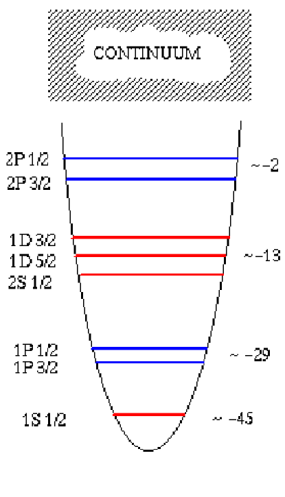
Figure 5.5: Schematic representation of the physical (2P) and unphysical (1S,1P,1D,2S) bound states and of the continuum states obtained solving the Schrödinger equation for the relative motion of the two clusters. They must be taken into account in the calculation of the energy weighted molecular sum rule. The quantum numbers of the states are on the left, while on the right is indicated their energy with respect to the threshold (in MeV).

Table 5.2: Exhausted fraction of the energy weighted sum rule and of the energy weighted molecular sum rule (AGB sum rule) for dipole and quadrupole excitation.

	E1	E2
EWSR	$2.62\%$	$\sim 9\%$
EWMSR	$94.22\%$	$\sim 42\%$

While the quadrupole transitions to bound states (both the physical $2p_{1/2}$ excited state and the two unphysical $1p$ levels) represent only a small part (about 2%) of the total quadrupole strength (that amounts to $\sim 317MeVe^{2}fm^{4}$), the total dipole strength is strongly modified: the dipole transitions to the continuum amount to $\sim 1.311MeVe^{2}fm^{2}$ and the dipole transitions to unphysical states give a negative contribution of about $\sim-0.645MeVe^{2}fm^{2}$ to the total strength. While the result for molecular dipole energy weighted sum rule is an exact one, the other is rather robust with respect to small variations in the $S_{0}$ parameter. All these values are summarized in Table 5.2

5.4 Formalism and Form Factors

We wish now to move from the electromagnetic response, that is a structural feature of ⁷Li, to the study of a breakup reaction in which the dicluster nucleus is used as a projectile on an heavy target. form factors The coordinate system for the interaction between a dicluster nucleus and a target is depicted in fig. 5.6. The factors $f_{1}$ and $f_{2}$ are the ratios of the distances of the center of mass of each cluster from the common center of mass divided by the inter-cluster distance $r$. We have named the two clusters as ’core’ and ’cluster’ to avoid confusions even if the alpha particle has not a mass so large to justify the choice with respect to triton. Nonetheless it has spin $0$ that helps in simplifying formulae.

Figure 5.6: Coordinate system for the interaction between a dicluster nucleus (white) and an external target (black).

The wavefunction for the bound initial state with angular momentum quantum numbers $J,M$ is:

$$\Psi_{JM}(\vec{r},\xi_{1},\xi_{2})~{}=~{}\sum_{\mu,m_{2}}\langle l\mu j_{2}m_{2}\mid JM\rangle\varphi_{l\mu}(\vec{r})\Phi_{1}^{j_{1}=0,m_{1}=0}(\xi_{1})\Phi_{2}^{j_{2}m_{2}}(\xi_{2})$$ (5.4)

while for the final scattering state with quantum numbers $J^{\prime},M^{\prime}$ it reads:

$$\Psi_{J^{\prime}M^{\prime}}(\vec{r},\xi_{1},\xi_{2})~{}=~{}\sum_{\mu^{\prime},m_{2}^{\prime}}\langle l^{\prime}\mu^{\prime}j_{2}^{\prime}m_{2}^{\prime}\mid J^{\prime}M^{\prime}\rangle\varphi_{l^{\prime}\mu^{\prime}}(\vec{r})\Phi_{1}^{j_{1}^{\prime}=0,m_{1}^{\prime}=0}(\xi_{1})\Phi_{2}^{j_{2}^{\prime}m_{2}^{\prime}}(\xi_{2})$$ (5.5)

where $\xi_{i}$ are the internal coordinates of the two clusters with wavefunction $\Phi_{i}$ and intrinsic quantum numbers ${j_{i},m_{i}}$. Instead $\varphi_{l^{\prime}\mu^{\prime}}(\vec{r})$ is the relative motion wavefunction, depending only on the relative coordinate. For alpha particles we have $j_{1}=0$ and $m_{1}=0$, while the triton has $j_{2}=1/2$, and hence we may simplify both formulae. The relevant interaction between the target and each component of the projectile, $V$, may be split in two parts: $V_{\alpha-T}(\mid\vec{R}-f_{2}\vec{r}\mid)+V_{t-T}(\mid\vec{R}-f_{1}\vec{r}\mid)$. Furthermore each interaction consists in a nuclear and a coulomb part. The former has a Wood-Saxon parametrization of the standard type:

$$V^{N}_{i-T}(\mid\vec{r}_{i}\mid)~{}=~{}{V_{i-T}\over 1+e^{\bigl{[}(\mid\vec{r}_{i}\mid-R_{T})/a_{i-T}\bigr{]}}}$$ (5.6)

where the index $i$ refer to one of the two clusters and the notation employed in the figure for the relative distances between each cluster and the target is shortened to $\mid\vec{r}_{i}\mid$. The Coulomb interaction takes into account the extension of the charge distributions:

$$V^{C}_{i-T}(\mid\vec{r}_{i}\mid) = \Phi_{0}{R_{T}\over\mid\vec{r}_{i}\mid},\qquad\qquad\mbox{if $\mid\vec{r}_{i}\mid>R_{T}$}$$

$$V^{C}_{i-T}(\mid\vec{r}_{i}\mid) = \Phi_{0}\Biggl{[}{3\over 2}-{\mid\vec{r}_{i}\mid^{2}\over 2R_{T}^{2}}\Biggr{]},\quad\mbox{if $\mid\vec{r}_{i}\mid<R_{T}$}$$ (5.7)

where $\Phi_{0}=Z_{eff}Z_{T}e^{2}/R_{T}$.

Figure 5.7: Form factors (in arbitrary units) for a particular transition plotted against the distance, for a fixed energy in the continuum of $E_{C}=1MeV$ (upper figure, logarithmic vertical scale) and against the energy in the continuum for three fixed distances (lower row). Coulomb (dotted) and nuclear (dashed) form factors are shown. See text for details.

The formfactor depends only on the $\vec{R}$ coordinate that is referred to the distance between the centers of mass of the two reactants and it has the form

$$F(\vec{R})~{}=~{}\langle EJ^{\prime}M^{\prime}\mid V(\vec{R})\mid JM\rangle~{}=~{}$$

$$\int d\vec{r}d\xi_{1}d\xi_{2}\Psi_{J^{\prime}M^{\prime}}^{*}(\vec{r},\xi_{1},\xi_{2})\Bigl{(}V_{1-T}(\mid\vec{r}_{1}\mid)+V_{2-T}(\mid\vec{r}_{2}\mid)\Bigr{)}\Psi_{JM}(\vec{r},\xi_{1},\xi_{2})$$ (5.8)

that can be further reduced inserting the wavefunctions above and integrating over the internal degrees of freedom. Using also some properties of the Wigner 3J and 6J coefficients and of the spherical harmonics one ends with the formula:

$$F(\vec{R})_{JMl\rightarrow J^{\prime}M^{\prime}l^{\prime}}~{}=~{}$$

$$~{}=~{}\sqrt{\pi(2J+1)(2J^{\prime}+1)}\sum_{L,\Theta}(-1)^{1/2-M^{\prime}}\Biggl{(}{J\atop-M}{J^{\prime}\atop M^{\prime}}{L\atop\Theta}\Biggr{)}\Biggl{(}{J\atop 1/2}{J^{\prime}\atop-1/2}{L\atop 0}\Biggr{)}$$

$$\Biggl{[}\int_{0}^{\infty}r_{i}^{2}dr_{i}\int_{-1}^{1}duR^{*}_{l}(r_{i})R_{l^{\prime}}V(\sqrt{R^{2}+r_{i}^{2}-2r_{i}Ru})P_{L}(u)\Biggr{]}Y_{L\Theta}(\hat{R})$$ (5.9)

where ${L,\Theta}$ are the change in orbital angular momentum and its third component due to the transition and $u$ is the cosine of the angle between the two vectors $\vec{R}$ and $\vec{r}_{i}$. Since the index $i$ is present in the square bracket there are two similar terms referring to the the two clusters. The above formula refers to a cluster with intrinsic spin quantum number $1/2$ and a more general one is provided in the appendix.

We show some results in fig. (5.7) where the Coulomb and nuclear form factors, in the same arbitrary units, are plotted for a dipole transition between the $p_{3/2,3/2}$ (second index refers to third component of angular momentum) ground state and the $s_{1/2,1/2}$ state in the continuum. From the upper panel, that shows the dependence upon $r$ when $E_{C}=1$ MeV, it is evident that the nuclear field dominates at smaller distances, while the coulomb one dominates at larger distances. This is once again displayed in the next three figures where three different distances have been kept constant and the dependence upon $E_{C}$ has been calculated. The nuclear contribution is still very important at a distance of $12-14$ fm that is far beyond the geometrical sum of the radii of the two systems. In halo systems close to the drip lines, where the wavefunctions are much more extended than in this case, this effect is even magnified. It is seen that the nuclear form factor starts to show radial nodes when the distance is increased as already noticed in [65]. Similar figures may be obtained for all the possible transitions and all display similar features.

5.5 Cross section

The formfactors obtained in the last section contain all the elements to build up elastic and inelastic cross-sections and Q-value distributions. The reaction amplitudes can be calculated in a semiclassical coupled-channel approach. semiclassical coupled channel

Figure 5.8: Q-value distribution for Coulomb breakup of ⁷Li on ¹⁶⁵Ho at $E_{cm}=40MeV$. Dipole (dotted) and quadrupole (dashed) contributions are shown together with their sum (full line). The $7/2^{-}$ resonance is marked, while the $5/2^{-}$ around 4 MeV is very small.

Figure 5.9: Differential Coulomb breakup cross sections as a function of the impact parameter with the same data of the last figure. Again different multipolarities are shown separately and one may notice the different behaviour at large impact parameter, that is dominated by the dipole contribution.

We implement here a scheme analogous to the one presented in [65], that follows a standard way of construction of elastic and inelastic cross sections [77]. For each partial wave ($\ell$) we have a set of coupled first order differential equations for the amplitudes:

$$\dot{a}_{i}^{\ell}=-i\hbar\sum F_{i,j}[\vec{R}(t)]e^{-i(\epsilon_{i}-\epsilon_{j})t/\hbar}a_{j}^{\ell}$$ (5.10)

where $\vec{R}(t)$ represents the trajectory of relative motion, while $\epsilon_{k}$ is the energy of a particular channel. The integration in time is done assuming a standard parametrization for the ion-ion potential with an imaginary part that yields a first-order elastic shift. The energy in the continuum is divided in a suitable number of intervals, treated as different channels. The reaction amplitudes obtained from this system of equations are used to calculate cross sections for the excitation of a given channel and differential cross sections as a function of the energy in the continuum. The calculations of total cross sections (as well as differential ones) must take into account the fact that one can have many choices for the initial magnetic substate (over which we must average) that are simplified since $\sigma_{p,j,m\rightarrow lj^{\prime}}=\sigma_{p,j,-m\rightarrow lj^{\prime}}$.

Figure 5.10: Q-value distribution for nuclear breakup of ⁷Li on ¹⁶⁵Ho at $E_{cm}=40MeV$. Dipole (dotted) and quadrupole (dashed) contributions are shown together with their sum (full line). The $7/2^{-}$ resonance is marked.

Fig. 5.8 is very interesting since displays the expected Q-value distribution for Coulomb breakup ( the contributions of the dipole and quadrupole transitions are separately shown, together with their sum). It is worthwhile to notice that the strength in the two peaks arise from different mechanisms: the peak at $1$ MeV is mostly build up with transition to the continuum due to the matching between initial and final wavelengths that we have already discussed, while the peak at $2.186$ MeV has a real resonant nature ($7/2^{-}$). Also in the case of quadrupole the non-resonant strength is seen just above the threshold, but its relative magnitude is small compared to the dipole one. The same informations about the relative importance of various multipolarities may be deduced from figure 5.9. In this picture one can appreciate the role of the absorption at small impact parameters, due to the implementation of a transmission factor obtained integrating the imaginary part of the potential. Moreover one can see the different behaviour of the two tails: the quadrupole contribution goes to zero in a faster way with respect to the dipole. Consequently at large impact parameters, that correspond to forward angles, the Coulomb breakup cross sections are mostly due to dipole transitions to the continuum. One can thus expect to measure dipole breakup preferably at forward angles.

Figure 5.11: Differential nuclear breakup with respect to the impact parameter.

Figure 5.12: Q-value distribution for total (interference of Coulomb and nuclear) breakup of ⁷Li on ¹⁶⁵Ho at $E_{cm}=40MeV$. Dipole (dotted) and quadrupole (dashed) contributions are shown together with their sum (full line). The $7/2^{-}$ resonance is marked.

Figure 5.13: Differential total breakup with respect to the impact parameter for the interference of Coulomb and nuclear fields.

The total Coulomb cross section at $E_{cm}=40$ MeV is around $0.48$ mb, that could be further analyzed separating the contribution of the different multipolarities: $0.20$ mb for the dipole and $0.28$ mb for the quadrupole.

The nuclear breakup at the same energy has a very similar shape for the Q-value distribution (depicted in fig. 5.11), being the total integrated cross-section about $5.78$ mb. At a variance with previous findings the dipole contribution to this cross-section ($0.14$ mb) is now much smaller that the quadrupole one ($5.64$ mb).

The comparison with fig. 5.8 shows that, while the resonances are always due to the quadrupole component, the peak at low energy is mostly due to dipole transitions for the Coulomb field and to quadrupole transitions for the nuclear field and has a different shape.

Summing up these two considerations results in a rather complicated mixing of the various components excited by the cumulative effect of the two interactions. The coulomb and nuclear cross sections have been displayed explicitly only to discuss their features. The interference of the two fields give a final Q-value distribution depicted in fig. 5.12 and a corresponding curve as a function of the impact parameter in fig. 5.13. The total cross sections in this case is about $11.9$ mb. The dipole contribution amounts to $2.5$ mb while the quadrupole is about $9.4$ mb. This result is rather large if compared with the separated Coulomb and nuclear cross sections and it is due to the interference. In order to check the validity of these estimates we have performed a simple and independent calculation with another code that evaluates Coulomb and nuclear excitation from the ground state to a sharp state (we did it for the $7/2^{-}$ resonance) given its energy and the deformation length calculated on the basis of the B(E2) value (that is the integral of the curve in figure 5.4 corresponding to the resonance). The result gives $0.34$ mb for Coulomb excitation. This number is roughly consistent with the value of the quadrupole component of the Coulomb cross section (half of which may be attributed to the resonance).

5.6 Parallel work on ⁶Li

⁶Li Besides the detailed discussion on ⁷Li a parallel investigation on ⁶Li has been carried on with the purpose of comparing the results with other theoretical predictions and experiments [78, 79]. We briefly report here on the status of this research line.

The level scheme of ⁶Li is reported in fig 5.14 for the sake of completeness. The ground state is the only bound state below the threshold for separation into an $\alpha$ particle plus a deuteron. Its binding energy is about 1.5 MeV. This makes of ⁶Li a very weakly-bound nucleus. Three resonances with $T=0$ isospin quantum number are seen in the low-lying continuum with $J^{\pi}~{}=~{}3^{+},2^{+},1^{+}$ interpreted as the coupling of the spin of the clusters with a d-wave relative motion. Resonances with $T=1$ are not included in the present analysis.

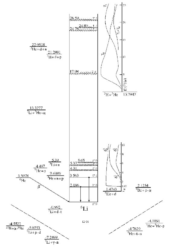
Figure 5.14: Level scheme of ⁶Li from TUNL website [67]. The data displayed here come from the compilation of Fay Ajzenberg-Selove.

The same physical idea of the description of $~{}^{6}$Li as a dicluster nucleus (alpha plus deuteron) has been retained and the Schrödinger equation has been solved for the relative motion both for the bound and the continuum states, adjusting the depth of the Saxon-Woods potential to obtain the correct binding or resonance energies. The relative motion has then been treated along a classical trajectory in a semi-classical coupled channel approach that has the advantage to be very straightforward to solve numerically and to require lower CPU times than other commonly used approaches. This allows a finer subdivision of the continuum (for example we have done the calculations with energy bins of 0.1 MeV). The results for the cross sections and excitation energy distribution, although not including continuum-continuum couplings, are very similar to the one obtained with other methods, like the continuum discretized coupled channel method. At 39 MeV bombarding energy our total breakup cross section (integrated over the continuum energy) is about 85 mb, close to the value of 104 mb obtained with CDCC procedure.
CDCC

Table 5.3: Comparison between ⁶Li breakup cross section evaluated by semi-classical calculation and CDCC, and experimental data. All cross sections are in mb. It is seen that both theories slightly overestimate the experimental values. [Data are due to the courtesy of M.Mazzocco].

Beam	Semi-classical	CDCC	Experimental
energy	calculation		data
31 MeV	54.9	48.76	41.3(0.7)
33 MeV	69.3	65.43	59.2(1.2)
35 MeV	77.9	80.91	63.0(2.6)
39 MeV	84.5	102.32	76.5(5.3)

The most important qualitative difference is the proper inclusion of non-resonant continuum states [80] that arise from the weakly-bound nature of the ⁶Li nucleus [64]. We report in fig. 5.15 the differential B(E2) values to the low-lying continuum (in the case of ⁶Li the dipole vanish identically in a cluster picture because the effective charge is zero for an alpha plus deuteron cluster configuration).

Figure 5.15: Differential B(E2) values (in $e^{2}fm^{4}/MeV$) for transitions from the ground state to the continuum for the breakup of ⁶Li. In the inset we display the full vertical scale. Energies are in MeV, referred to the threshold for break-up into the $\alpha-d$ channel.

The transitions to the non-resonant continuum are strong enough to smear the 2⁺ and 1⁺ resonances, thus introducing a slight qualitative difference between the two lineshapes. This is consistent with the trends of the data sets and a finer energy resolution would be advisable to settle the problem. Instead the 3⁺ resonance is not modified appreciably because, at a variance with the CDCC calculations, we find a narrow and strong peak. This difference may be due to the different way of subdivision of the continuum into energy bins.
As it appears from the table below, however, both approaches slightly overestimate the integrated experimental cross sections.

5.7 Conclusions

We have illustrated a general method to treat dicluster nuclei, showing how to obtain their structure features and we have implemented a semiclassical calculation to perform breakup reaction studies.
The main idea was developed in the papers by Dasso, Lenzi ans Vitturi, who showed how the non-resonant continuum affects the excitation properties and the breakup of neutron and proton halos in weakly-bound nuclei. Our aim was to extend this picture to cluster states and to show the importance of transition to low-lying continuum in weakly-bound dicluster systems.
We have not attempted a detailed comparison with other methods, but we based our arguments on the fact that the cluster description of light nuclei is widely accepted. We expect that the semiclassical implementation of a coupled channel scheme is not inferior to some, in principle more correct, fully quantistic coupled channel calculations. Our scheme is simpler and faster and allows a binning of the continuum that may be as fine as one wishes. Other methods are constrained to a rougher subdivision of the energy. Nonetheless we argue that the effects of the non-resonant strength on the final cross sections are twofold: they modify the lineshape and increase the magnitude of the cross sections in a sizable way.
This work may turn out to be relevant to studies on complete and incomplete fusion reactions: in a nuclear reaction with a weakly-bound projectile, the field of the target may act on the projectile in such a way to break it before the collision, and the breakup may be followed by fusion of both fragments, of only one of the two or of none. In this respect the effect of break-up on fusion processes is among the topics of higher current interest for the nuclear physics community.

5.8 Appendix to the chapter

We would like to give here a formula for the calculation of the form factors with the same purpose of (5.8) for a generic cluster with intrinsic spin quantum number $j_{2}$:

$$F(\vec{R})_{JMl\rightarrow J^{\prime}M^{\prime}l^{\prime}}=\sqrt{\pi(2J+1)(2J^{\prime}+1)(2\ell+1)(2\ell^{\prime}+1)}$$

$$\sum_{L,\Theta}(-1)^{3j_{2}-M^{\prime}}\Biggl{(}{\ell^{\prime}\atop 0}{\ell\atop 0}{L\atop 0}\Biggr{)}\Biggl{(}{J\atop-M}{J^{\prime}\atop M^{\prime}}{L\atop\Theta}\Biggr{)}\Biggl{\{}{J\atop\ell}{J^{\prime}\atop\ell^{\prime}}{L\atop j_{2}}\Biggr{\}}$$

$$\Biggl{[}\int_{0}^{\infty}r_{i}^{2}dr_{i}\int_{-1}^{1}duR^{*}_{l}(r_{i})R_{l^{\prime}}V(\sqrt{R^{2}+r_{i}^{2}-2r_{i}Ru})P_{L}(u)\Biggr{]}Y_{L\Theta}(\hat{R})$$

where the symbols have the same meanings of the text. The simplifications used to calculate the form factor for ⁷Li no longer apply when the cluster has not $j_{2}=1/2$.

Chapter 6 Summary and epilogue

6.1 Summary

We have tried to give a unitary exposition of the researches that we undertook during the three years of study and work in Padova, sewing together apparently different subjects, that nevertheless have a common basic goal: the understanding of collective modes and of the continuum in which these modes are usually embedded, especially in connection with novel phenomena seen in nuclei far from the stability line. We attacked this problem from many different sides taking particular care for the role of exotic nuclei either as a subject or as a tool to understand a particular issue. Not only the presence of clustering, halos and skins have been considered as ’exotic’ phenomena, affecting the properties of excitation of dripline nuclei, but also ’exotic’ (in the sense of unconventional or less frequently discussed) collective modes have been discussed, as for example the Giant Pairing Vibrations excited with unstable nuclei.

The themes covered in the present thesis are: a detailed study of double phonon giant resonances in normal nuclei, the enhancement of the excitation of Giant Pairing Vibrations using weakly-bound nuclei, an extension of the Steinwedel-Jensen model for Giant Dipole Resonances to treat surface effects and presence of neutron skin and, finally, a model on breakup reactions in weakly-bound dicluster nuclei.

The common idea underlying these four chapters, and in some way its mortar, is the interpretation of nuclear phenomena by means of collective models that have the virtue of being simple and well characterized from a physical point of view. Needless to say it has been also useful to look at the many-body problem in terms of microscopic theories, if need be. Another cementing feature of our arguing has been the profitable resort to semiclassical reaction theory, as far as reaction models were concerned.

The keystone of many problems that we had encountered was to solve ordinary differential equation or systems of ODE’s, from the Schrödinger equation in dicluster states to the equations of motion in the semiclassical theory nuclear reactions, or from the wave equation in two-fluids acoustical models to coupled channels reaction amplitudes. This task has been accomplished analitycally, when possible, or numerically, implementing throughout the whole thesis computer codes that exploit a very versatile subroutine to solve systems of first ordinary differential equations.

Epilogue

There would be no better conclusion to this thesis than to quote again the same Master that we cited at the beginning of this work, because, once again, his words are of the utmost relevance:

”He! he! he! –he! he! he! –yes, the Amontillado. But is it not getting late? Will not they be awaiting us at the palazzo, the Lady Fortunato and the rest? Let us be gone.”
”Yes,” I said, ”let us be gone.”
- The cask of Amontillado amontillado - Edgar Allan Poe.

subjectSubject Index

Bibliography

- [1] M. N. Harakeh and A. van Woude, Giant Resonances (2001 Oxford University Press, New York).
- [2] W. Bothe and W.Gentner, Z. Phys. 106 (1937) 236.
- [3] G.C.Balwin and G.Klaiber, Phys.Rev. 71 (1947) 3.
- [4] M.Goldhaber and E.Teller, Phys.Rev. 74 (1948) 1046.
- [5] H.Steinwedel and J.H.D.Jensen, Z.Nat. 52 (1950) 413.
- [6] A.Pitthan and Th.Walcher, Phys. Lett. 318 (1971) 563.
- [7] M.B.Lewis and F.E.Bertran, Nucl.Phys. A196 (1972) 337.
- [8] G.F.Bertsch and R.A.Broglia, Oscillation in finite quantum systems, (Cambridge Univerity Press, 1994).
- [9] N Frascaria, Nucl. Phys. A687 (2001) 154c-161c.
- [10] H. Hemling, Prog. Part. Nucl. Phys. 33 (1994) 729; T. Aumann, P. Bortignon, and H. Emling, Annu. Rev. Part. Sci. vol. 48 (1998) 351.
- [11] Ph. Chomaz, and N. Frascaria, Phys. Rep. 252 (1995) 275.
- [12] M.A.Kovash et al., Phys.Rev.Lett. 42 (1979) 700.
- [13] LAND collaboration, Phys.Rev.Lett. 70 (1993) 1767.
- [14] H.Emling et al., Nucl. Phys. A569 (1994) 141c
- [15] S. Nishizaki and J. Wambach, Phys. Lett. B349 (1995) 7; ibid. Phys. Rev. C57 (1998)1515.
- [16] V. Yu. Ponomarev, P. F. Bortignon, R. A. Broglia, E. Vigezzi and V. V. Voronov, Nucl. Phys. A599 (1996) 341c.
- [17] C. A. Bertulani and V. Yu. Ponomarev, Phys. Rep. 321 (1999) 139.
- [18] F. Catara, Ph. Chomaz and N. Van Giai, Phys. Lett. B233 (1989) 6.
- [19] V. Yu. Ponomarev, P. F. Bortignon, R. A. Broglia, and V. V. Voronov, Phys. Rev. Lett. 85 (2000) 1400.
- [20] E. G. Lanza, M. V. Andrés, F. Catara, Ph. Chomaz and C. Volpe, Nucl. Phys. A613 (1996) 445; ibid. Nucl. Phys. A654 (1999) 792c.
- [21] C. Volpe, F. Catara, Ph. Chomaz, M. V. Andrés and E. G. Lanza, Nucl. Phys. A589 (1995) 521; ibid.Nucl. Phys. A599 (1996) 347c.
- [22] P. F. Bortignon and C. H. Dasso, Phys. Rev. C56 (1997) 574.
- [23] D. Brink, PhD Thesis, Oxford University, 1955, unpublished; P. Axel, Phys. Rev. 126 (1962) 671.
- [24] B. V. Carlson et al., Ann. Phys. (NY) 276 (1999) 111; Phys. Rev. C60 (1999) 014604.
- [25] J. Z. Gu and H. A. Weidenmüller, Nucl. Phys. A690 (2001) 382.
- [26] F. Catara, Ph. Chomaz and A. Vitturi, Nucl. Phys. A471 (1987) 661.
- [27] E. G. Lanza, M. V. Andrés, F. Catara, Ph. Chomaz and C. Volpe, Nucl. Phys. A636 (1998) 452.
- [28] M. V. Andrés, F. Catara, E. G. Lanza, Ph. Chomaz, M. Fallot anf J. A. Scarpaci, Phys. Rev. C65 (2001) 014608.
- [29] L. F. Canto, A. Romanelli, M. S. Hussein and A. F. R. de Toledo Piza, Phys. Rev. Lett. 72 (1994) 2147.
- [30] C. A. Bertulani, L. F. Canto, M. S. Hussein and A. F. R. de Toledo Piza, Phys. Rev. C53 (1996) 334.
- [31] K. Alder and A. Winther, Electromagnetic Excitation (North-Holland, Amsterdam, 1975).
- [32] R. A. Broglia and A. Winther, Heavy Ion Reactions Vol.I (1981 The Benjamin/Cummings Publishing Company).
- [33] S. Landowne and A. Vitturi, in Treatise on Heavy Ion Science, Ed. D. A. Bromley, vol. 1, p.355.
- [34] W. von Oertzen and A. Vitturi, Rep. Prog. Phys. 64 (2001) 1247-1338
-
[35]
R.A. Broglia and D.R. Bes, Phys. Lett. B69 (1997)
129
M.W Herzog, R.J. Liotta and T Vertse, Phys. Lett. B165 (1985) 35. -
[36]
G.M. Crawley et alt., Phys. Rev. C23 (1981) 589.
W. von Oertzen and al., Z.Phys. A313 (1983) 371-372. -
[37]
A. Bohr and B.R. Mottelson, Nuclear Structure,
Vol. II, Benjamin, Reading (1975)
R.A. Broglia, O. Hansen and C. Riedel, Adv. Nucl. Phys. 6 (1973) 287. - [38] Collective Aspects in Pair Transfer Phenomena, ed. C.H. Dasso and A. Vitturi, Società Italiana di Fisica, Editrice Compositori, Bologna 1987, Vol. 18.
- [39] D.R. Bes and R.A. Broglia, Phys. Rev. C3 (1971) 2349.
- [40] M.G.Mayer and J.H.D.Jensen, Elementary Theory of Nuclear Shell Structure, Willey, New York, N.Y. (1955)
- [41] C.Dasso, private communication
- [42] J.Blomqvist and S.Wahlborn, Arkiv för Fysik 16 (1960) 545.
- [43] R.A.Uhrer and R.A.Sorensen, Nucl Phys. A86 (1966) 1.
- [44] C.H.Dasso and R.J.Liotta, Phys.Rev. C36 (1987) 448.
- [45] G.R. Satchler, Direct Nuclear Reactions, Clarendon press, Oxford 1983
- [46] C.H.Dasso and G.Pollarolo, Phys. Lett. 155B (1985) 223.
- [47] C.H.Dasso and A.Vitturi, Phys. Rev. Lett. 59 (1987) 634.
- [48] R.A.Broglia, G.Pollarolo and A.Winther, Nucl Phys. A361 (1981) 307
- [49] W.von Oertzen in Heavy Elements and Related Phenomena Vol.I, ed. R.K.Gupta and W.Greiner (1999) World Scientific (Singapore).
- [50] M.Rhoades-Brown, M.McFarlane and S.Pieper, Phys. Rev. C21 (1980) 2417; Phys. Rev. C21 (1980) 2436.
- [51] R.A.Broglia and A.Winther, Heavy Ion Reactions Vol.I (1981) The Benjamin/Cummings Publishing Company.
- [52] S.Gustavson, I.L.Lamm, B.Nilsson and S.G.Nilsson, Arkiv för Fysik 36 (1967) 613.
- [53] P.Lotti et al., Phys.Rev. C40 (1989) 1791.
-
[54]
T.Suzuki et al., Phys.Rev.Lett. 75 (1995)
3241;
I.Hamamoto et al., Phys.Rev. C52 (1995) R2326; ibid. C53 (1996) 765;ibid. C54 (1996) 2369;
S.Mizutori et al., Phys.Rev. C61 (2000) 044326;
H.Sagawa et al., Phys.Rev. C65 (2002) 064312;
S.Karataglidis et al., Phys.Rev. C65 (2002) 044306. - [55] P.Van Isacker, M.A.Nagarajan and D.D.Warner, Phys.Rev C 45 (1992) 45-49.
- [56] F.Catara et al., Nucl.Phys. A624 (1997) 449; Nucl.Phys. A614 (1997) 86;
- [57] E.Lipparini and S.Stringari, Phys.Rep. 175 (1989), issues 3-4, 103-261.
- [58] A.Migdal, J.Phys. (Moscow) 8 (1944), 331.
- [59] B.L.Berman and S.C.Fultz, Rev.Mod.Phys. 47, (1975), 713.
- [60] W.D.Myers and W.J.Swiatecki, Ann.Phys. (N.Y.) 55, (1969), 395.
- [61] G.A.Jones, Rep. Prog. Phys. 33 (1970), 645-689
- [62] W.Greiner and J.A.Maruhn, Nuclear Models, Springer (1996).
- [63] Stefano Montagnani, degree thesis, University of Padova (2002) [in italian].
- [64] C.H.Dasso, S.M.Lenzi and A.Vitturi, Nucl. Phys. A639 (1998), 635-653.
- [65] C.H.Dasso, S.M.Lenzi and A.Vitturi, Nucl. Phys. A611 (1996), 124-138.
- [66] M.A.Nagarajan, S.M.Lenzi, A.Vitturi, to be published.
- [67] http://www.tunl.duke.edu/nucldata/
- [68] H.Walliser and T.Fliessbach, Phys. Rev. C31 (1985), 2242.
- [69] A.Bohr and B.Mottelson, Nuclear Structure W.A.Benjamin, Inc.(1969) New York,Amsterdam.
- [70] D.R.Tilley et al. Nucl. Phys. A708 (2002), 3-163.
- [71] H.G.Voelk and D.Fick, Nucl. Phys. A530 (1991), 475-489.
- [72] Y.Tokimoto et al., Phys. Rev. C63 (2001), 035801.
- [73] Y.Alhassid, M.Gai and G.F.Bertsch, Phys. Rev. Lett. 49 (1982), 1482.
- [74] H.J.Assenbaum, K.Langanke and A.Weiguny, Phys. Rev. C 35 (1987), 755.
- [75] C.M.Perey and F.G.Perey, At. Data Nucl. Data Tab.17 (1976), 1.
- [76] R.P.Ward and P.R.Hayes, At. Data Nucl. Data Tab.49 (1991), 316.
- [77] R.A.Broglia and A.Winther, Heavy ion reactions (Addison-Wesley, Redwood City,1991).
- [78] C.Signorini et al., submitted.
- [79] G.R.Kelly et al., Phys. Rev. C63 (2000), 024601.
-
[80]
F.Catara,C.H.Dasso and A.Vitturi, Nucl. Phys.
A602 (1996), 181.
——————————————————————————
- [81] C.H.Dasso, L.Fortunato, E.G.Lanza and A.Vitturi, Nucl. Phys. A724 (2003), issue 1-2, 85-98.
- [82] L.Fortunato, H.M.Sofia, W.von Oertzen and A.Vitturi, Eur.J.Phys. A 14, (2002), issue 1, 37-42.
- [83] L.Fortunato, Phys. At. Nucl. (Yadernaya Fizika) 66 (2003),issue 8, 1445-1449, and Procedings of HIP02, Dubna, Russia (2002) (World Scientific).
- [84] L.Fortunato, in ”Theoretical Nuclear Physics in Italy”, Proceedings of the 9th Conference on Problems in Theoretical Nuclear Physics, S.Boffi et al. ed., (2003) (World Scientific).
- [85] L.Fortunato, S.Montagnani and A.Vitturi, in preparation.
- [86] L.Fortunato and A.Vitturi, in preparation.
- [87] L.Fortunato, Heavy Ion Physics ( Heavy Ion Phys., in press) and Proceedings of 284th Heraeus seminar, Marburg, Gemany (2002) (World Scientific). URL: http://arxiv.org/abs/nucl-th/0209013
- [88] L.Fortunato and A.Vitturi, Nucl. Phys. A722 (2003) 85c-91c and Proceedings ISPUN02 (Elsevier, 2003).
- [89] L.Fortunato and A.Vitturi, Proceedings CM2002.
- [90] C.Signorini, P.Scopel, M.Mazzocco, L.Fortunato, F.Soramel, I.J.Thompson, A.Vitturi, M.Barbui, A.Brondi, M.Cinausero, D.Fabris, E.Fioretto, G.La Rana, M.Lunardon, R.Moro, A.Ordine, G.F.Prete, V.Rizzi, L.Stroe, M.Trotta and E.Vardaci, Eur.J.Phys. accepted
Index