Shear Viscosity Coefficient from Microscopic Models

Abstract

The transport coefficient of shear viscosity is studied for a hadron matter through microscopic transport model, the Ultra–relativistic Quantum Molecular Dynamics (UrQMD), using the Green–Kubo formulas. Molecular–dynamical simulations are performed for a system of light mesons in a box with periodic boundary conditions. Starting from an initial state composed of $\pi,\,\eta\,,\omega\,,\rho\,,\phi$ with a uniform phase–space distribution, the evolution takes place through elastic collisions, production and annihilation. The system approaches a stationary state of mesons and their resonances, which is characterized by common temperature. After equilibration, thermodynamic quantities such as the energy density, particle density, and pressure are calculated. From such an equilibrated state the shear viscosity coefficient is calculated from the fluctuations of stress tensor around equilibrium using Green–Kubo relations. We do our simulations here at zero net baryon density so that the equilibration times depend on the energy density. We do not include hadron strings as degrees of freedom so as to maintain detailed balance. Hence we do not get the saturation of temperature but this leads to longer equilibration times.

I Introduction

High energy heavy ion reactions are studied experimentally and theoretically to obtain information about the properties of nuclear matter under the extreme conditions of high densities and /or temperatures. One of the most important aspects of studying nucleus-nucleus reactions at these extreme conditions is the possibility that normal nuclear matter can undergo a phase transition into a new state of matter, the quark–gluon plasma [QMreviews]. In this state the degrees of freedom are partons (quarks and gluons).

In this work we study only the the thermodynamic and transport properties of hadron matter. Hence the relevant degrees of freedom are hadrons. We study the equilibration of the system in infinite hadron matter using UrQMD [2]. We restrict ourselves to a a system that contains only meson resonance degrees of freedom. The infinite hadron matter is modelled by initializing the system by light mesons only. We fix baryon density and energy density of the system in a cubic box and impose periodic boundary conditions. We then propagate the system in time until we obtain equilibration.

The equation of state and transport coefficients of hot, dense hadron gases are quite important quantities in high energy nuclear physics. In the ultra–relativistic heavy ion experiments at CERN and BNL, the final state of interactions is dominated by hadrons and hence the observables are mainly hadrons. Therefore knowledge of the equation of state and transport coefficients of a hadron gas is necessary for a better understanding of the observables. Phenomenologically both the transport properties and the equation of state of hadron gas are the major source of uncertainties in dissipative fluid dynamics.

In spite of their importance, the equation of state and transport coefficients of hot, dense hadron gases are still poorly known because of the nonperturbative nature of the strong interaction. Progress in the study of hadron matter transport coefficients is very slow, and only a calculation of transport coefficients in the variational method [3, 4] and relaxation time approximation [5] has been done. From those previous studies a lot has been learned about the transport coefficients of binary mixtures such as $\pi\pi$ system. However in a more realistic situation we need to describe transport properties of a many–body system. This in turn would require taking into account various interaction processes and in–medium effects. Thus, we need to investigate the thermodynamic and transport properties of a hadron gas by using a microscopic model that includes realistic interactions among hadrons. In this work, we adopt a relativistic microscopic model, UrQMD and perform molecular–dynamical simulations for a hadron gas of mesons.

We focus on the hadronic scale temperature ($100$ MeV $<T<200$ MeV) and zero baryon number density which are expected to be realized in the central high energy nuclear collisions. Thermodynamic properties and transport coefficients of hadronic matter in this region should play important roles in dissipative fluid dynamical models. Sets of statistical ensembles are prepared for the system of fixed energy density and baryon number density. Using these ensembles, the equation of state is investigated. The statistical ensembles is then applied in calculating the shear viscosity coefficient of a hadron gas of mesons.

The equation of state of a hot and dense hadron gas had been investigated using UrQMD [2, 6]. The work has provided valuable information regarding the nature of the hadron gas. In those simulations the temperature reaches a limiting value with increasing energy density. This is because in those simulations the detailed balance is broken. This in turn leads to the irreversibility of the equilibrated system. And without the reversal process of multi–particle production energy balance between the forward and backward reactions is no longer realized and hence the saturation of the temperature occurs. Although it is interesting and important to formulate these multi–particle interaction processes exactly in the present simulation, straightforward implementation of them is not easy. In this work, avoiding this complicated problem, we disabled three or many–body interactions in UrQMD. We have also disabled decays or interactions that involves photons.

The rest of the paper is organized as follows: In section II we study the equilibration and thermodynamics of the system. In section III we study the thermodynamic of a pure resonance meson gas for comparison with the results from UrQMD. In section IV we calculate the shear viscosity coefficient from stress tensor fluctuations around the equilibrium state through UrQMD using Green–Kubo relations. Finally in section V we summarize our results.

II Equilibration of infinite matter in a box

To investigate the equilibration of the system we performed microscopic calculation using UrQMD. UrQMD is designed to simulate ultra–relativistic heavy ion collision experiments. The description of the model can be found in [2]. In studying the equilibration of the hadron gas we would like to maintain detailed balance in the simulations. Multi–particle productions plays an important role in the equilibration of the hadron gas. However in UrQMD their inclusion in the simulations breaks detailed balance due to the absence of reverse processes. In order to avoid this problem in the present simulations we consider only up to two–body absorption/annihilation and decay processes. Thus the fundamental processes in the UrQMD version we use here are two–body elastic and quasi-elastic collisions between hadrons, and strong decays of resonances. Even though we started with light mesons in the initial state we consider all the mesons and meson–resonance included into the UrQMD model, in the final state.

When studying the equilibration of hadron gas it is important to maintain detailed balance in the microscopic model. Though the contributions of the multi-particle productions dominate the system at early stages of the non–equilibrated system, the reverse process plays an important role in the latter, equilibration stage. The absence of reverse processes leads to one-way conversion of the energy to particles. However, the exact treatment of multi–particle absorption processes is very difficult. In order to treat them effectively in our case, we only consider up to 2-body decays.

In this work, we focus our investigation on the thermodynamic and transport properties of a hadronic system. For this purpose, we consider a system in a cubic box and impose periodic boundary conditions in configuration space. Thus if a particle leaves the box, another one with the same momentum enters from the opposite side. This calculation is similar to the one done in [6] but with different degree of freedom and included processes in the system. A further similar analysis was done in [7, 8] using different cascade models with different degrees of freedom.

The energy density $\varepsilon$ and the baryon number density $n_{B}$ in the box are fixed as input parameters, and these quantities are conserved throughout the simulation. The initial distributions of mesons are given by uniform random distributions in phase space. The energy is defined as $\varepsilon=E/V$, where $E$ is the energy of $N$ particles:

$$E=\sum_{i=1}^{N}\sqrt{m^{2}_{i}+p_{i}^{2}}$$ (1)

The 3–momenta $p_{i}$ of the particles in the initial state are randomly distributed in the center of mass system of the particles:

$$\sum_{i=1}^{N}p_{i}=0\enspace.$$ (2)

The time evolution is now described by UrQMD. Though the initial particles are only $\pi\,,\eta\,,\omega\,,\rho\,,\phi$, many mesons and meson–resonances are produced through interactions. We now propagate all particles in the box using periodic boundary conditions, that is, particles moving out of the box are reinserted at the opposite side with the same momentum. The phase–space distribution of mesons then can change due to elastic collisions, resonance production and their decays to lighter mesons again. We recall that we include all the mesons and meson–resonances in UrQMD.

To investigate the equilibration phenomena of the system we look at the particle densities and energy distributions of each particle. As time increases the system tends towards an equilibrium state. When the system is in thermal equilibrium, the slope parameters of the energy distributions for all particles should have the same value, and that value is the inverse of temperature. To investigate this, we study the time evolution of the inverse slopes of various particles.

Running UrQMD many times with the same input parameters and taking the stationary configuration in equilibrium, we can obtain statistical ensembles with fixed temperature. By using these ensembles, we can calculate thermodynamic quantities, such as the particle density, pressure, and so on, as functions of temperature and baryon number density. We extract the shear viscosity coefficient by finding the energy–momentum tensor correlations and then employ the Green–Kubo relations..

We specify the initial input parameters: the volume of the box $V$, the net baryon number density $n_{B}$, and the total energy density $\varepsilon$. We consider the input parameters which will give the temperature range 100 – 200 MeV. Here $n_{B}=0.0$ fm^-3 is taken as the net baryon number density of the system. We generated a statistical ensemble of 200 events.

A Chemical Equilibration

Figure 1 shows the time evolution of the various particles densities ($\pi,\eta,\rho,K$) at zero net baryon number density and energy density $\varepsilon=0.3$ GeV/fm³. After several fm/c the number of pions decreases first due to inelastic collisions and annihilation that produces other meson resonances. The pion density then increases due to decay of heavier meson resonances to an equilibration. The number of kaons (in general strange mesons) increases to equilibration value in much longer times than other particles. In figure 2 we show the same situation but with different initial energy density of the box, $\varepsilon=0.9$ GeV/fm³. For large initial energy densities the equilibration times are much larger.

FIG. 1.: The time evolution of particle densities for each particle with $V=1000$ fm³ and $\varepsilon=0.3$ GeV/fm³.

FIG. 2.: The time evolution of particle densities for each particle with $V=1000$ fm³ and $\varepsilon=0.9$ GeV/fm³

Figures 1 and 2 display the time evolution of particle densities. These figures show that the system approaches a stationary state with time. The saturation of particle densities indicates the realization of chemical equilibrium. We conclude that chemical equilibrium in our system is realized.

B Thermal Equilibration and Temperature

In this subsection we investigate the approach to thermal equilibrium. This is driven by the momentum equilibration of the system. That is, when the momentum anisotropy of the system has dropped to a limiting value such that the system can be described by simple global thermodynamic variables like temperature. The thermal equilibration times have to be contrasted to those for chemical equilibrium.

FIG. 3.: Energy distributions of $\pi$, $\eta$, $\rho$ and $K$ at four different values of time, $t=100$ fm/c, $t=200$ fm/c, $t=300$ fm/c and $t=400$ fm/c. The lines are the fitted results that are given by Boltzmann distributions, $C\exp(-\beta E)$. The calculation was done with $V=1000$ fm³, $n_{B}=0.0$ fm^-3 and $\varepsilon=0.9$ GeV/fm³.

Figure 3 displays energy distributions of $\pi,\eta,\rho$ and $K$ at time $t=100,\;200,\;300$ and $400$ fm/c. For equilibrated system the energy distributions approach the Boltzmann distribution,

$$\frac{dN_{i}}{d^{3}p}=\frac{dN}{4\pi EpdE}=C\exp(-\beta E_{i}),$$ (3)

as time increases, where $\beta$ is the slope parameter of the distribution. Here $E_{i}=(p_{i}^{2}+m_{i}^{2})^{1/2}$ is the energy of particle $i$. Moreover, the slopes of the energy distributions converge to a common value. These results indicate realization of thermal equilibrium.

Figure 4 displays the time evolution of the inverse slopes of different particle species that were calculated by fitting the energy distributions to a Boltzmann distribution. The solid curves correspond to the time evolution of the inverse slope of pions. From this figure, it is seen that the difference between the pion inverse slope and other particles’ inverse slopes become zero for times latter than $350$ fm/c. Therefore, we conclude that thermal equilibrium is established at about $t=350$ fm/c; the values of the inverse slope parameters of the energy distribution for all particles become equal for latter times. Thus we can regard this value as the temperature of the system. The equilibration time is large. If we allow for multi–particle production and absorption the equilibration time would be shorten significantly.

FIG. 4.: The time evolution of the inverse slopes $\beta^{-1}$ for $\pi$, $\eta$, $\rho$ and $K$ with $V=1000$ fm³, $n_{B}=0.0$ fm^-3, $\varepsilon=0.9$ GeV/fm³. The value of $\beta^{-1}$ was calculated from the fitting of energy distributions. Here the solid curves represent the time evolution of $\beta^{-1}$ for $\pi$.

III Hadronic gas model

In this subsection we compare the UrQMD box calculations with a simple statistical model for an ideal hadron gas where the system is described by a grand canonical ensemble of noninteracting bosons in equilibrium at temperature $T$. All meson species considered in UrQMD are also been used in the statistical model. In hadron gas model we use as input the same energy density and net baryon density to obtain the temperature of the system.

In hadron gas we find that the temperature increases continuously with energy density.

Figures 6 and 6 show the relations between the temperature and thermodynamic quantities such as energy density,

$$\varepsilon=\frac{1}{V}\sum_{i=1}^{\mbox{all particles}}E_{i}\enspace,$$ (4)

particle density, and pressure,

$$P=\frac{1}{3V}\sum_{i=1}^{\mbox{all particles}}\frac{{p}_{i}^{2}}{E_{i}}\enspace.$$ (5)

In these figures, all curves correspond to the relativistic Bose-Einstein gas

$$\varepsilon(T,\mu) = \sum_{k}g_{k}\int\frac{d^{3}p}{(2\pi)^{3}}\frac{E_{k}}{e^{\frac{E_{k}-\mu}{T}}-1},$$ (6)

$$n(T,\mu) = \sum_{k}g_{k}\int\frac{d^{3}p}{(2\pi)^{3}}\frac{1}{e^{\frac{E_{k}-\mu}{T}}-1},$$ (7)

$$p(T,\mu) = \sum_{k}g_{k}\int\frac{d^{3}p}{(2\pi)^{3}}\frac{p^{2}}{3E_{k}}\frac{1}{e^{\frac{E_{k}-\mu}{T}}-1},$$ (8)

where $g_{k}$ is a degeneracy factor. In these calculations the meson chemical potential $\mu$ is fixed to zero.

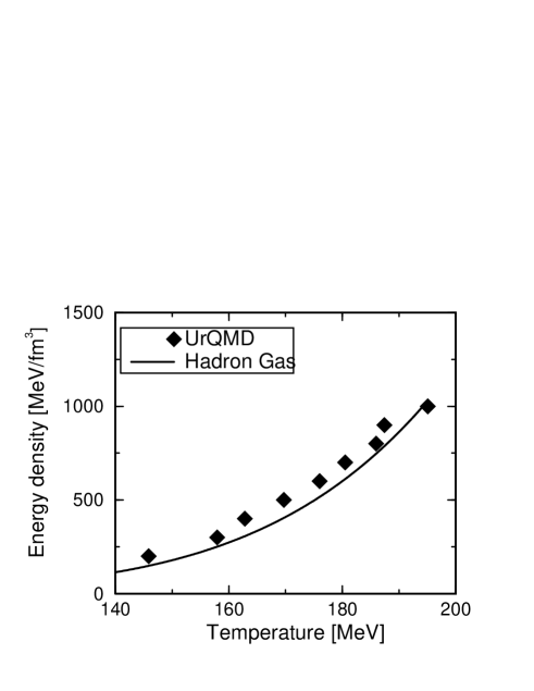
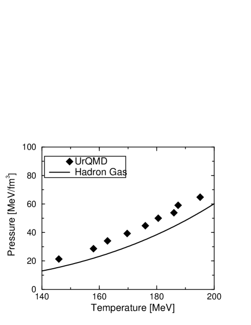
FIG. 5.: The equation of state of a mixed hadron gas at finite temperature ($100$ MeV $<T<200$ MeV) and zero baryon density (0.0 fm^-3). The energy density of mesons is plotted as functions of the temperature. The curve corresponds to the free gas model represented by Eq. (7).

FIG. 6.: The equation of state of a mixed hadron gas at finite temperature ($100$ MeV $<T<200$ MeV) and zero baryon density (0.0 fm^-3). The pressure of pions is plotted as functions of the temperature. The curve corresponds to the free gas model represented by Eq. (8).

Figure 6 shows the energy density versus temperature for mesons. In this figure, the difference between UrQMD results and those for the calculation of the free gas model is negligible. Figure 6 shows the pressure versus temperature for mesons. There is deviation of UrQMD results from the free gas model results especially at high temperatures. The influence of interactions is clear above $T\sim m_{\pi}$. Enhancement of heavy meson resonances grows as the temperature increases.

In a previous study [6]  the limiting value of temperature with increasing energy appeared. As already mentioned this is because of the lack of reversal process of multi–particle production in that study. In this calculation where we try to maintain detailed balanced in UrQMD, this limiting temperature does not appear. This is an important result of taking detailed balance into account.

However, in this simulation the lack of multi–particle production leads to long equilibration times. This is also because we do not have meson–baryon interactions, such as $\pi N\rightarrow R$ and their inverse processes. The enhancement of heavy baryon resonances causes an increase in the abundances of mesons, and vice versa. Heavy resonances readily produce two pions, and thus the enhancement of heavy baryon resonances promotes meson production. Therefore, interactions between mesons and baryons are very important in the study of the properties of a mixed hadron gas. Inclusion of multi–particle interactions would also shorten the equilibration time considerably.

IV Shear Viscosity Coefficient

Transport coefficients such as viscosities, diffusivities and conductivities characterizes the dynamics of fluctuations of dissipative fluxes in a medium. Transport coefficients can be measured, as in the case of condensed matter applications. However in principle they should be calculable theoretically from first principles.

In a weakly coupled theory transport coefficients can be computed in a perturbative expansion, employing either kinetic theory or field theory using Kubo formulas [9, 10, 11, 12, 13, 14, 15]. The resulting Kubo relations [16] express transport coefficients in terms of the zero-frequency slope of spectral densities of current-current, or stress tensor-stress tensor correlation functions,

Monte Carlo simulations for transport coefficients is a powerful tool when studying transport coefficients using Green–Kubo relations. For calculation of transport coefficients of shear viscosity, thermal conductivity, thermal diffusion and mutual diffusion for a binary mixture of hard spheres see [17] and for the calculation of diffusion coefficient of a hadron gas see [8]

Knowledge of various transport coefficients is important in dissipative fluid dynamical models [18]. In this paper we consider the evaluation of shear viscosity coefficient of a hadron gas of mesons and their resonances.

In trying to stay close to the extended irreversible thermodynamic processes we will, however, use the Kubo formulas in fluctuation theory to extract transport coefficients.

In the longitudinal boost–invariant flow the important coefficient is the shear viscosity. In dissipative fluids the expression for the entropy 4–current is governed by transport coefficients and relaxation coefficients. These coefficients determine the strength of the fluctuations of dissipative fluxes about the equilibrium state. The generalized entropy plays an important role in the description of the fluctuations of conserved quantities and of the dissipative fluxes.

Now we calculate the coefficient of shear viscosity. First, the fluctuation–dissipation theorem tells us that shear viscosity $\eta$ is given by the stress tensor correlations [16]

$$\eta={V\over T}\int_{0}^{\infty}\langle\pi_{ij}(t)\cdot\pi_{ij}(t+t^{\prime})\rangle dt^{\prime}\enspace,$$ (9)

where $\pi_{ij}\equiv T_{ij}-\delta_{ij}{\mathcal{P}}$ denotes the traceless part of the stress tensor and ${\mathcal{P}}\equiv{1\over 3}T^{i}_{\;\;i}$ the (local) pressure. The angular brackets stand for equilibrium average, i.e., average over the number of ensemble states and average over the number of particles. The correlation functions are damped exponentially with time (see Fig. 7):

$$\langle\pi_{ij}(t)\cdot\pi_{ij}(t+t^{\prime})\rangle\propto\exp{\left(-\frac{t^{\prime}}{\tau_{\pi}}\right)}.$$ (10)

The solid lines in Fig. 7 are the fits to the correlations and the inverse slope corresponds to the relaxation time. The shear viscosity coefficient can be rewritten in the simple form

$$\eta={V\over T}\langle\pi_{ij}(t)\cdot\pi_{ij}(t)\rangle\tau_{\pi},$$ (11)

where $\tau_{\pi}$ is the relaxation time of the shear flux. In this work we used a box of volume $V=1000$ fm³. The results are insensitive to the box length greater than 6 fm.

To this end, we have to remark that the transport coefficients represents the fluctuations of the dissipative fluxes around an equilibrium state. In terms of fluctuations the Green-Kubo relation (at zero frequency) for shear viscosity can be written as

$$\eta={V\over T}\int_{0}^{\infty}\langle\delta\pi_{ij}(0)\delta\pi_{ij}(t)\rangle dt~{}~{}~{}~{}~{}(i\neq j)\enspace,$$ (12)

In the above equation the fluctuations of shear flux are exponentially damped. They are obtained found from the second differential of the generalized entropy expression [18]

$$\langle\delta\pi_{ij}(0)\delta\pi_{kl}(t)\rangle=\eta T(\tau_{\pi}V)^{-1}\bigtriangleup_{ijkl}\exp(-t/\tau_{\pi})\enspace.$$ (13)

with $\bigtriangleup_{ijkl}=(\delta_{ik}\delta_{jl}+\delta_{il}\delta_{jk}-(2/3)\delta_{ij}\delta_{kl})$. In the limit of vanishing relaxation times, we recover the formulae of Landau and Lifshitz, since in this limit $\tau^{-1}\exp(t/\tau)\rightarrow 2\delta(t)$ with $\delta(t)$ the Dirac delta function. Equation (13) relates the dissipative coefficient $\eta$ to the fluctuations of the fluxes with respect to equilibrium. We see that fluctuations determine the dissipative coefficients. Conversely, transport coefficients determine the strength of the fluctuations.

If the evolution of the fluctuations on the fluxes is described by the Maxwell–Cattaneo (see [18]) relation equations then after integration the above expression for the shear viscosity coefficient reduces to

$$\eta={\tau_{\pi}V\over T}\langle\delta\pi_{ij}(0)\delta\pi_{ij}(0)\rangle\enspace.$$ (14)

In what follows we will use the existing microscopic model, namely UrQMD, to extract the shear viscosity coefficient.

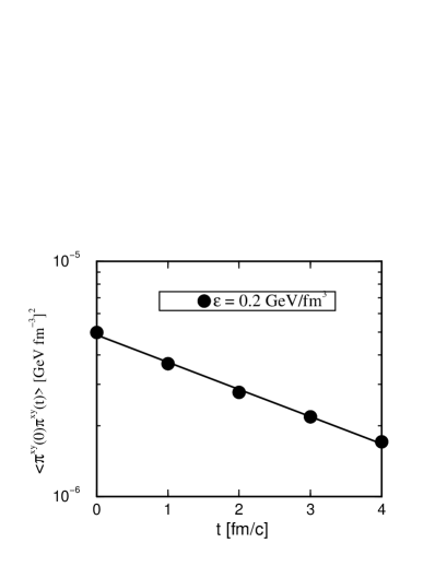
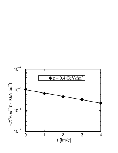
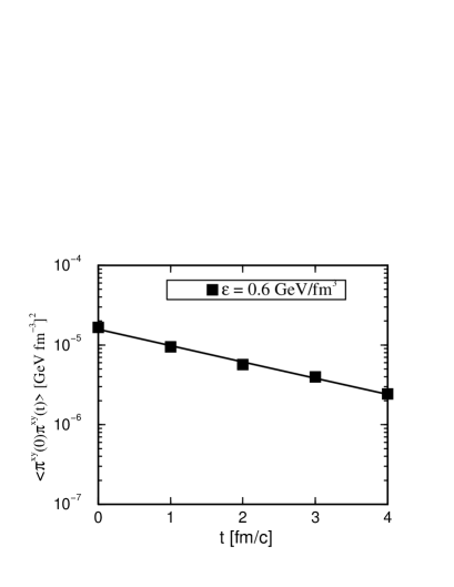
FIG. 7.: Stress–tensor correlation of the mesons as a function of time. The curves are the exponential fits to extract relaxation times

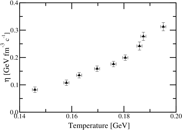
FIG. 8.: Shear viscosity of meson gas as a function of temperature.

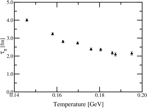
FIG. 9.: The relaxation time for the shear flux of meson gas as a function of temperature.

Figure 8 shows the shear viscosity coefficient results from UrQMD using Kubo relations. As in the variational approach the coefficient grows with temperature. The UrQMD results are about twice those from the variational method. This might be due to the many meson resonances included in UrQMD while in the variational method we only have pions. Also the cross section parameterizations are different in the two approaches. Figure 9 shows the relaxation time for shear flux in a hot pion gas calculated from UrQMD by fitting the shear stress correlations. The dependence of the shear relaxation time on temperature is similar to the one obtained using variational method. The results obtained here are about a factor of two less than variational method results. The reasons are similar to the ones given above for the shear viscosity coefficient.

V Conclusions and outlook

The transport coefficients for a hadron gas can be obtained easily from microscopic transport models such as UrQMD. The study of fluctuations of dissipative fluxes around equilibrium yields Green–Kubo relations which are more easily applied. The use of fluctuations through Kubo relations has the advantage of finding not only the transport coefficients but also the corresponding relaxation times. In addition it is also possible to obtain the relaxation coefficients such as $\beta_{2}$ used in [18].

Since the shear viscosity coefficient for QCD has been calculated by many authors using either kinetic theory or pertubative expansion, it will be interesting to calculate the shear viscosity coefficient for quark gluon plasma using microscopic models in the form of parton cascade models such as VNI/BMS [19]. This is currently under investigation [20].