Causal Theories of Dissipative Relativistic Fluid Dynamics for Nuclear Collisions.

Abstract

Non-equilibrium fluid dynamics derived from the extended irreversible thermodynamics of the causal Müller–Israel–Stewart theory of dissipative processes in relativistic fluids based on Grad’s moment method is applied to the study of the dynamics of hot matter produced in ultra–relativistic heavy ion collisions. The temperature, energy density and entropy evolution are investigated in the framework of the Bjorken boost–invariant scaling limit. The results of these second order theories are compared to those of first order theories due to Eckart and to Landau and Lifshitz and those of zeroth order (perfect fluid) due to Euler. In the presence of dissipation perfect fluid dynamics is no longer valid in describing the evolution of the matter. First order theories fail in the early stages of evolution. Second order theories give a better description in good agreement with transport models. It is shown in which region the Navier–Stokes–Fourier laws (first order theories) are a reasonable limiting case of the more general extended thermodynamics (second order theories).

I Introduction

The study of space–time evolution and non–equilibrium properties of matter produced in high energy heavy ion collisions, such as those at the Relativistic Heavy Ion Collider (RHIC) at Brookhaven National Laboratory, USA and the Large Hadron Collider (LHC) at CERN, Geneva using relativistic dissipative fluid dynamics are of importance in understanding the observables.

High energy heavy ion collisions offer the opportunity to study the properties of hot and dense matter. To do so we must follow its space–time evolution, which is affected not only by the equation of state but also by dissipative, non–equilibrium processes. Thus we need to know the transport coefficients such as viscosities, conductivities, and diffusivities. We also need to know the relaxation times for various dissipative processes under consideration. Knowledge of the various time and length scales is of central importance to help us decide whether to apply fluid dynamics (macroscopic) or kinetic theory (microscopic) or a combination of the two. The use of fluid dynamics as one of the approaches in modelling the dynamic evolution of nuclear collisions has been successful in describing many of the observables [3, 4]. The assumptions and approximations of the fluid dynamical models are another source for uncertainties in predicting the observables. So far most work has focused on the ideal or perfect fluid and/or multi-fluid dynamics. In this work we apply the relativistic dissipative fluid dynamical approach. It is known even from non–relativistic studies [5] that dissipation might affect the observables.

The first theories of relativistic dissipative fluid dynamics are due to Eckart [6] and to Landau and Lifshitz [7]. The difference in formal appearance stems from different choices for the definition of the hydrodynamical 4–velocity. These conventional theories of dissipative fluid dynamics are based on the assumption that the entropy four–current contains terms up to linear order in dissipative quantities and hence they are referred to as first order theories of dissipative fluids. The resulting equations for the dissipative fluxes are linearly related to the thermodynamic forces, and the resulting equations of motion are parabolic in structure, from which we get the Fourier–Navier–Stokes equations. They have the undesirable feature that causality may not be satisfied. That is, they may propagate viscous and thermal signals with speeds exceeding that of light.

Extended theories of dissipative fluids due to Grad [8], Müller [9], and Israel and Stewart [10] were introduced to remedy some of these undesirable features. These causal theories are based on the assumption that the entropy four–current should include terms quadratic in the dissipative fluxes and hence they are referred to as second order theories of dissipative fluids. The resulting equations for the dissipative fluxes are hyperbolic and they lead to causal propagation of signals [10, 11]. In second order theories the space of thermodynamic quantities is expanded to include the dissipative quantities for the particular system under consideration. These dissipative quantities are treated as thermodynamic variables in their own right.

A qualitative study of relativistic dissipative fluids for applications to relativistic heavy ions collisions has been done using these first order theories [12, 13, 14, 15, 16, 17]. The application of second order theories to nuclear collisions has just begun [18, 19, 20], and the results of relativistic fluid dynamics can also be compared to the prediction of spontaneous symmetry breaking results [21].

The rest of the article is outlined as follows. In section II we review the basics of equilibrium thermodynamics and perfects fluids. In III the basic formulation of relativistic dissipative fluid dynamics will briefly introduced. In section IV we introduce the special hydrodynamical model of Bjorken. In section V we discuss the results of perfect fluids. In section VI we discuss the results of dissipative fluids. We first discuss the results of first order theories and then for the second order theories. In section VII we summarize the results and discuss the need for hyperbolic theories for relativistic dissipative fluids.

Throughout this article we adopt the units $\hbar=c=k_{\rm B}=1$. The sign convention used follows the time-like convention with the signature $(+,-,-,-)$, and if $u^{\alpha}$ is a time-like vector, $u^{\alpha}u_{\alpha}>0$. The metric tensor is always taken to be $g^{\mu\nu}=\mbox{diag}(+1,-1,-1,-1)$, the Minkowski tensor. Upper greek indices are contravariant, lower greek indices covariant. The greek indices used in 4–vectors go from 0 to 3 ($t,x,y,z$) and the roman indices used in 3–vectors go from 1 to 3 ($x,y,z$). The scalar product of two 4-vectors $a^{\mu}\,,\,\,b^{\mu}$ is denoted by $a^{\mu}\,g_{\mu\nu}\,b^{\nu}\equiv a^{\mu}\,b_{\mu}\equiv a\cdot b$. The scalar product of two 3-vectors is denoted by bold type, namely, $\mbox{\boldmath${a}$},\,\mbox{\boldmath${b}$}$, $\mbox{\boldmath${a}$}\cdot\mbox{\boldmath${b}$}$. The notations $A^{(\alpha\beta)}\equiv(A^{\alpha\beta}+A^{\beta\alpha})/2$ and $A^{[\alpha\beta]}\equiv(A^{\alpha\beta}-A^{\beta\alpha})/2$ denote symmetrization and antisymmetrization respectively. The 4–derivative is denoted by ${\partial}_{\alpha}\equiv{\partial}/{\partial}x^{\alpha}$. Contravariant components of a tensor are found from covariant components by $g_{\alpha\beta}A^{\alpha}=A_{\beta}$, $g_{\mu\alpha}g_{\nu\beta}F^{\alpha\beta}=F_{\mu\nu}$ and so on.

II Basics of Equilibrium Relativistic Fluid Dynamics

The basic ingredients of equilibrium thermodynamics are the energy density $\varepsilon$, the number density $n$, and the entropy density $s$. The pressure $p$ can be related to the other state variables. In this work these basic ingredients will be referred to as the primary thermodynamic variables. From the equation of state $s=s(\varepsilon,n)$, the temperature $T$ and chemical potential $\mu$ emerge as partial derivatives:

$$\varepsilon+p = Ts+\mu n\enspace,$$ (1)

$$T{\rm d}s = {\rm d}\varepsilon-\mu{\rm d}n\enspace.$$ (2)

The chemical potential $\mu$ is the energy required to inject one extra particle reversibly into a fixed volume. The fundamental relation (1) then yields the last unknown thermodynamic function $p$. Next we introduce the thermal potential $\alpha$ and inverse-temperature $\beta$ by the definitions

$$\alpha\equiv{\mu\over T}\,\,\,\,,\,\,\,\,\beta\equiv{1\over T}\enspace.$$ (3)

Then equations (1) and (2) take the form

$$s = \beta(\varepsilon+p)-\alpha n\enspace,$$ (4)

$${\rm d}s = \beta{\rm d}\varepsilon-\alpha{\rm d}n\enspace.$$ (5)

In relativistic fluid dynamics it is advantageous to cast the thermodynamic quantities in terms of covariant objects, namely, the energy–momentum tensor $T^{\mu\nu}$, the 4–vector number current $N^{\mu}$ representing the net charge current, and the entropy 4–current $S^{\mu}$. For heavy ion collisions, the conserved charge is usually taken to be the net baryon number. The covariant quantities are expressible in terms of a unique hydrodynamical 4–velocity $u^{\mu}$ (normalized as $u_{\mu}u^{\mu}=1$) and the primary state variables ($\varepsilon\,,\,\,n\,,\,\,p\,,\,\,s$).

$$N^{\mu} = nu^{\mu}\enspace,$$ (6)

$$T^{\mu\nu} = \varepsilon u^{\mu}u^{\nu}-p\bigtriangleup^{\mu\nu}\enspace,$$ (7)

$$S^{\mu} = su^{\mu}\enspace.$$ (8)

Here $\bigtriangleup^{\mu\nu}\equiv g^{\mu\nu}-u^{\mu}u^{\nu}$ is the spatial projection tensor orthogonal to $u^{\mu}$, $u^{\mu}=\gamma(1,{\bf v})$ ($\gamma=1/\sqrt{1-{\bf v}^{2}}$) is the (local) 4-velocity of the fluid, and $g^{\mu\nu}$ the Minkowski metric. The pressure can be related to the energy density and the number density by an equation of state. The equilibrium state will therefore be described by 5 parameters $(\varepsilon\,,\,\,n\,,\,\,u^{\mu})$.

The thermodynamical relations can be written in a form that involves the covariant objects $S^{\mu},N^{\mu}$ and $T^{\mu\nu}$ directly as basic variables:

$${\rm d}S^{\mu}=-\alpha{\rm d}N^{\mu}+\beta_{\nu}{\rm d}T^{\mu\nu}\enspace,$$ (9)

where

$$\beta_{\nu}\equiv\beta u_{\nu}={u_{\nu}\over T}\enspace,$$ (10)

defines the inverse–temperature 4–vector. From (1) we have immediately

$$S^{\mu}=p\beta^{\mu}-\alpha N^{\mu}+\beta_{\nu}T^{\mu\nu}\enspace.$$ (11)

It follows from (9) and (11) that

$${\rm d}(p\beta^{\mu})=N^{\mu}{\rm d}\alpha-T^{\mu\nu}{\rm d}\beta_{\nu}\enspace.$$ (12)

Thus the basic variables $N^{\mu},\,\,T^{\mu\nu}$ and $S^{\mu}$ can all be generated from partial derivatives of the fugacity 4–vector $p(\alpha,\beta)\beta^{\mu}$, once the equation of state is known.

In the covariant formulation the hydrodynamical velocity is co–opted in a natural way as an extra thermodynamical variable. The covariant equations, expressed directly in terms of the basic conserved variables $N^{\mu}$ and $T^{\mu\nu}$, can be manipulated more easily and transparently. Formulations for deviation from equilibrium can be carried out without much difficulty by making an assumption or requirement that (11) remains valid at least to first order in deviations (see the next section).

The four–divergence of the energy–momentum tensor, the number 4–current, and the entropy 4–current vanish. That is, the energy and momentum, the number density, and the entropy density are all conserved. The covariant forms of particle, energy, momentum and entropy conservation are

$${\partial}_{\alpha}N^{\alpha}=0 \quad\Rightarrow\quad u^{\alpha}{\partial}_{\alpha}n+n{\partial}_{\alpha}u^{\alpha}=0\quad\enspace,$$ (13)

$$u_{\alpha}{\partial}_{\beta}T^{\alpha\beta}=0 \quad\Rightarrow\quad u^{\alpha}{\partial}_{\alpha}\varepsilon+(\varepsilon+p){\partial}_{\alpha}u^{\alpha}=0\enspace,$$ (14)

$$\bigtriangledown^{\alpha}_{\beta}{\partial}_{\lambda}T^{\beta\lambda}=0 \quad\Rightarrow\quad (\varepsilon+p)u^{\beta}{\partial}_{\beta}u^{\alpha}-\bigtriangleup^{\alpha\beta}{\partial}_{\beta}p=0\enspace,$$ (15)

$${\partial}_{\alpha}S^{\alpha}=0 \quad\Rightarrow\quad u^{\alpha}{\partial}_{\alpha}s+s{\partial}_{\alpha}u^{\alpha}=0\enspace.$$ (16)

Eq. (16) means that the entropy is conserved in ideal fluid dynamics. Note that $s$ is constant along fluid world-lines, and not throughout the fluid in general. If $s$ is the same constant on each world-line, that is, if $\bigtriangledown_{\alpha}s=0$ as well as $\dot{s}=0$, so that ${\partial}_{\alpha}s=0$, then the fluid is called isentropic. Thus perfect fluids in equilibrium generate no entropy and no frictional type heating because their dynamics is reversible and without dissipation. For many processes in nuclear collisions a perfect fluid model is adequate. However, real fluids behave irreversibly, and some processes in heavy ion reactions may not be understood except as dissipative processes, requiring a relativistic theory of dissipative fluids. An equilibrium state is characterized by the absence of viscous stresses, heat flow and diffusion and maximum entropy principle, while a non–equilibrium state is characterized by the principle of nondecreasing entropy which arises due to the presence of dissipative fluxes.

Perfect fluid dynamics has been successful in describing most of the observables [3, 4, 22]. The current status of ideal hydrodynamics in describing observables can be found in the latest Quark Matter Proceedings [1] and in [23, 24]. Already at the level of ideal fluid approximation constructing numerical solution scheme to the equations is not an easy task. This is due to the nonlinearity of the system of conservation equations. Much work has been done in ideal hydrodynamics for heavy ion collision simulations (see e.g., [25]).

III Non-equilibrium/dissipative Relativistic Fluid Dynamics

We give a covariant formulation of non–equilibrium thermodynamics. The central role of entropy is highlighted. Non–equilibrium effects are introduced by enlarging the space of basic independent variables through the introduction of non–equilibrium variables, such as dissipative fluxes appearing in the conservation equations. The next step is to find evolution equations for these extra variables. Whereas the evolution equations for the equilibrium variables are given by the usual conservation laws, no general criteria exist concerning the evolution equations of the dissipative fluxes, with the exception of the restriction imposed on them by the second law of thermodynamics.

A natural way to obtain the evolution equations for the fluxes from a macroscopic basis is to generalize the equilibrium thermodynamic theories. That is, we assume the existence of a generalized entropy which depends on the dissipative fluxes and on the equilibrium variables as well. Restrictions on the form of the evolution equations are then imposed by the laws of thermodynamics. From the expression for generalized entropy one then can derive the generalized equations of state, which are of interest in the description of system under consideration. The phenomenological formulation of the transport equations for the first order and second order theories is accomplished by combining the conservation of energy–momentum and particle number with the Gibbs equation. One then obtains an expression for the entropy 4–current, and its divergence leads to entropy production. Because of the enlargement of the space of variables the expressions for the energy-momentum tensor $T^{\mu\nu}$, particle 4–current $N^{\mu}$, entropy 4-current $S^{\mu}$, and the Gibbs equation contain extra terms. Transport equations for dissipative fluxes are obtained by imposing the second law of thermodynamics, that is, the principle of nondecreasing entropy. The kinetic approach is based on Grad’s 14–moment method [8]. For a review on generalization of the 14–moment method to a mixture of several particle species see [26]. For applications and discussions of the moment method in kinetic and transport theory of gases see e.g. [27] and for applications in astrophysics and cosmology see e.g. [28].

In the early stages of relativistic nuclear collisions we want to be able to describe phenomena at frequencies comparable to the inverse of the relaxation times of the fluxes. At such time scales, these fluxes must be included in the set of basic independent variables. In order to model dissipative processes we need non–equilibrium fluid dynamics or irreversible thermodynamics. A satisfactory approach to irreversible thermodynamics is via non–equilibrium kinetic theory. In this work we will, however, follow a phenomenological approach. Whenever necessary we will point out how kinetic theory supports many of the results and their generalization. A complete discussion of irreversible thermodynamics is given in the monographs [29, 30, 31], where most of the theory and applications are non–relativistic but includes relativistic thermodynamics. A relativistic, but more advanced, treatment may be found in [32, 33, 34]. In this work we will present a simple introduction to these features, leading up to a formulation of relativistic causal fluid dynamics that can be used for applications in nuclear collisions.

A Basic Features of Irreversible Thermodynamics and Imperfect Fluids

The basic formulation of relativistic hydrodynamics can be found in the literature (see for example [7, 35, 36, 37]). We consider a simple fluid and no electromagnetic fields. This fluid is characterized by,

$$N_{A}^{\mu}(x) \makebox[21.68121pt][l]{}\mbox{particle 4--current}\enspace,$$ (17)

$$T^{\mu\nu}(x) \makebox[21.68121pt][l]{}\mbox{energy--momentum tensor}\enspace,$$ (18)

$$S^{\mu}(x) \makebox[21.68121pt][l]{}\mbox{entropy 4--current}\enspace,$$ (19)

where $A=1,...,r$ for the $r$ conserved net charge currents, such as electric charge, baryon number, and strangeness. $N_{A}^{\mu}$ and $T^{\mu\nu}$ represent conserved quantities:

$$\partial_{\mu}N_{A}^{\mu} = 0\enspace,$$ (20)

$$\partial_{\mu}T^{\mu\nu} = 0\enspace.$$ (21)

The above equations are the local conservation of net charge and energy–momentum. They are the equations of motion of a relativistic fluid. There are $4+r$ equations and $10+4r$ independent unknown functions. The second law of thermodynamics requires

$$\partial_{\mu}S^{\mu}\geq 0\enspace,$$ (22)

and it forms the basis for the development of the extended irreversible thermodynamics.

We now perform a tensor decomposition of $N^{\mu},\,T^{\mu\nu},$ and $S^{\mu}$ with respect to an arbitrary, time–like, 4–vector $u^{\mu}$, normalized as $u^{\mu}u_{\mu}=1$, and the projection onto the 3-space $\bigtriangleup^{\mu\nu}$ orthogonal to $u^{\mu}$. Note that

$$\bigtriangleup^{\mu\nu}=\bigtriangleup^{\nu\mu}\,,\,\,\bigtriangleup^{\mu\nu}u_{\nu}=0\,,\,\,\bigtriangleup^{\mu\alpha}\bigtriangleup_{\alpha}^{\nu}=\bigtriangleup^{\mu\nu}\,,\,\,\,\bigtriangleup^{\nu}_{\nu}=3\enspace.$$ (23)

The tensor decomposition reads:

$$N^{\mu} = n\,u^{\mu}+V^{\mu}\enspace,$$ (24)

$$T^{\mu\nu} = \varepsilon\,u^{\mu}u^{\nu}-p\bigtriangleup^{\mu\nu}+2\,W^{(\mu}\,u^{\nu)}+t^{\mu\nu}\enspace,$$ (25)

$$S^{\mu} = su^{\mu}+\Phi^{\mu}\enspace,$$ (26)

where we have defined

$$W^{\mu} = q^{\mu}+h\,V^{\mu}\enspace,$$ (27)

$$t^{\mu\nu} = \pi^{\mu\nu}-\Pi\,\bigtriangleup^{\mu\nu}\enspace.$$ (28)

Here $h$ is the enthalpy per particle defined by

$$h=\frac{(\varepsilon+p)}{n}\enspace.$$ (29)

The dissipative fluxes satisfy the following orthogonality relations:

$$u_{\mu}V^{\mu}=0\,,\,\,u_{\mu}q^{\mu}=0\,,\,\,u_{\mu}\,W^{\mu}=0\,,\,\,u_{\mu}\,t^{\mu\nu}=0\,,\,\,\pi^{\nu}_{\nu}=0\enspace.$$ (30)

In the local rest frame (LRF) defined by $u^{\mu}=(1,\bf{0})$ the quantities appearing in the decomposed tensors have the following meanings:

$$n \equiv \makebox[72.26999pt][l]{$u_{\mu}N^{\mu}$}\mbox{net density of charge}\enspace,$$ (31)

$$V^{\mu} \equiv \makebox[72.26999pt][l]{$\bigtriangleup^{\mu}_{\nu}N^{\nu}$}\mbox{net flow of charge}\enspace,$$ (32)

$$\varepsilon \equiv \makebox[72.26999pt][l]{$u_{\mu}T^{\mu\nu}u_{\nu}$}\mbox{energy density}\enspace,$$ (33)

$$p+\Pi \equiv \makebox[72.26999pt][l]{$\displaystyle-\frac{1}{3}\bigtriangleup_{\mu\nu}T^{\mu\nu}$ }\mbox{pressure}\enspace,$$ (34)

$$W^{\mu} \equiv \makebox[72.26999pt][l]{$u_{\nu}T^{\nu\lambda}\bigtriangleup^{\mu}_{\lambda}$}\mbox{energy flow}\enspace,$$ (35)

$$q^{\mu} \equiv \makebox[72.26999pt][l]{$W^{\mu}-hV^{\mu}$}\mbox{heat flow}\enspace,$$ (36)

$$\pi^{\mu\nu} \equiv \makebox[72.26999pt][l]{$T^{\langle\mu\nu\rangle}$ }\mbox{stress tensor}\enspace,$$ (37)

$$s \equiv \makebox[72.26999pt][l]{$u_{\mu}\,S^{\mu}$}\mbox{entropy density}\enspace,$$ (38)

$$\Phi^{\mu} \equiv \makebox[72.26999pt][l]{$\bigtriangleup^{\mu}_{\nu}S^{\nu}$}\mbox{entropy flux}\enspace.$$ (39)

The angular bracket notation, representing the symmetrized spatial and traceless part of the tensor, is defined by

$$A^{\langle\mu\nu\rangle}\equiv\left[\frac{1}{2}\left(\bigtriangleup^{\mu}_{\sigma}\bigtriangleup^{\nu}_{\tau}+\bigtriangleup^{\mu}_{\tau}\bigtriangleup^{\nu}_{\sigma}\right)-\frac{1}{3}\bigtriangleup^{\mu\nu}\bigtriangleup_{\sigma\tau}\right]A^{\sigma\tau}\enspace.$$ (40)

The space–time derivative decomposes into

$$\partial^{\mu}=u^{\mu}\mbox{D}+\bigtriangledown^{\mu}\,,~{}~{}~{}~{}~{}u^{\mu}\bigtriangledown_{\mu}=0\enspace,$$ (41)

where

$$D \equiv \makebox[72.26999pt][l]{$u^{\mu}\partial_{\mu}$}\mbox{convective time derivative}\enspace,$$ (42)

$$\bigtriangledown^{\mu} \equiv \makebox[72.26999pt][l]{$\bigtriangleup^{\mu\nu}\partial_{\nu}$}\mbox{gradient operator}\enspace.$$ (43)

In the LRF the two operators attain the given meanings. In this rest frame the projector becomes

$$\bigtriangleup_{\mu\nu}=\bigtriangleup^{\mu\nu}=\mbox{diag}(0,-1,-1,-1),~{}~{}~{}~{}~{}~{}~{}~{}~{}~{}\bigtriangleup^{\mu}_{\nu}=\mbox{diag}(0,1,1,1)\enspace.$$ (44)

In the LRF the heat flow has spatial components only and the pressure tensor defined by $P^{\mu\nu}\equiv\bigtriangleup^{\mu}_{\sigma}T^{\sigma\tau}\bigtriangleup^{\nu}_{\tau}=-(p\bigtriangleup^{\mu\nu}+\Pi)+\pi^{\mu\nu}$ is also purely spatial.

So far, $u^{\mu}$ is arbitrary. It has the following properties. Differentiating $u_{\mu}u^{\mu}=1$ with respect to space–time co-ordinates, ${\partial}_{\mu}\equiv({\partial}/{\partial}x^{\mu})\equiv({\partial}_{t},\mbox{\boldmath${\nabla}$})$, yields

$$u_{\mu}{\partial}_{\nu}u^{\mu}=0\enspace,$$ (45)

which is a useful relation.

There are two choices for $u^{\mu}$ [32]. It can be taken parallel to the particle flux $N^{\mu}$,

$$u^{\mu} \equiv \frac{N^{\mu}}{\sqrt{N^{\mu}N_{\mu}}}\enspace,$$ (46)

$$N^{\mu} = nu^{\mu}\enspace.$$ (47)

This is known as the Eckart or particle frame and in this frame $V^{\mu}=0$. It can also be taken to be parallel to the energy flow,

$$u^{\mu} \equiv \frac{T^{\mu}_{\nu}u^{\nu}}{\sqrt{u^{\alpha}T_{\alpha}^{\beta}T_{\beta\gamma}u^{\gamma}}}\enspace,$$ (48)

$$u_{\nu}T^{\mu\nu} = \varepsilon u^{\mu}\enspace.$$ (49)

This is known as the Landau and Lifshitz or energy frame and in this frame $W^{\mu}=0$. This implies that $q^{\mu}=-hV^{\mu}$.

The two choices of velocity 4–flow have different computational advantage of each of the formulations. The Landau–Lifshitz formalism is convenient to employ since it reduces the energy–momentum tensor to a simpler form. The price for this is the implicit definition of the 4–velocity. The Eckart formalism has the advantage when one wants to have simple integration of particle conservation law. This choice is also more intuitive than that of Landau–Lifshitz. For a system with no net charge, the 4–velocity in the Eckart formalism is not well–defined and therefore in general under this situation one should use the Landau–Lifshitz formalism. The Landau–Lifshitz formalism is also advantageous in the case of mixtures.

Let us consider the Eckart definition of 4-velocity. With respect to this frame the particle number 4-current and energy–momentum tensor thus decomposes as follows:

$$N^{\mu} = nu^{\mu}\enspace,$$ (50)

$$T^{\mu\nu} = \varepsilon u^{\mu}u^{\nu}+2q^{(\mu}u^{\nu)}+P^{\mu\nu}\enspace,$$ (51)

$$P^{\mu\nu} = P^{\nu\mu}~{}~{}~{},~{}~{}~{}P^{\mu\nu}u_{\mu}=q^{\mu}u_{\mu}=0\enspace,$$ (52)

$$P^{\mu\nu} = -(p+\Pi)\bigtriangleup^{\mu\nu}+\pi^{\mu\nu}~{}~{}~{},~{}~{}~{}\bigtriangleup^{\mu\nu}\pi_{\mu\nu}=0\enspace.$$ (53)

Successive terms on the right hand side of (53) represent the thermodynamical pressure, bulk stress and shear stress measured by an observer in the Eckart frame.

B Conservation Laws

We will now consider one type of charge, namely, the net baryon number. We also consider the Eckart frame for the 4-velocity definition. We insert the expressions for the number 4–current and the energy–momentum tensor in the conservation laws and project them onto the four velocity and the projection tensor. Using the orthogonality properties given in the previous section we obtain the following conservation laws. The equation of continuity (net charge conservation) $\partial_{\mu}N^{\mu}\equiv 0$, equation of motion (momentum conservation) $\bigtriangleup^{\mu}_{\nu}\partial_{\lambda}T^{\nu\lambda}\equiv 0$, and the equation of energy (energy conservation) $u_{\mu}\partial_{\nu}T^{\mu\nu}\equiv 0$ are, respectively,

$$\mbox{D}\,n = -n\,\bigtriangledown_{\mu}\,u^{\mu}\enspace,$$ (54)

$$(\varepsilon+p+\Pi)\mbox{D}\,u^{\mu} = \bigtriangledown^{\mu}(p+\Pi)-\bigtriangleup^{\mu}_{\nu}\bigtriangledown_{\sigma}\pi^{\nu\sigma}+\pi^{\mu\nu}\mbox{D}\,u_{\nu}$$ (56)

$$-[\bigtriangleup^{\mu}_{\nu}\mbox{D}\,q^{\nu}+2q^{(\mu}\bigtriangledown_{\nu}u^{\nu)}]\enspace,$$

$$\mbox{D}\,\varepsilon = -(\varepsilon+p+\Pi)\bigtriangledown_{\mu}u^{\mu}+\pi^{\mu\nu}\bigtriangledown_{\langle\nu}u_{\mu\rangle}$$ (58)

$$-\bigtriangledown_{\mu}q^{\mu}+2q^{\mu}\mbox{D}u_{\mu}\enspace.$$

There are 14 unknowns, $n,\,\varepsilon,\Pi,q^{\mu},\pi^{\mu\nu}$, and $u^{\mu}$ and 5 equations. To close the system of equations we need to obtain 9 additional equations (for dissipative fluxes) in addition to the 5 conservation equations (for primary variables) we already know. The derivation of the 9 equations will be presented in the following sections.

C Entropy 4-current and the generalized Gibbs equation

From the phenomenological treatment of deriving the 9 additional equations we need the expression for the out–of–equilibrium entropy 4-current. The off-equilibrium entropy 4-current $S^{\mu}(N^{\mu},T^{\mu\nu})$ takes the form [10]

$$S^{\mu}=p(\alpha,\beta)\beta^{\mu}-\alpha N^{\mu}+\beta_{\nu}T^{\mu\nu}+Q^{\mu}(\delta N^{\mu},\,\,\delta T^{\mu\nu},\,\,...)$$ (59)

where $Q^{\mu}$ is a function of deviations $\delta N^{\mu}$ and $\delta T^{\mu\nu}$ from local equilibrium

$$\delta T^{\mu\nu}=T^{\mu\nu}-T^{\mu\nu}_{eq}\,\,\,\,,\,\,\,\,\delta N^{\mu}=N^{\mu}-N_{eq}^{\mu}\enspace,$$ (60)

containing all the information about viscous stresses and heat flux in the off–equilibrium state.

Since the equilibrium pressure is only known as a function of the equilibrium energy density and equilibrium net charge density we need to match/fix the equilibrium pressure to the actual state. We do this by requiring that the equilibrium energy density and the equilibrium net charge density be equal to the off–equilibrium energy density and off–equilibrium net charge density. In Eckart’s formalism this is equivalent to

$$\delta T^{\mu\nu}u_{\mu}u_{\nu}=\delta N^{\mu}u_{\mu}.$$ (61)

With the help of the expression for the divergence of $p\beta^{\mu}$

$${\partial}_{\mu}(p\beta^{\mu})=N^{\mu}_{eq}{\partial}_{\mu}\alpha-T^{\mu\nu}_{eq}{\partial}_{\mu}\beta_{\nu}\enspace,$$ (62)

and the conservation laws for $N^{\mu}$ and for $T^{\mu\nu}$ the generalized second law of thermodynamics becomes

$${\partial}_{\mu}S^{\mu}=-(\delta N^{\mu}){\partial}_{\mu}\alpha+\delta T^{\mu\nu}{\partial}_{\mu}\beta_{\nu}+{\partial}_{\mu}Q^{\mu}\enspace.$$ (63)

Once a detailed form of $Q^{\mu}$ is specified, linear relations between irreversible fluxes ($\delta N^{\mu}$, $\delta T^{\mu\nu}$) and gradients (${\partial}_{(\mu}\beta_{\nu)}$, ${\partial}_{\mu}\alpha$) follow by imposing the second law of thermodynamics, namely, that the entropy production be positive. The key to a complete phenomenological theory thus lies in the specification of $Q^{\mu}$.

D Standard Relativistic Dissipative Fluid Dynamics

The standard Landau–Lifshitz and Eckart theories make the simplest possible assumption about $Q^{\mu}$. That it is linear in the dissipative quantities $(\Pi,\,q^{\mu},\pi^{\mu\nu})$. In kinetic theory this amounts to Taylor expanding the entropy 4–current expression up to first order in deviations from equilibrium. This leads to an expression of entropy 4–current which is just a linear function of the heat flux.

This can be understood as follows: Take a simple fluid with particle current $N^{\mu}$. Let us choose $\beta^{\mu}=u^{\mu}/T$ parallel to the current $N^{\mu}$ of the given off–equilibrium state, so we are in the Eckart frame. Projecting (59) onto the 3-space orthogonal to $u^{\mu}$ gives

$$\Phi^{\mu}\equiv\bigtriangleup^{\mu}_{\nu}S^{\nu}=\beta q^{\mu}+Q^{\nu}\bigtriangleup^{\mu}_{\nu}~{}~{}~{},~{}~{}~{}~{}~{}q^{\mu}=u_{\nu}T^{\nu\lambda}\bigtriangleup^{\mu}_{\lambda}\enspace,$$ (64)

so that

$$\Phi^{\mu}=q^{\mu}/T+\mbox{second order terms}\enspace,$$ (65)

which, to linear order, is just the standard relation between entropy flux $\Phi^{\mu}$ and heat flux $q^{\mu}$. From (64) this implies that the entropy flux $\Phi^{\mu}$ is a strictly linear function of heat flux $q^{\mu}$, and depends on no other variables; also that the off–equilibrium entropy density depends only on the densities $\varepsilon$ and $n$ and is given precisely by the equation of state $s=s_{eq}(\varepsilon,n)$.

Alternatively we may begin with the ansatz for the entropy 4–current $S^{\mu}$: In the limit of vanishing $\Pi,\,q^{\mu},$ and $\pi^{\mu\nu}$ the entropy 4–current must reduce to the one of ideal fluid. The only non–vanishing 4–vector which can be formed from the available tensors $u^{\mu},\,q^{\mu}$ and $\pi^{\mu\nu}$ is $\beta q^{\mu}$ where $\beta$ is arbitrary but it turns out to be nothing else but the inverse temperature. Thus the first order expression for the entropy 4–current in the Eckart frame is given by

$$S^{\mu}=su^{\mu}+{q^{\mu}\over T}\enspace,$$ (66)

and one immediately realizes that

$$\Phi^{\mu}={q^{\mu}\over T}\enspace,$$ (67)

is the entropy flux. Using the expressions for $N^{\mu}$, $T^{\mu\nu}$ and $S^{\mu}$ in the second law of thermodynamics ${\partial}_{\mu}S^{\mu}\geq 0$ and using the conservation laws $u_{\nu}\partial_{\mu}T^{\mu\nu}=0$, $\partial_{\mu}N^{\mu}=0$ and the Gibbs equation

$${\partial}_{\mu}(p\beta^{\mu})=N^{\mu}{\partial}_{\mu}\alpha-T^{\mu\nu}{\partial}_{\mu}\beta_{\nu}\enspace,$$ (68)

the divergence of (66) gives the following expression for entropy production

$$T\,\partial_{\mu}S^{\mu}=q^{\mu}(\bigtriangledown_{\mu}\beta+D\,u_{\mu})+\pi^{\mu\nu}\bigtriangledown_{\mu}u_{\nu}+\Pi\bigtriangledown_{\mu}u^{\mu}\geq 0\enspace.$$ (69)

Notice that the equilibrium conditions (i.e., the bulk free and shear free of the flow and the constancy of the thermal potential,i.e., no heat flow) lead to the vanishing of each factor multiplying the dissipative terms on the right, and therefore lead to ${\partial}_{\alpha}S^{\alpha}=0$. The expression (69) splits into three independent, irreducible pieces:

$$\Pi X-q^{\mu}X_{\mu}+\pi^{\mu\nu}X_{\langle\mu\nu\rangle}\geq 0\enspace,$$ (70)

where

$$X = -\bigtriangledown_{\mu}u^{\mu}\enspace,$$ (71)

$$X^{\mu} = {\bigtriangledown^{\mu}T\over T}-Du^{\mu}\enspace,$$ (72)

$$X^{\langle\mu\nu\rangle} = \left[{1\over 2}\left(\bigtriangleup^{\mu}_{\sigma}\bigtriangleup^{\nu}_{\tau}+\bigtriangleup^{\nu}_{\sigma}\bigtriangleup^{\mu}_{\tau}\right)-{1\over 3}\bigtriangleup^{\mu\nu}\bigtriangleup_{\sigma\tau}\right]\bigtriangledown^{\sigma}u^{\tau}\enspace.$$ (73)

The angular brackets extract the purely spatial, trace-free part of the tensor. From the second law of thermodynamics, ${\partial}_{\mu}S^{\mu}\geq 0$, we see that the simplest way to satisfy the bilinear expression (69) is to impose the following linear relationships between the thermodynamic fluxes $\Pi,q^{\mu},\pi^{\mu\nu}$ and the corresponding thermodynamic forces $\bigtriangledown_{\mu}u^{\mu},\bigtriangledown^{\mu}\ln T-Du^{\mu},\bigtriangledown^{\langle\mu}u^{\nu\rangle}$:

$$\Pi \equiv -\zeta\bigtriangledown_{\mu}u^{\mu}\enspace,$$ (74)

$$q^{\mu} \equiv \lambda T\left(\frac{\bigtriangledown^{\mu}T}{T}-Du^{\mu}\right)=-{\lambda\,n\,T^{2}\over\varepsilon+p}\bigtriangledown^{\mu}\left(\frac{\mu}{T}\right)\enspace,$$ (75)

$$\pi^{\mu\nu} \equiv 2\eta\bigtriangledown^{\langle\mu}u^{\nu\rangle}\enspace.$$ (76)

That is, we assume that the dissipative fluxes are linear and purely local functions of the gradients. We then obtain uniquely, if the equilibrium state is isotropic (Curie’s principle), the above linear expressions.

These are the constitutive equations for dissipative fluxes in the standard Eckart theory of relativistic irreversible thermodynamics. They are relativistic generalizations of the corresponding Newtonian laws. The linear laws allow us to identify the thermodynamic coefficients, namely the bulk viscosity $\zeta(\varepsilon,n)$, the thermal conductivity $\lambda(\varepsilon,n)$ and the shear viscosity $\eta(\varepsilon,n)$.

Given the linear constitutive equations (74) – (76), the entropy production rate (69) becomes

$${\partial}_{\mu}S^{\mu}={\Pi^{2}\over\zeta T}-{q_{\mu}q^{\mu}\over\lambda T^{2}}+{\pi_{\mu\nu}\pi^{\mu\nu}\over 2\eta T}\geq 0$$ (77)

which is guaranteed to be non–negative provided that

$$\zeta\geq 0\,,\quad\lambda\geq 0\,,\quad\eta\geq 0\enspace.$$ (78)

Note that $q^{\mu}q_{\mu}<0$ which can be most easily proven from $q^{\mu}u_{\mu}=0$ in the LRF.

Using the fundamental thermodynamic equation of Gibbs the entropy evolution equation can be written in the following convenient form:

$$T\partial_{\mu}S^{\mu}=\sigma_{\mu\nu}\pi^{\mu\nu}-\Pi\theta-\partial_{\mu}q^{\mu}+q^{\mu}a_{\mu}\enspace,$$ (79)

which can be found with the help of the fluid kinematic identity:

$${\partial}_{\nu}u_{\mu}=\sigma_{\nu\mu}+\omega_{\nu\mu}+{1\over 3}\theta\bigtriangleup_{\mu\nu}+a_{\mu}u_{\nu}\enspace,$$ (80)

where the fluid kinematic variables are given by

$$a_{\mu} \equiv \makebox[144.54pt][l]{$u^{\nu}\partial_{\nu}u_{\mu}$}\mbox{4--acceleration of the fluid}\enspace,$$ (81)

$$\omega_{\mu\nu} \equiv \makebox[144.54pt][l]{$\displaystyle\bigtriangleup_{\mu}^{\alpha}\bigtriangleup_{\nu}^{\beta}\partial_{[\beta}u_{\alpha]}$}\mbox{vorticity tensor}\enspace,$$ (82)

$$\theta_{\mu\nu} \equiv \makebox[144.54pt][l]{$\displaystyle\bigtriangleup_{\mu}^{\alpha}\bigtriangleup_{\nu}^{\beta}\partial_{(\beta}u_{\alpha)}$}\mbox{expansion tensor}\enspace,$$ (83)

$$\theta \equiv \makebox[144.54pt][l]{$\bigtriangleup^{\mu\nu}\theta_{\mu\nu}=\partial_{\mu}u^{\mu}$}\mbox{volume expansion }\enspace,$$ (84)

$$\sigma_{\mu\nu} \equiv \makebox[144.54pt][l]{$\displaystyle\theta_{\mu\nu}-\frac{1}{3}\bigtriangleup_{\mu\nu}\theta$}\mbox{shear tensor}\enspace.$$ (85)

The quantities defined here are the fluid kinematic variables.

The Navier–Stokes–Fourier equations comprise a set of 9 equations. Together with the 5 conservation laws ${\partial}_{\mu}T^{\mu\nu}={\partial}_{\mu}N^{\mu}=0$, they should suffice, on the basis of naive counting, to determine the evolution of the 14 variables $T^{\mu\nu}$ and $N^{\mu}$ from suitable initial data. Unfortunately, this system of equations is of mixed parabolic–hyperbolic–elliptic type. Just like the non-relativistic Fourier–Navier–Stokes theory, they predicts infinite propagation speeds for thermal and viscous disturbances. Already at the non–relativistic level, the parabolic character of the equations has been a source of concern [38]. One would expect signal velocities to be bounded by the mean molecular speed. However in the non–relativistic case wave–front velocities can be infinite such as the case in the tail of Maxwell’s distribution wich has arbitrarily large velocities. However, a relativistic theory which predicts infinite speeds for causal propagation contradicts the foundation or the basic principles of relativity and must be a cause of concern especially when one has to use the theory to explain observables from relativistic phenomena or experiments such as ultra–relativistic heavy ion experiments. The other problem is that these first order theories possess instabilities: equilibrium states are unstable under small perturbations [11].

Most of the applications of dissipative fluid dynamics in relativistic nuclear collisions have used the Eckart/Landau-Lifshitz theory. However, the algebraic nature of the Eckart constitutive equations leads to severe problems. Qualitatively, it can be seen from (74) – (76) that if a thermodynamic force is suddenly switched off/on, then the corresponding thermodynamic flux instantaneously vanishes/appears. This indicates that a signal propagates through the fluid at infinite speed, violating relativistic causality. This is known as a paradox since in special relativity the speed of light is finite and all maximum speeds should not be greater than this speed. This paradox was first addressed by Cattaneo [38] by introducing ad hoc relaxation terms in the phenomenological equations. The resulting equations conforms with causality. The only problem was that a sound theory was needed. It is from these arguments that the causal extended theory of Müller, Israel and Stewart was developed.

E Causal Relativistic Dissipative Fluid Dynamics

Clearly the Eckart postulate (66) for $Q^{\mu}$ and hence $S^{\mu}$ is too simple. Kinetic theory indicates that in fact $Q^{\mu}$ is second order in the dissipative fluxes. The Eckart assumption, by truncating at first order, removes the terms that are necessary to provide causality, hyperbolicity and stability.

The second order kinetic theory formulation of the entropy 4–current, see [8], was the starting point for good work during the 1950’s on extending the domain of validity of conventional thermodynamics to shorter space–time scale. The turning point was Müller’s 1967 paper [9] which, for the first time, expressed $Q^{\mu}$ in terms of the off-equilibrium forces ($\Pi,\mbox{\boldmath${q}$},\pi^{ij}$) and thus linked phenomenology to the Grad expansion [8]. This marked the birth of what is now known as extended irreversible thermodynamics [29, 30, 31].

For small deviations, it will suffice to retain only the lowest–order, quadratic terms in the Taylor expansion of $Q^{\mu}$ , leading to linear phenomenological laws. The most general algebraic form for $Q^{\mu}$ that is at most second order in the dissipative fluxes gives [10]

$$S^{\mu} = su^{\mu}+{q^{\mu}\over T}-\left(\beta_{0}\Pi^{2}-\beta_{1}q_{\nu}q^{\nu}+\beta_{2}\pi_{\nu\lambda}\pi^{\nu\lambda}\right){u^{\mu}\over 2T}$$ (87)

$$-{\alpha_{0}\Pi q^{\mu}\over T}+{\alpha_{1}\pi^{\mu\nu}q_{\nu}\over T}\enspace,$$

where $\beta_{A}(\varepsilon,n)\geq 0$ are thermodynamic coefficients for scalar, vector and tensor dissipative contributions to the entropy density, and $\alpha_{A}(\varepsilon,n)$ are thermodynamic viscous/ heat coupling coefficients. It follows from (87) that the effective entropy density measured by comoving observers is

$$u_{\mu}S^{\mu}=s-{1\over 2T}\left(\beta_{0}\Pi^{2}-\beta_{1}q_{\mu}q^{\mu}+\beta_{2}\pi_{\mu\nu}\pi^{\mu\nu}\right)\enspace,$$ (88)

independent of $\alpha_{A}$. Note that the entropy density is a maximum in equilibrium. The condition $u_{\mu}Q^{\mu}\leq 0$, which guarantees that entropy is maximized in equilibrium, requires that the $\beta_{A}$ be nonnegative. The entropy flux is

$$\Phi^{\mu}=\beta(q^{\mu}-\alpha_{0}\Pi q^{\mu}+\alpha_{1}\pi^{\mu\nu}q_{\nu})\enspace,$$ (89)

and is independent of the $\beta_{A}$.

The divergence of the extended current (87) together with the Gibbs equation (68) and the conservation equations (54), (56) and (58) lead to

$$T{\partial}_{\mu}S^{\mu} = -\Pi\left[\theta+\beta_{0}\dot{\Pi}+{1\over 2}T{\partial}_{\mu}\left({\beta_{0}\over T}u^{\mu}\right)\Pi-\alpha_{0}\bigtriangledown_{\mu}q^{\mu}\right]$$ (92)

$$-q^{\mu}\left[\bigtriangledown_{\mu}\ln T-\dot{u}_{\mu}-\beta_{1}\dot{q}_{\mu}-{1\over 2}T{\partial}_{\nu}\left({\beta_{1}\over T}u^{\nu}\right)q_{\mu}-\alpha_{0}\bigtriangledown_{\nu}\pi^{\nu}_{\mu}-\alpha_{1}\bigtriangledown_{\mu}\Pi\right]$$

$$+\pi^{\mu\nu}\left[\sigma_{\mu\nu}-\beta_{2}\dot{\pi}_{\mu\nu}+{1\over 2}T{\partial}_{\lambda}\left({\beta_{2}\over T}u^{\lambda}\right)\pi_{\mu\nu}+\alpha_{1}\bigtriangledown_{\langle\nu}q_{\mu\rangle}\right]\enspace.$$

The simplest way to satisfy the second law of thermodynamics, ${\partial}_{\mu}S^{\mu}\geq 0$, is to impose, as in the standard theory, linear relationships between the thermodynamical fluxes and extended thermodynamic forces, leading to the following constitutive or transport equations,

$$\tau_{\Pi}\dot{\Pi}+\Pi = -\zeta\theta-\left[{1\over 2}\zeta T{\partial}_{\mu}\left({\tau_{0}\over\zeta T}u^{\mu}\right)\Pi\right]+\tau_{0}\bigtriangledown_{\mu}q^{\mu}\enspace,$$ (93)

$$\tau_{q}\bigtriangleup_{\mu}^{\nu}\dot{q}_{\nu}+q_{\mu} = \lambda\left(\bigtriangledown_{\mu}T-T\dot{u}_{\mu}\right)+\left[{1\over 2}\lambda T^{2}{\partial}_{\nu}\left({\tau_{1}\over\lambda T^{2}}u^{\nu}\right)q_{\mu}\right]$$ (95)

$$-\tau_{0}\bigtriangledown_{\mu}\Pi-\tau_{1}\bigtriangledown_{\nu}\pi^{\nu}_{\mu}\enspace,$$

$$\tau_{\pi}\bigtriangleup_{\mu}^{\alpha}\bigtriangleup_{\nu}^{\beta}\dot{\pi}_{\alpha\beta}+\pi_{\mu\nu} = 2\eta\sigma_{\mu\nu}-\left[\eta T{\partial}_{\lambda}\left({\tau_{2}\over 2\eta T}u^{\lambda}\right)\pi_{\mu\nu}\right]$$ (97)

$$+\tau_{2}\bigtriangledown_{\langle\mu}q_{\nu\rangle}\enspace.$$

Here the relaxational times $\tau_{A}(\varepsilon,n)$ are given by

$$\tau_{\Pi}=\zeta\beta_{0}\,,\quad\tau_{q}=\lambda T\beta_{1}\,,\quad\tau_{\pi}=2\eta\beta_{2}\enspace,$$ (98)

and the coupling coefficients $\tau_{i}(\varepsilon,n)$ are given by

$$\tau_{0}=\zeta\alpha_{0}\,,\quad\tau_{1}=\lambda T\alpha_{1}\,,\quad\tau_{2}=2\eta\alpha_{1}\enspace.$$ (99)

A key quantity in these theories is the relaxation time $\tau$ of the corresponding dissipative process. It is a positive–definite quantity by the requirement of hyperbolicity. It is the time taken by the corresponding dissipative flux to relax to its steady state value. It is connected to the mean collision time $t_{c}$ of the particles responsible for the dissipative process, but the two are not the same. In principle they are different since $\tau$ is a macroscopic time, although in some instances it may correspond just to a few $t_{c}$. No general formula linking $\tau$ and $t_{c}$ exists; their relationship depends in each case on the system under consideration.

Besides the fact that parabolic theories are necessarily non–causal, it is obvious that whenever the time scale of the problem under consideration becomes of the order of or smaller than the relaxation time, the latter cannot be ignored. Neglecting the relaxation time in this situation amounts to disregarding the whole problem under consideration.

Even in the steady–state regime the descriptions offered by parabolic and hyperbolic theories might not necessarily coincide. The differences between them in such a situation arise from the presence of $\tau$ in terms that couple the vorticity to the heat flux and shear stresses. These may be large even in steady states where vorticity is important. There are also other acceleration coupling terms to bulk and shear stresses and the heat flux. The coefficients for these vanish in parabolic theories, but they could be large even in the steady state. The convective part of the time derivative, which is not negligible in the presence of large spatial gradients, and modifications in the equations of state due to the presence of dissipative fluxes also differentiate hyperbolic theories from parabolic ones. However, it is precisely before the establishment of the steady–state regime that both types of theories differ more significantly. Therefore, if one wishes to study a dissipative process for times shorter than $\tau$, it is mandatory to resort to a hyperbolic theory which is a more accurate macroscopic approximation to the underlying kinetic description.

Provided that the spatial gradients are not so large that the convective part of the time derivative becomes important, and that the fluxes and coupling terms remain safely small, then for times larger than $\tau$ it is sensible to resort to a parabolic theory. However, even in these cases, it should be kept in mind that the way a system approaches equilibrium may be very sensitive to the relaxation time. The future of the system at time scales much longer than the relaxation time once the steady state is reached, may also critically depend on $\tau$.

The crucial difference between the standard Eckart and the extended Israel–Stewart transport equations is that the latter are differential evolution equations, while the former are algebraic relations. The evolution terms, with the relaxational time coefficients $\tau_{A}$, are needed for causality, as well as for modelling high energy heavy ion collisions relaxation effects are important. The price paid for the improvements that the extended causal thermodynamics brings is that new thermodynamic coefficients are introduced. However, as is the case with the coefficients $\zeta,\lambda$ and $\eta$ that occur also in standard theory, these new coefficients may be evaluated or at least estimated via kinetic theory. The relaxation times $\tau_{A}$ involve complicated collision integrals. They are usually estimated as mean collision times, of the form $\tau\approx{1\over n\sigma v}\enspace,$ where $\sigma$ is a collision cross section and $v$ the mean particle speed.

The form of transport equations obtained here is justified by kinetic theory, which leads to the same form of the transport equations, but with extra terms and explicit expressions for transport, relaxation and coupling coefficients. With these transport equations, the entropy production rate has the same non–negative form (77) as in the standard theory. In addition to viscous/ heat couplings, kinetic theory shows that in general there will also be couplings of the heat flux and the anisotropic pressure to the vorticity. These couplings give rise to the following additions to the right hand sides of (95) and (97), respectively:

$$+\tau_{q}\omega_{\mu\nu}q^{\nu}\quad\quad\mbox{and}\quad\quad+\tau_{\pi}\pi^{\lambda}_{\langle\mu}\omega_{\nu\rangle\lambda}\enspace.$$ (100)

In the case of scaling solution assumption in nuclear collisions these additional terms do not contribute since they vanish. Also the resulting expression for ${\partial}_{\mu}S^{\mu}$ in general contains terms involving gradients of $\alpha_{A}$ and $\beta_{A}$ multiplying second order quantities such as the bilinear terms $({\partial}_{\mu}\alpha_{1})q_{\lambda}\pi^{\lambda\mu}$ and $({\partial}_{\mu}\alpha_{0})q^{\mu}\Pi$. In the present work where we will assume scaling solution these terms do no contribute to the overall analysis.

It is also important to remember that the derivation of the causal transport equations is based on the assumption that the fluid is close to equilibrium. Thus the dissipative fluxes are small:

$$|\Pi|\ll p\,,\quad\left(\pi_{\mu\nu}\pi^{\mu\nu}\right)^{1/2}\ll p\,,\quad\left(-q_{\mu}q^{\mu}\right)^{1/2}\ll\varepsilon\enspace.$$ (101)

These conditions will also be useful in guiding us when we discuss the initial conditions for the dissipative fluxes. Considering the evolution of entropy in the Israel–Stewart theory, equation (79) still holds.

F Hyperbolicity, Causality and Characteristic Speeds

Let us write the system of 14 equations in full, that is, the 5 conservation equations and the 9 evolution equations for dissipative quantities, in one single system. We will write down the linearized system; that is, we assume that the gradients of the macroscopic variables may be treated as small quantities of the order of the deviations from equilibrium. Consequently, terms like $V^{\mu}Du_{\mu}$ etc., can be omitted because they are then of second order in deviations from equilibrium. The system of 14 equations, in a general frame, is then written as:

$$Dn+n\bigtriangledown_{\mu}u^{\mu}+\bigtriangledown_{\mu}V^{\mu}=0\enspace,$$ (102)

$$(\varepsilon+p)Du^{\mu}+\bigtriangledown^{\mu}(p+\Pi)+DW^{\mu}-\bigtriangledown_{\nu}\pi^{\mu\nu}=0\enspace,$$ (103)

$$D\varepsilon+(\varepsilon+p)\bigtriangledown_{\mu}u^{\mu}+\bigtriangledown_{\mu}W^{\mu}=0\enspace,$$ (104)

$$\beta_{0}D\Pi-\alpha_{0}\bigtriangledown_{\mu}q^{\mu}+\frac{1}{\zeta}\Pi+\bigtriangledown_{\mu}\left(u^{\mu}+{1\over n}V^{\mu}\right)=0\enspace,$$ (105)

$$\beta_{1}Dq^{\mu}+\alpha_{0}\bigtriangledown^{\mu}\Pi+\alpha_{1}\bigtriangledown_{\nu}\pi^{\mu\nu}+\frac{1}{\lambda T}q^{\mu}-\left(\frac{\bigtriangledown^{\mu}T}{T}-Du^{\mu}\right)=0\enspace,$$ (106)

$$\beta_{2}D\pi^{\mu\nu}-\alpha_{1}\bigtriangledown^{\langle\mu}q^{\nu\rangle}+\frac{1}{2\eta}\pi^{\mu\nu}-\bigtriangledown^{\langle\mu}u^{\nu\rangle}-{1\over n}\bigtriangledown^{\langle\mu}V^{\nu\rangle}=0\enspace.$$ (107)

The system of 14 equations may be written as a quasilinear system of $14$ equations in the form

$$M^{\alpha A}_{B}(U^{c}){\partial}_{\alpha}U^{B}=f^{A}(U^{c})\,\,\,\,\,(A,B\,=\,1,...,14)\enspace,$$ (108)

where $M^{\alpha A}_{B}(U^{c})$ and $f^{A}(U^{c})$ can be taken to be components of $14\times 14$ matrices and $14$ vectors. The right hand side contains all the collision terms, and the coefficients $M^{\alpha A}_{B}(U^{c})$ are purely thermodynamical functions.

Let $\Sigma$ be a characteristic hypersurface for the system (108) and let $\phi(x^{\alpha})$ = 0 be the local equation for $\Sigma$. Then $\phi$ satisfies the characteristic equation

$$\mbox{det}\left[M^{\alpha A}_{B}({\partial}_{\alpha}\phi)\right]=0\enspace.$$ (109)

$\phi(x^{\alpha})$ is a 3-dimensional space across which the variables $U^{B}$ are continuous but their first derivatives are allowed to present discontinuities $[{\partial}_{\alpha}U^{B}]$ normal to the surface $\Longrightarrow\,[{\partial}_{\alpha}U^{B}]=U^{B}({\partial}_{\alpha}\phi)$. The characteristic speeds are independent of the microscopic details such as cross sections. To solve the characteristic equation (109) we consider a coordinate system $x^{\alpha}$ chosen in such a way that at any point in the fluid the system of reference is orthogonal and comoving. If $\phi$ is a function of $x^{0}$ and $x^{1}$ only, the characteristic speeds can be determined from

$$\mbox{det}(vM^{A0}_{B}-M^{A1}_{B})=0\enspace,$$ (110)

where $v$ is the characteristic speed defined by

$$v=-{\partial}_{0}\phi/{\partial}_{1}\phi\enspace.$$ (111)

The 14–component vector $U$ has been split into a scalar-longitudinal 6-vector $U_{L}=[\varepsilon,n,\Pi,u^{x},q^{x},\pi^{xx}]$; two longitudinal-transverse 3-vectors (corresponding to the two transverse directions of polarization); $U_{LT_{1}}=[u^{y},q^{y},\pi^{xy}]$ and $U_{LT_{2}}=[u^{z},q^{z},\pi^{xz}]$ and purely transverse 2-vector $U_{T}=[\pi^{yz},\pi^{yy}-\pi^{zz}]$. Equation (110) for $v$ accordingly splits into one 6th-degree and two 3rd-degree equations. The purely transverse modes do not propagate. Hiscock and Lindblom [11] proved – as anticipated – that this general scheme, when applied to first order theories, always yields wave–front speeds $v$ that are superluminal.

We will be studying the dynamics of a pion fluid in the hadronic regime and a quark–gluon plasma fluid in the partonic regime. It is therefore important to check if these systems conform with the principle of relativity under small perturbation of the equilibrium state. For a quark–gluon plasma we consider a gas of weakly-interacting massless quarks and gluons. We also consider such a system to have a vanishing baryon chemical potential $(\mu_{B}=0)$. This implies also that the net baryon charge is zero $(n_{B}=0)$. The equation of state is given by $p=\varepsilon/3$. For massless particles or ultra–relativistic particles the bulk viscosity vanishes.

In the absence of any conserved charge the convenient choice of the 4–velocity is the Landau–Lifshitz frame. In this case the characteristic equations for the wave–front speeds becomes very simple. For the longitudinal modes we get only the fast longitudinal mode (associated with the true acoustical wave). The absence of heat conduction has as a consequence the disappearance of the slow longitudinal propagation mode (associated with thermal dissipation wave). The phase velocity of the fast longitudinal mode is given by

$$v_{L}^{2}={1+2p\beta_{2}\over 6p\beta_{2}}\enspace.$$ (112)

Using $\beta_{2}\approx 3/4\times 1/p$ (see [10] for the coefficients $\alpha_{i}$ and $\beta_{i}$), we see that

$${v_{L}^{2}}={5\over 9}\enspace.$$ (113)

If we are considering only the shear viscosity we will get the above result. The wave–front speed (signal speed) for the transverse plane wave is given by

$$v_{T}^{2}={1\over 8p\beta_{2}}\enspace.$$ (114)

Using $\beta_{2}\approx 3/4\times 1/p$, this reduces to

$${v_{T}^{2}}={1\over 6}\enspace.$$ (115)

For a pion fluid with vanishing chemical potential $\mu_{\pi}=0$ we have, for the fast longitudinal mode, the following expression for the wave–front speed

$$v_{L}^{2}={{2\over 3}\beta_{0}+\beta_{2}+\beta_{0}\beta_{2}(\varepsilon+p){{\partial}p/{\partial}\varepsilon}\over\beta_{0}\beta_{2}(\varepsilon+p)}\enspace,$$ (116)

and the wave–front speed of the transverse plane wave is given by

$$v_{T}^{2}={1\over 2\beta_{2}(\varepsilon+p)}\enspace.$$ (117)

Note that for the pion system we are in the relativistic regime. Then the equation of state is taken to be that of a non–interacting gas of pions only. The bulk viscosity does not vanish. We show the dependence of the wave–front speeds and the adiabatic speed of sound on temperature in Fig. 1.

FIG. 1.: The transverse ($v_{T}$), longitudinal ($v_{L}$) and sound ($v_{s}$) phase velocities in a pion gas, as a function of $z=m/T$. $m$ is the mass of pion.

For completeness and as an illustration we show here the results of a nucleon–nucleon system at a finite chemical potential. In this system all modes are present, including the thermal mode. The results are shown in Fig 2.

FIG. 2.: The transverse ($v_{T}$), longitudinal ($v_{1},\,v_{2}$) and sound ($v_{s}$) phase velocities in a nucleon gas, as a function of $z=m/T$. $m$ is the mass of nucleon.

Thus in all the systems we will consider here (see next section) causality is obeyed.

IV Relativistic Nucleus–Nucleus Collisions

In heavy ion collisions there is much interest in the mid–rapidity region because the equation of state is simple for vanishing net baryon charge. Based on the observation that the rapidity distribution of the charged particle multiplicity ${\rm d}N_{ch}/{\rm d}y$ is constant in the mid–rapidity region [39], that is, it is invariant under Lorentz transformation in the mid–rapidity region, it is reasonable to assume that all other quantities like number density, energy density and dissipative fluxes also have this symmetry. Thus these quantities depend on the proper time, $\tau$, and

$$\tau=t/\gamma=t\sqrt{1-v^{2}}=\sqrt{t^{2}-z^{2}}\enspace.$$ (118)

The longitudinal component of the matter velocity is assumed to scale as $v=z/t$ which includes a boost–invariance for the central region. This is the Bjorken [39] scaling solution assumption for high energy nuclear collisions. In nucleus–nucleus collision experiments a central rapidity plateau is observed [1]. Thus one would expect that the measured quantities from the central region will be boost–invariant. By introducing the above scaling, the boost–invariance is automatically built into the model, simplifying the hydrodynamical equations. The effect of the transverse hydrodynamical flow is to remove the scale invariance at radial distances of the order of the nuclear radius.

All particles are assumed to originate from one point in space–time, that is, along the constant $\tau$ hypersurfaces. This symmetry is assumed to be achieved at the time of thermalization after which the system evolution is governed by the equations of relativistic fluid dynamics for given initial and boundary conditions.

Covariantly, the four–velocity can be expressed as

$$u^{\mu}={1\over\tau}(t,0,0,z)={x^{\mu}\over\tau}\enspace.$$ (119)

One defines the spatial rapidity $y$ as

$$y=\frac{1}{2}\ln\left({t+z\over t-z}\right)\enspace.$$ (120)

The spatial proper–time, $\tau$ is invariant under boosts along the $z$–axis. With the definitions of spatial rapidity and proper time one can find the inverse transformations

$$t = \tau\cosh y\enspace,$$ (121)

$$z = \tau\sinh y\enspace.$$ (122)

Then the four–velocity can be written as

$$u^{\mu}=(\cosh y,0,0,\sinh y)\enspace.$$ (123)

The transformation of the derivatives is

$$\left(\begin{array}[]{c}\displaystyle{\frac{\partial}{\partial t}}\\ \\ \displaystyle{\frac{\partial}{\partial z}}\end{array}\right)=\left(\begin{array}[]{cc}\displaystyle{\cosh y}&\displaystyle{-\sinh y}\\ \displaystyle{-\sinh y}&\displaystyle{\cosh y}\end{array}\right)\left(\begin{array}[]{c}\displaystyle{\frac{\partial}{\partial\tau}}\\ \\ \displaystyle{\frac{1}{\tau}\frac{\partial}{\partial y}}\end{array}\right)\enspace,$$ (124)

We also note that using the transformation of derivatives and the definition of the 4-velocity we can write

$$\theta \equiv {\partial}_{\mu}u^{\mu}={1\over\tau}\enspace,$$ (125)

$$D \equiv u^{\mu}{\partial}_{\mu}={{\partial}\over{\partial}\tau}\enspace.$$ (126)

The recipe given in this section will be used to simplify the equations of relativistic fluid dynamics in the next sections. In this work we consider a (1+1)–dimensional scaling solution in which we have one nonvanishing spatial component of the 4-velocity in a (3+1) space–time.

V Ideal Fluid Dynamics

Assuming local thermal and chemical equilibrium, hydrodynamical equations can be derived from the Boltzmann equation. The perfect fluid approximation is the simplest approximation. The relativistic hydrodynamical equations follow from the conservation of the baryon number, energy, and momentum. From the conservation of energy–momentum, $\partial_{\mu}T^{\mu\nu}=0$, multiplied by $u^{\nu}$, the relativistic Euler equation follows

$$u^{\mu}\>\partial_{\mu}\varepsilon+(\varepsilon+p)\partial_{\mu}u^{\mu}=0\enspace.$$ (127)

Considering the energy–momentum conservation, ${\partial}_{\mu}T^{\mu\nu}=0$, we change the variables $t,\,\,z$ in the conservation laws for one–dimensional longitudinal motion in the absence of the conserved charges,

$${\partial}_{t}T^{00}+{\partial}_{z}T^{z0} = 0\enspace,$$ (128)

$${\partial}_{t}T^{0z}+{\partial}_{z}T^{zz} = 0\enspace.$$ (129)

to the new variables $\tau,\,\,y$. We assume only a longitudinal boost–invariant expansion, $u^{\mu}=x^{\mu}/\tau$, (Bjorken scenario [39]), as might be the case at RHIC and LHC energies. Then the coupled system of partial differential equations reduces to

$${{\partial}\varepsilon\over{\partial}\tau} = -{\varepsilon+p\over\tau}\enspace,$$ (130)

$${{\partial}p\over{\partial}y} = 0\enspace.$$ (131)

The second equation (131) implies that there are no forces between fluid elements with different $y$. Thus in the central rapidity region thermodynamic quantities don’t depend on $y$. From equation (130), together with the first law of thermodynamics, one derives the conservation of the entropy,

$${{\partial}s\over{\partial}\tau}=-{s\over\tau}\enspace,$$ (132)

which can be immediately integrated to give

$$s\tau=s_{0}\tau_{0}=\mbox{constant}\enspace,$$ (133)

at constant $y$. Equation (133) shows that the entropy density decreases proportional to $\tau$ independent of the equation of state of the fluid.

For an ideal ultra–relativistic gas, such as the non-interacting quark–gluon plasma, $\varepsilon=3p$ and the evolution of the energy density, entropy density and temperature, can be determined easily:

$$T(\tau) = T_{0}\left({\tau_{0}\over\tau}\right)^{1/3}\enspace,$$ (134)

$$s(\tau) = s_{0}{\tau_{0}\over\tau}\enspace,$$ (135)

$$\varepsilon(\tau) = \varepsilon_{0}\left({\tau_{0}\over\tau}\right)^{4/3}\enspace.$$ (136)

Here $\tau_{0}$, $\epsilon_{0}$, $s_{0}$ and $T_{0}$ are the initial time, energy density, entropy density and temperature, respectively. They are determined by the time at which local equilibrium has been achieved.

FIG. 3.: Proper time evolution for temperature, energy density and entropy density in the Bjorken model for nuclear collisions (longitudinal expansion only).

The evolution of the energy density, the entropy density and the temperature are shown as a function of proper time $\tau$ in Fig. 3. For (1+1)–dimensional scaling solution the scalar volume expansion decreases as $\theta\sim\tau^{-1}$. Due to additional mechanical work performed the energy density decreases as $\varepsilon\sim\tau^{-4/3}$ and consequently the temperature decreases as $T\sim\tau^{-1/3}$.

The results of a hydrodynamical model depend strongly on the choice of the initial conditions. Therefore a reliable determination of the initial conditions is crucial. The initial conditions can be taken in principle from transport calculations describing the approach to equilibrium, such as the Parton Cascade Model (PCM) commonly known as VNI [40] which treat the entire evolution of the parton gas from the first contact of the cold nuclei to hadronization or Heavy Ion Jet Interaction Generator (HIJING) [41]. For initializing a hadronic state one can use Ultrarelativistic Quantum Molecular Dynamics (UrQMD) [42].

Another frequently used relation between the initial temperature and the initial time is based on the uncertainty principle [43]. The formation time $\tau$ of a particle with an average energy $\langle E\rangle$ is given by $\tau\langle E\rangle\simeq 1$. The average energy of a thermal parton is about $3T$. Hence, we find $\tau_{0}\simeq 1/(3T_{0})$. However, the formation time of a particle, the time required to reach its mass shell, is not necessarily identical to the thermalization time [43]. Consequently, determination of the initial conditions is far from being trivial. However, if data for hadron production are available, such as at SPS, they can be used to determine or at least constrain the initial conditions for a hydrodynamical calculation of observables such as the photon spectra [44].

The hydrodynamical model presented above for illustration is certainly oversimplified. Transverse expansion cannot be neglected, especially during the later stages of the fireball, significantly changing the observables at RHIC and LHC. In reality the expansion of the system will not be purely longitudinal; the system will also expand transversally.

It might not be justified to use an ideal fluid; dissipation might be important too. Hence, the Euler equation should be replaced by the Navier-Stokes [16, 17] or even higher order dissipative equations [18, 19, 20].

Under the simplifying assumption of an ideal fluid, the hydrodynamical equations can be solved numerically using an equation of state and the initial conditions, such as initial time and temperature, as input. The final results depend strongly on the input parameters as well as on other details of the model, as in the simple one–dimensional case. Also, it is important to adopt a realistic equation of state, in particular for the hadron gas.

VI Non-Ideal/Dissipative Fluid Dynamics

In dissipative fluid dynamics entropy is generated by dissipation. The dissipative quantities, namely, $\Pi,q^{\mu}$ and $\pi^{\mu\nu}$ are not set a priori to zero. They are specified through additional equations. Since we will be working with a baryon–free system ($n=0$), a convenient choice of the reference frame is the Landau and Lifshitz frame. The number current, energy–momentum tensor and the entropy 4–current in this frame are given by

$$N^{\mu} = nu^{\mu}+V^{\mu}\enspace,$$ (137)

$$T^{\mu\nu} = \varepsilon u^{\mu}u^{\nu}-(p+\Pi)\bigtriangleup^{\mu\nu}+\pi^{\mu\nu}\enspace,$$ (138)

$$S^{\mu} = su^{\mu}-\beta hV^{\mu}\enspace,$$ (139)

Taking the divergence of the entropy 4–current with the help of conservation of net baryon number, ${\partial}_{\mu}N^{\mu}=0$, conservation of energy, $u_{\mu}{\partial}_{\nu}T^{\mu\nu}=0$ together with the relativistic Gibbs-Duhem relation in the form

$${1\over n}\bigtriangledown^{\mu}p=h{\bigtriangledown\mu T\over T}+T\bigtriangledown^{\mu}{\mu\over T}\enspace,$$ (140)

gives the equation for the entropy flow:

$$T{\partial}_{\mu}\left[su^{\mu}-{h\over T}V^{\mu}\right]=-TV^{\mu}\bigtriangledown_{\mu}\left({\mu\over T}\right)-\Pi\theta+\pi^{\mu\nu}\bigtriangledown_{\langle\mu}u_{\nu\rangle}\enspace,$$ (141)

where $s$ is the entropy density. While in the case of a perfect fluid the entropy is conserved, here we see that the right hand side of (141) represents entropy production. In the Landau and Lifshitz frame the energy and momentum conservation laws are, respectively,

$$D\varepsilon = -(\varepsilon+p+\Pi)\theta+\pi^{\mu\nu}\bigtriangledown_{\nu}u_{\mu}\enspace,$$ (142)

$$(\varepsilon+p+\Pi)Du^{\mu} = \bigtriangledown^{\mu}(p+\Pi)-\bigtriangleup_{\nu}^{\mu}\bigtriangledown_{\sigma}\pi^{\nu\sigma}+\pi^{\mu\nu}Du_{\nu}\enspace.$$ (143)

The energy–momentum tensor in the Landau–Lifshitz LRF is given by

$$T_{LRF}^{\mu\nu}=\left(\begin{array}[]{cccc}\varepsilon&0&0&0\\ 0&\left(p+\Pi-\pi/2\right)&0&0\\ 0&0&\left(p+\Pi-\pi/2\right)&0\\ 0&0&0&\left(p+\Pi+\pi\right)\end{array}\right)\enspace.$$ (144)

This satisfy $T^{\nu}_{\nu}=\varepsilon-3(p+\Pi)$, $\pi^{\nu}_{\nu}=\pi^{\mu\nu}u_{\nu}=0$. To study the dynamics of the system it is necessary to obtain the energy–momentum tensor as seen by an observer at rest with respect to the Minkowskian coordinates. To this end it is necessary to apply a boost in the longitudinal direction. Using $u^{\mu}=(\cosh y,0,0,\sinh y)$ we have

$$T^{\mu\nu}=\left(\begin{array}[]{cccc}{\mathcal{W}}\cosh^{2}y-{\mathcal{P}}&0&0&{\mathcal{W}}\cosh y\sinh y\\ 0&{\mathcal{P_{\perp}}}&0&0\\ 0&0&{\mathcal{P_{\perp}}}&0\\ {\mathcal{W}}\cosh y\sinh y&0&0&{\mathcal{W}}\sinh^{2}y+{\mathcal{P}}\end{array}\right)\enspace,$$ (145)

with ${\mathcal{W}}=\varepsilon+{\mathcal{P}}$ the effective enthalpy density, ${\mathcal{P}}=p+\Pi+\pi$ the effective pressure and ${\mathcal{P_{\perp}}}=p+\Pi-\pi/2$ the effective transverse pressure. For perfect fluids $\pi=\Pi=0$. It is clear that the effects of viscosity is to reduce pressure in the longitudinal direction and increase pressure in the transverse direction. In the first order theory

$$\Pi = -\zeta{1\over\tau}\enspace,$$ (146)

$$\pi = -{4\over 3}\eta{1\over\tau}\enspace.$$ (147)

In the second order theory $\Pi$ and $\pi$ have to be determined from the second order transport equations.

Already in the first order theory regime the effects of various dissipative processes are clear. Bulk viscosity corresponds to the isotropic gradient and its effect is to lower the pressure. Heat conductivity is associated with energy flow from a temperature gradient. Shear viscosity, which is associated with anisotropic velocity gradients, lowers the pressure along the gradient. In the second order theory regime there are additional terms such as relaxation and coupling terms. At RHIC the local longitudinal pressure scales with the inverse proper time between collisions. Thus the pressure in the longitudinal direction is reduced. This in turn will lead to a reduction in the longitudinal work. This implies more transverse energy. Transverse expansion will be accelerated.

A Standard Dissipative Fluid Dynamics

In the first order theories the dissipative fluxes are given by

$$\Pi = -\zeta\theta\enspace,$$ (148)

$$V^{\mu} = \lambda\left[{nT\over\varepsilon+p}\right]^{2}\bigtriangledown^{\mu}\left(\mu\over T\right)\enspace,$$ (149)

$$\pi^{\mu\nu} = 2\eta\left(\bigtriangledown^{(\mu}u^{\nu)}-{1\over 3}\bigtriangleup^{\mu\nu}\bigtriangledown_{\sigma}u^{\sigma}\right)\enspace,$$ (150)

The current $V^{\mu}$ is induced by heat conduction, $V^{\mu}=-q^{\mu}/h$.

The (1+1)–dimensional scaling solution implies that the thermodynamic quantities depend on $\tau$ only. Thus the scaling solution and the relations ${\partial}\tau/{{\partial}x^{\mu}}=u_{\mu}\,$ and ${\partial}f(\tau)/{\partial}x^{\mu}=u_{\mu}({\partial}f(\tau)/{\partial}\tau)$ (where $f(\tau)$ represent thermodynamic variables such as temperature, chemical potential and dissipative fluxes) lead to

$$\Pi = -\zeta{1\over\tau}\enspace,$$ (151)

$$V^{\mu} = 0\enspace,$$ (152)

$$\pi^{00} = -{4\over 3}\eta{1\over\tau}\sinh^{2}y\enspace,$$ (153)

$$\pi^{zz} = -{4\over 3}\eta{1\over\tau}\cosh^{2}y\enspace.$$ (154)

Note that in the energy and entropy equations the quantity that appears is $\pi^{00}-\pi^{zz}$, which is independent of $y$. Equation (152) implies that there is no heat conduction in the scaling solutions. This is independent of the fact that $n=0$, another condition that also makes $V^{\mu}$ vanish. The scaling solution also implies that

$$(\varepsilon+p)Du^{\mu}=0\,\,,\,\,\bigtriangledown^{\mu}p=0\,\,,\,\,\bigtriangleup^{\mu}_{\nu}\partial_{\alpha}(\pi^{\nu\alpha}-\bigtriangleup^{\nu\alpha}\Pi)=0\enspace.$$ (155)

Before we continue, let us note that in (N+1) space–time $\delta^{\nu}_{\nu}=N+1$, $\bigtriangleup^{\mu}_{\mu}=N$ and $N$ is the dimension of space. The symmetrized spatial and traceless part of the hydrodynamic velocity gradient is in general

$$X^{\langle\mu\nu\rangle}=\left[\frac{1}{2}\left(\bigtriangledown^{\mu}u^{\nu}+\bigtriangledown^{\nu}u^{\mu}\right)-{1\over N}\bigtriangleup^{\mu\nu}\bigtriangledown_{\sigma}u^{\sigma}\right]\enspace.$$ (156)

This is traceless since in $(N+1)$ space–time $\bigtriangleup^{\mu}_{\mu}=N$

The $\tau$ dependence of thermodynamic quantities can be determined from the entropy and energy equations. We will only consider a (1+1)–dimensional scaling solution in (3+1) dimensions since we only have shear viscosity. The energy and entropy conservation becomes, in first order theory,

$$\frac{d\varepsilon}{d\tau}+\frac{\varepsilon+p}{\tau}-\frac{4\eta+\zeta}{3}\frac{1}{\tau^{2}}=0\enspace.$$ (157)

Similarly, the entropy equation becomes

$$\frac{ds}{d\tau}+\frac{s}{\tau}-\left[\frac{4}{3}\eta+\zeta\right]\frac{1}{\tau^{2}T}=0\enspace.$$ (158)

These two equations form the basis for the first order theory results in this work. In terms of the ratio of the nondissipative term to dissipative term we can write the above equations as

$${{\partial}\varepsilon\over{\partial}\tau}+{\varepsilon+p\over\tau} = {\varepsilon+p\over R\tau}\enspace,$$ (159)

$${{\partial}s\over{\partial}\tau}+{s\over\tau} = {s\over R\tau}\enspace.$$ (160)

where the ratio $R$, associated with the Reynolds number in [13, 51], is defined by

$$R^{-1}\equiv{{4\over 3}\eta+\zeta\over(\varepsilon+p)\tau}={{4\over 3}\eta+\zeta\over Ts\tau}\enspace.$$ (161)

In the case of perfect fluid, $R^{-1}$ and hence the right hand side of Eq. (160) vanish. Thus the entropy density in the ideal fluid approximation is proportional to $\tau^{-1}$, since $s\tau$ is constant.

For this exploratory study a simple equation of state is used, namely that of a weakly interacting plasma of massless $u\,,d\,,s\,$ quarks and gluons. The pressure is given by $p=\varepsilon/3=aT^{4}$ with zero baryon chemical potential. That is, $\mu=0$, $\varepsilon=3p$ or $s=4aT^{3}$ , $\eta=bT^{3}$ and $\zeta=0$ , $a,\,b=$ constant. The solution of Eq. (160) becomes

$${T\over T_{0}} = \left[{\tau_{0}\over\tau}\right]^{1/3}\left\{1+{b\over 6a\tau_{0}T_{0}}\left[1-\left[{\tau_{0}\over\tau}\right]^{2/3}\right]\right\}$$ (162)

$$= \left[\tau_{0}\over\tau\right]^{1/3}\left\{1+{R^{-1}_{0}\over 2}\left[1-\left[\tau_{0}\over\tau\right]^{2/3}\right]\right\}\enspace,$$ (163)

where $T_{0}$ and $R_{0}$ are the initial values of the temperature and the Reynolds number at the initial proper time $\tau=\tau_{0}$. Here

$$a=\left(16+\frac{21}{2}N_{f}\right)\frac{\pi^{2}}{90}\enspace,$$ (164)

is a constant determined by the number of quark flavors and the number of gluon colors. In the case of massless particles the bulk pressure equation (148) does not contribute since the bulk viscosity is negligible or vanishes [36]. The only relaxation coefficient we need is $\beta_{2}$ which, for massless particles, is given by $\beta_{2}=3/(4p)$. The shear viscosity is given by [52] $\eta=bT^{3}$ where

$$b=\left(1+1.70N_{f}\right)\frac{0.342}{(1+N_{f}/6)\,\alpha_{s}^{2}\ln(\alpha_{s}^{-1})}\enspace,$$ (165)

is a constant determined by the number of quark flavors and the number of gluon colors. Here $N_{f}$ is the number of quark flavors, taken to be $3$, and $\alpha_{s}$ is the strong fine structure constant, taken to be $0.4$–$0.5$.

A nonvanishing $R^{-1}$ makes the cooling rate smaller, as expected. If $R^{-1}_{0}=0$, Eq. (163) gives

$${T\over T_{0}}=\left[{\tau_{0}\over\tau}\right]^{1/3}\enspace,$$ (166)

as is expected for an ideal fluid. The role of $R$ can be examined by rewriting energy and entropy equations as

$${{\partial}\varepsilon\over{\partial}\tau} = (R^{-1}-1){\varepsilon+p\over\tau}\enspace,$$ (167)

$${{\partial}s\over{\partial}\tau} = (R^{-1}-1){s\over\tau}\enspace.$$ (168)

As is seen in these equations, the energy density and entropy density increase if $R<1$ and decrease if $R>1$. Therefore there is a peak in $s$ (and hence in $T$ and in $\varepsilon$) if $R_{0}<1$, and no peak if $R_{0}>1$. $R=1$ is the critical value for Reynolds number. One notes that at this value thermodynamics quantities do not change with time. $R$ itself increases monotonically towards a limiting value during the expansion stage as shown in Fig. 4.

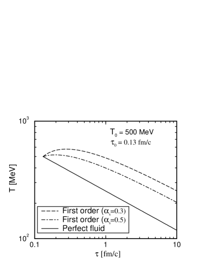
FIG. 4.: The $\tau$ dependence of temperature $T$, entropy density $s$ and the inverse of Reynolds number $R^{-1}$ in the scaling solution with $s$ and $\eta$ are proportional to $T^{3}$.

In Fig. 4 the $\tau$ dependence of $T,s,$ and $R^{-1}$ with two typical values of $\alpha_{s}$ is compared with the perfect fluid case. For both values of $\alpha_{s}$, $T,s$ and $R^{-1}$ have peaks, while for the perfect fluid they monotonically decrease and $R^{-1}$ monotonically decreases. In both cases the initial conditions are those determined from the uncertainty principle. This way of fixing initial conditions has a strong restriction on the value of the initial Reynolds number. It is seen in Fig. 5 that $R_{0}^{-1}$ will always be greater than one. This is the condition that gives rise to the peaks in temperature, energy density and entropy density. In the same Fig. 5 we also show the region for the condition $R_{0}>1$ in the $T_{0}\tau_{0}$–$\alpha_{s}$ plane for arbitrary initial conditions $(T_{0},\,\tau_{0})$ at a given $\alpha_{s}$.

The condition for decrease in the thermodynamical variables is

$$R_{0}\geq 1~{}~{}~{}~{}~{}\mbox{or}~{}~{}~{}~{}~{}T_{0}\tau_{0}\geq{1\over 3}{b\over a}\enspace,$$ (169)

where the initial Reynolds number can be calculated from

$$R=3{a\over b}T\tau\enspace.$$ (170)

The above condition and the initial conditions $\tau_{0}\approx 1/(3T_{0})$ implies $b\leq a$. It also determines the region where one might apply the Navier-Stokes-Fourier laws.

In (1+1) dimensions the (1+1)–dimensional scaling solution implies that the effective viscosity coefficient is only the bulk viscosity $\zeta$. This is also the case with the (3+1)–dimensional solution in (3+1) dimensions. This is due to the relation $\bigtriangledown^{\mu}u^{\nu}=\bigtriangleup^{\mu\nu}{\partial}_{\rho}u^{\rho}$ resulting from scaling solution. The (1+1)–dimensional scaling solution in (3+1) dimensions implies that the effective viscosity coefficient is ${4\eta/3}+\zeta$.

FIG. 5.: The $\alpha_{s}$ dependence of $R_{0}$ and the region which satisfies $R_{0}\geq 1$ is shown in the $\alpha_{s}$–$T_{0}\tau_{0}$ plane; where the curve is the condition $R_{0}=1$.

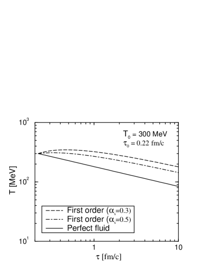
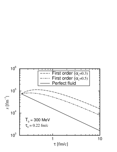
FIG. 6.: The $\tau$ dependence of temperature $T$ and entropy density $s$ for arbitrary initial conditions and for initial conditions from uncertainty principle.

In Fig. 6 we show how initial conditions affect the overall space–time evolution. In the top panel we show the results for arbitrarily chosen initial conditions. For this set of initial conditions dissipative effects are small. On the other hand the bottom panel with the initial conditions from uncertainty principle indicates that dissipative effects are significant.

B Causal Fluid Dynamics

We have seen in the previous section the importance of Reynolds’ number in determining the effects of dissipation. One of the mathematical advantages of the previous section is the direct connection between the Reynolds number and the initial conditions $(T_{0},\,\tau_{0})$. This is because the first order theory does not have well–defined initial conditions for the dissipative fluxes, and the latter are related to the thermodynamic forces by linear algebraic expressions.

In this section we determine the dissipative fluxes from the transport equations. In the Landau–Lifshitz frame the transport equations are still given by (74)–(76) but with slightly different heat coupling coefficients in the bulk and shear viscous pressure equations. Under the scaling solution assumption those coupling terms do not contribute to the dynamics of the system.

The $(1+1)$–scaling solution in $(3+1)$–dimensions yields the following structure of transport equations

$${{\partial}\Pi\over{\partial}\tau} = -{\Pi\over\tau_{\Pi}}-\frac{1}{2}{1\over\beta_{0}}\Pi\left[\beta_{0}{1\over\tau}+T{{\partial}\over{\partial}\tau}\left({\beta_{0}\over T}\right)\right]$$ (172)

$$-{1\over\beta_{0}}{1\over\tau}\enspace,$$

$${{\partial}q^{\mu}\over{\partial}\tau} = -{q^{\mu}\over\tau_{q}}+\frac{1}{2}{1\over\beta_{1}}q^{\mu}\left[\beta_{1}{1\over\tau}+T{{\partial}\over{\partial}\tau}\left({\beta_{1}\over T}\right)\right]\enspace,$$ (173)

$${{\partial}\pi^{\mu\nu}\over{\partial}\tau} = -{\pi^{\mu\nu}\over\tau_{\pi}}-\frac{1}{2}{1\over\beta_{2}}\pi^{\mu\nu}\left[\beta_{2}{1\over\tau}+T{{\partial}\over{\partial}\tau}\left({\beta_{2}\over T}\right)\right]$$ (175)

$$+{1\over\beta_{2}}\left[\tilde{\bigtriangleup}^{\mu\nu}-{1\over 3}\bigtriangleup^{\mu\nu}\right]{1\over\tau}\enspace.$$

In the last of the above equations $\tilde{\bigtriangleup}^{\mu\nu}=\bigtriangleup^{\mu\nu}$ for $0\leq\mu,\nu\leq 1$ and zero otherwise (because of only one non-vanishing spatial component of the 4–velocity).

For the (1+1)– dimensional Bjorken similarity fluid flow in (3+1) dimensions the energy equation (142) becomes

$$\frac{d\varepsilon}{d\tau}+\frac{\varepsilon+p}{\tau}-\frac{1}{\tau}\Phi+\Pi\frac{1}{\tau}=0\enspace,$$ (176)

where $\Phi\equiv\pi^{00}-\pi^{zz}$ is determined from the shear viscous tensor evolution equation (175)

$$\frac{d}{d\tau}\Phi = -\frac{1}{\tau_{\pi}}\Phi-\frac{1}{2}\Phi\left(\frac{1}{\tau}+\frac{1}{\beta_{2}}T\frac{d}{d\tau}\left(\frac{\beta_{2}}{T}\right)\right)+\frac{2}{3}\frac{1}{\beta_{2}}\frac{1}{\tau}\enspace.$$ (177)

The equation for $\Pi$ will not be needed because $\zeta=0$.

In this subsection we will distinguish the perfect fluid, first order, and second order theories by the quantity $\Phi$:

$$\Phi \equiv 0~{}~{}~{}~{}~{}~{}~{}~{}~{}~{}~{}~{}~{}~{}~{}\mbox{perfect fluid}\enspace,$$ (178)

$$\Phi = \frac{4}{3}\eta/\tau~{}~{}~{}~{}~{}~{}~{}~{}~{}~{}~{}~{}~{}~{}~{}\mbox{first order theory}\enspace,$$ (179)

$$\frac{d\,\Phi}{d\,\tau} = -{\Phi\over\tau_{\pi}}-{1\over 2}\Phi\left({1\over\tau}+{1\over\beta_{2}}T{d\over d\tau}\left({\beta_{2}\over T}\right)\right)+{2\over 3}{1\over\beta_{2}}{1\over\tau}$$ (181)

$$~{}~{}~{}~{}~{}~{}~{}~{}~{}~{}\mbox{second order theory}\enspace,$$

The Reynolds number is generally given by

$$R={(\varepsilon+p)\over\Phi}~{}~{}~{}~{}~{}\mbox{or}~{}~{}~{}~{}~{}{Ts\over\Phi}\enspace.$$ (182)

R goes to infinity in the ideal fluid approximation.

Let us first discuss the initial condition for $\Phi$. For an ideal fluid $\Phi$ vanishes since there are no dissipative fluxes. For the first order theories the initial condition for $\Phi$ is not well–defined and is given by the initial conditions $(T_{0},\,\tau_{0})$. For the second order theories we have well–defined initial condition for $\Phi$ since the dissipative fluxes are found from their evolution equations.

In deriving the transport equations it is assumed that the dissipative fluxes are small compared to the primary variables $(\varepsilon,\,n,\,p)$. For shear flux we require that

$$\left[\pi^{\mu\nu}\pi_{\mu\nu}\right]^{1/2}=\sqrt{{3\over 2}}\Phi\ll p\enspace.$$ (183)

In terms of $\Phi$ this condition can be written as

$$\Phi\ll\sqrt{{2\over 3}}p\enspace.$$ (184)

Another important quantity in determining the importance of viscous effects is the ratio of the macroscopic time scale to the microscopic time scale

$$R_{\tau}={\tau\over\tau_{\pi}(\tau)}\enspace,$$ (185)

which in our case is given by

$$R_{\tau}={2\over 3}{a\over b}T\tau\enspace.$$ (186)

In first order theories the question of how much a particular dissipative flux is generated as a response to corresponding thermodynamic/kinematic forces in nuclear collisions is governed by the primary initial conditions $(T_{0},\,\tau_{0})$. That is, one just reads off the value of $\Phi_{0}$ from the the linear algebraic expression for $\Phi$. We have seen that for values of the Reynolds number less than one, the thermodynamic quantities increase with time. This might be signalling the instability of the solution. Alternatively this might imply that we are using the first order theories beyond their domain of validity . The primary initial conditions can in principle be extracted from experiments. These in turn will give us the value of $\Phi_{0}$. This value of $\Phi_{0}$ will eventually determine how the thermodynamic variables evolve with time. This is clearly understood by looking at the ratio of the pressure term to viscous term, namely, $R$ as already discussed in the previous section.

In the second order theories the question of how much a particular dissipative flux is generated as a response to corresponding thermodynamic/kinematic forces in the early stages of nuclear reactions is not trivial but interesting. In order to find the viscous contribution to the time evolution of thermodynamic quantities we need to solve the differential equation for $\Phi$. Therefore one has to determine the initial conditions for $\Phi$. Although we don’t know the exact form of the initial value for $\Phi$ we will discuss the limiting cases. The first and most important limiting case is based on the assumption made when deriving the second order theory transport equations, namely, that the dissipative fluxes be small compared to the primary variables. For the shear viscous flux this means that the shear viscous stress–tensor must be small compared to the pressure. The value of $\Phi$ will always be less than $p$, hence the initial value $\Phi_{0}$ will always be less than $p_{0}$. This has an interesting consequence: the initial Reynolds number is always greater than one. Thus in second order theory under these conditions there will be no increase (and hence no peaks) of thermodynamic variables with increasing time. However in general the thermodynamic quantities will decrease with time for as long as the condition

$$\Phi\leq\varepsilon+p\enspace,$$ (187)

is satisfied, which in the present case implies that $\Phi_{0}\leq 4p_{0}$. However, values of $\Phi$ greater than the pressure $p$ leads to unphysical negative effective enthalpy. Unlike in the first order theories where it is not always possible to address this problem of negative effective enthalpy, in the second order theories we are guided by the limitations which are embedded in the valid application regimes of the theories, namely, the condition $(\pi^{\mu\nu}\pi_{\mu\nu})^{1/2}\ll p$. This condition guarantees that there effective enthalpy is always positive.

There are other two ways of determining the initial conditions for $\Phi$. The first one is by using the existing microscopic models such as VNI [40], (HIJING) [41] and (UrQMD) [42] to extract the various components of $\pi^{\mu\nu}$ from $T^{\mu\nu}$. Since we are dealing here with a partonic gas VNI seems to be a good choice for the present work. We will use the results from the improved version of VNI [46] to fit our calculation in order to extract the initial value for $\Phi$. Another way of determining the initial value for $\Phi$ is to extract the initial value of the Reynolds number experimentally. Two of the most experimentally accessible quantities are the multiplicity per unit rapidity ${\rm d}N/{\rm d}y$ and the transverse energy per unit rapidity ${\rm d}E_{T}/{\rm d}y$. A detailed study for the initial and boundary conditions for dissipative fluxes is needed to fully incorporate these fluxes into the dynamical equations for the thermodynamic quantities.

In this section we focus mainly on the results of second order theories and compare them to the first order theories and the perfect fluid results. As it is the main focus of this work we will look at the dynamics of the quark–gluon plasma or partonic gas.

The energy equation (176) and the viscous stress equation (177) can be written as

$$\frac{d}{d\tau}T = -\frac{T}{3\,\tau}+\frac{T^{-3}\Phi}{12\,a\,\tau}\enspace,$$ (188)

$$\frac{d}{d\tau}\Phi = -\frac{2\,a\,T\Phi}{3\,b}-\frac{1}{2}\Phi\left(\frac{1}{\tau}-5\frac{1}{T}\frac{d}{d\tau}T\right)+\frac{8\,a\,T^{4}}{9\,\tau}\enspace.$$ (189)

For a perfect fluid and a first order theory the energy equation (188) can be solved analytically to give (134) and (163) In the first order theory we do not have any relaxation coefficients. Then equation (177) gives $\Phi=(4\eta/3)/\tau$. Eqs. (134), (163) and the numerical solution to the second order equations (188) and (189) will be used to study the proper time evolution of temperature. The other thermodynamic quantities, namely, energy density and entropy density, are related to the temperature by the equation of state. It is important to show the entropy results due to the importance of entropy in the theory of irreversible extended thermodynamics and due to the fact that entropy is related to multiplicity.

We start by showing the dependence of the temperature evolution on the initial value of $\Phi$. In Fig. 7 we show this dependence for two values of $\alpha_{s}$. The dependence of first order results on $\alpha_{s}$ is clear from the results presented before. The dependence of the second order theory on $\alpha_{s}$ is different. A large value of $\alpha_{s}$ modifies the power dependence for $\tau\mbox{~{}{\raisebox{1.72218pt}{$>$}} {\raisebox{-2.58334pt}{$\sim$}}~{}}1$ fm/c to be more or less the same as the power dependence for $\tau\mbox{~{}{\raisebox{1.72218pt}{$<$}} {\raisebox{-2.58334pt}{$\sim$}}~{}}1$ fm/c. Thus the effect of $\alpha_{s}$ are important for $\tau>1$ fm/c as can be seen from the top right panel of Fig. 7 where a large value of $\alpha_{s}$ is shown.

In studying the dependence of the results on the initial conditions for $\Phi$ we have also included some unphysical choices for illustrative purposes. For $0.1<\Phi_{0}/p_{0}<1$ the choice of $\Phi_{0}$ is important, but below $\Phi_{0}=0.1p_{0}$ the equation for $\Phi$ gives the same contribution to the evolution of thermodynamic quantities.

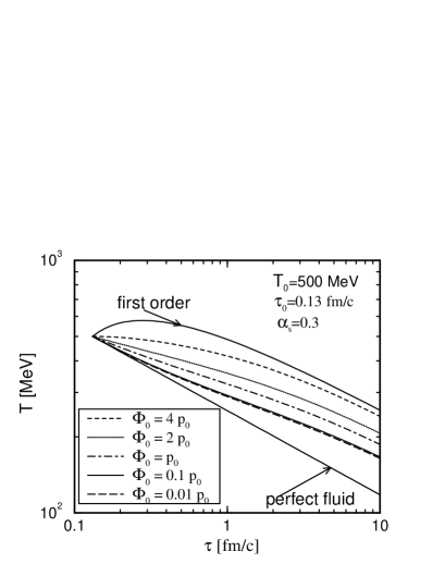
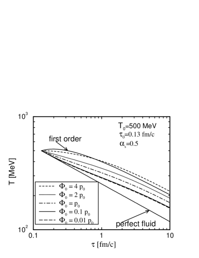
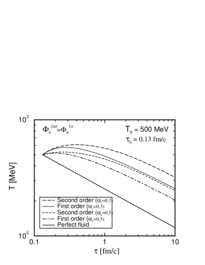
FIG. 7.: The time evolution of temperature for different choices of $\Phi_{0}$ for given primary initial conditions $(T_{0},\,\tau_{0})$, and two different values of $\alpha_{s}$. The curves for different values of $\Phi_{0}$ are from the second order theory. The bottom panel is for $\Phi_{0}^{2nd}=\Phi_{0}^{1st}$.

It is also tempting to choose the initial conditions for the second order theory to match what the first order theory predicts to be the initial value of $\Phi$. Note the order of the curves on the bottom panel of Fig. 7 . The second order theory predicts larger deviations than the first order theory. This should be exactly the same picture if both theories are synchronized in a regime where both are valid. Unfortunately, it is not trivial to make the reverse match of initial conditions. This situation will arise in natural way when both first order theory and second order theories are applied in the situation where they are both valid, as we will see later.

Under physical initial conditions the second order theory gives a Reynolds number that is always greater than one. This can be seen from Fig. 8 where for illustrative purposes we also include curves for unphysical initial conditions for $\Phi$. Note that $\Phi_{0}=4p_{0}$ is the maximum value before the solutions becomes unstable. This is a critical value that gives a Reynolds number $R_{0}=1$. As expected the first order theory gives $R<1$ at the same time. Throughout this work, unless otherwise stated so, we use the primary initial conditions based on the uncertainty principle as already discussed and as we will briefly describe below. Under this prescription of primary initial conditions, which might be relevant for RHIC and LHC, the first order theories are not suitable in describing the dynamics of thermodynamic quantities. On the other hand, the second order theories are suitable in describing the physical process happening at earlier times. An advantage of the extended irreversible thermodynamics, or second order theories, are their ability to be applicable over a wide range of regimes. However, for a different choice of initial conditions both theories might yield similar results, as we shall see.

FIG. 8.: Proper time evolution of the inverse Reynolds number for different values of $\Phi_{0}$ for the given primary initial conditions.

In what follows we will try to get close to the conditions that are realized in the laboratory. We will consider scenarios close to those at RHIC and LHC. We will use the most common primary initial conditions as discussed below. But first, we have to estimate the initial value of $\Phi$ for these two scenarios. We will use the recent results from VNI calculations for the proper time evolution [46]. We will make a fit to the data points and extract the initial value of $\Phi$.

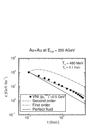
FIG. 9.: The proper time evolution of energy density. The data points are results from VNI simulations and the curves are fits.

Even though the motive is to extract an initial condition for $\Phi$, there is something interesting in Fig. 9. In this figure a comparison between the perfect fluid approximation, the first order theory, and the second order theory is clear. The kinetic theory result, of course, differs significantly from the perfect fluid dynamics result. The first order theory obviously fails terribly. The essential point, however, is that the second order theory is in good agreement with the VNI results. Due to the preliminary nature of VNI results we cannot yet claim perfect agreement between the two approaches. However, the fact that both have similar power laws is striking. In the beginning it looks like $\tau^{-1}$ and then later on $\tau^{-4/3}$ for the VNI results. One expects that when the full three dimensional problem is studied within the fluid dynamical approach we might have even better agreement. The fitted value of $\Phi_{0}$ is found to be about $0.2p_{0}$ which is, of course, a physical value. The value of $\alpha_{s}$ used is about $0.5$. For all RHIC results presented here we will use the expected primary initial conditions with $\Phi=0.2p_{0}$ and $\alpha_{s}=0.5$. For the LHC scenario we will use the expected primary initial conditions with $\Phi_{0}=0.3p_{0}$ and $\alpha_{s}=0.4$.

As a benchmark both the fluid dynamical and cascade models have been solved numerically for same primary initial conditions and equation of state. This is done for consistency. It is apparent that hyperbolic models performs better than the parabolic ones, in agreement with VNIBMS simulations. Also for energy density there is a peak in the parabolic model which is absent in hyperbolic model. This spurious unphysical result highlights the difference between the parabolic and hyperbolic model in region of large gradients. We remark that the initial state under consideration presents very steep velocity gradients. Therefore this is an ideal benchmark for testing fluid dynamical models against transport models. Comparisons of Navier–Stokes–Fourier results with transport models were made in [47] with NSF failing terribly for smaller cross sections. In that particular study the NSF also brought in the problem of negative effective pressure. The transport results however gave a much better description. What is important however is that the second order theory seems to do a better job even in this case. The latest results on this latter point to be published elsewhere are still under investigation and comparison to previous work on the effective pressure of a saturated Gluon plasma [48] is done.

The initial temperatures expected are $T_{0}$=500 MeV at RHIC and $T_{0}$=1000 MeV at LHC. In Figs. 10 and 11 the initial time $\tau_{0}$ is estimated by using the uncertainty principle [43]: $\tau_{0}\cdot{\langle E\rangle}_{0}\sim 1$ where ${\langle E\rangle}_{0}\sim 3T_{0}$ for massless particles. This results in $\tau_{0}$=0.13 fm/c at RHIC and $\tau_{0}$=0.07 fm/c at LHC. The initial value used for $\Phi$, must be specified independently for the second order theory. These values are legitimate since the second order theory is based on the assumption that the dissipative fluxes are small compared to the primary thermodynamic variables, namely $p,n,$ and $\varepsilon$. The effect of dissipation is more pronounced at the very early stages of heavy ion collisions when gradients of temperature, velocity, etc., are large. This can be seen by comparing Figs. 10, 11 with Fig. 12. At late times the effect of dissipation diminishes greatly. For comparison, in Fig. 12 we take a constant initial time $\tau_{0}$=1.0 fm/c, which is the characteristic hadronic time scale. From Figs. 10 and 11 Euler hydrodynamics predicts the fastest cooling. At hadronization times of order of 4 fm/c the perfect fluid dynamics solution decreases by a factor of about three. The first order theory fails badly even for this case where we have a very high initial parton density. The first order theory significantly under-predicts the work done during the expansion relative to the Müller-Israel-Stewart and Euler predictions. Thus the temperature decreases more slowly with the inclusion of dissipative effects. This would lead to greater yields of photons and dileptons. Also, the transverse energy and momentum would be reduced as the collective velocities are dissipated into heat. The system takes longer to cool down. This will delay freeze–out. The entropy, $s=4\,a\,T^{3}$, is enhanced. This is important because entropy production can be related to the final multiplicity.

A legitimate question to ask is: Do we really want to synchronize the initial conditions for both ideal fluid, first order and second order theories? Given some initial conditions we want to investigate the importance of second order theories as compared to first order theories and perfect fluids. That is, if one is given a set of well known initial conditions from experiment we want to see which of the theories best describe the dynamics of the system. Given an observable and a set of primary initial conditions we would like to see whether the microscopic cascade models, the ideal fluid, the first order theory or second order theory best describes the evolution of the system.

Let us now analyze the differences between the second order and first order theories. The first thing we notice is that the Eckart–Landau–Lifshitz theory predicts that at early times the temperature will rise before falling off. This is more pronounced when we have small initial times. Naively one would expect that the system would cool monotonically as it expands, even in the case of dissipation where energy-momentum is conserved. On the other hand, it is seen that for large initial times and high temperatures the three theories have a similar time evolution. As can be seen from Fig. 12, all three cases start at the same point and then fall off with time. The difference stems from the fact that in the second order theory the transport equations of the dissipative fluxes describe the evolution of these fluxes from an arbitrary initial state to an equilibrium state. The first order theory, though, is just related to the thermodynamic forces which, if switched off, do not demonstrate relaxation. Hence they are sometimes referred to as quasi–stationary theories. As can be seen from Fig. 12, it is before the establishment of an equilibrium state that the two theories differ significantly.

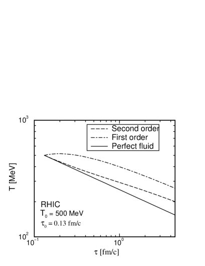
FIG. 10.: The proper time evolution of temperature and entropy for given primary initial conditions $(T_{0},\,\tau_{0})$ for a RHIC scenario.

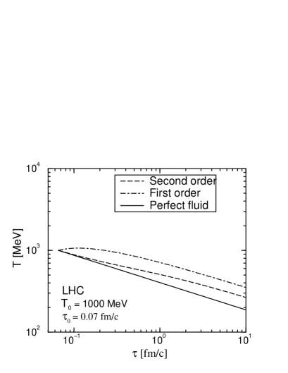
FIG. 11.: The proper time evolution of temperature and entropy for given primary initial conditions $(T_{0},\,\tau_{0})$ for LHC scenario.

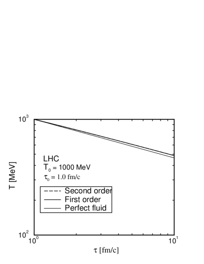
FIG. 12.: The proper time evolution of temperature for RHIC scenario and LHC scenario. The initial time is arbitrarily chosen. The first order and second order theories overlaps.

C Hadronic Fluid Dynamics

So far our focus has been on the quark–gluon plasma where the composition of the parton fluid enters the description through the form of the conservation laws and the equation of state. Now we study the dynamics of a pion fluid. Pions are the lightest hadrons. They are produced in abundance in ultra–relativistic collisions compared to heavier hadrons, particularly in the central region. It is therefore important to study their influence on the expansion. If pions are produced by hadronization of quark–gluon plasma, then dissipation encountered during their subsequent expansion may change the observables. The expansion in the central region conserves pion energy and momentum. Since pions carry baryon number zero, their total number is not conserved. Therefore, we expect the equilibrium number density of pions in a given volume to vary with temperature.

The equation of state is approximated by that of a massless pion gas. Thus the pressure is given by $p=a\,T^{4}$ with $a=g_{h}\pi^{2}/90$ where $g_{h}=3$ is the number of degrees of freedom. The energy density and entropy density are given by $\varepsilon=3\,a\,T^{4}$ and $s=4\,a\,T^{3}$ respectively. The bulk viscous pressure equation does not contribute for massless particles, since $\zeta\longrightarrow 0$ [36]. For the (1+1)–dimensional Bjorken-type hydrodynamics the heat term in the energy equation will not contribute. Thus we need only the shear viscous pressure for this presentation. The energy density evolution equation is determined by

$$\frac{d\,\varepsilon}{d\,\tau}=-\frac{(\varepsilon+p)}{\tau}+\frac{\Phi}{\tau}\enspace,$$ (190)

where

$$\Phi \equiv 0~{}~{}~{}~{}~{}~{}~{}~{}~{}~{}~{}~{}~{}~{}~{}\mbox{perfect fluid}\enspace,$$ (191)

$$\Phi = \displaystyle\frac{4}{3}\eta/\tau~{}~{}~{}~{}~{}~{}~{}~{}~{}~{}\mbox{standard theory}\enspace,$$ (192)

$$\tau_{\pi}\frac{d\,\Phi}{d\,\tau} = \displaystyle-\Phi-{1\over 2}\Phi\tau_{\pi}\left({1\over\tau}+{1\over\beta_{2}}T{d\over d\tau}\left({\beta_{2}\over T}\right)\right)+\frac{4}{3}\eta/\tau$$ (194)

$$~{}~{}~{}~{}~{}~{}~{}~{}~{}~{}~{}~{}~{}~{}~{}\mbox{extended theory}\enspace,$$

where $\eta=\tau_{\pi}/(2\beta_{2})$. For massless particles $\beta_{2}=3/(4\,p)$, and this is used in the expression for $\tau_{\pi}$. The primary transport coefficients of a massless pion gas are not that well-known. For chiral pions the expressions for shear viscosity and thermal conductivity are given in [26]. We will estimate the shear viscosity from the mean collision time of the pions. The mean time between collisions of pions moving at $\langle v\rangle\approx 1$ is given by

$$\tau_{\pi}={1\over\sigma n}\enspace,$$ (195)

where $n(T)=bT^{3}$ with $b=3\zeta(3)/\pi^{2}$ is the pion density and $\sigma\approx 1$ fm² is an effective cross section. The quantity $\tau_{\pi}T^{3}=1/(\sigma b)$ fm² is roughly constant for temperatures $T>100$ MeV. The shear viscosity can therefore be represented by

$$\eta=f_{\eta}T~{}~{}~{}~{}~{}\mbox{with}~{}~{}~{}~{}~{}f_{\eta}={2\over 3}{a\over b}{1\over\sigma}\enspace.$$ (196)

Using the transport and thermodynamic properties outlined here the energy and transport equations can be written as

$${{\rm d}T\over{\rm d}\tau} = -{1\over 3}{T\over\tau}+{1\over 12}{1\over aT^{3}\tau}\Phi\enspace,$$ (197)

$${{\rm d}\Phi\over{\rm d}\tau} = -\sigma bT^{3}\Phi-{1\over 2}\left({1\over\tau}-5{1\over T}{{\rm d}T\over{\rm d}\tau}\right)+{8\over 9}{aT^{4}\over\tau}\enspace.$$ (198)

The energy equation can be solved analytically for the perfect fluid and the first order (provided $\eta$ is constant) cases. But since we want $\eta$ to depend on temperature or time one must then solve the equations numerically, or first find the temperature evolution as done in the previous section. In the case of the perfect fluid and the first order theories the energy equation is readily solved.

$$T(\tau) = T_{0}\left[\tau_{0}\over\tau\right]^{1/3}~{}~{}~{}~{}~{}~{}~{}~{}~{}~{}\mbox{perfect fluid}\enspace,$$ (199)

$$T(\tau) = T_{0}\left[\tau_{0}\over\tau\right]^{1/3}\left\{1+{f_{\eta}\over 3aT_{0}^{3}\tau_{0}}\ln\left[\tau_{0}\over\tau\right]\right\}^{1/3}~{}~{}~{}~{}~{}\mbox{first order}\enspace.$$ (200)

Hydrodynamics applies to the intermediate stages of the evolution until the system eventually freezes out of local equilibrium into freely streaming fragments as it expands. At freeze–out hydrodynamics must break down, since the pion collision rate drops below the local expansion rate. The system will be purely longitudinal as long as its transverse motion can be neglected. Once the transverse rarefaction wave reaches the center, however, the flow becomes effectively three dimensional, so that the density diminishes as $\tau^{-3}$. Freeze out then occurs because the mean free path, which then increases as $\tau^{3}$, grows faster than the expansion time scale $\mid n/\dot{n}\mid=\tau/3$.

In Fig. 13 we show the $\tau$ dependence of temperature for the three different cases: a perfect fluid, a first order theory of dissipative fluids and a second order theory of dissipative fluids. Here we assume that the pion gas is produced at hadronization of quark–gluon plasma at $\tau=4$ fm/c. As expected, in this regime, with the given initial conditions, the first order and second order theories converge. This convergence is faster with increasing cross sections. The effects of viscosity are small but non–negligible.

FIG. 13.: The proper time evolution of temperature for or $\sigma=1.0$ fm² and $\sigma=3.0$ fm². The initial conditions ($T_{0},\,\tau_{0}$) are arbitrarily chosen. The first order and second order theories overlaps.

In Fig. 14 we assume that the pion gas is formed at $\tau_{0}\sim 1/(3T_{0})$. As we know by now, the difference between the three theories is noticeable and first order theories are not suitable. We see here also that the convergence of first order theory results and second order theory results will occur for large cross sections.

FIG. 14.: The proper time evolution of temperature for $\sigma=1.0$ fm² and $\sigma=3.0$ fm². The primary initial conditions are those from uncertainty principle.

The presence of dissipation in heavy ion reactions will have profound effects on the space–time evolution of the system. The freeze–out will be delayed. Temperature and energy density decrease more slowly. Enhancement of entropy production will increase the production of observed particles since the two can be related. Since the system takes longer to cool this will lead to an enhancement in the production of thermal signals (dileptons and photons).

VII Conclusions

In this work I have given a comprehensive exposition of the non–equilibrium properties of a new state of matter produced in heavy ion reactions. In doing so I presented some basic features of non–equilibrium fluid dynamics. I studied the space–time description of high energy nuclear collisions. I chose to follow the phenomenological approach and left kinetic theory approach for future work.

The ultimate aim is to bridge the phenomenological theory with the kinetic theory of the matter produced in heavy ion coliisions. In doing so I made use of the dissipative fluid dynamics. The connection between the macroscopic theory and microscopic theory enters through the transport coefficients of the matter. The equation of state provided closure to the system of conservation equations.

I demonstrated that extended irreversible thermodynamics provides a consistent framework to simulate and study the space–time evolution of ultra-relativistic nuclear collisions, from some initial time to the final particle yield. Although this approach relies on a number of fundamental assumptions and is far from providing an accurate quantitative description, it has the advantage of wide applicability.

The advent of accelerators such as RHIC and LHC provide an opportunity for studying the dynamics and properties of the matter at very high energy density. In the description of the evolution of such a system, it is mandatory to evaluate, as accurately as possible, the order of magnitude of different characteristic time scales, since their relationship with the time scale of observation will determine, along with the relevant equations, the evolution pattern. This is rather general when dealing with dissipative systems. It has been my purpose here, by means of simple model with simple equation of state and arguments related to a wide range of time scales, to emphasize the convenience of resorting to hyperbolic theories when dissipative processes, either outside the steady–state regime or when the observation time is of the order of or shorter than some characteristic time of the system, are under consideration. Furthermore, dissipative processes may affect the way in which the system tends to equilibrium, thereby affecting the future of the system even for time scales much larger than the relaxation time.

In the early stages of heavy ion collisions, non–equilibrium effects play a dominant role. A complete description of the dynamics of heavy ion reactions needs to include the effects of dissipation through dissipative or non–equilibrium fluid dynamics. As is well–known, hyperbolic theories of fluid dissipation were formulated to get rid of some of the undesirable features of parabolic theories, such as acausality. It seems appropriate therefore to resort to hyperbolic theories instead of parabolic theories in describing the dynamics of heavy ion collisions. Thus in ultra–relativistic heavy ion collisions, where the fluid evolution occurs very rapidly, the second order theories, due to their universality, should be used to analyze collision dynamics.

Unlike in first order theories, where the transport equations are just the algebraic relations between the dissipative fluxes and the thermodynamic forces, second order theories describe the evolution of the dissipative fluxes from an arbitrary initial state to a final steady-state using the transport equations. The presence of relaxation terms in second order theories makes the structure of the resulting transport equations hyperbolic and they thus represent a well-posed initial value problem.

The consequences of non-ideal fluid dynamics, both first order (if applicable) and second order were demonstrated here in a simple situation, that of scaling solution assumption and simple equation of state. A more careful study of the effects of the non-ideal fluid dynamics on the observables is therefore important. Conversely, measurements of the observables related to thermodynamic quantities would allow us to determine the importance and strength of dissipative processes in heavy ion collisions.

Here we have used only a simple equation of state in a simplified model of high energy nuclear collisions. A more realistic situation (including transverse expansion) will require careful analysis of both the transport coefficients and the equation of state which are employed in the full set of the equations. It is then that one may have a better understanding of when to use either of these theories in the context of relativistic heavy ion collisions.

A The Need for Hyperbolic Theories of Relativistic Dissipative Fluid Dynamics for Nuclear Collisions

The need for hyperbolic theories of dissipative fluid dynamics has been emphasized before [53]. But it is in ultra–relativistic nuclear collisions where it needs to be stressed.

The first order theories of dissipative fluid dynamics have a long history and proved very useful, in some special cases in understanding observables. However, they exhibit some undesirable features, such as acausality, that prompted the formulation of hyperbolic theories of dissipative fluid dynamics to get rid of them. This was achieved at the price of extending the set of field variables by including the dissipative fluxes, such as the heat current and viscous stresses, on the same footing as the primary ones, such as energy densities, equilibrium pressures, and number densities, thereby giving rise to a set of more physically satisfactory but involved theories from the mathematical point of view. These theories have the additional advantage of being backed by a kinetic theory of gases (Grad’s 14–moment approximation). Second order theories, being hyperbolic in structure, lead to well-posed initial-value (Cauchy) problems. They also lead to causal propagation. Unlike the first order theories, second order theories have relaxation terms which permit us to study the evolution of the dissipative fluxes.

In addition to causality violation, the Eckart theory leads to unstable equilibrium states under small perturbations. A dissipative hot and dense nuclear matter may very rapidly tend towards a quasi–stationary state that is adequately described by the Eckart theory. However, this needs to be checked a priori. The Eckart theory can describe steady–state regimes. However it is clearly unable to deal with the evolution towards these regimes, or with the overall dynamics of the fluid, in a satisfactory way.

It can be argued that the infinite speeds of propagation predicted by parabolic theories and the unphysical behaviour of the space–time evolution of thermodynamic quantities is just a consequence of using them outside their range of applicability [14]. However hyperbolic theories also share this constraint but they naturally predict speeds which are of the order of the characteristic speeds of the problem at hand. Therefore hyperbolic theories have a much wider range of applicability than parabolic theories.

Aside from the relaxation time $\tau$, hyperbolic theories introduce a certain number of new coefficients that couple the different dissipative fluxes. This is rather natural, since these theories are designed to explain more complex phenomena than parabolic theories do. These quantities are not free parameters that one could choose at will. These new coefficients are restricted by the convexity of the entropy function, and can be calculated explicitly with the help of kinetic theory or fluctuation theory. It turns out that they are functions of the equation of state.

In summary, although parabolic theories have proved very useful for many practical purposes, they appear to fail hopelessly in describing the dynamics of heavy ion collisions. In contrast, hyperbolic theories successfully give a better description in agreement with transport models and hopefully they will be able to predict the experimental results. Thus hyperbolic theories are more reliable. In the steady–state, under the conditions mentioned before, and for times exceeding $\tau$ both theories converge. Based on the results presented here one can only stress the convenience of using hyperbolic transport equations when parabolic theories either fail or the problem under consideration happens to lie outside the range of applicability of parabolic theories.

I will conclude by pointing out some of the advantages and challenges of the second order theories. The challenge we face is the increase in the space of thermodynamic variables. We now have, in addition to the transport coefficients, new coefficients in the problem. These are the relaxation coefficients $\beta_{i}$ and the coupling coefficients $\alpha_{i}$. These new coefficients depend on the primary thermodynamic variables, such as $n,\varepsilon$ and $p$ and therefore are determined by the equation of state. Like viscosity and thermal conductivity, which are required to be positive by the second law of thermodynamics, these new coefficients are constrained by hyperbolicity requirements. In principle , in order to solve the second order relativistic dissipative fluid dynamic problem, one still needs the equation of state, initial conditions and the transport coefficients. Another challenge involves solving the equations numerically. Finally one would like to compare the results of non–equilibrium fluid dynamics to observables. This will require an effort to solve the full system of equations numerically. Efforts in this direction are under way [54]

The study of non-ideal or non–equilibrium fluid dynamics will be important for constructing hydro-molecular dynamic schemes [49]. Hyperbolic theories might prove to be convenient in such scheme. A resulting hydro-molecular dynamic scheme can then be compared to the studies of multi-fluid dynamics [50].

VIII Outlook

There are important questions that need to be investigated in order to tackle the challenges faced by hyperbolic theories. An important question is the measurability of the dissipative fluxes. The heat flux through a system may be simply evaluated by measuring the amount of energy transported per unit area and time. The viscous pressure can be measured from the tangential shear force exerted per unit area. In practice, it may be difficult to evaluate these quantities at each instant and at every point. From kinetic theory these fluxes can be simulated from microscopic transport models such as HIJING, VNI and UrQMD.

A thorough study of transport coefficients is needed. The results from lattice QCD should give clear predictions for these coefficients. So far there are no reliable phenomenological expressions for the coefficients. The shear viscosity results presented in [55] using the microscopic model UrQMD serve as a starting point for future calculations of transport coefficients.

A thorough study of the equation of state is required in order to be consistent with the non–equilibrium description of matter. In addition to the initial/boundary conditions for the primary/equilibrium variables a thorough study of initial/boundary conditions for the dissipative fluxes is necessary. This is required for the evolution equations of the fluxes. For example, one would like to know how much of a particular dissipative flux is generated as a response to an associated thermodynamics force in the early stages of the heavy ion collisions. This in turn gives us information about the initial entropy generated as a result of dissipation.

For the complete description of the dynamics of viscous, heat conducting matter we need to consider more realistic situations: a system that expands in both the longitudinal and transverse directions [54] and we need a full (3+1)–dimensional solutions to the conservation and evolution equations. This will require extensive numerical computation. This is a challenging but interesting problem. In order to understand the observables we need a full formulation of hyperbolic theory that should be tested against other models/theories.

To solve imperfect hydrodynamics amounts to knowledge of (i) a realistic equation of state, (ii) reliable transport coefficients (ii) realistic initial/boundary conditions and (iv) numerical computational algorithm. In order to understand the observables from RHIC and LHC knowledge of these requirements is needed and that is what I have started to do. I hope that this will gather momentum in due course.