Gamow-Teller transitions and deformation in the proton-neutron random phase approximation

Abstract

We investigate reliability of Gamow-Teller transition strengths computed in the proton-neutron random phase approximation, comparing with exact results from diagonalization in full $0\hbar\omega$ shell-model spaces. By allowing the Hartree-Fock state to be deformed, we obtain good results for a wide variety of nuclides, even though we do not project onto good angular momentum. We suggest that deformation is as important or more so than pairing for Gamow-Teller transitions.

I Introduction

Weak processes, such as beta ($\beta$) and double-beta ($\beta\beta$) decay, have deep consequences for nucleosynthesis LMP03 and physics beyond the Standard Model Zde02 . Weak processes are also sensitive to details of nuclear structure: allowed Gamow-Teller (GT) transitions depend in particular upon Pauli blocking LMP03 ; AZZ93 . Thus, predictions for astrophysics as well as interpretation of $\beta\beta$-decay experiments must be modeled with care. Because of this sensitivity to Pauli blocking and thus upon configuration mixing, the large-basis interacting shell model (SM) BW88 provides one of the best microscopic approaches to Gamow-Teller transitions.

The interacting shell model, however, is computationally expensive, and only recently has the full $0\hbar\omega\,\,pf$-shell become tractable. A simpler approach is the random phase approximation (RPA) and its generalizations, which have been widely and successfully applied to giant resonances such as the electric dipole (giant dipole resonance or GDR) Goeke82 , and has also been applied to many important problems in weak transitions LMP03 ; jameel ; c12rpa ; 2betarpa ; ZB93 ; engel1997 . It is not immediately obvious, however, that the RPA is an appropriate approximation for all transitions. Because the RPA is the small-amplitude limit of time-dependent mean-field theory Rowe70 ; ring , it seems appropriate for the GDR, which can be described semiclassically in the Goldhaber-Teller model GT48 as protons oscillating in bulk against neutrons. The application of the RPA and its extensions to Gamow-Teller transitions, although with a long history KS63 ; pnQRPA , is more problematic. Two implicit assumptions in the RPA are, first, ground-state correlations on top of a mean-field state are small, and, second, particle-hole phonons have boson commutation rules, which means that Pauli blocking is not fully treated. Therefore, as GT transitions are sensitive to Pauli blocking, they may not be well matched to RPA calculations.

Reading the literature only furthers these doubts. A number of authors have previously tested the efficacy of calculating GT transitions within the proton-neutron quasiparticle RPA (pnQRPA), through comparison with exact calculations either with full shell-model diagonalization Lau88 ; CMS91 ; ZB93 ; ABB93 or group-theoretical schematic models engel1997 . The efficacy of these pnQRPA calculations, which we will discuss in more detail below, can be broadly summarized as poor, typically overestimating the total transition strength and underestimating the first moment of the transition strength. In order to compare with the calculations described below, is important to understand that these calculations used spherical $J=0$, $N$-even $Z$-even parent states and treated pairing carefully, starting with either the Hartree-Fock-Bogoliubov or the Bardeen-Cooper-Schrieffer equations.

With the exception of those tests of Gamow-Teller transitions, however, most other tests of the RPA and its generalizations have been against toy models. Recently we began to systematically test the RPA against full shell-model diagonalization stetcu2002 ; johnson2002 ; stetcu2003 . In this paper we describe the generalization to proton-neutron RPA (pnRPA) and compare Gamow-Teller transitions against the full shell-model results. In contrast to previous approaches, we do not treat pairing carefully, but do allow arbitrary deformation, even though we do not project to good angular momentum. Furthermore we are not limited to even-even nuclides. We obtain good transition strengths, and where we can compare to published spherical pnQRPA strengths, our calculations are generally superior. We therefore conclude that proper treatment of deformation, even without projection, is at least as important as proper treatment of pairing, and arguably more so. This agrees with shell model studies that show a correlation between E2 transition strengths (a measure of deformation) and GT transition strengths AZZ93 ; TDH96 .

We also briefly argue that the pnRPA frequencies should be real, and not complex; such an argument is missing from the literature. Included in this discussion is a lemma helpful to understanding the solution of the pnRPA eigenvalue equations.

II Formalism

In this paper we consider only change-changing Gamow-Teller transitions; the transition operators are thus:

$${\cal O}_{\pm}=g_{A}\vec{\sigma}\tau_{\pm},$$ (1)

where $\tau_{+}$ changes a neutron into a proton. Because here we consider only strength distributions and not absolute transition strengths, we drop the axial vector coupling $g_{A}$. The transition strength from the parent state $|i\rangle$ (here always a ground state) to a final state $f$ at excitation energy $E=E_{f}-E_{i}$ is given by

$$S(E)=\sum_{f}\delta(E_{f}-E_{i}-E)\left|\left\langle f\right|{\cal O}\left|i\right\rangle\right|^{2}.$$ (2)

The transition strength to a given level is also often called the B(GT) value.

A convenient way to characterize the distribution of transition strength is through moments. The zeroth moment is the total transition strength, $S_{0}$,

$$S_{0}=\sum_{E}S(E),$$ (3)

while the centroid of the distribution $\bar{E}$ is the first moment

$$\bar{E}=\sum_{E}E\,S(E)/S_{0}$$ (4)

(note that this centroid is relative to the parent energy $E_{i}$) and the width of the distribution, $\Delta E$, is the square root of the second moment, calculated relative to the centroid:

$$\Delta E^{2}=\sum_{E}(E-\bar{E})^{2}S(E)/S_{0}.$$ (5)

An important check of any calculation is the well-known Ikeda sum rule, which holds true for any parent state, both in the SM and in the RPA:

$$S_{0}(\beta^{-})-S_{0}(\beta^{+})=3(N-Z).$$ (6)

We now briefly review the random phase approximation and its variant, the proton-neutron RPA (pnRPA) pnQRPA . Unlike the standard or like-particle RPA, pnRPA provides means to calculate excited states of neighboring isobars. The starting point, however, is similar to the regular RPA: a mean-field solution of the parent nucleus, which in turn defines a particle-hole basis. In our case we began with a Hartree-Fock state $|\mathrm{HF}\rangle$, allowing unrestricted deformation. The RPA can be derived a number of ways, but it essentially approximates the energy surface about the mean-field state as a harmonic oscillator. This leads to an RPA ground state $|\mathrm{RPA}\rangle$, which implicitly includes zero-point fluctuations about the mean-field state $|\mathrm{HF}\rangle$, and excited states are one-phonon excitations on the ground state:

$$|\lambda\rangle=\beta_{\lambda}^{\dagger}|\mathrm{RPA}\rangle.$$ (7)

For RPA one usually assumes the creation operators are simple one-particle, one-hole operators. In order to properly discuss the pnRPA, it is useful to further, if briefly, recapitulate the like-particle RPA ring . In the matrix formalism, one solves

$$\left(\begin{array}[]{cc}\mathbf{A}&\mathbf{B}\\ -\mathbf{B}&-\mathbf{A}\end{array}\right)\left(\begin{array}[]{c}\vec{X}\\ \vec{Y}\end{array}\right)=\Omega\left(\begin{array}[]{c}\vec{X}\\ \vec{Y}\end{array}\right)$$ (8)

Here the matrix $\mathbf{A}$, a Hermitian matrix, is in fact the submatrix of $H$ between one-particle, one-hole states (also the matrix for the Tamm-Dancoff approximation), while the elements of $\mathbf{B}$, a symmetric matrix, are the matrix elements of $H$ between the HF state and two-particle, two-hole states. (For simplicity we assume real HF wavefunctions so that all subsequent quantities are real.) One can show that the excitation frequencies $\Omega$ are real if the stability matrix,

$$\left(\begin{array}[]{cc}\mathbf{A}&\mathbf{B}\\ \mathbf{B}&\mathbf{A}\end{array}\right)$$ (9)

has no negative eigenvalues; this is equivalent to the Hartree-Fock state being at a (local) minimum. Part of the proof of this requires that both $\mathbf{A}\pm\mathbf{B}$ have no negative eigenvalues ring , which in turn requires that $\mathbf{A}$ have no negative eigenvalues. We emphasize this point because the situation will be different for pnRPA.

One can show that the solutions of Eq. (8) come in pairs: if $(\vec{X},\vec{Y})$ is a solution with frequency $\Omega$, then $(\vec{Y},\vec{X})$ is also a solution with frequency $-\Omega$. The solution with $\Omega>0$ is associated with the vector $(\vec{X},\vec{Y})$ such that $|X|>|Y|$, and one chooses a normalization $|X|^{2}-|Y|^{2}=1$; that one can do this also derives from the nonnegative eigenvalues of the stability matrix. The special case $\Omega=0$ corresponds to invariance of the Hamiltonian under a symmetry, for example, rotation or translation; here the vector $(\vec{X},\vec{Y})$ cannot be normalized, as $|X|=|Y|$, and one must resort to a different formalism ring ; stetcu2003 ; weneser .

The proton-neutron RPA is similar to the like-particle RPA but with important differences. For like-particle RPA, the phonon creation operator $\beta^{\dagger}$ uses one-particle, one-hole operators of the form $\pi^{\dagger}\pi$, $\nu^{\dagger}\nu$ (thus the name like-particle). The pnRPA phonon creation operator is also one-body but changes the third component of isospin $T_{z}$:

$$\beta^{\dagger}_{\lambda}=\sum_{mi}\left(X_{mi,\lambda}(pn)\pi^{\dagger}_{m}\nu_{i}-Y_{mi,\lambda}(np)\nu^{\dagger}_{i}\pi_{m}\right)+\sum_{mi}\left(X_{mi,\lambda}(np)\nu^{\dagger}_{m}\pi_{i}-Y_{mi,\lambda}(pn)\pi^{\dagger}_{i}\nu_{m}\right).$$ (10)

The first and the fourth terms in this equation describe the excited states of the $(Z+1,N-1)$ isobar, while the second and third the $(Z-1,N+1)$ isobar. We follow the standard convention and use indices $m,n$ for ‘particle’ states, that is, unfilled single-particle states in the Hartree-Fock wavefunction, and $i,j$ for ‘hole’ states, or filled single-particle states; thus $\pi^{\dagger}_{m}\nu_{i}$ destroys a filled neutron state (or creates a neutron hole in the HF wavefunction, in the usual view) and creates a proton in an excited particle state. The equation of motion

$$\langle\mathrm{RPA}|[[\delta\beta,[H,\beta^{\dagger}]]|\mathrm{RPA}\rangle=\Omega\langle\mathrm{RPA}|[\delta\beta,\beta^{\dagger}]|\mathrm{RPA}\rangle,$$ (11)

transforms as usual to a non-hermitian eigenvalue problem ring

$$\left(\begin{array}[]{cccc}A^{np,pn}&0&0&B^{np,pn}\\ 0&A^{pn,np}&B^{pn,np}&0\\ 0&-B^{np,pn}&-A^{np,pn}&0\\ -B^{pn,np}&0&0&-A^{pn,np}\end{array}\right)\left(\begin{array}[]{c}X(pn)\\ X(np)\\ Y(np)\\ Y(pn)\end{array}\right)=\Omega\left(\begin{array}[]{c}X(pn)\\ X(np)\\ Y(np)\\ Y(pn)\end{array}\right),$$ (12)

where the definitions for $A^{pn,np}$ and $B^{np,pn}$ matrices are similar to the regular proton-neutron conserving formalism, where one approximates $|\mathrm{RPA}\rangle\approx|\mathrm{HF}\rangle$:

$$A_{mi,nj}^{np,pn}=\langle{\rm HF}|[\nu_{i}^{\dagger}\pi_{m},[H,\pi_{n}^{\dagger}\nu_{j}]]|{\rm HF}\rangle=(\epsilon^{p}_{n}-\epsilon_{i}^{n})\delta_{mn}\delta_{ij}-V^{pn}_{mn,ji},$$ (13)

$$B_{mi,nj}^{np,pn}=-\langle{\rm HF}|[\nu_{m}^{\dagger}\pi_{i},[\pi_{n}^{\dagger}\nu_{j},H]]|{\rm HF}\rangle=-V_{in,jm}^{pn}.$$ (14)

(For the quasiparticle RPA (QRPA) one uses instead of the Hartee-Fock state a Hartree-Fock-Bogoliubov state or a Bardeen-Cooper-Schrieffer state, and the QRPA phonon is composed of quasiparticle-quasihole operators instead.) The matrices $A^{pn,np}$ and $B^{pn,np}$ are defined similarly, but are distinct unless $Z=N$; in fact, they have different dimensions unless $Z=N$. Let $N_{p}^{\pi}$, $N_{h}^{\pi}$ be number of proton particle and hole states, respectively, and $N_{p}^{\nu}$, $N_{h}^{\nu}$ the number of neutron particle and hole states. Thus the vectors $X(pn)$ and $Y(np)$ are of length $N_{p}^{\pi}N_{h}^{\nu}$ while vectors $X(np)$, $Y(pn)$ are of length $N_{p}^{\nu}N_{h}^{\pi}$; the two lengths are unequal unless $Z=N$. Similarly, $\mathbf{A}^{np,pn}$ is a square matrix of dimension $N_{p}^{\pi}N_{h}^{\nu}$ while $\mathbf{A}^{pn,np}$ is a square matrix of dimension $N_{p}^{\nu}N_{h}^{\pi}$, while $\mathbf{B}^{np,pn}$ is a rectangular matrix of dimension $N_{p}^{\pi}N_{h}^{\nu}\times N_{p}^{\nu}N_{h}^{\pi}$, and $\mathbf{B}^{pn,np}=\left(\mathbf{B}^{np,pn}\right)^{T}$ .

The zeroes in Eq. (12) occur because the original Hamiltonian conserves charge (and thus $T_{z}$). The overall form of Eq. (12) is identical to that of Eq. (8); we have merely introduced a block structure to $\mathbf{A}$, $\mathbf{B}$. Because of the zeroes in Eq. (12), the equations decouple:

$$\left(\begin{array}[]{cc}A^{np,pn}&B^{np,pn}\\ -B^{pn,np}&-A^{pn,np}\\ \end{array}\right)\left(\begin{array}[]{c}X(pn)\\ Y(pn)\end{array}\right)=\Omega\left(\begin{array}[]{c}X(pn)\\ Y(pn)\end{array}\right)$$ (15)

and

$$\left(\begin{array}[]{cc}A^{pn,np}&B^{pn,np}\\ -B^{np,pn}&-A^{np,pn}\\ \end{array}\right)\left(\begin{array}[]{c}X(np)\\ Y(np)\end{array}\right)=\Omega\left(\begin{array}[]{c}X(np)\\ Y(np)\end{array}\right)$$ (16)

It is important to note two things here. First, the decoupled equations (15) and (16) are not of the same form as Eq. (8), because $\mathbf{A}^{pn,np}\neq\mathbf{A}^{np,pn}$ unless $Z=N$. Because of this, some of the usual theorems do not immediately apply to (15) and (16), especially regarding the positivity of $\Omega$ (more about this, however, in a moment) and the sign of $|X|^{2}-|Y|^{2}$.

Second, any solution $(X(pn),Y(pn))$ to Eq. (15) with frequency $\Omega$ is related to a solution $(X(np),Y(np))$ of Eq. (16) with frequency $-\Omega$, by $(X(np),Y(np))=(Y(pn),X(pn))$, up to some overall phase factor. This simplifies finding solutions. Let $(U,V)$ be a solution of Eq. (15) with frequency $\omega$, which can be positive or negative. If $|U|^{2}-|V|^{2}>0$, and so normalizable to $1$, then let $(X(pn),Y(pn))=(U,V)$ with frequency $\Omega=\omega$. Otherwise, if $|U|^{2}-|V|^{2}<0$, then let $(X(np),Y(np))=(V,U)$ with frequency $\Omega=-\omega$ be the solution to Eq. (16). In both cases one can normalize to 1.

What about $\Omega=0$? In like-particle RPA, if exact symmetries are broken by the mean-field, one obtains zero eigenvalues; the corresponding eigenvectors, which identify the generators of the broken symmetries thouless61 , are not normalizable and must be treated with care. For pnRPA, although zero eigenvalues are not excluded, the corresponding eigenvectors do not play a special role and are in fact normalizable, as argued below.

In like-particle RPA, one can show that stability of the mean-field state implies that $\Omega\geq 0$. But now in pnRPA one can have $\Omega<0$, even for $|X|^{2}-|Y|^{2}=1$. At first glance this is troubling; however, we provide two arguments which resolve this apparent paradox.

First, because pnRPA allows charge-changing phonons of the form (10), one should, at least implicitly, also perform the Hartree-Fock minimization allowing mixing of proton and neutron states, with $N$-$Z$ fixed by a Lagrange multiplier $\lambda$. (We have in fact done such a calculation, but the results are indistinguishable from fixing $N$-$Z$ by hand, that is, as one varies $\lambda$, $N$-$Z$ makes integral jumps. Nonetheless, the image is useful.) Now the constrained Hartree-Fock is at a true minimum, and if one considers the eigenfrequencies of (12) all the resultant pnRPA frequencies are proven positive-definite (although in practice one solves (15) or (16) instead). To interpret the results as physical transition energies, however, one has to subtract off $\lambda(N-Z)$ which leads to negative frequencies.

One can see this directly. By adding the Langrange multiplier, one shifts the diagonals of the $\mathbf{A}$ matrices,

$$\tilde{A}^{np,pn}=A^{np,pn}-\lambda(N-Z)\cdot I,$$ (17)

and

$$\tilde{A}^{pn,np}=A^{pn,np}+\lambda(N-Z)\cdot I.$$ (18)

By substituting into Eq. (15), it is clear one is adding a constant along the entire diagonal, which only shifts $\Omega$ to $\tilde{\Omega}=\Omega+\lambda(N-Z)$, while the frequencies in Eq. (16) are shifted in the opposite direction. In fact, for any value of $\lambda$ one only shifts the frequencies and the solutions $(X,Y)$ are manifestly unchanged.

We call this result the shift lemma: by adding the Lagrange multiplier one shifts the relative position of the proton and neutron Fermi surfaces, but the only result is shifting the absolute value of the pnRPA frequencies. The relative frequencies and the eigenvectors are unchanged. There is a useful consequence: if one obtains a zero mode, from the shift lemma one can find a case where the frequency corresponding to the same eigenvector is positive, and one expects the pnRPA vector to be normalizable; and as the eigenvector is independent of the shift, it is always always normalizable. The reader should note that the shift lemma only arises because of the unique isospin dependence of the block decomposition (12); no such shift is possible for like-particle RPA because one cannot add a constant to the diagonal.

III Results

We test the reliability of pnRPA’s predictions for GT strengths against exact diagonalization in full $0\hbar\omega$ SM spaces. That is, we calculate the GT strength distributions for several nuclei in the $sd$ ($1s_{1/2}$-$0d_{3/2}$-$0d_{5/2}$) shell on top of an inert ¹⁶O core, and two Ti isotopes in the $pf$ ($1p_{1/2}$-$1p_{3/2}$-$0f_{5/2}$-$0f_{7/2}$) shell above a ⁴⁰Ca core. While we do not compare directly with experiment, we use in our calculations phenomenological interactions which are very successful in reproducing the experimental data: Wildenthal ‘USD’ in the $sd$ shell wildenthal , and Richter-Brown in the $pf$ shell RvJB91 . The shell model diagonalization were performed using a descendent of the Glasgow code Whitehead77 , and the shell-model strength distributions using an efficient Lanczos moment method LanczosMoment .

Having defined the pn-phonon creation operator $\beta^{\dagger}$ in (10), one can calculate the transition matrix element required by Eq. (2) as

$$\langle\mathrm{RPA}|{\cal O}|\lambda_{(Z\pm 1,N\mp 1)}\rangle=\langle\mathrm{RPA}|[{\cal O},\beta_{\lambda}^{\dagger}]|\mathrm{RPA}\rangle=\sum_{mi}\left(X_{mi}^{\lambda}(pn/np){\cal O}_{mi}+Y_{mi}^{\lambda}(pn/np){\cal O}_{im}\right).$$ (19)

In our case, ${\cal O}$ is the GT transition operator defined in (1), which induces transitions between the correlated ground state of the parent nucleus and the $(Z+1,N-1)$ or $(Z-1,N+1)$ isobars.

Table 1 summarizes results for total transition strengths, centroids and distribution widths, where indeed we find that the pnRPA moments are reasonably close to SM. As a check, note that the Ikeda sum rule (6) is fulfilled in both SM and pnRPA, as expected. We find same features typical of like-particle RPA, that is the pnRPA centroids are usually lower in energy, while the SM distribution widths are larger Goeke82 ; stetcu2003 . The latter can be understood as particle-hole correlation beyond RPA which further fragment the distributions.

Note that we have results not only for even-Z, even-N nuclides but also odd-odd and odd-A, all with comparable success. (A technical note: In our mean-field calculations, we allow only real wave functions. This does not have any effect for the even-even nuclei. For even-odd or odd-$A$ nuclei however, the exact mean-field solution could be complex, and we see small symptoms of this restriction: because the rotations with respect to $x$ and $z$ axes are complex, the proton and neutron number conserving RPA formalism identifies some generators of the broken symmetries as lying at small, but not zero, excitation energies. While these approximations can be relevant for other transitions stetcu2003 , they do not have an impact here.)

Table 1: Total strength $S_{0}$, centroid $\bar{E}$, and width $\Delta E$ for GT transition operator. The nuclei have been grouped into even-even, odd-odd and odd-$A$.

		$S_{0}$		$\bar{E}$ (MeV)		$\Delta E$ (MeV)
Nucleus		SM	RPA	SM	RPA	SM	RPA
20Ne	$\beta^{+}/\beta^{-}$	0.55	0.69	15.81	12.20	4.22	2.42
22Ne	$\beta^{+}$	0.50	0.63	19.71	16.17	3.81	1.33
	$\beta^{-}$	6.50	6.63	4.48	4.75	5.64	3.79
24Ne	$\beta^{+}$	0.51	0.61	19.73	18.37	3.31	1.36
	$\beta^{-}$	12.51	12.61	3.82	4.26	4.91	3.46
24Mg	$\beta^{+}/\beta^{-}$	2.33	2.73	13.40	10.92	3.86	2.33
26Mg	$\beta^{+}$	1.78	2.05	15.72	13.42	3.55	1.97
	$\beta^{-}$	7.78	8.05	6.94	5.93	5.58	4.62
28Si	$\beta^{+}/\beta^{-}$	3.89	3.39	13.54	12.29	3.07	1.86
30Si	$\beta^{+}$	2.52	2.33	15.59	13.39	2.59	1.83
	$\beta^{-}$	8.52	8.33	8.69	7.38	4.69	3.26
32S	$\beta^{+}/\beta^{-}$	4.01	4.25	12.48	10.38	3.04	2.21
34S	$\beta^{+}$	1.59	1.88	14.22	11.90	2.53	2.13
	$\beta^{-}$	7.59	7.88	7.91	7.88	4.06	2.34
36Ar	$\beta^{+}/\beta^{-}$	2.10	2.22	12.09	10.07	2.59	2.57
44Ti	$\beta^{+}/\beta^{-}$	0.61	0.79	9.95	7.96	2.27	1.50
46Ti	$\beta^{+}$	0.44	0.60	12.47	10.46	1.80	0.55
	$\beta^{-}$	6.44	6.60	2.99	3.31	3.51	2.39
24Na	$\beta^{+}$	1.67	1.92	14.59	12.34	3.53	2.65
	$\beta^{-}$	7.67	7.92	6.67	6.15	4.87	3.72
26Al	$\beta^{+}/\beta^{-}$	4.28	4.28	11.86	10.37	3.43	2.87
21Ne	$\beta^{+}$	0.63	0.67	15.85	13.96	4.49	2.82
	$\beta^{-}$	3.63	3.67	6.49	5.82	5.05	4.17
25Na	$\beta^{+}$	1.39	1.50	15.96	14.06	3.27	1.95
	$\beta^{-}$	10.39	10.50	5.27	4.92	5.13	3.97
27Al	$\beta^{+}$	3.20	2.52	14.04	12.72	2.94	2.02
	$\beta^{-}$	6.20	5.52	9.33	8.61	5.20	3.75
29Al	$\beta^{+}$	1.80	1.97	16.10	13.51	2.76	2.04
	$\beta^{-}$	10.80	10.97	6.61	6.45	4.85	2.99

Figs. 1–5 illustrate selected results in detail. These are typical results, neither better nor worse on the average. These figures follow a useful convention used by many many authors and plot the accumulated sum of the strength, $\sum B(GT)=\sum_{E<E_{f}}S(E)$ , which allows one to compare by eye the first few moments. Again we see by eye generally good results, for even-even, odd-odd, and odd-A alike. The major systematic error of RPA appears to be lower centroids for $\beta^{+}$ transitions; why there is no similar lowering of the $\beta^{-}$ centroid is unknown.

In Figs. 1 and 2 we compare $\beta^{+}$ calculation against the spherical pnQRPA calculations of Lauritzen Lau88 , which are similar to those of ZB93 ; ABB93 . (All of these papers computed only $\beta^{+}$ decay, and only for even-even nuclides.) In general the QRPA strengths $S_{0}$ are about twice as much as the exact calculation, and the centroids $\bar{E}$ are significantly lower. The calculations of ABB93 found that pnQRPA gives results very similar to shell-model calculations restricted to 2 particle, 2 hole excitation out of the $0d_{5/2}$ orbit. This is believeable, as RPA correlations are approximately 2 particle, 2 hole in nature. By contrast, our pnRPA calculations on top of a deformed HF state do much better. In particular, our deformed pnRPA calculations better approximate the correct total strength than does the spherical pnQRPA. That deformation can “quench” Gamow-Teller strength is already known from shell model calculations AZZ93 ; TDH96 . (See, however, pnQRPA calculations of Sar03 , who find the total strength to be insensitive to deformation, although the details of the distribution they find to be sensitive. They speculate that the difference is that they include up to 10 harmonic oscillator shells in their calculations, while our calculations and those of AZZ93 and TDH96 are within a single harmonic oscillator shell. Why a multi-shell calculation should be insensitive to deformation is not clear.)

There is a curious exception: the spherical pnQRPA calculation of CMS91 on ²⁶Mg yields $S_{0}$ and $\bar{E}$ with approximately the same accuracy relative to SM results as us. They only compute the one $\beta^{+}$ decay, however, and it is difficult to understand the difference between their methodology and that of Lau88 ; ZB93 ; ABB93 ; furthermore, although in principle all three calculations are using the same shell-model interaction wildenthal , which we properly scaled to $A=26$, we can reproduce Lauritzen’s shell model results Lau88 but not those of CMS91 .

In order to further illustrate how important it is to treat correctly deformation, we show in Fig. 5 three different pnRPA calculations for ³²S: with dashed line we represent the distribution strength for a spherical HF state, with dotted line, a distribution obtained by starting with an oblate HF state and with dash-dotted line a distribution obtained starting with a triaxial HF state. The two deformed states are almost degenerate in energy, the triaxial state being slightly lower. From Fig. 5 one sees that the strength distribution off the triaxial HF state best approximates the SM result (as one might expect). QRPA strength distributions which use a starting spherical mean field solution Lau88 are slightly more fragmented than in our spherical calculation (we obtain just one state with $J=1$), but the total strength is about the same in both pnRPA and QRPA, overestimating seriously the SM total strength. We conclude that using a deformed mean-field solution is at least as important, and arguably more so, than treating pairing with rigor.

In the above discussion we have focussed on the gross properties of the Gamow-Teller “resonance,” which is the main application of RPA. But for cold systems, one is often most interested exclusively in low-lying transitions. As is observable in the figures, our pnRPA calculations are rather mediocre when it comes to the lowest-lying GT transitions: arguably better than pnQRPA, but not very good compared to the exact shell model results. This is an important caveat for any applications.

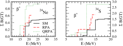
Figure 1: SM (full curve), RPA (dashed), and QRPA(dotted) summed strength for $\beta^{+}$ (left) GT transitions from ²⁴Ne, ³⁴S. The QRPA calculation is from Lau88

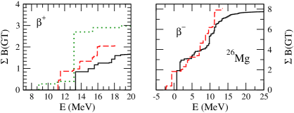
Figure 2: SM (full curve) and RPA (dashed curve) summed strength for $\beta^{+}$ (left) and $\beta^{-}$ (right) GT transitions in ²⁶Mg. For $\beta^{+}$ transitions we also include the QRPA calculation Lau88 (dotted curve)

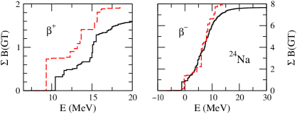
Figure 3: SM (full curve) and RPA (dashed curve) summed strength for $\beta^{+}$ (left) and $\beta^{-}$ (right) GT transitions in ²⁴Na.

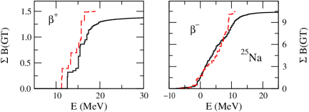
Figure 4: Same as in Fig. 3, but for ²⁵Na.

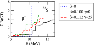
Figure 5: Comparison of the SM (full curve) and pnRPA predictions for the summed strength of GT $\beta^{+}$ transitions in ³²S. The pnRPA was performed on top of a spherical (dotted curve), oblate (dash-dotted), and triaxial (dashed) HF state respectively, emphasizing the importance of a correct treatment of deformation for a correct description of the strength distribution.

IV Conclusions

The main purpose of this paper was to investigate the pnRPA’s reliability for predicting $\beta^{\pm}$ GT transition strengths; the motivation is astrophysical applications, where, aside from binding energies and electomagnetic transitions, a good knowledge of week transitions is essential. Our tool in this investigation was the interacting SM which can provide the exact numerical solution in a restricted space. Although we made our tests for nuclides near the bottom of the valley of stability, presumably our results apply out to the driplines; in fact the major uncertainty will be the shell-model interaction, not the pnRPA.

We show a very good agreement between SM and pnRPA $\beta^{\pm}$ transition distributions in a large number of nuclides in the $sd$ and $pf$ shells, similar to high-lying collective electromagnetic transitions investigated in a previous paper stetcu2003 . Furthermore, we obtain better results than spherical pnQRPA, obtaining better suppression of the total strength. This may seem surprising, as we do not treat rigorously the pairing interaction; on the other hand, we model correctly the deformation and this proves suitable for describing GT transition strengths. (Because of this, we view tests of pnRPA in schematic models without symmetry breaking SMS01 as being inadequate.) It is possible that a deformed pnQRPA approach, with better treatment of pairing, will lead to further improvement. We hope however to extend our program to the deformed pnQRPA in the not-so-distant future. Furthermore, it will be important to consider multi-shell spaces, where at least one set of deformed pnQRPA calculations (not validated by direct shell model calculations, however, due to the enormous size of the model space) suggest a weaker dependence on deformation Sar03 .

- (1) K. Langanke and G. Martinez-Pinedo, Rev. Mod. Phys. 75, 819 (2003).
- (2) Yu. Zdesenko, Rev. Mod. Phys. 74, 663 (2002); F. Boehm and P. Vogel, Physics of Massive Neutrinos, 2nd ed. (Cambridge University Press, Cambridge, England, 1992).
- (3) N. Auerbach, D. C. Zheng, L. Zamick and B. A. Brown, Phys. Lett. B304, 17 (1993).
- (4) B. A. Brown and B. H. Wildenthal, Annu. Rev. Nucl. Part. Sci. 38, 3211 (1991).
- (5) K. Goeke and J. Speth, Ann. Rev. Nucl. Part. Sci. 32, 65 (1982).
- (6) J.U. Nabi and H.V. Klapdor-Kleingrothaus, Acta Phys. Polonica B 30, 825 (1999); Atom. Data Nucl. Data 71, 149 (1999)
- (7) C. Volpe, N. Auerbach, G. Colò, Suzuki, and N. Van Giai, Phys. Rev. C 62, 015501 (2000).
- (8) F. Simkovic, M. Nowak, W. A. Kaminski, A. A. Raduta, and A. Faessler Phys. Rev. C 64, 035501 (2001).
- (9) L. Zhao and B. A. Brown, Phys. Rev. C 47, 2641 (1993).
- (10) J. Engel, P. Vogel, and M. R. Zirnbauer, Phys. Rev. C 37, 731 (1988); J. Engel, S. Pittel, M. Stoitsov, P. Vogel, and J. Dukelsky, Phys. Rev. C 55, 1781 (1997).
- (11) D. J. Rowe, Nuclear Collective Motion (Methuen, London, 1970).
- (12) P. Ring and P. Shuck, The nuclear many-body problem, 1st ed. (Springer-Verlag, New York 1980).
- (13) M. Goldhaber and E. Teller, Phys. Rev. 74, 1046 (1948).
- (14) L.S. Kisslinger and R.A. Sorensen, Rev. Mod. Phys. 35, 853 (1963).
- (15) J. A. Halbleib, Sr., and R. A. Sorensen, Nucl. Phys. A98, 542 (1967); D. Cha, Phys. Rev. C 27, 2269 (1983).
- (16) B. Lauritzen, Nucl. Phys. A489, 237 (1988).
- (17) O. Civitarese, H. Müther, L. .D. Skouras, and A. Faessler, J. Phys. G 17, 1363 (1991).
- (18) N. Auerbach, G. F. Bertsch, B. A. Brown, and L. Zhao, Nucl. Phys. A556, 190 (1993).
- (19) I. Stetcu and C.W. Johnson, Phys. Rev. C 66, 034301 (2002).
- (20) C. W. Johnson and I. Stetcu, Phys. Rev. C 66, 064304 (2002).
- (21) I. Stetcu and C.W. Johnson, Phys. Rev. C 67, 044315 (2003).
- (22) D. Troltenier, J.P. Draayer, and J.G. Hirsch, Nucl. Phys. A 601, 89 (1996).
- (23) D.J. Thouless, Nucl. Phys. 22, 78 (1961).
- (24) E. R. Marshalek and J. Weneser, Ann. Phys. 53, 569 (1969).
- (25) B.H. Wildenthal, Prog. Part. Nucl. Phys. 11, 5 (1984).
- (26) W. A. Richter, M. G. van der Merwe, R. E. Julies and B. A. Brown, Nucl. Phys. A523, 325 (1991).
- (27) R. R. Whitehead,A. Watt, B. J. Cole, and I. Morrison, Adv. Nucl. Phys. 9, 123 (1977).
- (28) R. Nayak, A. Faessler, H. Müther, and A. Watt, Nucl. Phys. A 427, 61 (1984); E. Caurier, A. Poves, and A.P. Zuker, Phys. Lett. B252, 13 (1990); Phys. Rev. Lett 74, 1517 (1995).
- (29) P. Sarriguren et al, Phys. Rev. C. 67, 044313 (2003).
- (30) S. Stoica, I. Mihut, and J. Suhonen, Phys. Rev. C 64, 017303 (2001).