Continuum coupled cluster expansion

Abstract

We review the basics of the coupled-cluster expansion formalism for numerical solutions of the many-body problem, and we outline the principles of an approach directed towards an adequate inclusion of continuum effects in the associated single-energy spectrum. We illustrate our findings by considering the simple case of a single-particle quantum mechanics problem.

I Introduction

One of the major endeavors in modern nuclear physics, is the ongoing quest for an effective nuclear many-body theory, a key element in the attempt to extrapolate existing experimental data to regimes which are not currently accessible in the laboratory. Ideally, one would like to begin with the experimental data available from nucleon-nucleon ($N\!N$) scattering experiments ref:stoks_1990 ; ref:stoks_1993a and determine the underlying $N\!N$ interaction ref:stoks_1994 ; ref:stoks_1993b ; ref:av18 ; ref:rupert_1996 ; ref:rupert_2001 ; ref:rupert_2002 . Subsequent nuclear structure calculations are then necessary to determine a three-nucleon interaction ref:il2 , to account for the remaining differences between theory and experiment.

Direct comparison of theory (calculations) to experimental data is ambiguous if the nuclear many-body problem is not solved accurately. Results of numerical calculations can be used to constrain fundamental aspects of the theory, provided that one has good approximations of the exact result in order to avoid introducing a bias due to the approximations involved. Much progress has been achieved recently by the Green’s Function Monte Carlo (GFMC) ref:carlson_1987 collaboration in obtaining accurate description of nuclear structure properties of light nuclei ($A\leq 10$) ref:PW01 ; ref:PVW02 . Such ab initio calculations, based on realistic interaction models are key for understanding in a quantitative manner the experimental data provided by modern accelerator facilities at Jefferson Laboratory (JLAB) and the future Rare Isotope Accelerator (RIA). We believe that a crucial undertaking in modern physics involves the extension of this work to heavy nuclei.

The limitations of the GFMC method to carry out calculations for arbitrary size nuclei, originate both from the inherent Fermi sign problem associated with a non-relativistic system of nucleons obeying Fermi statistics, and the fact that in the present implementation of the GFMC one carries out explicit summations over the spin-isospin degrees of freedom. As such, the relevant number of degrees of freedom increases as $2^{A}(^{A}_{Z})$, and the size of the spin-isospin vector space quickly becomes prohibitive. A possible way around this technical problem, is offered by the Auxiliary Field Diffusion Monte Carlo (AFDMC) method ref:kevin_1999 , where one attempts to sample the spin-isospin degrees of freedom in addition to the spatial coordinates of the nucleons. This method is currently under development, and encouraging results have been recently reported for neutron matter ref:kevin_2001 .

For nuclei with A$\leq$4, the nonrelativistic Schrödinger equation with realistic nuclear interactions can be solved very precisely: In a recent benchmark ref:kamada02 carried out for a ⁴He-like nucleus using the Argonne v₈’ interaction (central, spin-spin, tensor, spin-orbit and the corresponding spin-exchange counterparts), the binding energy calculated using seven “exact” many-body formalisms agreed within 0.5%. Unfortunately, few many-body formalisms are currently capable to offer accurate numerical solutions of the nuclear many-body problem with realistic interactions, when heavier systems are concerned. For finite nuclei with $A>4$, the no core shell model (NCSM) ref:peter_2000a ; ref:peter_2000b ; ref:peter_2002 and the coupled-cluster expansion (CCE) are the only methods which are able to directly compare results with the GFMC for the same type of hamiltonian. Both methods however have serious limitations related to a slow convergence of the results with the size of the model space. As we are about to describe in this paper, the shortcomings of the CCE are not inherent in nature, and we like to believe that the approach to solving the CCE we propose here, will allow the CCE to provide accurate theoretical output for a medium to large domain of masses, in the framework of realistic nuclear interaction ref:av18 ; ref:uix ; ref:il2 and nuclear currents ref:CS98 . We call this new approach the continuum CCE (c-CCE), because continuum effects are accurately taken in account.

The coupled-cluster expansion (CCE), also called the $\exp({\bf S})$ method, was developed in the early 1960s by Coester and Kümmel ref:C58 ; ref:CK60 . While the method is viewed as exact, approximations are introduced stemming from truncations in the CCE equations, as well as truncations in the model space. Practical approaches for nuclear structure applications have been notoriously difficult to realize. It was not until the 1970s that Zabolitsky and Kümmel ref:Kummel_etal were able to carry out the first detailed calculations for finite nuclei, using a representation of the wave function in coordinate space together with common interactions of the time. The results for the binding energy of nuclei such as ⁴He, ¹⁶O and ⁴⁰Ca, were well above the Coester line and were taken as evidence for the presence of $3N$ and higher-order interactions.

While the CCE was extensively used in other areas in physics and chemistry (see Refs. ref:bishop_review ; ref:navarro_review for additional information), further applications to nuclear structure calculations based on realistic nuclear interactions proved difficult to achieve. In the 1990s we mainly note the attempt of constructing a translationally invariant CCE in coordinate space ref:bishop_1990 ; ref:bishop_1996 ; ref:bishop_1998 , method which might yet offer an attractive alternative for finite nuclei calculations (see Refs. ref:bishop_2000 ; ref:bishop_2002 for information on recent progress on this approach.) To date, however, these attempts are confined to semi-realistic interactions with a V4 structure (scalar plus spin-, isospin-, and space-exchange terms), and the wave functions are not sophisticated enough to provide the realistic account of nuclear forces required in the context of realistic nuclear interactions, such as the Argonne v₁₈ and corresponding three-nucleon forces.

Motivated by the availability of more sophisticated $N\!N$ interactions, and riding the wave of the ongoing expansion in computer power, Heisenberg and Mihaila ref:bm_I ; ref:bm_PRL ; ref:bm_II reexamined the coupled-cluster approach and applied it to the spherical nucleus ¹⁶O, together with a realistic nuclear interaction and currents which were purposely consistent with the work done by the GFMC collaboration: Calculations based on a realistic two-body hamiltonian (Argonne v₁₄ and v₁₈) were reported in Ref. ref:bm_I , while effects of a phenomenological three-body interaction (Urbana IX) were reported in Ref. ref:bm_II . An extension of the later application, involved the microscopic calculation of the charge form factor in ¹⁶O. Results were presented in Ref. ref:bm_PRL , and showed good agreement with the available experimental data ref:sick_o16 when both three-body forces and meson-exchange currents were taken into account.

In its present implementation the CCE equations are solved for the special case of spin-isospin shell-saturated nuclei, such as ⁴He, ^12,14C, ^14,16O. In order to depart from the closed-shell case one resorts to an equation of motion approach, using the ground-state of the closed-shell nucleus as a new vacuum. As such one can describe the properties of hole-state nuclei such as ¹³C and ¹⁵N, and preliminary results are promising. However, such an approach will inevitably compound the effect of new and old approximations. Also, the present approach has limitations due to the intrinsic cutoffs one has to impose when defining the model configuration space. The single particle states are expanded in a harmonic oscillator basis, and satisfy the same type of boundary conditions for both hole and particle states. In effect we discretize the continuum part of the self-consistent one-body mean-field hamiltonian used to define the single-energy spectrum. This results in the necessity of a large $50\hbar\Omega$ configuration space and subsequent significant storage problems and lengthy execution time.

One would like to obtain exact solutions for the 2-, 3- and 4-body systems via CCE. Since contributions due to $n>A$ particle-hole configurations are always cancelled exactly, the above few-body systems will provide scenarios when the truncation of the CCE hierarchy for $A=2$, $3$ and $4$, respectively, becomes exact, and we will be able to reliably ascertain the numerical accuracy by direct comparison with similar results obtained via other exact methods. Moreover, by solving the two- and three-body problem, we will effectively eliminate our present reliance on the closed-shell hypothesis, and allow for direct calculations of nuclei inside the shell via CCE. Given our past experience regarding the ground state calculation of spin-isospin shell-saturated nuclei in configuration space, we can expect that a four-cluster truncation of the CCE equations will allow an accurate description of arbitrary nuclei beyond $A=16$.

From a numerical standpoint, we must always remember that we have to solve a finite physical system, using finite computational resources, in a finite amount of time. We submit that the resolution of the many-body problem is linked to the successful design of a numerical algorithm that allows for an efficient implementation on a massively multiprocessor machines. In order to preserve the scalability of a numerical algorithm on a multiprocessor machine, we propose to address the problem of finding the energy spectrum of the hamiltonian by strictly following the two commandments:

1. Thou shalt not solve matrix eigenvalue equations.

2. Thou shalt not perform explicit matrix inversions.

In order to solve this conundrum, we must pursue those iterative numerical schemes which are most likely approachable using Monte Carlo techniques. It is our contention that the basic expertise for solving the nuclear many-body problem is available at this time: The GFMC is the only many-body method available today that obeys the above constraints. However, in its present formulation, the GFMC carries out explicit summations over all possible spin-isospin combinations, and this leads to a $2^{A}(^{A}_{Z})$ increase for the number of the relevant degrees of freedom. We propose to investigate the possibility of solving a comparatively small ($n\leq 4$)-cluster truncation of the CCE hierarchy of equations using Monte Carlo techniques. Assuming the CCE truly exhibits a $1/A$-type convergence, then it is reasonable to expect that approximations based on the CCE will accurately describe nuclear structure with realistic nuclear interactions and currents, around and beyond ¹⁶O. The CCE equations will still involve explicit spin-isospin summations, but these will entail only minimal complications because the small size of the cluster will drastically simplify the problem.

To summarize, our long-range interest is two-fold: firstly, we want to develop a continuum version of the CCE in an attempt to efficiently describe physics at large distances; secondly, we are interested in finding an efficient numerical procedure to solve the CCE equations. We find it useful to begin our investigations with the simplest dimensional realization of the many-body problem: the one-body case, $A=1$. The mere simplicity of the problem will allow for an exhaustive, detailed study of the CCE equations.

II Single-energy spectrum

Consider the Hilbert space of states associated with the one-body hamiltonian

$${\mathbf{H}}_{0}={\mathbf{T}}+{\mathbf{V}_{0}}\>,$$ (1)

and a basis set in this Hilbert space. In general, this basis features both a discrete and a continuum part, such that any state in the Hilbert space can be expanded as

$$|\psi\rangle=\sum_{n}a_{n}|\phi_{n}\rangle+\int\frac{\mathrm{d}^{3}p}{(2\pi)^{3}}\ b_{\vec{p}}|\phi_{\vec{p}}\rangle\>.$$ (2)

That is to say that the basis states in the spectrum satisfy the orthonormality relations

$$\langle\phi_{n}|\phi_{m}\rangle =\delta_{nm}\>,$$ (3a)

$$\langle\phi_{\vec{p}}|\phi_{\vec{p^{\prime}}}\rangle =(2\pi)^{3}\,\delta(\vec{p}-\vec{p^{\prime}})=\delta_{\vec{p}\vec{p^{\prime}}}\>,$$ (3b)

$$\langle\phi_{n}|\phi_{\vec{p}}\rangle =0\>,$$ (3c)

and the basis set is complete

$$\sum_{n}|\phi_{n}\rangle\langle\phi_{n}|+\int\frac{\mathrm{d}^{3}p}{(2\pi)^{3}}\ |\phi_{\vec{p}}\rangle\langle\phi_{\vec{p}}|=\delta(\vec{r}-\vec{r^{\prime}})\>.$$ (4)

The above basis can be the same as, but is not restricted to, the set of eigenvectors corresponding to the single-energy spectrum defined by the solutions of the Schrödinger equation

$${\mathbf{H}}_{0}\ |\phi\rangle\ =\ \varepsilon\ |\phi\rangle\>.$$ (5)

We propose to start with a known set of discrete single particle wave functions $\{\phi_{n}\}$ in the above Hilbert space, which satisfy Eq. (3a), and subsequently construct a set $\{\phi_{\vec{p}}\}$, which obeys the remaining orthonormality conditions, Eqs. (3b,3c), the closure relation (4), and satisfies a predetermined boundary condition (i.e. bound state or scattering state).

This can be done as follows: In order to satisfy the orthogonality conditions between the appropriate continuum single-particle wave functions, we start with a complete set of continuum wave functions

$$|\bar{\chi}_{\vec{p}}\rangle=|\chi_{\vec{p}}\rangle-\sum_{n}|\phi_{n}\rangle\langle\phi_{n}|\chi_{\vec{p}}\rangle\>.$$ (6)

For instance, if the continuum wave function $\chi_{\vec{p}}(\vec{r})$ is just a plane wave, $\chi_{\vec{p}}(\vec{r})=e^{\mathrm{i}\,\vec{p}\cdot\vec{r}}$, then $\langle\phi_{n}|\chi_{\vec{p}}\rangle=\tilde{\phi}_{n}(\vec{p})$ denote the Fourier transform of the wave function $\phi_{n}(\vec{r})$. The set of continuum wave functions $\{\bar{\chi}_{\vec{p}}\}$ are orthogonal to the discrete spectrum of the hamiltonian, i.e. $\langle\phi_{n}|\bar{\chi}_{\vec{p}}\rangle=0$, and satisfy the completeness relation

$$\sum_{n}|\phi_{n}\rangle\langle\phi_{n}|+\int\frac{\mathrm{d}^{3}p}{(2\pi)^{3}}\ |\bar{\chi}_{\vec{p}}\rangle\langle\bar{\chi}_{\vec{p}}|=\delta(\vec{r}-\vec{r^{\prime}})\>.$$ (7)

These wave functions however are not orthogonal to each other

$$\langle\bar{\chi}_{\vec{p}}|\bar{\chi}_{\vec{p^{\prime}}}\rangle=\delta_{\vec{p}\vec{p^{\prime}}}-\sum_{n}\tilde{\phi}_{n}^{*}(\vec{p})\ \tilde{\phi}_{n}(\vec{p^{\prime}})\>.$$ (8)

Without loss of generality we can orthonormalize this set $\{\bar{\chi}_{\vec{p}}\}$ to obtain the desired set of continuum wave functions, $\{\phi_{\vec{p}}\}$. Note that there is no inconsistency here, since $\bar{\chi}_{\vec{p}}(\vec{r})$ is not simply a linear superposition of plane waves, but we can define $\phi_{\vec{p}}(\vec{r})$ as a linear combination of $\bar{\chi}_{\vec{p}}(\vec{r})$ in order to perform the orthonormalization. In practice, the fact that the definition of $\bar{\chi}_{\vec{p}}(\vec{r})$ involves the Fourier transform of $\phi_{n}(\vec{r})$, establishes the appropriate grid representation of the single-particle wave functions. The set $\{\phi_{\vec{p}}\}$ is obtained by orthonormalization of the set $\{\bar{\chi}_{\vec{p}}\}$ at these grid points. This concludes our construction.

The fact we actually have to normalize the continuum basis states on a grid, may be a serious drawback. After all we started this process with the idea in mind that a formal discretization of the continuum prevents us from obtaining rigorous numerical convergence with modest computational resources. It is therefore unfortunate that an actual discretization appears to be necessary at this point. However, we claim that already at this point we are better off in this formalism since all basis states, and most importantly the continuum basis states, have the correct boundary conditions built in. Moreover, we will see that the above construction is not binding us into a certain course of action. We will argue later, that we can in fact circumvent these apparent difficulties, and return to a representation formulated entirely in coordinate space where the explicit knowledge of the continuum states is not mandatory.

III Second quantization

We proceed now by outlining the second quantization language we will subsequently use. We start by introducing the field operators $\mathbf{\hat{\psi}}(\vec{r})$ and $\mathbf{\hat{\psi}}^{\dagger}(\vec{r})$, as linear combinations of creation and destruction operators ${\mathbf{c}}_{\alpha},{\mathbf{c}}^{\dagger}_{\alpha}$, respectively:

$$\mathbf{\hat{\psi}}(\vec{r}) =\sum_{\alpha}\phi_{\alpha}(\vec{r})\ {\mathbf{c}}_{\alpha}$$ (9)

$$\equiv\sum_{n}\ \phi_{n}(\vec{r})\ {\mathbf{b}}^{\dagger}_{n}\ +\ \int\frac{\mathrm{d}^{3}p}{(2\pi)^{3}}\ \phi_{\vec{p}}(\vec{r})\ {\mathbf{a}}_{\vec{p}}\>,$$

where the single-particle wave functions $\phi(\vec{r})\equiv\{\phi_{n}(\vec{r}),\phi_{\vec{p}}(\vec{r})\}$, form a complete basis, and satisfy the orthonormality properties, as explained in the previous section. The inverse transformations are

$${\mathbf{b}}^{\dagger}_{n} =\int\mathrm{d}^{3}r\ \phi_{n}^{*}(\vec{r})\,\mathbf{\hat{\psi}}(\vec{r})\>,$$ (10)

$${\mathbf{a}}_{\vec{p}} =\int\mathrm{d}^{3}r\ \phi_{\vec{p}}^{*}(\vec{r})\,\mathbf{\hat{\psi}}(\vec{r})\>.$$ (11)

In other words, ${\mathbf{b}}^{\dagger}_{n}$ removes a nucleon from the hole orbit $\phi_{n}(\vec{r})$, while ${\mathbf{a}}_{\vec{p}}$ removes a nucleon from a particle orbit $\phi_{\vec{p}}(\vec{r})$. With these definitions, we can write

$${\mathbf{c}}^{\dagger}=\left\{\begin{matrix}{\mathbf{a}}^{\dagger}_{\vec{p}}\>,&\mathrm{if}\ \varepsilon_{p}\geq\varepsilon_{F}\>,\\ {\mathbf{b}}_{n}\>,&\mathrm{if}\ \varepsilon_{n}<\varepsilon_{F}\>,\end{matrix}\right.$$ (12)

and

$${\mathbf{c}}=\left\{\begin{matrix}{\mathbf{a}}_{\vec{p}}\>,&\mathrm{if}\ \varepsilon_{p}\geq\varepsilon_{F}\>,\\ {\mathbf{b}}^{\dagger}_{n}\>,&\mathrm{if}\ \varepsilon_{n}<\varepsilon_{F}\>.\end{matrix}\right.$$ (13)

Here, $\varepsilon_{F}$ denotes the Fermi energy. Note that in the region between the Fermi energy and the separation energy $(\varepsilon_{p}=0)$, the “continuum” spectrum, $|\phi_{\vec{p}}\rangle$, is actually discrete, and the integral has to be interpreted as a sum.

Since we are interested in many-body systems obeying fermi statistics, we ask the field operators to obey the anti-commutation relations

$$\Bigl{\{}\mathbf{\hat{\psi}}^{\dagger}(\vec{r}),\,\mathbf{\hat{\psi}}(\vec{r^{\prime}})\Bigr{\}}=\delta(\vec{r}-\vec{r^{\prime}})\>.$$ (14)

Spin and isospin indices are implied. In turn, the creation and annihilation operators obey the canonical relations:

$$\{{\mathbf{c}}^{\dagger}_{n},{\mathbf{c}}_{m}\}=\delta_{nm}\>,\qquad\{{\mathbf{c}}^{\dagger}_{\vec{p}},{\mathbf{c}}_{\vec{p^{\prime}}}\}=\delta_{\vec{p}\vec{p^{\prime}}}\>,$$

$$\{{\mathbf{c}}_{n},{\mathbf{c}}_{m}\}=\{{\mathbf{c}}^{\dagger}_{n},{\mathbf{c}}^{\dagger}_{m}\}=\{{\mathbf{c}}_{\vec{p}},{\mathbf{c}}_{\vec{p^{\prime}}}\}=\{{\mathbf{c}}^{\dagger}_{\vec{p}},{\mathbf{c}}^{\dagger}_{\vec{p^{\prime}}}\}=0\>,$$

$$\{{\mathbf{c}}_{n},{\mathbf{c}}_{\vec{p}}\}=\{{\mathbf{c}}^{\dagger}_{n},{\mathbf{c}}^{\dagger}_{\vec{p}}\}=\{{\mathbf{c}}^{\dagger}_{n},{\mathbf{c}}_{\vec{p}}\}=\{{\mathbf{c}}_{n},{\mathbf{c}}^{\dagger}_{\vec{p}}\}=0\>,$$

or

$$\{{\mathbf{b}}^{\dagger}_{n},{\mathbf{b}}_{m}\}=\delta_{nm}\>,\qquad\{{\mathbf{a}}^{\dagger}_{\vec{p}},{\mathbf{a}}_{\vec{p}^{\prime}}\}=\delta_{\vec{p}\vec{p^{\prime}}}\>,$$

$$\{{\mathbf{b}}_{n},{\mathbf{b}}_{m}\}=\{{\mathbf{b}}^{\dagger}_{n},{\mathbf{b}}^{\dagger}_{m}\}=\{{\mathbf{a}}_{\vec{p}},{\mathbf{a}}_{\vec{p}^{\prime}}\}=\{{\mathbf{a}}^{\dagger}_{\vec{p}},{\mathbf{a}}^{\dagger}_{\vec{p}^{\prime}}\}=0\>,$$

$$\{{\mathbf{b}}_{n},{\mathbf{a}}_{\vec{p}}\}=\{{\mathbf{b}}^{\dagger}_{n},{\mathbf{a}}^{\dagger}_{\vec{p}}\}=\{{\mathbf{b}}^{\dagger}_{n},{\mathbf{a}}_{\vec{p}}\}=\{{\mathbf{b}}_{n},{\mathbf{a}}^{\dagger}_{\vec{p}}\}=0\>.$$

More definitions are in order: We introduce the bare vacuum, $|0\rangle$, such that

$$\mathbf{\hat{\psi}}(\vec{r})\,|0\rangle=0\>,$$ (17)

or

$${\mathbf{a}}_{\vec{p}}\,|0\rangle=0\>,\qquad{\mathbf{b}}^{\dagger}_{n}\,|0\rangle=0\>.$$ (18)

In turn, the physical vacuum, $|\Phi\rangle$, which will play the role of the reference state for $\exp({\mathbf{S}})$, is defined as the exhaustive collection of minimal configurations of a given symmetry, obtainable from the bare vacuum:

$${\mathbf{a}}_{\vec{p}}\,|\Phi\rangle=0\>,\qquad{\mathbf{b}}_{n}\,|\Phi\rangle=0\>.$$ (19)

We have

$${\mathbf{c}}^{\dagger}_{\vec{p}}|\Phi\rangle={\mathbf{a}}^{\dagger}_{\vec{p}}|\Phi\rangle\>,\qquad{\mathbf{c}}_{n}|\Phi\rangle={\mathbf{b}}^{\dagger}_{n}|\Phi\rangle\>.$$ (20)

Finally, the second quantization representation of the one-body hamiltonian operator is given by

$${\mathbf{H}}\ =\ \sum_{\alpha\beta}{\mathbf{c}}^{\dagger}_{\alpha}\,\langle\phi_{\alpha}|{\mathbf{H}}|\phi_{\beta}\rangle\,{\mathbf{c}}_{\beta}\>.$$ (21)

By the same token, we will represent for instance, the 1$p$1$h$ cluster-correlation operator, as

$${\mathbf{S}}_{1}\ =\ \sum_{n}\ \int\frac{\mathrm{d}^{3}p}{(2\pi)^{3}}\ {\mathbf{a}}^{\dagger}_{\vec{p}}\,S_{\vec{p}n}\,{\mathbf{b}}^{\dagger}_{n}\>.$$ (22)

IV CCE equations

In a traditional shell-model approach, one calculates the matrix elements of the hamiltonian

$$\langle\Psi_{1}|{\mathbf{H}}|\Psi_{2}\rangle = \sum_{mn}a_{n}^{(1)*}a_{m}^{(2)}\langle\phi_{n}|{\mathbf{H}}|\phi_{m}\rangle$$

$$+\sum_{m}\int\frac{\mathrm{d}^{3}p}{(2\pi)^{3}}\ b_{\vec{p}}^{*}a_{m}^{(2)}\langle\phi_{\vec{p}}|{\mathbf{H}}|\phi_{m}\rangle$$

$$+\sum_{n}\int\frac{\mathrm{d}^{3}p^{\prime}}{(2\pi)^{3}}\ a_{n}^{(1)*}b_{\vec{p^{\prime}}}\langle\phi_{n}|{\mathbf{H}}|\phi_{\vec{p^{\prime}}}\rangle$$

$$+\int\frac{\mathrm{d}^{3}p}{(2\pi)^{3}}\ \int\frac{\mathrm{d}^{3}p^{\prime}}{(2\pi)^{3}}\ b_{\vec{p}}^{*}b_{\vec{p^{\prime}}}\langle\phi_{\vec{p}}|{\mathbf{H}}|\phi_{\vec{p^{\prime}}}\rangle\>.$$

Then, for an arbitrary eigenstate of the hamiltonian, $|\Psi\rangle$, we write the Schrödinger equation

$${\mathbf{H}}\ \sum_{\alpha}|\Psi_{\alpha}\rangle\langle\Psi_{\alpha}|\Psi\rangle=E\ \sum_{\alpha}|\Psi_{\alpha}\rangle\langle\Psi_{\alpha}|\Psi\rangle\>,$$ (24)

which leads to the usual eigenvalue problem

$$\sum_{\beta}\Bigl{(}\langle\Psi_{\alpha}|{\mathbf{H}}|\Psi_{\beta}\rangle-E_{\alpha}\delta_{\alpha\beta}\Bigr{)}\,\langle\Psi_{\beta}|\Psi\rangle\ =\ 0\>.$$ (25)

We make the convention that Greek indices run over both the discrete and continuum spectra, i.e. the sum $\sum_{\alpha}$ is in fact a sum over the discrete, and an integral over the continuum. When solving the above eigenvalue, one is usually forced to discretize the continuum: one uses a discrete basis, which results into a finite matrix, which can then be diagonalized using regular linear algebra numerical packages.

We would like to avoid this approach. Therefore, rather than calculating the “entire” spectrum of the hamiltonian at the same time, we will attempt to calculate the spectrum of the hamiltonian one state at a time, similar to the GFMC approach. In the same spirit, we will attempt to calculate observables without explicit knowledge of the actual wave functions: wave functions are not observables, and we will concentrate on developing a formalism allowing direct calculation of the expectation values of operators.

In the CCE formalisms, one first introduces an ansatz for the eigenstate $|\Psi\rangle$ of the hamiltonian

$$|\Psi\rangle\ =\ e^{{\mathbf{S}}}\ |\Phi\rangle\>,$$ (26)

where $|\Phi\rangle$ is the physical vacuum or reference state. The ansatz for $|\Psi\rangle$ satisfies the normalization condition

$$\langle\Psi|\Phi\rangle=1\>.$$ (27)

Here ${\mathbf{S}}$ denotes the many-body cluster-correlation operator:

$${\mathbf{S}}\ =\ \sum_{n=1}^{A}\ S_{n}\,{\mathbf{O}}^{\dagger}_{n}\>,$$ (28)

where ${\mathbf{O}}^{\dagger}_{n}$ denotes an n$p$n$h$-configuration creation operator. Mathematically speaking, the interpretation of a n$p$n$h$ configuration is that an element of a basis set spanning the many-body Hilbert space. For a given n$p$n$h$ configuration, the correlation function for $n$-nucleons, or the n$p$n$h$ correlation coefficients $S_{n}$, is simply the associated expansion coefficient.

We emphasize that the physical vacuum, $|\Phi\rangle$, is defined as the minimal set of configurations obtained from the bare vacuum, which obey a certain set of symmetries and boundary conditions. Appropriate choices can be made for $|\Phi\rangle$ which will allow us to independently construct both the ground state and excited state spectrum of the hamiltonian, without changing the single-energy spectrum. The cluster-correlation operator is a rank-zero tensor operator and will leave unchanged both the symmetry and boundary conditions of $|\Phi\rangle$. Therefore, the information regarding a particular set of quantum numbers is contained in the physical vacuum $|\Phi\rangle$; properties such as orthogonality of the various eigenstates will be satisfied by construction. In so doing, we depart from prior attempts to obtain the excited state spectrum of the hamiltonian by means of an equation of motion approach which relies on a prior calculation of the ground state.

With these definitions, the Schrödinger equation for the eigenstate $|\Psi\rangle$ of the hamiltonian corresponding to a chosen symmetry,

$${\mathbf{H}}|\Psi\rangle=E|\Psi\rangle\>,$$ (29)

becomes

$$e^{-{\mathbf{S}}}{\mathbf{H}}e^{{\mathbf{S}}}\ |\Phi\rangle\ =\ E\ |\Phi\rangle\>,$$ (30)

or, in normal ordered form,

$$\left(e^{-{\mathbf{S}}}{\mathbf{H}}e^{{\mathbf{S}}}\right)_{c}\ |\Phi\rangle\ =\ E\ |\Phi\rangle\>,$$ (31)

where the subscript $c$ indicates the pure creation part of a normal ordered operator. In principle, the resulting system of integral equations must be solved for the n$p$n$h$ correlation amplitudes $S_{n}$ and the energy $E$. It is desirable, and in the spirit of the approach we initiate in this paper, to design a way of calculating $E$ without explicitly calculating (and storing!) $S_{n}$.

V Observables

Consider the expectation value of an arbitrary operator ${\mathcal{O}}$

$$\bar{o}\ =\ \frac{\langle\Psi|{\mathcal{O}}|\Psi\rangle}{\langle\Psi|\Psi\rangle}\>.$$ (32)

We perform the following transformations

$$\bar{o}\ =\ \frac{\langle\Phi|e^{{\mathbf{S}}^{\dagger}}{\mathcal{O}}e^{{\mathbf{S}}}|\Phi\rangle}{\langle\Psi|\Psi\rangle}$$

$$\ =\ \frac{\langle\Phi|e^{{\mathbf{S}}^{\dagger}}e^{{\mathbf{S}}}\ e^{-{\mathbf{S}}}{\mathcal{O}}e^{{\mathbf{S}}}|\Phi\rangle}{\langle\Psi|\Psi\rangle}\>.$$

We can insert a complete set of n$p$n$h$ configurations, and obtain

$$\bar{o}\ =\ \sum_{n}\ \frac{\langle\Phi|e^{{\mathbf{S}}^{\dagger}}e^{{\mathbf{S}}}\ {\mathbf{O}}^{\dagger}_{n}|\Phi\rangle}{\langle\Psi|\Psi\rangle}\ \langle\Phi|{\mathbf{O}}_{n}\ e^{-{\mathbf{S}}}{\mathcal{O}}e^{{\mathbf{S}}}|\Phi\rangle$$

$$\ =\ \sum_{n}\ \frac{\langle\Psi|{\mathbf{O}}^{\dagger}_{n}|\Psi\rangle}{\langle\Psi|\Psi\rangle}\ \langle\Phi|{\mathbf{O}}_{n}\ e^{-{\mathbf{S}}}{\mathcal{O}}e^{{\mathbf{S}}}|\Phi\rangle\>,$$

where in the last step we have used the fact that ${\mathbf{O}}^{\dagger}_{n}$ and ${\mathbf{S}}$ commute. We introduce a new cluster-correlation operator, $\tilde{\mathbf{S}}$, by its many-body decomposition, as

$$\tilde{\mathbf{S}}\ =\ \sum_{n}\ \frac{\langle\Psi|{\mathbf{O}}^{\dagger}_{n}|\Psi\rangle}{\langle\Psi|\Psi\rangle}\ {\mathbf{O}}_{n}\ =\ \sum_{n}\ \tilde{S}_{n}\,{\mathbf{O}}_{n}\>.$$ (33)

Note that

$$\tilde{S}_{n}\ =\ \frac{\langle\Psi|{\mathbf{O}}^{\dagger}_{n}|\Psi\rangle}{\langle\Psi|\Psi\rangle}\ =\ \frac{\langle\Psi|{\mathbf{O}}_{n}|\Psi\rangle}{\langle\Psi|\Psi\rangle}\ \>,$$ (34)

and therefore the $\tilde{S}_{n}$ amplitudes are real. With this definition, we can calculate the expectation value of the operator ${\mathcal{O}}$ as

$$\bar{o}\ =\ \langle\Phi|\tilde{\mathbf{S}}\ e^{-{\mathbf{S}}}{\mathcal{O}}e^{{\mathbf{S}}}|\Phi\rangle\ =\ \langle\Phi|e^{{\mathbf{S}}^{\dagger}}{\mathcal{O}}e^{-{\mathbf{S}}^{\dagger}}\ \tilde{\mathbf{S}}^{\dagger}|\Phi\rangle\>.$$ (35)

Based on the (second) definition of the n$p$n$h$ amplitudes

$$\tilde{S}_{n}\ =\ \langle\Phi|\tilde{\mathbf{S}}\ e^{-{\mathbf{S}}}{\mathbf{O}}_{n}e^{{\mathbf{S}}}|\Phi\rangle\>,$$ (36)

we can determine $\tilde{S}_{n}$ via an iterative procedure.

Note that the correlated ground state $|\Psi\rangle$ is not a translational-invariant wave function. Therefore, in practice one must correct for the effects of the center-of-mass (CM) motion. In our previous studies, a many-body expansion has been devised to evaluate the corrections required by the calculation of observables in the CM frame ref:bmCM . The accuracy of the proposed procedure was tied to the success of a good separation of the CM and relative coordinates degrees of freedom in the CCE solution. This hypothesis was tested ref:bm_II by adding to the Hamiltonian a purely CM piece, multiplied by a strength parameter, and making sure that the binding energy is independent of this parameter.

We review this issue now on fundamental grounds: In order to produce translational-invariant many-body wave functions, one must seek a simultaneous eigenvalue of both the hamiltonian and the total momentum of the system:

$${\mathbf{H}}\ |\Psi\rangle\ =\ E\ |\Psi\rangle\>,$$ (37)

$${\mathbf{P}}\ |\Psi\rangle\ =\ \vec{P}\ |\Psi\rangle\>,$$ (38)

or

$$e^{-{\mathbf{S}}}{\mathbf{H}}e^{{\mathbf{S}}}\ |\Phi\rangle\ =\ E\ |\Phi\rangle\>,$$ (39)

$$e^{-{\mathbf{S}}}{\mathbf{P}}e^{{\mathbf{S}}}\ |\Phi\rangle\ =\ \vec{P}\ |\Phi\rangle\>.$$ (40)

A closer inspection of the above set of equations shows that this not an over-determined system of equations: By definition, the hamiltonian is the internal hamiltonian of the many-body system, where the CM kinetic energy has been removed. The following commutators are identically zero:

$$[{\mathbf{H}},\,{\mathbf{P}}]\ =\ \bigl{[}e^{-{\mathbf{S}}}{\mathbf{H}}e^{{\mathbf{S}}},\,e^{-{\mathbf{S}}}{\mathbf{P}}e^{{\mathbf{S}}}\bigr{]}\ =\ 0\>.$$ (41)

One can replace Eq. (40) with a linear combination of Eqs. (39) and (40) :

$$e^{-{\mathbf{S}}}[{\mathbf{H}},\,{\mathbf{P}}]e^{{\mathbf{S}}}\ |\Phi\rangle\ =\ 0\>.$$ (42)

Since the hamiltonian and the total momentum commute, it follows that this equation is always satisfied by a solution of Eq. (39). Therefore, the dressed hamiltonian, $e^{-{\mathbf{S}}}{\mathbf{H}}e^{{\mathbf{S}}}$, does not modify the CM degrees of freedom content of the physical vacuum, $|\Phi\rangle$.

In practice one has to truncate the CCE hierarchy of equations, and an inadequate truncation may render the above discussion inconsequential. However, the above statements remain valid for a truncated version of the CCE, provided that a truncated cluster-correlation operator ${\mathbf{S}}^{(N)}$ can be defined, and ${\mathbf{S}}^{(N)}$ satisfies the identities

$$e^{-{\mathbf{S}}^{(N)}}\,e^{{\mathbf{S}}^{(N)}}\ =\ 1\>,$$ (43)

and

$$e^{-{\mathbf{S}}^{(N)}}{\mathcal{O}}\ e^{{\mathbf{S}}^{(N)}}\ =\ {\mathcal{O}}+[{\mathcal{O}},{\mathbf{S}}^{(N)}]$$ (44)

$$+\frac{1}{2!}\bigl{[}[{\mathcal{O}},{\mathbf{S}}^{(N)}],{\mathbf{S}}^{(N)}\bigr{]}+\cdots\>.$$

An acceptable truncation of the CCE hierarchy is generated by the prescription

$$S_{n}=0,\ n>N\>.$$ (45)

The physical vacuum plays indeed a key role in the CCE formalism: When done correctly, and even if $|\Phi\rangle$ breaks certain symmetries of the desired solution, the CCE will leave the center-of-mass part of the physical vacuum unchanged. Therefore, one can perform corrections at the level of the physical vacuum, and the further inclusion of the n$p$n$h$ correlations will leave these corrections unchanged. This is an important observation, since we have the physical vacuum in closed form, and we would rather not explicitly calculate the n$p$n$h$ correlations. If $|\Phi\rangle$ can be written as the product of a CM wave function and a wave function of the system with respect to the center-of-mass, then one can carry out the CM corrections via a simple correction factor, just like in the shell model with harmonic oscillator wave functions.

VI $A=1$ : Single-particle quantum mechanics

So far, our discussion has been quite general. We will particularize now to the simplest possible case, namely the case of a single-particle quantum mechanics problem. The CCE is a many-body formalism, but the procedure is quite general, and we can apply it to the $A=1$ case. In this context, we will continue using the many-body language, and refer to “configurations” and “correlations”, but solely because this is an intrinsic part of the CCE formalism.

In the one-body case, the cluster-correlation operator is particularly simple

$${\mathbf{S}}\ =\ {\mathbf{S}}_{1}\>.$$ (46)

Since the cluster-correlation operator contains only 1$p$1$h$ correlations Eq. (26) can be written as

$$|\Psi\rangle\ =\ e^{{\mathbf{S}}}\ |\Phi\rangle\ =\ (\mathbf{1}+{\mathbf{S}})\ |\Phi\rangle\>,$$ (47)

where no matter what symmetry we are interested in, there is only one possible configuration in $|\Phi\rangle$. We introduce the physical vacuum for the one-body case, as

$$|\Phi\rangle\ =\ |\phi_{h}\rangle\>.$$ (48)

For simplicity, we will consider that $|\phi_{h}\rangle$ is the only state in the discrete spectrum satisfying the required symmetry. An extension to the case when we have more than one discrete state in the spectrum is straightforward and the relevant equations will be relegated to Appendix B.

In order to derive the corresponding CCE equations we use the identity (see also Appendix A)

$$e^{-{\mathbf{S}}}{\mathbf{H}}e^{{\mathbf{S}}} = {\mathbf{H}}+[{\mathbf{H}},{\mathbf{S}}_{1}]+\frac{1}{2!}\bigl{[}[{\mathbf{H}},{\mathbf{S}}_{1}],{\mathbf{S}}_{1}\bigr{]}\>.$$ (49)

Then, Eq. (31) is equivalent to the following set of equations

$$E = \left({\mathbf{H}}\right)_{0}+\left([{\mathbf{H}},{\mathbf{S}}_{1}]\right)_{0}\>,$$ (50)

$$0 = \left({\mathbf{H}}\right)_{1}+\left([{\mathbf{H}},{\mathbf{S}}_{1}]\right)_{1}+\frac{1}{2!}\left(\bigl{[}[{\mathbf{H}},{\mathbf{S}}_{1}],{\mathbf{S}}_{1}\bigr{]}\right)_{1}\>.$$ (51)

These equations are solved for the energy $E$ corresponding to $|\Psi\rangle$, and the correlations $S_{1}$.

Using Eqs. (46) and (47) we can write the solution of the Schrödinger equation as

$$|\Psi\rangle\ =\ |\phi_{n}\rangle+\int\frac{\mathrm{d}^{3}p}{(2\pi)^{3}}\ S_{\vec{p}h}|\phi_{\vec{p}}\rangle\>.$$ (52)

We note that for the one-body problem, it is particularly simple to find an interpretation or an independent check for the CCE equations. Based on Eqs. (47) and (29), we can readily derive

$$E\ =\ \langle\phi_{h}|{\mathbf{H}}|\Psi\rangle\>,$$ (53)

$$E\,S_{\vec{p}h}\ =\ \langle\phi_{p}|{\mathbf{H}}|\Psi\rangle\>.$$ (54)

Using the commutators listed in Appendix A, the CCE equations we need to solve become

$$E \ =\ \langle\phi_{h}|{\mathbf{H}}|\phi_{h}\rangle+\int\frac{\mathrm{d}^{3}p}{(2\pi)^{3}}\ \langle\phi_{h}|{\mathbf{H}}|\phi_{\vec{p}}\rangle\,S_{\vec{p}h}\>,$$ (55)

$$0 =\langle\phi_{\vec{p}}|{\mathbf{H}}|\phi_{h}\rangle$$

$$+\int\frac{\mathrm{d}^{3}p_{1}}{(2\pi)^{3}}\ \langle\phi_{\vec{p}}|{\mathbf{H}}|\phi_{\vec{p}_{1}}\rangle\,S_{\vec{p_{1}}h}-S_{\vec{p}h}\,\langle\phi_{h}|{\mathbf{H}}|\phi_{h}\rangle$$

$$-\int\frac{\mathrm{d}^{3}p_{1}}{(2\pi)^{3}}\ S_{\vec{p}h}\,\langle\phi_{h}|{\mathbf{H}}|\phi_{\vec{p}_{1}}\rangle\,S_{\vec{p_{1}}h}\>.$$ (56)

By inspection, the last equation gives

$$E\,S_{\vec{p}h}= \langle\phi_{\vec{p}}|{\mathbf{H}}|\phi_{h}\rangle+\int\frac{\mathrm{d}^{3}p_{1}}{(2\pi)^{3}}\ \langle\phi_{\vec{p}}|{\mathbf{H}}|\phi_{\vec{p}_{1}}\rangle\,S_{\vec{p_{1}}h}\>.$$ (57)

Equations (55) and (57) involve explicit integrals over correlations in momentum space, and we will refer to this set of equations as the $P$-set. These equations are entirely consistent with Eqs. (53) and (54) above.

We note for completeness, that by formally introducing the notations

$$v_{\vec{p}}\ =\ \langle\phi_{\vec{p}}|{\mathbf{H}}|\phi_{h}\rangle\>,$$ (58)

$$v_{\vec{p}}^{T}\ =\ \langle\phi_{h}|{\mathbf{H}}|\phi_{\vec{p}}\rangle\>,$$ (59)

$$A_{\vec{p}_{1}\vec{p}_{2}}\ =\ E\,\delta_{\vec{p}_{1}\vec{p}_{2}}-\langle\phi_{\vec{p}_{1}}|{\mathbf{H}}|\phi_{\vec{p}_{2}}\rangle\>,$$ (60)

the solution of $P$-set of equations can be formally obtained as

$$S_{1}\ =\ [A]^{-1}\,v\>,$$ (61)

$$E\ =\ \langle\phi_{h}|{\mathbf{H}}|\phi_{h}\rangle\ +\ v^{T}\,\cdot\,[A]^{-1}\,v\>.$$ (62)

This implies, of course, that in order to get the energy, one has again to discretize the continuum, and the solution is obtained by inverting a matrix. The procedure is iterated until convergence is achieved. We do not propose using this approach.

The above momentum space integrals can be avoided in favor of a coordinate representation: We begin by introducing the hole-function

$$\chi_{h}(\vec{r})\ =\ \int\frac{\mathrm{d}^{3}p}{(2\pi)^{3}}\ \phi_{\vec{p}}(\vec{r})\ S_{\vec{p}h}\>,$$ (63)

or

$$|\chi_{h}\rangle\ =\ \int\frac{\mathrm{d}^{3}p}{(2\pi)^{3}}\ |\phi_{\vec{p}}\rangle\ S_{\vec{p}h}\>.$$ (64)

Note that in this simple one-body case, we have

$$|\chi_{h}\rangle\ =\ |\Psi\rangle-|\phi_{h}\rangle\>.$$ (65)

With this notation, we obtain the equivalent set of equations

$$E= \langle\phi_{h}|{\mathbf{H}}|\phi_{h}\rangle+\langle\phi_{h}|{\mathbf{H}}|\chi_{h}\rangle\>,$$ (66)

$$E\,S_{\vec{p}h}= \langle\phi_{\vec{p}}|{\mathbf{H}}|\phi_{h}\rangle+\langle\phi_{\vec{p}}|{\mathbf{H}}|\chi_{h}\rangle\>,$$ (67)

where the $S_{\vec{p}h}$ correlations are interpreted as projections of the hole-function, $|\chi_{h}\rangle$, onto the continuum set of states, i.e.

$$S_{\vec{p}h}\ =\ \langle\phi_{\vec{p}}|\chi_{h}\rangle\>.$$ (68)

We can transform Eq. (67) into an equation for the hole-function: we multiply by $|\phi_{\vec{p}}\rangle$ , and integrate over the momentum variable. Using the closure relationship, Eq. (4), we obtain

$$E\,|\chi_{h}\rangle\ =\ {\mathbf{H}}\,|\phi_{h}\rangle+{\mathbf{H}}\,|\chi_{h}\rangle$$ (69)

$$-|\phi_{h}\rangle\Bigl{\{}\langle\phi_{h}|{\mathbf{H}}|\phi_{h}\rangle+\langle\phi_{h}|{\mathbf{H}}|\chi_{h}\rangle\Bigr{\}}\>.$$

This equation is consistent with the eigenvalue equation for $|\Psi\rangle$ :

$$({\mathbf{H}}-E)\,|\chi_{h}\rangle+({\mathbf{H}}-E)\,|\phi_{h}\rangle\ =\ ({\mathbf{H}}-E)\,|\Psi\rangle\ =\ 0\>,$$

and can be used to evaluate $|\chi_{h}\rangle$. We have :

$$({\mathbf{H}}-E)\,|\chi_{h}\rangle\ =\ -\,({\mathbf{H}}-E)\,|\phi_{h}\rangle\>,$$ (70)

subject to the constraint that $|\chi_{h}\rangle$ is orthogonal to the discrete basis states, i.e.

$$\langle\phi_{n}|\chi_{h}\rangle\ =\ 0\>.$$ (71)

At this point we consider a new complete set of functions in coordinate space, which satisfy the required boundary conditions. Since these functions may overlap with the discrete states of the original basis, we will remove this overlap by using the procedure outlined in Eq. (6). We will then expand $|\chi_{h}\rangle$ in the new basis, and use Eq. (70) to determine the corresponding expansion coefficients. A similar technique is successfully used in continuum RPA theory ref:crpa . The approach is also similar to a method introduced many years ago by Podolsky ref:P28 ; ref:FF , which allows for the substitution of an integral over the continuum part of the spectrum in terms of a bound-state eigenfunction of an auxiliary hamiltonian. Podolsky’s method was initially introduced to treat dispersion in hydrogen atoms, and it has been recently applied to the calculation of the electric polarizability of the deuteron ref:FP with various realistic $N\!N$ potentials.

We will refer to the set of equations (66) and (70), as the $R$-set. The key element in this representation is the fact that an explicit knowledge of the continuum part of the basis states, $|\phi_{\vec{p}}\rangle$, is not mandatory.

We turn our attention now to the calculation of observables: For a one-body problem, $\tilde{\mathbf{S}}$ contains only 1$p$1$h$ configurations

$$\tilde{\mathbf{S}}\ =\ {\mathbf{1}}+\tilde{\mathbf{S}}_{1}\>.$$ (72)

We determine $\tilde{S}_{1}$ as a solution of the equation

$$\tilde{S}_{\vec{p}h}\ =\ \langle\Phi|e^{-{\mathbf{S}}}\,{\mathbf{b}}_{h}{\mathbf{a}}_{\vec{p}}\ e^{{\mathbf{S}}}|\Phi\rangle$$ (73)

$$+\int\frac{\mathrm{d}^{3}p_{1}}{(2\pi)^{3}}\ \,\tilde{S}_{\vec{p_{1}}h}\,\langle\Phi|{\mathbf{b}}_{h}{\mathbf{a}}_{\vec{p}_{1}}\ e^{-{\mathbf{S}}}\,{\mathbf{b}}_{h}{\mathbf{a}}_{\vec{p}}\ e^{{\mathbf{S}}}|\Phi\rangle\>,$$

and subsequently, observables will be calculated as

$$\bar{o}\ =\ \langle\Phi|e^{-{\mathbf{S}}}{\mathcal{O}}e^{{\mathbf{S}}}|\Phi\rangle$$ (74)

$$+\int\frac{\mathrm{d}^{3}p}{(2\pi)^{3}}\ \,\tilde{S}_{\vec{p}h}\,\langle\Phi|{\mathbf{b}}_{h}{\mathbf{a}}_{\vec{p}}\ e^{-{\mathbf{S}}}{\mathcal{O}}e^{{\mathbf{S}}}|\Phi\rangle\>.$$

After working out the necessary commutators, we obtain

$$\tilde{S}_{\vec{p}h}\ =\ S_{\vec{p}h}\ \Bigl{[}1-\int\frac{\mathrm{d}^{3}p_{1}}{(2\pi)^{3}}\ \tilde{S}_{\vec{p_{1}}h}S_{\vec{p_{1}}h}\Bigr{]}\>,$$ (75)

$$\bar{o}\ =\ \langle\phi_{h}|{\mathcal{O}}|\Psi\rangle$$ (76)

$$\qquad\quad+\int\frac{\mathrm{d}^{3}p}{(2\pi)^{3}}\ \tilde{S}_{\vec{p}h}\Bigl{[}\langle\phi_{\vec{p}}|{\mathcal{O}}|\Psi\rangle-\langle\phi_{h}|{\mathcal{O}}|\Psi\rangle S_{\vec{p}h}\Bigr{]}\>.$$

These equations involve integrals in momentum space, and therefore, Eqs. (75) and (76) represent a natural complement to the $P$-set of equations discussed above. In order to derive the corresponding coordinate representation, we need to introduce a modified hole-function

$$\tilde{\chi}_{h}(\vec{r})\ =\ \int\frac{\mathrm{d}^{3}p}{(2\pi)^{3}}\ \phi_{\vec{p}}(\vec{r})\ \tilde{S}_{\vec{p}h}\>,$$ (77)

or

$$|\tilde{\chi}_{h}\rangle\ =\ \int\frac{\mathrm{d}^{3}p}{(2\pi)^{3}}\ |\phi_{\vec{p}}\rangle\ \tilde{S}_{\vec{p}h}\>.$$ (78)

Note that by construction we have $\langle\tilde{\chi}_{h}|\phi_{n}\rangle=0$. With this notation, the above Eqs. (75) and (76) become

$$\langle\tilde{\chi}_{h}|\ =\ \langle\chi_{h}|\ \Bigl{[}1-\frac{1}{E}\,\langle\tilde{\chi}_{h}|{\mathbf{H}}|\Psi\rangle\Bigr{]}\>,$$ (79)

$$\bar{o}\ =\ \langle\phi_{h}|{\mathcal{O}}|\Psi\rangle+\langle\tilde{\chi}_{h}|{\mathcal{O}}|\Psi\rangle-\frac{1}{E}\,\langle\tilde{\chi}_{h}|{\mathbf{H}}|\Psi\rangle\langle\phi_{h}|{\mathcal{O}}|\Psi\rangle\>.$$ (80)

These equations allow for the calculation of the observable $\bar{o}$ entirely in coordinate space.

An interesting expression for the expectation value of an arbitrary operator is obtained by combining Eqs. (79) and (80). We obtain

$$\bar{o}\ =\ \langle\Psi|{\mathcal{O}}|\Psi\rangle\ \Bigl{[}1-\frac{1}{E}\,\langle\tilde{\chi}_{h}|{\mathbf{H}}|\Psi\rangle\Bigr{]}\>.$$ (81)

This last equation is a direct consequence of the fact that CCE does not automatically generate a normalized wave function $|\Psi\rangle$. Of course, for the simple case we consider here, a brute force normalization of $|\Psi\rangle$ is always possible, but such a procedure will be impossible for $A>1$. Our prescription (76) for calculating the expectation value of ${\mathcal{O}}$ provides an implicit normalization for the purpose of calculating the observable $\bar{o}$, by means of a simple substraction from the expectation value calculated using the unnormalized wave function $|\Psi\rangle$, as shown in Eq. (81).

VII Iterative solutions

Let us consider the $P$-set of equations, Eqs. (55) and (57). An iterative solution for the 1$p$1$h$ correlations, $S_{\vec{p}h}$, can be obtained by iterating Eq. (57). We have

$$S_{\vec{p_{1}}h}\ =\ \frac{1}{E}\,\langle\phi_{\vec{p}_{1}}|{\mathbf{H}}|\phi_{h}\rangle+\frac{1}{E^{2}}\,\langle\phi_{\vec{p}_{1}}|{\mathbf{H}}|\phi_{\vec{p}_{2}}\rangle\langle\phi_{\vec{p}_{2}}|{\mathbf{H}}|\phi_{h}\rangle$$

$$+\cdots+\frac{1}{E^{n-1}}\,\langle\phi_{\vec{p}_{1}}|{\mathbf{H}}|\phi_{\vec{p}_{2}}\rangle\cdots\langle\phi_{\vec{p}_{n}}|{\mathbf{H}}|\phi_{h}\rangle+\cdots\>.$$ (82)

Implicit integration over all repeated continuum indices is assumed. By combining Eqs. (82) and (55), we obtain a polynomial equation for the energy of the desired state

$$E\ =\ \langle\phi_{h}|{\mathbf{H}}|\phi_{h}\rangle+\langle\phi_{h}|{\mathbf{H}}|\phi_{\vec{p}_{1}}\rangle\Bigl{[}\ \frac{1}{E}\,\langle\phi_{\vec{p}_{1}}|{\mathbf{H}}|\phi_{h}\rangle$$ (83)

$$+\frac{1}{E^{2}}\,\langle\phi_{\vec{p}_{1}}|{\mathbf{H}}|\phi_{\vec{p}_{2}}\rangle\langle\phi_{\vec{p}_{2}}|{\mathbf{H}}|\phi_{h}\rangle$$

$$+\cdots+\frac{1}{E^{n-1}}\,\langle\phi_{\vec{p}_{1}}|{\mathbf{H}}|\phi_{\vec{p}_{2}}\rangle\cdots\langle\phi_{\vec{p}_{n}}|{\mathbf{H}}|\phi_{h}\rangle+\cdots\Bigr{]}\>.$$

The correlations $S_{\vec{p}h}$ do not explicitly enter the last equation.

The above equations are not suitable for a Monte Carlo approach to obtaining the energy $E$, since the energy itself appears as a inverse power factor in both Eqs. (82) and (83). This situation is an artifact of the one-body problem we consider here, and can be traced back to the simple substitution made in deriving Eq. (57) from  (56). For the actual many-body ($A>1$) problem, the $S_{n}$ equations will also feature an energy denominator, but $E$ will be replaced by the n$p$n$h$-energy, $\varepsilon_{n}=\{\epsilon_{\vec{p}_{1}}-\epsilon_{h},\ldots\}$. The existence of an energy gap between the discrete and continuum spectrum will provide a small parameter for this expansion.

Nevertheless, Eq. (83) deserves a second look: We use the closure relation (4) to eliminate the integrals over the continuum basis states. We obtain

$$E\ =\ \langle\phi_{h}|{\mathbf{H}}|\phi_{h}\rangle+\frac{1}{E}\Bigl{\{}\langle\phi_{h}|{\mathbf{H}}^{2}|\phi_{h}\rangle-[\langle\phi_{h}|{\mathbf{H}}|\phi_{h}\rangle]^{2}\Bigr{\}}$$

$$+\frac{1}{E^{2}}\Bigl{\{}\langle\phi_{h}|{\mathbf{H}}^{3}|\phi_{h}\rangle-2\langle\phi_{h}|{\mathbf{H}}^{2}|\phi_{h}\rangle\langle\phi_{h}|{\mathbf{H}}|\phi_{h}\rangle$$

$$\qquad\qquad+[\langle\phi_{h}|{\mathbf{H}}|\phi_{h}\rangle]^{3}\Bigr{\}}+\cdots$$ (84)

This equation can be used in practice to calculate $E$ for $A=1$, by considering successive truncations of the above series, and finding the root of the resulting polynomial equation in $E$.

An iterative scheme is also possible for calculating observables. The observable $\bar{o}$ can be obtained by employing Eq. (79) and a repeated substitution of $\langle\tilde{\chi}_{h}|$ in Eq. (81). We have

$$\bar{o}\ =\ \langle\Psi|{\mathcal{O}}|\Psi\rangle\ \sum_{k=0}^{\infty}\ \frac{(-1)^{k}}{E^{k}}\ [\langle\chi_{h}|{\mathbf{H}}|\Psi\rangle]^{k}\>.$$ (85)

To conclude, let us describe another traditional strategy for obtaining the numerical solution of Eq. (57), which also relies on an iterative procedure: We begin by making an initial guess for the 1$p$1$h$ correlations:

$$S_{\vec{p}h}^{0}=-\,\frac{\langle\phi_{\vec{p}}|{\mathbf{H}}|\phi_{h}\rangle}{\varepsilon_{\vec{p}}-\varepsilon_{h}}\>,$$ (86)

where we use the notation $\varepsilon_{\alpha}=\langle\phi_{\alpha}|{\mathbf{H}}|\phi_{\alpha}\rangle$, the diagonal matrix elements of the hamiltonian. Then, we improve on this initial guess, by finding a first-order correction to $S_{\vec{p}h}^{0}$ in the standard fashion:

$$S_{\vec{p}h}^{1}=S_{\vec{p}h}^{0}+\epsilon_{\vec{p}h}\>.$$ (87)

This procedure is iterated until convergence is achieved. The correction $\epsilon_{\vec{p}h}$ is the solution of the equation

$$E^{0}\,\epsilon_{\vec{p}h}-\int\frac{\mathrm{d}^{3}p_{1}}{(2\pi)^{3}}\ \langle\phi_{\vec{p}}|{\mathbf{H}}|\phi_{\vec{p}_{1}}\rangle\,\epsilon_{\vec{p}_{1}h}$$ (88)

$$+S_{\vec{p}h}^{0}\,\int\frac{\mathrm{d}^{3}p_{1}}{(2\pi)^{3}}\ \langle\phi_{h}|{\mathbf{H}}|\phi_{\vec{p}_{1}}\rangle\,\epsilon_{\vec{p}_{1}h}$$

$$\qquad=\langle\phi_{\vec{p}}|{\mathbf{H}}|\phi_{h}\rangle+\int\frac{\mathrm{d}^{3}p_{1}}{(2\pi)^{3}}\ \langle\phi_{\vec{p}}|{\mathbf{H}}|\phi_{\vec{p}_{1}}\rangle\,S_{\vec{p_{1}}h}^{0}-E^{0}\,S_{\vec{p}h}^{0}\>,$$

where $E^{0}\equiv E[S_{\vec{p}h}^{0}]$. Of course, this procedure also relies on discretizing the continuum, and involves a matrix inversion required for inferring the correction $\epsilon_{\vec{p}h}$ as solution of the above system of linear equations. However, given a particular hamiltonian ${\mathbf{H}}$, it is important to ask the question wether this procedure is stable and converges to the correct solution. If this is indeed the case, then one can show that the solution of the CCE equations can be obtained as the sum of an infinite Neumann-like series, and one can envision attempting a numerical summation of this series by means of a nonlinear Monte Carlo approach. The detailed discussion of this approach is beyond the scope of the present paper.

VIII Numerical Digressions

At this point, a numerical study of some of the above formal statements might be helpful to illustrate our point of view, and the case of a simple single-particle quantum mechanics problem provides interesting insight in the nature of the approximations. Let us consider a spherically symmetric Wood-Saxon (WS) potential well

$$V(r)\ =\ -V_{0}/\Bigl{\{}1\ +\ \exp[(r-R)/a]\Bigr{\}}\>,$$ (89)

and address the problem of finding the bound-state spectrum of the associated one-body hamiltonian. The choice of a WS potential is not entirely accidental: the WS potential may play a special role in our future many-body studies, as it mimics well the mean-field nuclear potential, and accurate numerical methods for calculating the bound state energies and wave functions are readily available in the literature. As such, we may use single-particle WS wave functions to construct good variational representations of the physical vacuum in the CCE.

Table 1: Energies [MeV] of WS bound states: calculated values using the shooting method (exact), direct matrix diagonalization in a $\mathcal{HO}$ basis (Heisenberg), physical vacuum energy ($E_{h}$), and CCE using a pure $\mathcal{HO}$ basis ($\exp({\mathbf{S}})$: $\mathcal{HO}$), and a combination of a $\mathcal{HO}$ and $\mathcal{L}$ basis ($\exp({\mathbf{S}})$: $\mathcal{HO}$), respectively. Where $\mathcal{HO}$ basis are concerned, results are reported for three values of the oscillator parameter $b$, centered around the optimum $b$ value for the variational ground state energy, $b=1.4$ fm .

state		Heisenberg	$E_{h}$	$\exp({\mathbf{S}})$: $\mathcal{HO}$	$\exp({\mathbf{S}})$: $\mathcal{HO}+\mathcal{L}$	exact
	$b=1.3\ \mathrm{fm}$
$[\ell=0,\,n=1]$		-71.604115	-71.154641	-71.604115	-71.604093
$[\ell=0,\,n=2]$		-27.101582	-26.341419	-27.487394	-27.101544
$[\ell=1,\,n=1]$		-50.549663	-50.189162	-50.549663	-50.549664
$[\ell=1,\,n=2]$		-7.974057	-4.649952	-8.272408	-7.974058
$[\ell=2,\,n=1]$		-28.555288	-28.070778	-28.555288	-28.555288
$[\ell=3,\,n=1]$		-6.890894	-5.580267	-6.890894	-6.890894
	$b=1.4\ \mathrm{fm}$
$[\ell=0,\,n=1]$		-71.604123	-71.561383	-71.604123	-71.604093	-71.604071
$[\ell=0,\,n=2]$		-27.101595	-26.875013	-27.102023	-27.101544	-27.101509
$[\ell=1,\,n=1]$		-50.549663	-50.462831	-50.549663	-50.549664	-50.549664
$[\ell=1,\,n=2]$		-7.974057	-6.549628	-8.004096	-7.974058	-7.973692
$[\ell=2,\,n=1]$		-28.555288	-28.368573	-28.555288	-28.555288	-28.555265
$[\ell=3,\,n=1]$		-6.890894	-6.352976	-6.890894	-6.890894	-6.890848
	$b=1.5\ \mathrm{fm}$
$[\ell=0,\,n=1]$		-71.604133	-71.241552	-71.604133	-71.604093
$[\ell=0,\,n=2]$		-27.101611	-26.431344	-27.393398	-27.101544
$[\ell=1,\,n=1]$		-50.549663	-49.640614	-50.549663	-50.549664
$[\ell=1,\,n=2]$		-7.974057	-7.578719	-8.724761	-7.974058
$[\ell=2,\,n=1]$		-28.555288	-27.396344	-28.555288	-28.555288
$[\ell=3,\,n=1]$		-6.890894	-5.845401	-6.890894	-6.890894

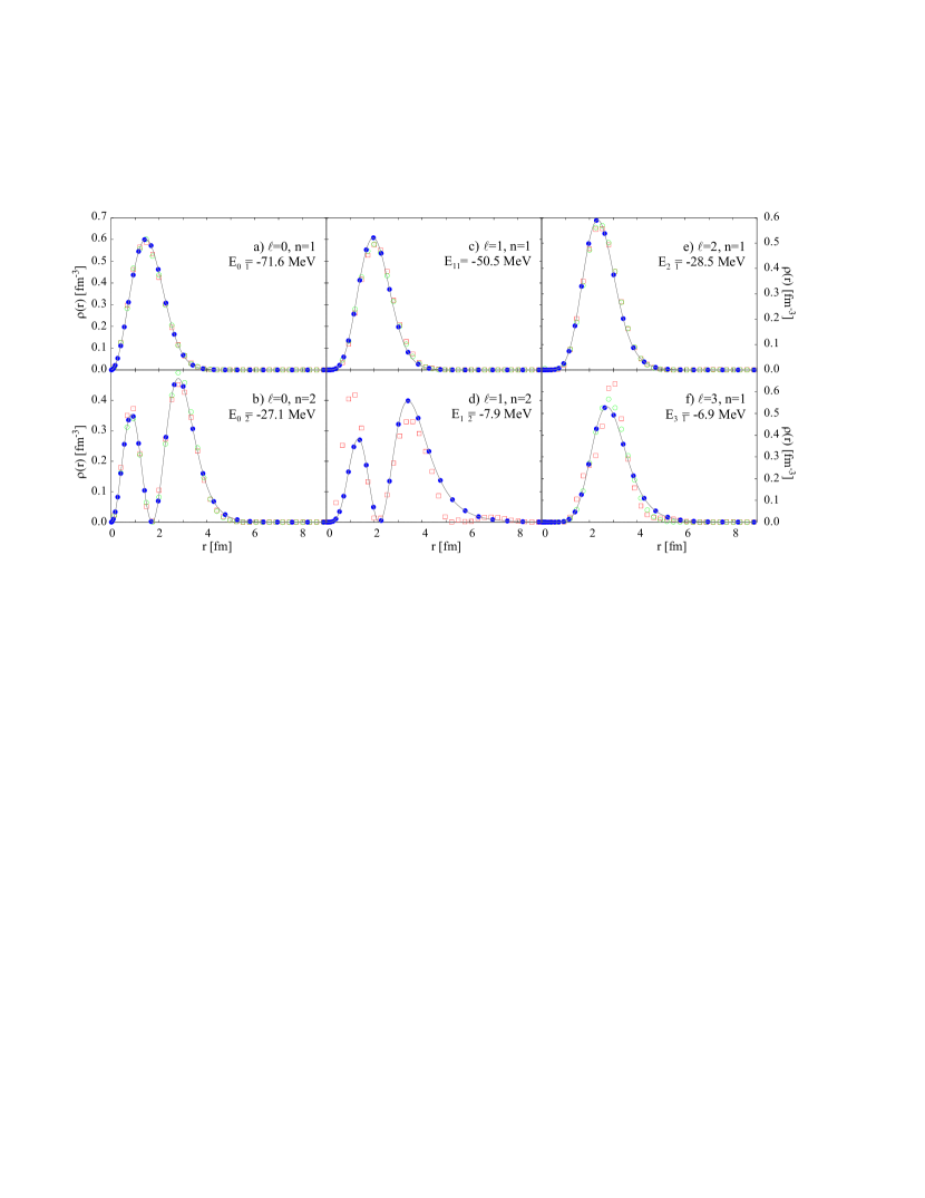
Figure 1: (Color online) Density probabilities $\rho(r)$ of WS bound states, derived using the “exact” shooting method (line), Heisenberg representation in a $\mathcal{HO}$ basis (boxes), CCE using a single $\mathcal{HO}$ basis (empty circles), and CCE using a combination of a $\mathcal{HO}$ and $\mathcal{L}$ basis (filled circles). Where appropriate, the values of the employed parameters were $b=1.4$ fm, and $\gamma=3$ fm^-1. All discrete basis featured $N_{g}=68$ functions, corresponding to the identical number of collocation point for the Gauss-Hermite or Gauss-Laguerre quadrature method, respectively.

We consider a WS potential well with depth $V_{0}=100$ MeV, radius $R=3$ fm, and diffuseness parameter $a=0.6$ fm. In the following we focuss on the calculation of the bound-state energies, and the corresponding probability densities. Numerical results are collected in Table 1 and Figs. 1$a\div f$.

We begin by employing two textbook ref:SSL methods for finding the bound-state eigenvalues of the hamiltonian. Firstly, in order to establish a baseline for our comparison, we employ a shooting technique and solve the radial Schrödinger equation on a grid using the Numerov method. The radial wave function calculation begins at the origin and the numerical solution is stepped out for a fixed energy $E$, to $r_{\mathrm{max}}=12$ fm in $2^{12}\times 10^{3}$ steps. In the presence of an eigenvalue, $E_{n\ell}$, the wave function flips between large negative and positive values for small variations in the energy $E$. The energy $E$ is fine tuned in order to capture this transition. In this limit $E$ tends to $E_{n\ell}$, the true eigenvalue of the Schrödinger equation. For $E=E_{n\ell}$, the numerical wave function becomes normalizable over the radial interval $[0,r_{\mathrm{max}}]$, and we can compute the associated density probability on the interval. These eigenvalues and densities will be referred to as “exact” for the purposes of our numerical comparison.

Secondly, we obtain the solution of the Schrödinger equation in a harmonic oscillator representation, by solving the eigenvalue problem illustrated in Eq. (25) . In this (Heisenberg) picture, the continuum part of the hamiltonian spectrum is inherently discretized. The harmonic oscillator ($\mathcal{HO}$) wave functions depend on the choice of the oscillator parameter $b$, and this in turn introduces a dependence of the calculated spectrum on the oscillator parameter $b$. The corresponding eigenfunctions are linear superpositions of $\mathcal{HO}$ functions, which partially compensates for the fact that the $\mathcal{HO}$ functions do not exhibit the corrected asymptotic behavior demanded by the Wood-Saxon potential. We consider a number of $N_{g}=68$ functions in our $\mathcal{HO}$ expansion, to correspond to the $N_{g}=68$ collocation points used in our Gauss-Hermite quadrature scheme. Test runs for $N_{g}=52$ show that both the bound-state eigenvalues and eigenvectors of this hamiltonian have largely saturated with $N_{g}$, and the subsequent improvements are only minute with increasing $N_{g}>52$. The eigenvalues are very close to the expected exact results. The calculated densities for the lower energy states are reasonably close to the exact result: the more bound the state is, the better the density agreement. For the shallow ($E>-\,10$ MeV) bound-states however, the calculated densities compare poorly with the exact results: the model space is simply too small to allow for a good representation of the wave function, even though the eigenvalue calculation has arguably converged already for this space size.

We turn our attention now to the CCE solution. In Appendix C we list the actual equations we need to solve. In all our CCE calculations the physical vacuum $|\Phi_{n\ell}\rangle$ is represented by the corresponding $\mathcal{HO}_{n\ell}$ wave function. The discrete spectrum of the hamiltonian is then determined one state at a time, by solving the $R$-set of equations described above. In this approach one may hope to account exactly for the existence of the continuum part of the spectrum, by introducing the hole-functions $|\chi_{n\ell}\rangle$ and effectively mapping this continuum onto the bound-state part of the spectrum.

We consider here two qualitatively different scenarios: The first scenario is identical in spirit with the approach used in the recent implementations of the CCE ref:bm_I ; ref:bm_II for spin-isospin shell saturated nuclei: we adopt a one-basis realization of the CCE, where we use the remaining part of the $\mathcal{HO}$ basis (after eliminating those state used to represent the physical vacuum, and possible all other lower energy states of the same symmetry), to construct the desired hole-function $|\chi_{n\ell}\rangle$. The functions in this set are definitely orthogonal to each other, but they do not form a complete basis in the Hilbert space. However, the condition $\langle\phi_{n\ell}|\chi_{n\ell}\rangle=0$ must be satisfied, and indeed the above set of functions is complete in the subspace of all possible $|\chi_{n\ell}\rangle$. However, a simple manipulation of the equations reveals that introducing the hole-function formalism in this picture does not amount to any new information. We are working within the confines of a $\mathcal{HO}$ potential, and no structure outside this space can be built into the desired $|\Psi_{n\ell}\rangle$ eigenfunction of the hamiltonian. We have effectively discretized the continuum, and the accuracy of the calculated eigenvalues and densities is generally close to the results in the Heisenberg picture.

The ground state $[\ell=0,\,n=1]$ has a variational minimum $E_{h}$ for a value $b=1.4$ of the oscillator parameter, and the CCE result in this representation is more sensitive to the choice of $b$ than the previous result in the Heisenberg representation. This reflects the importance of a good choice for the physical vacuum for the CCE: a true variational calculation is necessary to establish the best possible choice of $b$. In reviewing the results, we note on the plus side that this version of the CCE fixes some of the erratic behavior of the density for the $[\ell=3,\,n=1]$ state. Still, we notice that too much strength is pushed into the interior region, as the falloff of the tail is too sharp. On the other hand, the CCE misses completely the second state for $\ell=1$. From table 1 we see that already at the physical vacuum level, the $\mathcal{HO}$ representation is unable to provide an acceptable description of the $[\ell=1,\,n=2]$ state: the vacuum energy $E_{h\equiv\{12\}}$ does not have a minimum for $b\in[1.3,1.5]$, and the subsequent calculation of the hole-function as a linear superposition of $\mathcal{HO}$ functions is unable to remedy this deficiency. Once again, the wrong asymptotic behavior of the $\mathcal{HO}$ functions results into a inadequate representation of the continuum, and thus the serious shortcomings of the CCE in this representation.

In order to establish that this is indeed the case, we consider a second (two-basis) scenario in the CCE. We still represent the physical vacuum as a simple $\mathcal{HO}_{n\ell}$ wave function, but we expand the hole-functions using Laguerre ($\mathcal{L}$) functions as our second complete basis. Unlike the $\mathcal{HO}$ functions which falloff like $\exp[-r^{2}/(2b^{2})]$, the asymptotic behavior of the $\mathcal{L}$ functions has the form $\exp(-\gamma r)$, similarly to the bound-state coulomb functions. Properties of the $\mathcal{L}$ functions are summarized in Appendix D, and for the purpose of this two-set representation of the CCE, we are using a Gauss-Laguerre quadrature scheme with $N_{g}=68$ collocation points.

It is interesting to remark that a CCE calculation done entirely in $\mathcal{L}$ space (similar to the CCE calculation in the $\mathcal{HO}$ space described above), results in good eigenvalues for values of $\gamma=3\div 4$, but fails to generate reasonable densities: if the $\mathcal{HO}$ functions were falling off too quickly with $r$, the $\mathcal{L}$ functions are spread out over large distances and have little usable strength in the interior region which can be used to build the density. When the two basis are combined, however, the CCE results in the two-basis representation literally collapse onto the exact results, for both the bound state energies and densities. The numerical results show very little sensitivity with the value of the oscillator parameter $b$, for a fixed value of $\gamma=3\,\mathrm{fm}^{-1}$: numerical differences for the energies calculated for various values of $b$ appear beyond the six significant digits presented here. The fact that we are working with a finite number ($N_{g}=68$) of basis states is evident as the CCE result is not the same as the exact results, but the error is less than 0.005% .

The CCE calculation has no problem producing accurate energies and densities for the shallow bound states ($E>-\,10$ MeV), and the CCE successfully corrects for the lack of a viable $\mathcal{HO}$ representation in the case of the physical vacuum for the $[\ell=1,\,n=2]$ state. We would argue that a good physical vacuum representation is still important, but a good representation of the continuum is indeed crucial for an accurate calculation of the bound-states spectrum of the hamiltonian.

Table 2: Restoration of normalization of WS eigenfunctions in the CCE: using a pure $\mathcal{HO}$ basis, and a combination of a $\mathcal{HO}$ and $\mathcal{L}$ basis, respectively. All calculations correspond to the values of the parameters $b=1.4$ fm, and $\gamma=3$ fm^-1, respectively.

state	$\langle\Psi|\Psi\rangle_{\mathcal{HO}}$	$\rho_{\mathcal{HO}}$	$\langle\Psi|\Psi\rangle_{\mathcal{HO+L}}$	$\rho_{\mathcal{HO+L}}$
$[\ell=0,\,n=1]$	1.000979	1.0005641	1.000415	1.000000
$[\ell=0,\,n=2]$	1.000011	0.9954375	1.004602	1.000000
$[\ell=1,\,n=1]$	1.000157	0.9988504	1.001309	1.000000
$[\ell=1,\,n=2]$	1.006852	0.9323478	1.081757	1.000000
$[\ell=2,\,n=1]$	1.001492	0.9985834	1.002913	1.000000
$[\ell=3,\,n=1]$	1.000184	0.9823059	1.018200	1.000000

We conclude this analysis by considering the normalization issues we have alluded to at the end of section VI: we remind the reader that the CCE wave function is not normalized in the usual sense, but by requiring $\langle\Phi|\Psi\rangle=1$. Therefore, the observables’ calculation must implicitly “correct” for this artifact, and “restore” the wave function normalization, see Eq. (81). In table 2, we collect the results regarding the normalization of the solution $|\Psi\rangle$, and the normalization of the probability density $\rho(\vec{r})$: for an exact solution of the Schrödinger equation, the density should come out automatically normalized to unity, even though $|\Psi\rangle$ is not. Conversely, the departure from unity in the $\rho(\vec{r})$ normalization, is a test for the quality of the CCE solution. Therefore, it comes to no surprise that the largest discrepancies arise in the normalization of the $[\ell=3,\,n=1]$ and, particularly, $[\ell=1,\,n=2]$ states, in the one-basis $\mathcal{HO}$ representation. The two-basis representation of the CCE on the other hand, performs very well: the density normalization is correct to 11 significant figures.

IX Discussion and Outlook

In this paper we have discussed the fundamental aspects of a new formulation of the coupled-cluster expansion in the continuum, and we have illustrated this approach by considering the simplest ($A=1$) dimensional realization of the many-body problem. For this simple scenario we have derived CCE equations which can be solved either in momentum or coordinate space. We have discussed the calculation of the eigenvalue spectrum of the hamiltonian, as well as the calculation of expectation values of arbitrary operators.

The momentum space approach seems to be the most promising one for future efficient algorithms, with the drawback that an explicit knowledge of the continuum basis states appears to be mandatory: One can use Eqs. (55) and (56) to design an iterative, albeit nonlinear, approach for the direct calculation of the energy, without an explicit reference to the $S_{1}$ correlations. This may allow for a solution based on a nonlinear Monte Carlo approach, contingent upon the favorable resolution of serious concerns related to the numerical convergence and stability, and the feasibility of a practical numerical implementation. This discussion is tied in with the convergence and stability issues of the iterative method outlined in Section VII, following Eq. (88). Work is currently ongoing to solve the technical issues of this numerical approach.

The coordinate space approach is also promising, and likely to offer immediate results. It offers the familiar perspective of a coordinate space implementation, with the added advantage of a lossless account of the continuum part of the single-energy spectrum. This is realized via a small set of hole-functions, labelled after the states which are occupied in the physical vacuum. However, a Monte Carlo approach to solving this set of equations seems difficult to envision at this time: The calculation of the hole-functions employs an expansion in a known (and hopefully finite) basis of functions, with the expansion coefficients obtained as the numerical solution of a system of linear equations derived from Eq. (70).

The stage is now set: We know that in the one-body case, we can derive consistent CCE equations. We will derive next the CCE equations for the deuteron ($A=2$) problem. In the CCE formalism, one has an intermediate level of approximation short of the exact solution, namely the ${\mathbf{S}}_{1}$ and ${\mathbf{S}}_{2}$ levels, respectively. We will solve these equations using the realistic Argonne v₁₈ potential ref:av18 , compare the approximate and exact CCE solutions, and compare with results obtained using other exact methods. In the end, the deuteron problem is extremely simple outside the CCE formalism, since it can be formulated as an one-body problem in terms of the relative coordinate of the system of two nucleons.

Appendix A ($A=1$) commutators

We find useful to write the following anti-commutation properties

$$\{{\mathbf{c}}_{\vec{p}_{1}},{\mathbf{a}}^{\dagger}_{\vec{p}_{2}}\} =\delta_{\vec{p}_{1}\vec{p}_{2}}\>,\qquad\{{\mathbf{c}}_{\alpha},{\mathbf{b}}^{\dagger}_{m_{2}}\}\ =\ 0\>,$$ (90)

$$\{{\mathbf{c}}^{\dagger}_{\alpha},{\mathbf{a}}^{\dagger}_{\vec{p}_{2}}\} =0\>,\qquad\{{\mathbf{c}}^{\dagger}_{n_{1}},{\mathbf{b}}^{\dagger}_{m_{2}}\}\ =\ \delta_{n_{1}m_{2}}\>.$$ (91)

We list now the results used in deriving the CCE equations for our toy single-particle quantum mechanics problem:

• ${\mathbf{c}}^{\dagger}_{\alpha}{\mathbf{c}}_{\beta}$

  $${\mathbf{c}}^{\dagger}_{\alpha}{\mathbf{c}}_{\beta}\ =\ ({\mathbf{a}}^{\dagger}_{\vec{p}_{\alpha}}+{\mathbf{b}}_{n_{\alpha}})({\mathbf{a}}_{\vec{p}_{\beta}}+{\mathbf{b}}^{\dagger}_{n_{\beta}})\>.$$

  We obtain the relevant expectation values

  $$\langle\Phi|{\mathbf{c}}^{\dagger}_{\alpha}{\mathbf{c}}_{\beta}|\Phi\rangle\ =\ \delta_{n_{\alpha}n_{\beta}}\>,$$ (92)

  $$\langle\Phi|{\mathbf{b}}_{n_{b}}{\mathbf{a}}_{\vec{p}_{a}}\ {\mathbf{c}}^{\dagger}_{\alpha}{\mathbf{c}}_{\beta}|\Phi\rangle\ =\ \delta_{\vec{p}_{\alpha}\vec{p}_{a}}\delta_{n_{\beta}n_{b}}\>.$$ (93)

• $[{\mathbf{H}},{\mathbf{S}}_{1}]$

  $$\bigl{[}{\mathbf{c}}^{\dagger}_{\alpha}{\mathbf{c}}_{\beta},\,{\mathbf{a}}^{\dagger}_{\vec{p}_{1}}{\mathbf{b}}^{\dagger}_{n_{1}}\bigr{]}$$

  $$={\mathbf{c}}^{\dagger}_{\alpha}(+\,{\mathbf{b}}_{n_{1}}^{\dagger}\,\delta_{\vec{p_{\beta}}\vec{p_{1}}})+(-\,{\mathbf{a}}_{\vec{p}_{1}}^{\dagger}\,\delta_{n_{\alpha}n_{1}}){\mathbf{c}}_{\beta}$$

  $$=\delta_{\vec{p}_{\beta}\vec{p}_{1}}{\mathbf{c}}^{\dagger}_{\alpha}{\mathbf{b}}^{\dagger}_{n_{1}}-\,\delta_{n_{\alpha}n_{1}}{\mathbf{a}}^{\dagger}_{\vec{p}_{1}}{\mathbf{c}}_{\beta}\>.$$

  Note that

  $$\bigl{[}{\mathbf{c}}^{\dagger}_{\alpha}{\mathbf{c}}_{\beta},\,{\mathbf{a}}^{\dagger}_{\vec{p}_{1}}{\mathbf{b}}^{\dagger}_{n_{1}}\bigr{]}|\Phi\rangle$$

  $$=\Bigl{(}\delta_{\vec{p}_{\beta}\vec{p}_{1}}{\mathbf{c}}^{\dagger}_{\alpha}{\mathbf{b}}^{\dagger}_{n_{1}}-\,\delta_{n_{\alpha}n_{1}}{\mathbf{a}}^{\dagger}_{\vec{p}_{1}}{\mathbf{b}}^{\dagger}_{n_{\beta}}\Bigr{)}\ |\Phi\rangle\>.$$

  Therefore, the relevant expectation values are

  $$\langle\Phi|\bigl{[},\,\bigr{]}|\Phi\rangle\ \doteq\ \delta_{\vec{p}_{\beta}\vec{p}_{1}}\delta_{n_{\alpha}n_{1}}\>,$$ (94)

  $$\langle\Phi|{\mathbf{b}}_{n_{b}}{\mathbf{a}}_{\vec{p}_{a}}\ \bigl{[},\,\bigr{]}|\Phi\rangle$$ (95)

  $$\doteq\delta_{\vec{p}_{\beta}\vec{p}_{1}}\delta_{\vec{p}_{\alpha}\vec{p}_{a}}\delta_{n_{1}n_{a}}-\,\delta_{n_{\alpha}n_{1}}\delta_{\vec{p}_{1}\vec{p}_{a}}\delta_{n_{\beta}n_{b}}\>.$$

• $\bigl{[}[{\mathbf{H}},{\mathbf{S}}_{1}],\,{\mathbf{S}}_{1}\bigr{]}$

  $$\Bigl{[}\bigl{[}{\mathbf{c}}^{\dagger}_{\alpha}{\mathbf{c}}_{\beta},\,{\mathbf{a}}^{\dagger}_{\vec{p}_{1}}{\mathbf{b}}^{\dagger}_{n_{1}}\bigr{]},\,{\mathbf{a}}^{\dagger}_{\vec{p}_{2}}{\mathbf{b}}^{\dagger}_{n_{2}}\Bigr{]}$$

  $$=\delta_{\vec{p}_{\beta}\vec{p}_{1}}(-\,{\mathbf{a}}_{\vec{p}_{2}}^{\dagger}\,\delta_{n_{\alpha}n_{2}}){\mathbf{b}}^{\dagger}_{n_{1}}-\,\delta_{n_{\alpha}n_{1}}{\mathbf{a}}^{\dagger}_{\vec{p}_{1}}(+\,{\mathbf{b}}_{n_{2}}^{\dagger}\,\delta_{\vec{p_{\beta}}\vec{p_{2}}})$$

  $$=-\,\delta_{n_{\alpha}n_{2}}\delta_{\vec{p}_{\beta}\vec{p}_{1}}{\mathbf{a}}^{\dagger}_{\vec{p}_{2}}{\mathbf{b}}^{\dagger}_{n_{1}}-\,\delta_{n_{\alpha}n_{1}}\delta_{\vec{p}_{\beta}\vec{p}_{2}}{\mathbf{a}}^{\dagger}_{\vec{p}_{1}}{\mathbf{b}}^{\dagger}_{n_{2}}\>.$$

  We have

  $$\langle\Phi|\bigl{[}[,\,],\,\bigr{]}|\Phi\rangle\ =\ 0\>,$$ (96)

  $$\langle\Phi|{\mathbf{b}}_{n_{b}}{\mathbf{a}}_{\vec{p}_{a}}\ \bigl{[}[,\,],\,\bigr{]}|\Phi\rangle$$ (97)

  $$\doteq-\,\delta_{n_{\alpha}n_{2}}\delta_{\vec{p}_{\beta}\vec{p}_{1}}\delta_{\vec{p}_{2}\vec{p}_{a}}\delta_{n_{1}n_{b}}-\,\delta_{n_{\alpha}n_{1}}\delta_{\vec{p}_{\beta}\vec{p}_{2}}\delta_{\vec{p}_{1}\vec{p}_{a}}\delta_{n_{2}n_{b}}\>.$$

Appendix B ($A=1$): Equations we need to solve

In general the integral over the continuum particle states must be viewed as an integral over the continuum basis states, plus a sum over the set of discrete states in the spectrum, which remain unoccupied in the physical vacuum $|\Phi\rangle$. For simplicity, in the main body of the paper we assumed that all particle states are located in the continuum and this explicit sum was left out. In this appendix we revisit this issue and list the equivalent of Eqs. (52, 65, 55, 57, 66, 70), for the calculation of the energy and 1$p$1$h$ correlations. We also list the equivalent of Eqs. (75, 76, 79, 80) required for the calculation of observables in momentum and coordinate space.

B.1 Correlations and energies

• Eigenstate of the hamiltonian ${\mathbf{H}}$ :

  $$|\Psi\rangle\ =\ |\phi_{h}\rangle+\sum_{n\neq h}S_{nh}|\phi_{n}\rangle+\int\frac{\mathrm{d}^{3}p}{(2\pi)^{3}}\ S_{\vec{p}h}|\phi_{\vec{p}}\rangle\>,$$ (98)

• Hole-function :

  $$|\chi_{h}\rangle\ =\ |\Psi\rangle-|\phi_{h}\rangle-\sum_{n\neq h}S_{nh}|\phi_{n}\rangle\>.$$ (99)

• $P$-set equations :

  $$E\ =\ \langle\phi_{h}|{\mathbf{H}}|\phi_{h}\rangle+\sum_{n\neq h}\langle\phi_{h}|{\mathbf{H}}|\phi_{n}\rangle\,S_{nh}$$

  $$\qquad\qquad+\int\frac{\mathrm{d}^{3}p}{(2\pi)^{3}}\ \langle\phi_{h}|{\mathbf{H}}|\phi_{\vec{p}}\rangle\,S_{\vec{p}h}\>,$$ (100)

  $$E\,S_{nh}\ =\ \langle\phi_{n}|{\mathbf{H}}|\phi_{h}\rangle+\sum_{n_{1}\neq h}\langle\phi_{n}|{\mathbf{H}}|\phi_{n_{1}}\rangle\,S_{n_{1}h}$$

  $$\qquad\qquad+\int\frac{\mathrm{d}^{3}p_{1}}{(2\pi)^{3}}\ \langle\phi_{n}|{\mathbf{H}}|\phi_{\vec{p}_{1}}\rangle\,S_{\vec{p_{1}}h}\>,$$ (101)

  $$E\,S_{\vec{p}h}\ =\ \langle\phi_{\vec{p}}|{\mathbf{H}}|\phi_{h}\rangle+\sum_{n_{1}\neq h}\langle\phi_{\vec{p}}|{\mathbf{H}}|\phi_{n_{1}}\rangle\,S_{n_{1}h}$$

  $$\qquad\qquad+\int\frac{\mathrm{d}^{3}p_{1}}{(2\pi)^{3}}\ \langle\phi_{\vec{p}}|{\mathbf{H}}|\phi_{\vec{p}_{1}}\rangle\,S_{\vec{p_{1}}h}\>.$$ (102)

• $R$-set equations :

  $$E\ =\ \langle\phi_{h}|{\mathbf{H}}|\phi_{h}\rangle+\langle\phi_{h}|{\mathbf{H}}|\chi_{h}\rangle$$

  $$\qquad\qquad\qquad+\sum_{n\neq h}\langle\phi_{h}|{\mathbf{H}}|\phi_{n}\rangle\,S_{nh}\>,$$ (103)

  $$E\,S_{nh}\ =\ \langle\phi_{n}|{\mathbf{H}}|\phi_{h}\rangle+\langle\phi_{n}|{\mathbf{H}}|\chi_{h}\rangle$$

  $$\qquad\qquad\qquad+\sum_{n_{1}\neq h}\langle\phi_{n}|{\mathbf{H}}|\phi_{n_{1}}\rangle\,S_{n_{1}h}\>,$$ (104)

  $$({\mathbf{H}}-E)\,|\chi_{h}\rangle\ =\$$

  $$\quad-\,({\mathbf{H}}-E)\,\Bigl{[}|\phi_{h}\rangle+\sum_{n_{1}\neq h}|\phi_{n_{1}}\rangle\,S_{n_{1}h}\Bigr{]}\>.$$ (105)

B.2 Observables

• $P$-set complement :

  $$\tilde{S}_{nh}\ =\ S_{nh}\ \Bigl{[}1-\sum_{n_{\neq}h}\tilde{S}_{n_{1}h}S_{n_{1}h}$$ (106)

  $$\qquad\qquad\qquad\qquad-\int\frac{\mathrm{d}^{3}p_{1}}{(2\pi)^{3}}\ \tilde{S}_{\vec{p_{1}}h}S_{\vec{p_{1}}h}\Bigr{]}\>,$$

  $$\tilde{S}_{\vec{p}h}\ =\ S_{\vec{p}h}\ \Bigl{[}1-\sum_{n_{\neq}h}\tilde{S}_{n_{1}h}S_{n_{1}h}$$ (107)

  $$\qquad\qquad\qquad\qquad-\int\frac{\mathrm{d}^{3}p_{1}}{(2\pi)^{3}}\ \tilde{S}_{\vec{p_{1}}h}S_{\vec{p_{1}}h}\Bigr{]}\>,$$

  $$\bar{o}\ =\ \langle\phi_{h}|{\mathcal{O}}|\Psi\rangle$$ (108)

  $$\qquad\quad+\sum_{n\neq h}\tilde{S}_{nh}\Bigl{[}\langle\phi_{n}|{\mathcal{O}}|\Psi\rangle-\langle\phi_{h}|{\mathcal{O}}|\Psi\rangle S_{nh}$$

  $$\qquad\quad+\int\frac{\mathrm{d}^{3}p}{(2\pi)^{3}}\ \tilde{S}_{\vec{p}h}\Bigl{[}\langle\phi_{\vec{p}}|{\mathcal{O}}|\Psi\rangle-\langle\phi_{h}|{\mathcal{O}}|\Psi\rangle S_{\vec{p}h}\Bigr{]}\>.$$

• $R$-set complement :

  $$\tilde{S}_{nh}\ =\ S_{nh}\ \Bigl{[}1-\frac{1}{E}\,\langle\tilde{\chi}_{h}|{\mathbf{H}}|\Psi\rangle$$ (109)

  $$\qquad\qquad\qquad\qquad-\sum_{n_{1}\neq h}\tilde{S}_{n_{1}h}\frac{1}{E}\,\langle\phi_{n_{1}}|{\mathbf{H}}|\Psi\rangle\Bigr{]}\>,$$

  $$\langle\tilde{\chi}_{h}|\ =\ \langle\chi_{h}|\ \Bigl{[}1-\frac{1}{E}\,\langle\tilde{\chi}_{h}|{\mathbf{H}}|\Psi\rangle$$ (110)

  $$\qquad\qquad\qquad\qquad-\sum_{n_{1}\neq h}\tilde{S}_{n_{1}h}\frac{1}{E}\,\langle\phi_{n_{1}}|{\mathbf{H}}|\Psi\rangle\Bigr{]}\>,$$

  $$\bar{o}\ =\ \langle\phi_{h}|{\mathcal{O}}|\Psi\rangle+\langle\tilde{\chi}_{h}|{\mathcal{O}}|\Psi\rangle-\frac{1}{E}\,\langle\tilde{\chi}_{h}|{\mathbf{H}}|\Psi\rangle\langle\phi_{h}|{\mathcal{O}}|\Psi\rangle$$

  $$\qquad+\sum_{n\neq h}\Bigl{[}\langle\phi_{n}|{\mathcal{O}}|\Psi\rangle-\frac{1}{E}\,\langle\phi_{n}|{\mathbf{H}}|\Psi\rangle\langle\phi_{h}|{\mathcal{O}}|\Psi\rangle\Bigr{]}\>.$$ (111)

Appendix C $R$-set practical implementation

Consider two complete sets of functions, $|\phi_{n}\rangle$ and $|\psi_{n}\rangle$. We model the physical vacuum using elements of the first set, while the second set is used to determine the corresponding hole-function. In general, we expect $|\phi_{n}\rangle$ to offer a good description for the interior part of the wave function, while $|\psi_{n}\rangle$ will provide a good description for the tail of the wave function. In practice, we use harmonic oscillator and Laguerre wave functions as the set $|\phi_{n}\rangle$ and the set $|\psi_{n}\rangle$, respectively. Note that a different viable candidate for the second basis may be the set of transformed harmonic oscillator wave functions introduced in ref:SNP , functions which are obtained via a local-scale point transformation of the spherical harmonic oscillator basis. At this time we find the Laguerre functions simpler to handle. Properties of the Laguerre functions are reviewed in Appendix D.

We list now the necessary equations for the ground state. Extension of the formalism to the excited states calculation follows without difficulty. For the ground state, we take $|\Phi\rangle=|\phi_{1}\rangle$. We write the hole-function as an expansion in the second set of functions:

$$|\chi_{1}\rangle\ =\ \sum_{n}\ c_{n}\ |\bar{\psi}_{n}\rangle\>,$$ (112)

with $|\bar{\psi}_{n}\rangle=|\psi_{n}\rangle-|\phi_{1}\rangle\langle\phi_{1}|\psi_{n}\rangle$. Since $|\psi_{n}\rangle$ are not orthogonal to $|\phi_{1}\rangle$, the overlap substraction is necessary to fulfill the condition $\langle\chi_{1}|\phi_{1}\rangle=0$. The price we have to pay is that the set of functions $|\bar{\psi}_{n}\rangle$ are no longer orthogonal to each other. The expansion coefficients $c_{n}$ are found as the solution of the linear system of equations (70) :

$$\sum_{n}\ c_{n}\ \Bigl{[}\langle\bar{\psi}_{m}|{\mathbf{H}}|\bar{\psi}_{n}\rangle\ -\ E\,\langle\bar{\psi}_{m}|\bar{\psi}_{n}\rangle\Bigr{]}\ =\ -\ \langle\bar{\psi}_{m}|{\mathbf{H}}|\phi_{1}\rangle\>,$$ (113)

where

$$\langle\bar{\psi}_{m}|{\mathbf{H}}|\bar{\psi}_{n}\rangle\ =\ \langle\psi_{m}|{\mathbf{H}}|\psi_{n}\rangle+E_{1}\,\langle\psi_{m}|\phi_{1}\rangle\langle\phi_{1}|\psi_{n}\rangle$$ (114)

$$\qquad\qquad-\langle\psi_{m}|\phi_{1}\rangle\langle\phi_{1}|{\mathbf{H}}|\psi_{n}\rangle-\langle\psi_{m}|{\mathbf{H}}|\phi_{1}\rangle\langle\phi_{1}|\psi_{n}\rangle\>,$$

and

$$\langle\bar{\psi}_{m}|\bar{\psi}_{n}\rangle\ =\ \delta_{mn}\ -\ \langle\psi_{m}|\phi_{1}\rangle\langle\phi_{1}|\psi_{n}\rangle\>.$$ (115)

We calculate the ground state energy by using Eq. (66) :

$$E \ =\ \langle\phi_{1}|{\mathbf{H}}|\phi_{1}\rangle\ +\ \sum\ c_{n}\ \langle\phi_{1}|{\mathbf{H}}|\bar{\psi}_{n}\rangle\>,$$ (116)

where

$$\langle\phi_{1}|{\mathbf{H}}|\bar{\psi}_{n}\rangle\ =\ \langle\phi_{1}|{\mathbf{H}}|\psi_{n}\rangle-E_{1}\,\langle\phi_{1}|\psi_{n}\rangle\>.$$ (117)

For the calculation of observables we also need the modified hole-function, $|\tilde{\chi}_{1}\rangle$. Once again we perform an expansion in terms of the set $|\psi_{n}\rangle$. We have

$$|\tilde{\chi}_{1}\rangle\ =\ \sum_{n}\ d_{n}\ |\bar{\psi}_{n}\rangle\>,$$ (118)

where the expansion coefficients are found by solving the linear system of equations (79) :

$$\sum_{n}\ d_{n}\ \Bigl{[}\langle\bar{\psi}_{n}|\bar{\psi}_{m}\rangle+\frac{1}{E}\ \langle\chi_{1}|\bar{\psi}_{m}\rangle\ \langle\bar{\psi}_{n}|{\mathbf{H}}|\Psi\rangle\Bigr{]}=\langle\chi_{1}|\bar{\psi}_{m}\rangle\>.$$ (119)

Subsequently, observables are calculated using Eq. (80). For local operators, it is sufficient to calculate the one-body density

$$\rho(\vec{r}) \ =\ \langle\Psi|\delta(\vec{r}-\vec{r}_{1}|\Psi\rangle/\langle\Psi|\Psi\rangle$$ (120)

$$\ =\ \phi_{1}^{*}(\vec{r})\Psi(\vec{r})\Bigl{[}1-\frac{1}{E}\,\langle\tilde{\chi}_{1}|{\mathbf{H}}|\Psi\rangle\Bigr{]}\ +\ \tilde{\chi}_{1}^{*}(\vec{r})\Psi(\vec{r})\>.$$

Then, the expectation value of an arbitrary one-body local operator $\mathcal{O}$ can be calculated as

$$\langle\Psi|\mathcal{O}(\vec{r})|\Psi\rangle\ =\ \int\mathrm{d}^{3}r_{1}\ \ \mathcal{O}(\vec{r}_{1})\ \langle\Psi|\delta(\vec{r}-\vec{r}_{1}|\Psi\rangle\>.$$ (121)

Appendix D Single-particle wave functions

We briefly review here the properties of the single-particle wave functions employed in the numerical part of this paper. We follow the conventions of Ref. ref:arfken .

• the harmonic oscillator functions have the form

  $$\mathcal{HO}_{n\ell}(x)\ \sim\ x^{\ell+1}e^{-x^{2}/2}\ L_{n}^{\ell+1/2}(x^{2})\>,$$ (122)

  with $x=r/b$, and obey the orthogonality condition

  $$\int_{0}^{\infty}\mathrm{d}r\ \mathcal{HO}_{n\ell}(r)\mathcal{HO}_{m\ell}(r)=\frac{(2n+2\ell+1)!!\sqrt{\pi}}{n!\ b^{3}\ 2^{n+\ell+1}}\ \delta_{nm}\>.$$ (123)

  Here $\{L_{n}^{k}(x)\,;\ n=0,1,\ldots\}$ are the associated Laguerre polynomials.

  For the calculation of the kinetic energy matrix element we will need the identity

  $$\left[\frac{\mathrm{d}^{2}}{\mathrm{d}r^{2}}-\frac{\ell(\ell+1)}{r^{2}}\right]\ \mathcal{HO}_{n\ell}(r)$$ (124)

  $$\ =\ \frac{1}{b^{2}}\ \Bigl{[}2(2n+\ell+\frac{3}{2})-x^{2}\Bigr{]}\ \mathcal{HO}_{n\ell}(x)\>,$$

  and the nonzero elements of the $\langle n\ell|x|m\ell\rangle$ matrix

  $$\langle n\ell|x^{2}|n\ell\rangle\ =\ 2n+\ell+\frac{3}{2}\>,$$ (125)

  $$\langle n-1\ \ell|x^{2}|n\ell\rangle\ =\ -\ \sqrt{n(n+\ell+\frac{1}{2})}\>.$$ (126)

• the Laguerre functions have the form

  $$\mathcal{L}_{n}^{2\ell+2}(x)\ \sim\ x^{\ell+1}e^{-x/2}\ L_{n}^{2\ell+2}(x)\>,$$ (127)

  where $x=\gamma r$, and obey the orthogonality condition

  $$\int_{0}^{\infty}\mathrm{d}x\ \mathcal{L}_{n}^{2\ell+2}(x)\ \mathcal{L}_{m}^{2\ell+2}(x)\ =\ \frac{(n+2\ell+2)!}{n!}\ \delta_{nm}\>.$$

  For the calculation of the kinetic energy matrix element we need the identity

  $$\left[\frac{\mathrm{d}^{2}}{\mathrm{d}x^{2}}-\frac{\ell(\ell+1)}{x^{2}}\right]\ \mathcal{L}_{n}^{2\ell+2}(x)$$ (129)

  $$\ =\ \left(\frac{1}{4}-\frac{n+\ell+1}{x}-\frac{n}{x^{2}}\right)\ \mathcal{L}_{n}^{2\ell+2}(x)$$

  $$\qquad\ +\ \frac{n+2\ell+2}{x^{2}}\ \mathcal{L}_{n-1}^{2\ell+2}(x)\>.$$ (130)

  The above equation involves the unnormalized Laguerre functions. If the normalized Laguerre functions are desired, then the coefficient of $\mathcal{L}_{n-1}^{2\ell+2}$ must be modified accordingly.

  The following identities pertain to the matrix element calculation of $\langle n\ell|x^{-p}|m\ell\rangle$, with $p=1,2$. We have

  $$\int_{0}^{\infty}\mathrm{d}x\ x^{2\ell+1}\ e^{-x}\ L_{n}^{2\ell+2}(x)L_{m}^{2\ell+2}(x)$$ (131)

  $$\ =\ \sum_{c=0}^{\mathrm{min}\{n,m\}}\ \frac{(2\ell+1+c)\,!}{c\,!}\ \>,$$

  and

  $$\int_{0}^{\infty}\mathrm{d}x\ x^{2\ell}\ e^{-x}\ L_{n}^{2\ell+2}(x)L_{m}^{2\ell+2}(x)$$ (132)

  $$\ =\ \sum_{c=0}^{\mathrm{min}\{n,m\}}(n+1-c)(m+1-c)\,\frac{(2\ell+c)\,!}{c\,!}\>.$$

References

- (1) J.R. Bergervoet, P.C. van Campen, R.A.M. Klomp, J.-L. de Kok, T.A. Rijken, V.G.J. Stoks, and J.J. de Swart, Phys. Rev. C 41, 1435 (1990).
- (2) V.G.J. Stoks, R.A.M. Klomp, M.C.M. Rentmeester, and J.J. de Swart, Phys. Rev. C 48, 792 (1993).
- (3) V.G.J. Stoks, R.A.M. Klomp, C.P.F. Terheggen, and J.J. de Swart, Phys. Rev. C 49, 2950 (1994).
- (4) J.L. Friar, G.L. Payne, V.G.J. Stoks, and J.J. de Swart, Phys. Lett. B 311, 4 (1993).
- (5) R. B. Wiringa, V. G. J. Stoks, and R. Schiavilla, Phys. Rev. C 51, 38 (1995).
- (6) R. Machleidt, F. Sammarruca, and Y. Song Phys. Rev. C 53, R1483 (1996).
- (7) R. Machleidt, Phys. Rev. C 63, 024001 (2001).
- (8) D.R. Entem and R. Machleidt, Phys. Lett. B 524, 93 (2003).
- (9) S. C. Pieper, V. R. Pandharipande, R. B. Wiringa, and J. Carlson, Phys. Rev. C 64, 014001 (2001).
- (10) J. Carlson, Phys. Rev. C 36, 2026 (1987).
- (11) S. C. Pieper and R. B. Wiringa, Annu. Rev. Nucl. Part. Sci. 51, 53 (2001), and references therein.
- (12) S.C. Pieper, K. Varga, and R. B. Wiringa, Phys. Rev. C 66, 044310 (2002).
- (13) K.E. Schmidt and S. Fantoni, Phys. Lett. B 446, 99 (1999)
- (14) S. Fantoni, A. Sarsa, and K.E. Schmidt, Phys. Rev. Lett. 87, 181101 (2001)
- (15) H. Kamada et al, Phys. Rev. C 64, 044001 (2002), and references therein.
- (16) P. Navratil, J.P. Vary, and B.R. Barrett, Phys. Rev. Lett. 84, 5728 (2000).
- (17) P. Navratil, J.P. Vary, and B.R. Barrett, Phys. Rev. C 62, 054311 (2000).
- (18) P. Navratil and W.E. Ormand, Phys. Rev. Lett. 88, 152502 (2002), and references therein.
- (19) J. Carlson, V. R. Pandharipande, and R. B. Wiringa, Nucl. Phys. A 401, 59 (1983).
- (20) J. Carlson and R. Schiavilla, Rev. Mod. Phys. 70, 743-841 (1998), and references therein.
- (21) F. Coester, Nucl. Phys. 7, 421 (1958).
- (22) F. Coester and H. Kümmel, Nucl. Phys. 17, 477 (1960).
- (23) H. Kümmel, K. H. Lührmann, and J. G. Zabolitzky, Phys. Rep. 36, 1 (1978).
- (24) R.F. Bishop, Theor. Chim. Acta 80, 95 (1991).
- (25) J. Navarro, R. Guardiola and I. Moliner, Introduction to Modern Methods of Quantum Many-Body Theory and Applications ed A. Fabrocini, S. Fantoni, and E. Krotscheck, Singapore, World Scientific (2002) p 121
- (26) R.F. Bishop, M.F. Flynn, M.C. Bosca, E. Buendia, and R. Guardiola Phys. Rev. C 42, 1341 (1990).
- (27) R. Guardiola, P.I. Moliner, J. Navarro, R.F. Bishop, A. Puente, and N.R. Walet, Nucl. Phys A 609, 218 (1996).
- (28) R.F. Bishop, R. Guardiola, I. Moliner, J. Navarro, M. Portesi, A. Puente, and N.R. Walet, Nucl. Phys A 643, 243 (1998).
- (29) I. Moliner, R.F. Bishop, N.R. Walet, R. Guardiola, J. Navarro, and M. Portesi, Phys. Lett. B 480, 61 (2000).
- (30) I. Moliner, N.R. Walet, and R.F. Bishop, J. Phys. G 28, 1209 (2002).
- (31) J. H. Heisenberg and B. Mihaila, Phys. Rev. C 59, 1440 (1999).
- (32) B. Mihaila and J. H. Heisenberg, Phys. Rev. C 61, 054309 (2000).
- (33) B. Mihaila and J. H. Heisenberg, Phys. Rev. Lett. 84, 1403 (2000).
- (34) I. Sick and J.S. McCarthy, Nucl. Phys. A 150, 631 (1970).
- (35) B. Mihaila and J. H. Heisenberg, Phys. Rev. C 60, 054303 (1999).
- (36) M. Buballa, S. Drozdz, S. Krewald, and J. Speth, Ann. Phys. 208, 346 (1991).
- (37) B. Podolsky, Proc. Natl. Acad. Sci. USA 14, 253 (1928).
- (38) J. L. Friar and S. Fallieros, Phys. Rev. C 29, 232 (1984).
- (39) J. L. Friar and G. L. Payne, Phys. Rev. C 55, 2764 (1997).
- (40) E. W. Schmid, G. Spitz, and W. Lösch, “Theoretical Physics on the Personal Computer,” Springer-Verlag, New York, 1988.
- (41) M. V. Stoitsov, W. Nazarewicz, and S. Pittel, Phys. Rev. C 58, 2092 (1998).
- (42) G. B. Arfken and H. J. Weber, “Mathematical Methods for Physicists,” fourth edition, Academic Press, New York, 1995.