Mean field at finite temperature and symmetry breaking

Abstract

For an infinite system of nucleons interacting through a central spin-isospin schematic force we discuss how the Hartree-Fock theory at finite temperature $T$ yields back, in the $T=0$ limit, the standard zero-temperature Feynman theory when there is no symmetry breaking. The attention is focused on the mechanism of cancellation of the higher order Hartree-Fock diagrams and on the dependence of this cancellation upon the range of the interaction. When a symmetry breaking takes place it turns out that more iterations are required to reach the self-consistent Hartree-Fock solution, because the cancellation of the Hartree-Fock diagrams of order higher than one no longer occurs. We explore in particular the case of an explicit symmetry breaking induced by a constant, uniform magnetic field $B$ acting on a system of neutrons. Here we compare calculations performed using either the single-particle Matsubara propagator or the zero-temperature polarization propagator, discussing under which perturbative scheme they lead to identical results (if $B$ is not too large). We finally address the issue of the spontaneous symmetry breaking for a system of neutrons using the technique of the anomalous propagator: in this framework we recover the Stoner equation and the critical values of the interaction corresponding to a transition to a ferromagnetic phase.

, , and

1 Introduction

In this work we first discuss the problem of the Hartree-Fock (HF) mean field for an infinite system of fermions (nucleons) at finite temperature $T$ in the context of Matsubara theory. In particular we study under which conditions and how the results obtained in the Matsubara framework in the $T\to~{}0$ limit coincide with those of the $T=0$ Feynman theory.

As is well-known, the two formalisms lead to identical results in the absence of symmetry breaking, according to the old theorem for spin one-half fermions of Kohn, Luttinger and Ward (KLW) [1, 2], at least as far as the ground state energy is concerned. Here we extend the theorem to the single-particle propagator (and hence to any one-body observable), aiming at transparently displaying how the cancellation of the diagrams, the mechanism at the basis of KLW, is realized and how the exact $T=0$ limit is retrieved.

Specifically we shall assess quantitatively the magnitude of the diagrams that, while canceling in the $T\to 0$ limit, actually substantially contribute at finite $T$ (not, however, in finite systems [1, 2, 5]). Concerning the size of their contribution to observables like the chemical potential and the magnetization, it turns out to be larger in the proximity of the Fermi temperature $T_{F}$ owing to the temperature dependence of the self-energy. The latter, in fact, displays a marked change near $T_{F}$ reflecting the transition from a quantal to a classical regime. This transition is sensitively affected by the range of the interaction: hence in our study we employ both a finite and a zero-range force, however of schematic nature since we have no pretense of performing a realistic calculation, but rather we aim to investigate the generic temperature behavior of observables that are relevant for the finite temperature physics (such as the chemical potential and the magnetization) in the absence or presence of a symmetry breaking.

We address this last issue in the second part of the paper. When a symmetry is broken then KLW no longer holds and accordingly we explore the impact on the HF field of such an occurrence, both when the breaking is induced explicitly by an external field (as an example we shall consider the case of a constant, uniform magnetic field acting on a system of neutrons) and when it is spontaneous. In the first instance we show how the diagrams that would cancel each other at small temperature in a situation of pure symmetry no longer do so: actually their contribution grows, at $T\to 0$, keeps the value attained at $T=T_{F}$ if the applied magnetic field is large enough.

Moreover, and interestingly, in this situation the successive iterations approach the self-consistent mean field solution smoothly or oscillating around the HF value depending upon the sign of the two-body interaction among neutrons. A ferromagnetic force gently leads to the HF mean field, whereas an antiferromagnetic force entails an approach to the latter oscillating around its value, the magnitude of the oscillations increasing with the strength of the interaction. This behavior contrasts the one occurring in the absence of symmetry breaking where the HF solution is always smoothly reached and, in fact, it is also rapidly reached — at least for a pure exchange interaction (the one we confine ourselves to consider) —at small and large temperature: in the first case because of the KLW theorem, in the second because the large T domain is where quantum physics is gone and classical physics sets in.

The unusual property, referred to above, of the finite temperature HF solutions in presence of a magnetic field $B$ stems in part from the remarkable occurrence that $B$, in breaking the spin rotational symmetry of the system, induces in the interaction matrix element a direct term which otherwise would be absent, the force we employ being of pure exchange character. This is of importance when one aims to recover the vanishing temperature limit of the observables, say the magnetization, computed in the Matsubara HF formalism in the framework of the $T=0$ Feynman theory. This in fact turns out to be possible, in spite of the breakdown of the KLW theorem, using linear response theory, whose applicability is however limited to a specific range of $B$, which we are able to assess quantitatively.

Concerning instead the case of spontaneous symmetry breaking, the non-relativistic quantum field theory describes its occurrence at $T=0$ through the linearization of the equations of motion, i.e. at the mean field level, if the interaction is strong enough [3]. This approach coincides with the many-body Hartree mean field theory at $T=0$, which indeed exhibits a spontaneous breaking of symmetry — again for a force strong enough — provided the variational search for the determinant yielding the minimum energy is allowed to span all of the possible symmetry configurations (we refer to this approach as the generalized $T=0$ HF). This is the path we follow in the last Section in the framework of the anomalous propagator technique [4] at $T=0$.

Likewise, also the temperature HF theory displays a spontaneous symmetry breaking. We prefer, however, to search for the onset of the latter in the framework of the $T=0$ linear response theory which, in parallel to the temperature HF, predicts, either in ring or in the random phase approximation (RPA), a divergent magnetic susceptibility of the Fermi system when the strength of the nucleon-nucleon interaction, assumed to be ferromagnetic, reaches a critical value $V_{\mathrm{crit}}$, thus signaling the occurrence of a phase transition. For a contact interaction, when the response of the system is computed in ring approximation, the value of $V_{\mathrm{crit}}$ thus found is identical to the one obtained in [3] or in the generalized Hartree approximation, whereas the RPA response yields a lower value (by a factor 2/3), which coincides with the one predicted by the $T=0$ generalized HF theory. As mentioned above, the same result is obtained using the thermal single-particle HF propagator, computed with a contact interaction, in the $T\to 0$ limit.

When the symmetry is spontaneously broken, one would like to describe the associated Goldstone modes. In connection with the collective excitations of the system, at zero temperature it turns out that, for an anti-ferromagnetic coupling among the constituents, the Fermi system supports the existence of zero-sound collective modes characterized by a linear relationship between energy and momentum. These modes correspond to the spin waves (also referred to as magnons) found in the antiferromagnetic materials and lower the susceptibility. They represent the Goldstone modes, because our system, although without any cristal structure, still lives in a condensed phase given by the antiferromagnetic order of the spin constituents: we accordingly view the Fermi gas as paramagnetic at finite $T$ and antiferromagnetic at $T=0$.

On the other hand a ferromagnetic interaction only supports the existence of modes embedded in the particle-hole continuum for $V<V_{\mathrm{crit}}$. In this regime such a force softens the response function of the system until, when $V=V_{\mathrm{crit}}$, the latter diverges at zero excitation energy as the transferred momentum becomes very small. Thus the phase transition is also displayed by the behavior of the response function, which basically corresponds to the spin-spin correlation function. On the other hand, for a ferromagnetic coupling $V>V_{\mathrm{crit}}$ new collective modes appear, in the direction orthogonal to the one set by the spontaneous magnetization of the system. These also represent Goldstone modes and will be addressed in a forthcoming paper.

2 Hartree-Fock theory at zero and finite temperature

In this Section we discuss the mean-field HF theory of a system of nucleons at finite temperature. For simplicity we confine ourselves to consider an infinite homogeneous system and a schematic static exchange interaction in the non-relativistic limit.

Figure 1: The perturbative expansion of the HF irreducible self-energy for a pure exchange interaction.

In this situation it is well-known that at zero temperature the HF mean-field theory reduces to first order perturbation theory. Indeed for the single-particle wave functions self-consistency is immediately achieved in the first iteration of the HF equations owing to the translational invariance of the system. In conformity, the diagrams contributing to the HF self-energy (displayed in Fig. 1) vanish, except for the first one: indeed all of them display in the energy variable poles of order $\geq 2$ with zero residue.

For example, considering the diagram (b) of Fig. 1 one has

$$\Sigma^{\star}_{(2)}(\vec{k}) = \left(\frac{i}{\hbar}\right)^{2}\lim_{\eta\to 0^{+}}\int\frac{{\d}\vec{k}_{1}}{(2\pi)^{3}}\int\frac{{\d}\vec{k}_{2}}{(2\pi)^{3}}\int_{-\infty}^{\infty}\frac{{\d}\omega_{1}}{2\pi}\int_{-\infty}^{\infty}\frac{{\d}\omega_{2}}{2\pi}e^{i\omega_{1}\eta}e^{i\omega_{2}\eta}$$ (1)

$$\times V(\vec{k}-\vec{k}_{1})V(\vec{k}_{1}-\vec{k}_{2})[G^{0}(\vec{k}_{1},\omega_{1})]^{2}G^{0}(\vec{k}_{2},\omega_{2}),$$

$V$ being the interaction and $G^{0}$ the zero-order propagator in a Fermi gas with Fermi momentum $k_{F}$. Now, in the frequency integral,

$$I = \int_{-\infty}^{\infty}\frac{{\d}\omega_{1}}{2\pi}e^{i\omega_{1}\eta}[G^{0}(\vec{k}_{1},\omega_{1})]^{2}$$ (2)

$$= \int_{-\infty}^{\infty}\frac{{\d}\omega_{1}}{2\pi}e^{i\omega_{1}\eta}\left[\frac{\theta(|\vec{k}_{1}|-k_{F})}{(\omega_{1}-\omega_{\vec{k}_{1}}+i\eta)^{2}}+\frac{\theta^{(}k_{F}-|\vec{k}_{1}|)}{(\omega_{1}-\omega_{\vec{k}_{1}}-i\eta)^{2}}\right],$$

only the double pole at $\omega_{1}=\omega_{\vec{k}_{1}}+i\eta\equiv\hbar\vec{k}_{1}^{2}/2m+i\eta$ should be considered, the contour of the integration lying in the complex upper plane $\mathrm{Im}~{}\omega_{1}>0$. Hence one gets

$$I=-\eta~{}e^{i(\omega_{\vec{k}_{1}}+i\eta)\eta}\theta(k_{F}-|\vec{k}_{1}|)\rightarrow 0\ \ \mathrm{for}\ \ \eta\rightarrow 0$$ (3)

and likewise for all the other diagrams of Fig. 1 of order $\geq 2$.

On the other hand, at finite temperature the Matsubara diagrams of Fig. 1 no longer vanish. In fact, taking again as an example the second order self-energy, one has

$$\Sigma^{\star}_{(2)}(\vec{k},T) = \left(\frac{-1}{\hbar}\right)^{2}\int\frac{{\d}\vec{k}_{1}}{(2\pi)^{3}}\int\frac{{\d}\vec{k}_{2}}{(2\pi)^{3}}\frac{1}{(\beta\hbar)^{2}}\sum_{n_{1}}\sum_{n_{2}}e^{i\omega_{n_{1}}\eta}e^{i\omega_{n_{2}}\eta}$$ (4)

$$\times V(\vec{k}-\vec{k}_{1})V(\vec{k}_{1}-\vec{k}_{2})[{\mathcal{G}}^{0}(\vec{k}_{1},\omega_{n_{1}})]^{2}{\mathcal{G}}^{0}(\vec{k}_{2},\omega_{n_{2}}),$$

where

$$\mathcal{G}^{0}(\vec{k},\omega_{n})=\frac{1}{i\omega_{n}-(\epsilon_{\vec{k}}^{(0)}-\mu)/\hbar}$$ (5)

is the thermal free propagator at finite $T=1/k_{B}\beta$ ($k_{B}$ being the Boltzmann’s constant and $\mu$ the free chemical potential). Evaluating the frequency sums according to the standard rule

$$\lim_{\eta\to 0^{+}}\sum_{n_{2}}e^{i\omega_{n_{2}}\eta}{\mathcal{G}}^{0}(\vec{k}_{2},\omega_{n_{2}})=\lim_{\eta\to 0^{+}}\sum_{n_{2}}\frac{e^{i\omega_{n_{2}}\eta}}{i\omega_{n_{2}}-(\epsilon^{(0)}_{\vec{k}_{2}}-\mu)/\hbar}=\frac{\beta\hbar}{e^{\beta(\epsilon^{(0)}_{\vec{k}_{2}}-\mu)}+1}$$ (6)

and

$$\lim_{\eta\to 0^{+}}\sum_{n_{1}}e^{i\omega_{n_{1}}\eta}[{\mathcal{G}}^{0}(\vec{k}_{1},\omega_{n_{1}})]^{2} = \lim_{\eta\to 0^{+}}\sum_{n_{1}}\frac{e^{i\omega_{n_{1}}\eta}}{\left[i\omega_{n_{1}}-(\epsilon^{(0)}_{\vec{k}_{1}}-{\mu})/\hbar\right]^{2}}$$ (7)

$$= -\frac{(\beta\hbar)^{2}e^{\beta(\epsilon^{(0)}_{\vec{k}_{1}}-{\mu})}}{\left[e^{\beta(\epsilon^{(0)}_{\vec{k}_{1}}-{\mu})}+1\right]^{2}},$$

where $\omega_{n}=(2n+1)\pi/\beta\hbar$ and the sums run over all the positive and negative integers, one gets

$$\Sigma^{\star}_{(2)}(\vec{k},T) = \frac{-\beta}{\hbar}\int\frac{{\d}\vec{k}_{1}}{(2\pi)^{3}}\int\frac{{\d}\vec{k}_{2}}{(2\pi)^{3}}V(\vec{k}-\vec{k}_{1})V(\vec{k}_{1}-\vec{k}_{2})$$ (8)

$$\times\frac{e^{\beta(\epsilon^{(0)}_{\vec{k}_{1}}-{\mu})}}{\left[e^{\beta(\epsilon^{(0)}_{\vec{k}_{1}}-{\mu})}+1\right]^{2}}\frac{1}{e^{\beta(\epsilon^{(0)}_{\vec{k}_{2}}-\mu)}+1}.$$

The self-energy (8) does not vanish: as a consequence, at finite $T$, even for an infinite system, the HF equations are not trivial.

We briefly illustrate this point using, as an example, a simple static spin-isospin dependent nucleon-nucleon central interaction of the type

$$V=\vec{\sigma}_{1}\cdot\vec{\sigma}_{2}\vec{\tau}_{1}\cdot\vec{\tau}_{2}v({\vec{x}}_{1}-{\vec{x}}_{2})$$ (9)

which, of course, has no pretense of being realistic.

Since the system is homogeneous, the eigenfunctions are still plane waves, whereas the HF eigenvalues read

$$\epsilon_{\vec{k}}=\epsilon_{\vec{k}}^{(0)}+\hbar\Sigma^{\star}_{\mathrm{HF}}(\vec{k},T),$$ (10)

where

$$\hbar\Sigma^{\star}_{\mathrm{HF}}(\vec{k},T)=-9\int\frac{{\d}\vec{k}^{\prime}}{(2\pi)^{3}}n_{\vec{k}^{\prime}}v(\vec{k}-\vec{k}^{\prime})$$ (11)

is the HF irreducible self energy for the interaction (9),

$$n_{\vec{k}}=\frac{1}{e^{\beta(\epsilon_{\vec{k}}-\mu)}+1}$$ (12)

the Fermi distribution and $v(\vec{k})$ the Fourier transform of $v(\vec{x})$.

Thus the HF equations at finite temperature, unlike the case at $T=0$, represent a non trivial self-consistency problem, because the single-particle energies (the eigenvalues) enter not only in the equations, but in the Fermi distribution as well.

Accordingly, the system of equations

$$\epsilon_{\vec{k}} = \epsilon_{\vec{k}}^{(0)}+\hbar\Sigma^{\star}_{\mathrm{HF}}(\vec{k},T)$$ (13a)

$$\rho = 4\displaystyle{\int\frac{{\d}\vec{k}^{\prime}}{(2\pi)^{3}}n_{\vec{k}^{\prime}}},$$ (13b)

where the density $\rho$ of the system is assumed to be fixed, should be solved. We have accomplished this task through numerical iterations of the above equations (the unknowns being $\epsilon_{\vec{k}}$ and $\mu$) until reaching self-consistency (see Subsection 2.3 for the numerical results).

At zero order $\epsilon_{\vec{k}}\equiv\epsilon_{\vec{k}}^{(0)}$ and one fixes $\mu\equiv\mu^{(0)}$ through Eq. (13b), i. e.

$$\rho=4\int\frac{{\d}\vec{k}^{\prime}}{(2\pi)^{3}}\frac{1}{e^{\beta(\epsilon_{\vec{k}^{\prime}}^{(0)}-\mu^{(0)})}+1}.$$ (14)

At first order, from (13a) one has

$$\epsilon_{\vec{k}}^{(1)}=\epsilon_{\vec{k}}^{(0)}-9\int\frac{{\d}\vec{k}^{\prime}}{(2\pi)^{3}}n_{\vec{k}^{\prime}}^{(0)}v(\vec{k}-\vec{k}^{\prime}),$$ (15)

with $n_{\vec{k}^{\prime}}^{(0)}=1/\exp[\beta(\epsilon_{\vec{k}^{\prime}}^{(0)}-\mu^{(0)})+1]$; from (13b) one then has

$$\rho=4\int\frac{{\d}\vec{k}^{\prime}}{(2\pi)^{3}}\frac{1}{e^{\beta(\epsilon_{\vec{k}^{\prime}}^{(1)}-\mu^{(1)})}+1},$$ (16)

which fixes a new chemical potential $\mu^{(1)}$. The latter is then put back in (13a) together with $\epsilon_{\vec{k}}^{(1)}$ in order to generate $\epsilon_{\vec{k}}^{(2)}$ and so on.

Numerically the procedure is quite straightforward. However, it is of interest to analyze its diagrammatic content, since it helps to understand the different roles played by the various classes of diagrams at zero and finite temperature.

Thus — following the steps outlined above for the solution of the HF equations — the first order self-energy $\Sigma_{(1)}^{\star}$ is displayed in Fig. 2a: it embodies $\mu^{(0)}$, the chemical potential for the non-interacting system. $\Sigma_{(1)}^{\star}$, together with $\mu^{(1)}$ — the new chemical potential determined by the requirement of fixed density, Eq. (16) — is then inserted into the Dyson equation for the thermal propagator, namely

$$\mathcal{G}(\vec{k},\omega_{n})=\mathcal{G}^{0}(\vec{k},\omega_{n})+\mathcal{G}^{0}(\vec{k},\omega_{n})\Sigma^{\star}(\vec{k},T)\mathcal{G}(\vec{k},\omega_{n})$$ (17)

whose solution is (Fig. 2b)

$$\mathcal{G}_{D_{1}}(\vec{k},\omega_{n})=\frac{1}{i\omega_{n}-(\epsilon_{\vec{k}}^{(0)}+\hbar\Sigma^{\star}_{(1)}(\vec{k},T)-\mu^{(1)})/\hbar}.$$ (18)

Figure 2: The thermal first order self-energy (panel a) and the perturbative expansion of the thermal first-iteration HF propagator (panel b).

Fig. 2b clearly illustrates that the chemical potential associated with the external propagation lines or with those linking different self-energy insertions should now not be $\mu^{(0)}$, but rather $\mu^{(1)}$, in order to keep the density of the system constant.

One then computes with the propagator (18) the new self-energy $\Sigma^{\star}_{D_{1}}(\vec{k},T)$, which will embody the HF diagrams shown in Fig. 3a and will be used to fix a new chemical potential $\mu^{(2)}$.

Then, solving the Dyson equation with $\Sigma^{\star}_{D_{1}}(\vec{k},T)$ as a kernel will obviously lead to the new propagator shown in Fig. 3b. The procedure should be iterated until self-consistency is reached. Through this iterative procedure all the HF diagrams are generated and naturally organized in different classes.

Figure 3: Perturbative expansion of the first iteration irreducible HF thermal self-energy (panel a) and of the second-iteration HF thermal propagator (panel b).

2.1 The case of a zero-range interaction

As a preliminary we address the HF problem at finite $T$ considering the simple case of a zero-range interaction of pure exchange nature, namely we set in (9)

$$v(\vec{x}_{1}-\vec{x}_{2})=V_{1}\delta(\vec{x}_{1}-\vec{x}_{2}),$$ (19)

whose Fourier transform is of course just $V_{1}$.

The HF equations (13) in this case reduce to:

$$\left\{\begin{array}[]{rl}\epsilon_{\vec{k}}&=\epsilon_{\vec{k}}^{(0)}-9V_{1}\displaystyle{\int\frac{{\d}\vec{k}^{\prime}}{(2\pi)^{3}}}\frac{1}{e^{\beta(\epsilon_{\vec{k}^{\prime}}-\mu)}+1}\\ \rho&=4\displaystyle{\int\frac{{\d}\vec{k}^{\prime}}{(2\pi)^{3}}}\frac{1}{e^{\beta(\epsilon_{\vec{k}^{\prime}}-\mu)}+1}.\end{array}\right.$$ (20)

At zero-order $\epsilon_{\vec{k}}=\epsilon_{\vec{k}}^{(0)}$ and the chemical potential $\mu^{(0)}$ (a few terms of its expansion as a function of $k_{F}$ and $T$ are quoted in Appendix A) is fixed by the requirement of yielding the correct density (see Eq. (14)).

By inserting these results into Eq. (20) we get

$$\epsilon_{\vec{k}}^{(1)} = \epsilon_{\vec{k}}^{(0)}+\hbar\Sigma^{\star}_{(1)}$$ (21)

$$= \epsilon_{\vec{k}}^{(0)}-9V_{1}\int\frac{{\d}\vec{k}^{\prime}}{(2\pi)^{3}}\frac{1}{e^{\beta(\epsilon_{\vec{k}^{\prime}}^{(0)}-\mu^{(0)})}+1}$$

$$= \epsilon_{\vec{k}}^{(0)}-\frac{9}{4}V_{1}\rho.$$

Again, the chemical potential has now to be redefined in order to keep the density constant (see Eq. (16)). It is immediately seen that in the present case of a zero-range interaction the change of $\mu$ amounts to a mere constant shift, i.e.

$$\mu^{(1)}=\mu^{(0)}-\frac{9}{4}V_{1}\rho.$$ (22)

Performing then a second iteration we obtain

$$\epsilon_{\vec{k}}^{(2)} = \epsilon_{\vec{k}}^{(0)}+\hbar\Sigma^{\star}_{D_{1}}(\vec{k})$$ (23)

$$= \epsilon_{\vec{k}}^{(0)}-9V_{1}\int\frac{{\d}\vec{k}^{\prime}}{(2\pi)^{3}}\frac{1}{e^{\beta(\epsilon_{\vec{k}^{\prime}}^{(1)}-\mu^{(1)})}+1}$$

$$= \epsilon_{\vec{k}}^{(0)}-\frac{9}{4}V_{1}\rho=\epsilon_{\vec{k}}^{(1)},$$

where $\hbar\Sigma^{\star}_{D_{1}}$ is here computed using the propagator (18), which, for a zero-range interaction, reads

$$\mathcal{G}_{D_{1}}(\vec{k},\omega_{n})=\frac{1}{i\omega_{n}-(\epsilon_{\vec{k}}^{(0)}-9V_{1}\rho/4-\mu^{(1)})/\hbar}.$$ (24)

Since Eq. (23) clearly entails the identity

$$\hbar\Sigma^{\star}_{(1)}=\hbar\Sigma^{\star}_{D_{1}},$$ (25)

without any depence on $T$, we conclude that self-consistency is immediately achieved at any temperature for a zero-range force. In other words, for such an interaction the HF problem is trivial both at $T=0$ and at finite $T$.

The diagrammatic content of Eq. (25), displayed in Fig. 4, helps in understanding this conclusion: in fact, Eq. (25) holds valid because the diagrams on the right hand side of Fig. 4 cancel at any temperature order by order in the coupling constant $V_{1}$. Note that $V_{1}$ appears both in the interaction lines and in the chemical potential $\mu^{(1)}$: hence even the diagram (a) in Fig. 4 contributes to all orders in $V_{1}$.

Figure 4: Diagrammatic representation of the equation $\Sigma^{\star}_{(1)}=\Sigma^{\star}_{D_{1}}$

.

To illustrate analytically these cancellations we evaluate diagram (a) to the order $O(V_{1}^{3})$ using Eq. (22). We get

$$\Sigma^{\star(a)}_{D_{1}} = -9\frac{V_{1}}{\hbar}\int\frac{{\d}\vec{k}}{(2\pi)^{3}}\frac{1}{e^{\beta(\epsilon_{\vec{k}}^{(0)}-\mu^{(1)})}+1}$$ (26)

$$= -9\frac{V_{1}}{\hbar}\int\frac{{\d}\vec{k}}{(2\pi)^{3}}\frac{1}{e^{\beta(\epsilon_{\vec{k}}^{(0)}-\mu^{(0)})}+1}e^{-9\beta V_{1}\rho/4}$$

$$\qquad\times\left[1+\frac{\sum_{n=1}^{\infty}(-9\beta V_{1}\rho/4)^{n}/n!}{e^{\beta(\epsilon_{\vec{k}}^{(0)}-\mu^{(0)})}+1}\right]^{-1}$$

$$= -\frac{9}{4}\frac{V_{1}}{\hbar}\rho+(9V_{1})^{2}\frac{\beta\rho}{4\hbar}\int\frac{{\d}\vec{k}}{(2\pi)^{3}}\frac{e^{\beta(\epsilon_{\vec{k}}^{(0)}-\mu^{(0)})}}{\left[e^{\beta(\epsilon_{\vec{k}}^{(0)}-\mu^{(0)})}+1\right]^{2}}+O\left(V_{1}^{3}\right).$$

From the above one sees that on the right hand side of Eq. (25) the term linear in $V_{1}$ cancels with the left hand side, whereas the quadratic term cancels with the leading order term in $V_{1}$ associated with the diagram (b). Indeed, computing the latter at the lowest order, that is with $\mu^{(0)}$ in all the propagation lines, one obtains

$$\Sigma^{\star(b)}_{D_{1}} = (9V_{1})^{2}\left(-\frac{1}{\beta\hbar^{2}}\right)^{2}\int\frac{{\d}\vec{k}}{(2\pi)^{3}}\int\frac{{\d}\vec{k}^{\prime}}{(2\pi)^{3}}\sum_{n^{\prime}=-\infty}^{\infty}\frac{e^{i\omega_{n^{\prime}}\eta^{\prime}}}{i\omega_{n^{\prime}}-(\epsilon_{\vec{k}^{\prime}}^{(0)}-\mu^{(0)})/\hbar}$$ (27)

$$\quad\times\sum_{n=-\infty}^{\infty}\frac{e^{i\omega_{n}\eta}}{\left(i\omega_{n}-(\epsilon_{\vec{k}}^{(0)}-\mu^{(0)})/\hbar\right)^{2}}+O\left(V_{1}^{3}\right).$$

Performing then the sums over the Matsubara frequencies with the usual contour integration techniques as in Eq. (7), one gets a contribution precisely canceling the term quadratic in $V_{1}$ in Eq. (26). By the same arguments the cancellation is proved to hold at any order in $V_{1}$. In the following we shall refer to this occurrence equivalently as the cancellation theorem or the KLW theorem.

2.2 The case of a finite-range interaction

We now show that the cancellation mechanism previously illustrated occurs (under certain conditions of symmetry) also for a finite range potential, but, strictly speaking, in the limit $T\to 0$ only.

For this purpose let

$$v({\vec{x}}_{1}-{\vec{x}}_{2})=V_{1}\frac{\lambda^{2}}{4\pi}\frac{e^{-\lambda|{\vec{x}}_{1}-{\vec{x}}_{2}|}}{|{\vec{x}}_{1}-{\vec{x}}_{2}|},$$ (28)

which yields back the zero-range force in the $\lambda\to\infty$ limit and whose Fourier transform is

$$v(k)=V_{1}\frac{\lambda^{2}}{\lambda^{2}+k^{2}}$$ (29)

(note that in the figures we shall express the range parameter $\lambda$ in MeV). The first order self-energy is then easily obtained and reads

$$\Sigma^{\star}_{(1)}(\vec{k},T)=-9\frac{V_{1}}{\hbar}\frac{\lambda^{2}}{(2\pi)^{2}}\frac{1}{2k}\int_{0}^{\infty}{\d}k_{1}k_{1}\ln\frac{\lambda^{2}+(k+k_{1})^{2}}{\lambda^{2}+(k-k_{1})^{2}}\frac{1}{e^{\beta(\epsilon_{\vec{k}_{1}}^{(0)}-\mu^{(0)})}+1}.$$ (30)

In the $T\to 0$ limit, where the Fermi distribution reduces to a $\theta$ function, the integration in Eq. (30) can be done analytically, yielding

$$\Sigma^{\star}_{(1)}(\vec{k},T=0) = -9\frac{V_{1}}{\hbar}\frac{\lambda^{3}}{(2\pi)^{2}}\left[\frac{k_{F}}{\lambda}-\left(\arctan\frac{k_{F}-k}{\lambda}+\arctan\frac{k_{F}+k}{\lambda}\right)+\right.$$ (31)

$$\qquad\left.+\frac{1}{4}\left(\frac{k_{F}^{2}}{\lambda k}-\frac{k}{\lambda}+\frac{\lambda}{k}\right)\ln\frac{1+(k_{F}+k)^{2}/\lambda^{2}}{1+(k_{F}-k)^{2}/\lambda^{2}}\right].$$

At second order one gets

$$\Sigma^{\star}_{(2)}(\vec{k},T) = \frac{-\beta}{\hbar}\left(9V_{1}\frac{\lambda^{2}}{(2\pi)^{2}}\right)^{2}\frac{1}{4k}\int_{0}^{\infty}{\d}k_{1}\int_{0}^{\infty}{\d}k_{2}k_{2}\ln\frac{\lambda^{2}+(k+k_{1})^{2}}{\lambda^{2}+(k-k_{1})^{2}}$$ (32)

$$\times\ln\frac{\lambda^{2}+(k_{1}+k_{2})^{2}}{\lambda^{2}+(k_{1}-k_{2})^{2}}\frac{e^{\beta(\epsilon^{(0)}_{k_{1}}-\mu^{(1)})}}{\left(e^{\beta(\epsilon^{(0)}_{k_{1}}-\mu^{(1)})}+1\right)^{2}}\frac{1}{e^{\beta(\epsilon^{(0)}_{k_{2}}-\mu^{(0)})}+1}.$$

The above can be obtained from Eq. (8), provided one inserts $\mu=\mu^{(0)}$ in the innermost propagator and $\mu=\mu^{(1)}$ elsewhere, according to the previous discussion (see Fig. 3a).

Eq. (32) contains a Fermi distribution and a factor which is proportional to the derivative of a Fermi distribution with respect to the energy $\epsilon^{(0)}_{\vec{k}_{1}}$. These, in the limit of $T\to 0$, yield a theta function, $\theta(\mu^{(0)}-\epsilon^{(0)}_{\vec{k}_{2}})$, and a $\delta$ distribution, $\delta(\mu^{(1)}-\epsilon^{(0)}_{\vec{k}_{1}})$, respectively. Thus also $\Sigma^{\star}_{(2)}$, in this limit, can be analytically expressed as

$$\Sigma^{\star}_{(2)}(\vec{k},T=0)=-\frac{1}{\hbar^{2}}\left(9V_{1}\frac{\lambda^{2}}{(2\pi)^{2}}\right)^{2}\frac{1}{8k}\sqrt{\frac{m}{2\mu^{(1)}}}$$

$$\qquad\times\ln\left[\frac{\lambda^{2}+\left(k+\sqrt{2m\mu^{(1)}}/\hbar\right)^{2}}{\lambda^{2}+\left(k-\sqrt{2m\mu^{(1)}}/\hbar\right)^{2}}\right]\Biggl{[}4\frac{\sqrt{2m\mu^{(1)}}}{\hbar}k_{F}+4\frac{\sqrt{2m\mu^{(1)}}}{\hbar}$$

$$\qquad\times\lambda\left(\arctan\frac{\sqrt{2m\mu^{(1)}}/\hbar-k_{F}}{\lambda}-\arctan\frac{\sqrt{2m\mu^{(1)}}/\hbar+k_{F}}{\lambda}\right)$$

$$\qquad+\left(k_{F}^{2}-\frac{2m\mu^{(1)}}{\hbar^{2}}+\lambda^{2}\right)\ln\frac{\lambda^{2}+\left(\sqrt{2m\mu^{(1)}}/\hbar+k_{F}\right)^{2}}{\lambda^{2}+\left(\sqrt{2m\mu^{(1)}}/\hbar-k_{F}\right)^{2}}\Biggr{]}$$ (33)

and is not vanishing. Nevertheless, also for finite range forces self-consistency is immediately achieved for $T\to 0$.

The proof proceeds along the lines followed in the case of a zero-range interaction. Indeed, since the chemical potential at first order is given by

$$\mu^{(1)} = \mu^{(0)}+\hbar\Sigma^{\star}_{(1)}(k_{F},T=0)$$ (34)

$$= \mu^{(0)}-9V_{1}\frac{\lambda^{2}k_{F}}{(2\pi)^{2}}\left(1-\frac{\lambda}{k_{F}}\arctan\frac{2k_{F}}{\lambda}+\frac{\ln\left(1+4k_{F}^{2}/\lambda^{2}\right)}{4k_{F}^{2}/\lambda^{2}}\right),$$

we can compute, through the same power expansion illustrated in Eq. (26), the diagram (a) of Fig. 4 to the order $O\left(V_{1}^{3}\right)$, getting

$$\Sigma^{\star}_{D_{1}}(\vec{k},T=0)=\Sigma^{\star}_{(1)}(\vec{k},T=0)+\frac{1}{\hbar^{3}}\left[9V_{1}\frac{\lambda^{2}}{(2\pi)^{2}}\right]^{2}\frac{mk_{F}}{2k}$$

$$\quad\times\left[1-\frac{\lambda}{k_{F}}\arctan\frac{2k_{F}}{\lambda}+\frac{\ln\left(1+4k_{F}^{2}/\lambda^{2}\right)}{4k_{F}^{2}/\lambda^{2}}\right]\ln\frac{\lambda^{2}+(k+k_{F})^{2}}{\lambda^{2}+(k-k_{F})^{2}}+O(V_{1}^{3}).$$

We thus see that the second term on the right hand side of the above equation exactly cancels the contribution of order $V_{1}^{2}$ arising from the diagram (b) of Fig. 4, whose analytic expression is given by Eq. (2.2) computed with $\mu^{(0)}=\hbar^{2}k_{F}^{2}/2m$ and replacing $\mu^{(1)}$ with $\mu^{(0)}$ in all places, i.e. in all the propagation lines. This is the essence of the cancellation theorem.

Somewhat surprisingly the validity of the latter actually extends over a remarkably large range of temperatures, as it appears from the numerical results reported in Subsection 2.3.

2.3 Numerical results

We now present a few numerical results to assess quantitatively the role of the higher order perturbative HF diagrams at finite $T$ and the behavior of the chemical potential as a function of temperature and density. We also explore the sensitivity of our outcomes to the values of the parameters characterizing our schematic interaction.

Specifically, we compute:

• the temperature behavior of the self-consistent HF chemical potential $\mu_{\mathrm{HF}}$ at a fixed density for various strengths and ranges of the force (Fig. 6);

• the size of the difference $\mu^{(i)}-\mu^{(i+1)}$ between the successive iterations leading to the HF chemical potential, as a function of $T$ to asses the impact of the higher order perturbative terms on $\mu_{\mathrm{HF}}$ (Fig. 6);

• the temperature dependence of the first and second order contributions to the HF self-energy (Fig. 7).

• the temperature and density dependence of $\mu^{(0)}-\mu_{\mathrm{HF}}$ for a given interaction (Fig. 8);

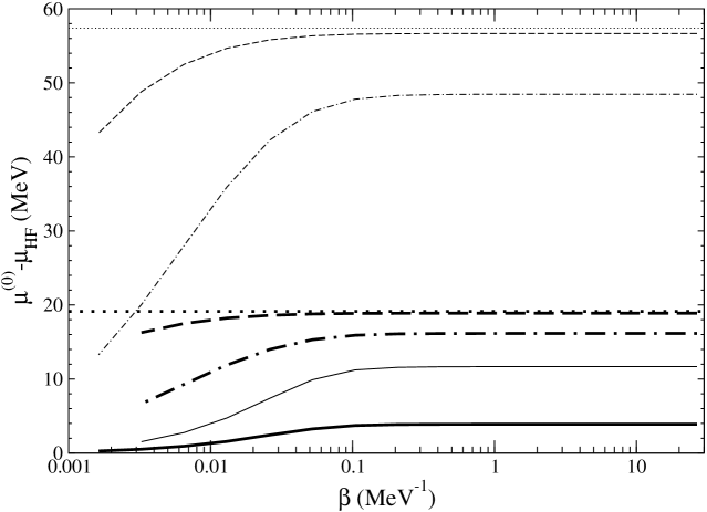
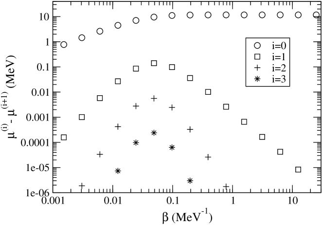
Figure 5: The difference $\mu^{(0)}-\mu_{\mathrm{HF}}$ as a function of $\beta$ for the cases of a force of zero-range (dotted) and finite range: $\lambda=3000$ MeV (dashed), $\lambda=770$ MeV (dot-dashed), $\lambda=140$ MeV (solid). The light lines refer to a strength $V_{1}=150$ MeV fm³, the heavy ones to $V_{1}=50$ MeV fm³. The density is $\rho=0.17$ nucleons/fm³.

Figure 6: The differences $\mu^{(i)}-\mu^{(i+1)}$, computed in HF at finite $T$, as function of $\beta$ in the case of a finite range interaction with $\lambda=140$ MeV and $V_{1}=150$ MeV fm³. Note that the peak of the curves essentially corresponds to the Fermi temperature.

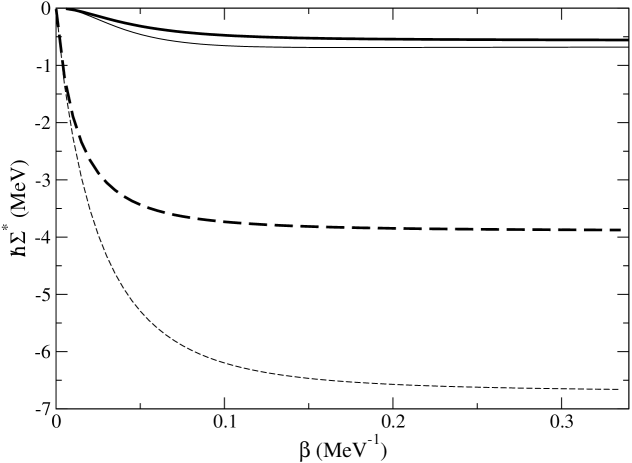
Figure 7: $\hbar\Sigma^{\star}_{(1)}$ (dashed) and $\hbar\Sigma^{\star}_{(2)}$ (solid) as a function of $\beta$ with $\lambda=140$ MeV and $V_{1}=50$ MeV fm³ for two different values of $k$: $k=0$ (light lines) and $k=k_{F}=1.36$ fm${}^{-}1$ (heavy lines).

Figure 8: $\mu^{(0)}-\mu_{\mathrm{HF}}$ as a function of $\beta$ and $\rho$ for a finite range force with $\lambda=140$ MeV and $V_{1}=150$ MeV fm³.

In Fig. 6 the HF chemical potential is seen to be simply shifted from the non-interacting value $\mu^{(0)}$ by a constant amount over a wide range of temperature, as it happens for a zero-range interaction.

Notably this shift turns out to be essentially given by the first order proper self-energy computed, for $T=0$, at the Fermi surface. Since $\hbar\Sigma^{\star}_{(1)}$ turns out to be remarkably stable with the temperature (see Fig. 7), we infer that the cancellation theorem, strictly valid only in the $T\to 0$ limit, actually remains operative over a quite large range of temperatures, almost until the Fermi temperature. This is defined as

$$k_{B}T_{F}=\epsilon_{F}=\frac{1}{\beta_{F}}$$ (36)

and one has $k_{B}T_{F}=34.48$ MeV ($\beta_{F}=0.029$ MeV^-1) for the interaction in Eq. (28) with $\lambda=140$ MeV and $V_{1}=50$ MeV fm³ and $k_{B}T_{F}=26.7$ MeV ($\beta_{F}=0.037$ MeV^-1) for the same interaction, but with $V_{1}=150$ MeV fm³.

We then conclude that for temperatures up to the proximity of $T_{F}$ the chemical potential is

$$\mu_{\mathrm{HF}}=\epsilon_{F}^{(0)}+\hbar\Sigma^{\star}_{(1)}(k=k_{F},T=0),$$ (37)

as follows by comparing the $T\to 0$ limit of the self-energy shown in Fig. 7 (heavy dashed line) with the absolute value for large $\beta$ (3.89 MeV) of the heavy solid line in Fig. 6, which expresses $\mu^{(0)}-\mu_{\mathrm{HF}}$.

It is also evident in Fig. 6 that $\mu_{\mathrm{HF}}$ goes to $\mu^{(0)}$ for small values of $\beta$ (classical limit), as it should, since here all the Feynman diagrams vanish. In fact, our exchange interaction is of purely quantum nature and, as such, is bound to vanish at large temperature. This behavior is also transparent in Fig. 7.

The findings of Fig. 6 are complemented by those of Fig. 6, which conveys the information on the number of iterations required to achieve self-consistency. The figure shows that higher order iterations (i.e. diagrams) become significant for $T$ approaching $T_{F}$, the temperature separating the classical from the quantum regime. This outcome illustrates the significance of $T_{F}$: in fact, a degenerate normal Fermi system, namely with a well-defined Fermi surface, lives in the temperature range $T<T_{F}$. Accordingly, the impact of the Fock’s diagrams of order larger than one — that tend to disrupt the Fermi surface — become appreciable precisely at the Fermi temperature. Away from $T_{F}$ their contribution is gradually disappearing both for $T\to 0$ and $T\to\infty$ but, as previously discussed, for two radically different reasons, i. e. the cancellation theorem and the classical behavior (all the diagrams going to zero), respectively. Hence, for small $T$ the first iteration provides an almost exact estimate of the self-energy, in spite of the fact that, as we can clearly see in Fig.7, $\hbar\Sigma^{\star}_{(2)}$, far from vanishing at small values of $T$, approaches the asymptotic limit given by Eq. (2.2).

In concluding this Section we offer a global view of the behavior of $\mu^{(0)}-\mu_{\mathrm{HF}}$ as a function of both $\beta$ and $\rho$ in Fig. 8, where the features of the chemical potential above discussed clearly appear.

3 Propagation in presence of an induced symmetry breaking: the case of the external magnetic field

In this Section we address the problem of the relationship between the Matsubara and Feynman theories at $T=0$ in the presence of a dynamically induced symmetry breaking. In this situation the two theories provide different results [5], the correct ones being given by Matsubara. We revisit this issue first for the well-known example of a non-interacting system of neutrons placed in an external constant and uniform magnetic field pointing into the $z$-direction, whose second-quantized hamiltonian reads

$$\hat{H}=\int{\d}\vec{x}\hat{\Psi}^{\dagger}_{\alpha}(\vec{x})\left[\delta_{\alpha\beta}\left(-\frac{\hbar^{2}\nabla^{2}}{2m}\right)+V_{\alpha\beta}(\vec{x})\right]\hat{\Psi}_{\beta}(\vec{x}),$$ (38)

where

$$V_{\alpha\beta}=-\mu_{0}~{}\vec{B}\cdot\vec{\sigma}_{\alpha\beta}=-\mu_{0}~{}B~{}\sigma^{z}_{\alpha\beta},$$ (39)

$\alpha$ and $\beta$ being spin indices and $\mu_{0}$ the magnetic moment.

Next we switch on the interaction among the neutrons: in this case, as we shall see, interesting and, to our knowledge, new aspects of the temperature HF theory emerge.

In the interacting case the KLW theorem no longer holds for the static susceptibility (namely the one obtained with the single-particle propagator). However the zero temperature polarization propagator leads to a dynamical susceptibility identical to the static one, obtained in the $T\to 0$ Matsubara framework, in the limit of vanishing momenta.

3.1 Static magnetization: the propagator for the non-interacting Fermi system

We first briefly consider the calculation of the free Fermi gas static magnetization $\hat{M}$ through the standard formulas

$$\langle\hat{M}\rangle=-\frac{i}{\Omega}~{}\mu_{0}\int{\d}\vec{x}\sum_{\beta\alpha}\sigma^{z}_{\beta\alpha}G_{\alpha\beta}(\vec{x}t,\vec{x}t^{+})$$ (40)

at $T=0$, and

$$\langle\hat{M}\rangle=\frac{1}{\Omega}\mu_{0}\int{\d}\vec{x}\sum_{\beta\alpha}\sigma^{z}_{\beta\alpha}\mathcal{G}_{\alpha\beta}(\vec{x}\tau,\vec{x}\tau^{+})$$ (41)

at finite $T$, $\Omega$ being the large volume enclosing the Fermi gas.

One could think to obtain the zero-temperature propagator in Eq. (40) by solving the Dyson equation with the constant proper self-energy

$$\Sigma_{\alpha\beta}^{\star}=(-1)^{\alpha+\frac{1}{2}}\frac{\mu_{0}B}{\hbar},$$ (42)

i.e. viewing the external field as a perturbation (see Fig. 9).

One would end up with the expression

$$G_{\alpha\beta}(\vec{k},\omega)=\delta_{\alpha\beta}\left[\frac{\theta(k-k_{F})}{\omega-\omega_{k\alpha}+i\eta}+\frac{\theta(k_{F}-k)}{\omega-\omega_{k\alpha}-i\eta}\right],$$ (43)

which is diagonal in spin space, but not proportional to the unit matrix since

$$\omega_{k\alpha}=\frac{\hbar k^{2}}{2m}+(-1)^{\alpha+\frac{1}{2}}\frac{\mu_{0}B}{\hbar}.$$ (44)

In Eq. (43) $k_{F}$ coincides with the Fermi momentum of the non-interacting system before switching on the magnetic field.

However, by inserting Eq. (43) into Eq. (40), it is immediately found that

$$<\hat{M}> = -\frac{i}{\Omega}\mu_{0}\int{\d}\vec{x}\int\frac{{\d}\vec{k}}{(2\pi)^{3}}\int\frac{{\d}\omega}{2\pi}e^{i\omega\eta}\sum_{\beta\alpha}\sigma^{z}_{\beta\alpha}G_{\alpha\beta}(\vec{k},\omega)$$ (45)

$$= -i\mu_{0}\int\frac{{\d}\vec{k}}{(2\pi)^{3}}\int\frac{{\d}\omega}{2\pi}e^{i\omega\eta}\left[\frac{\theta(k-k_{F})}{\omega-\omega_{k+}+i\eta}+\frac{\theta(k_{F}-k)}{\omega-\omega_{k+}-i\eta}\right.$$

$$\quad\left.-\frac{\theta(k-k_{F})}{\omega-\omega_{k-}+i\eta}-\frac{\theta(k_{F}-k)}{\omega-\omega_{k-}-i\eta}\right]=0,$$

since the contributions of the two poles lying in the upper (Im$\omega>0$) complex energy plane cancel out [5].

This result is obviously wrong, since the propagator in Eq. (43) (diagrammatically displayed in Fig. (9)) does not correspond to an equilibrium state of the system (i.e. it does not correspond to a minimum of the energy): the true ground state of the system (see Fig. 10) is obviously unreachable perturbatively, since the vertex in Eq. (39) cannot flip the spin of the constituents.

Figure 9: The Dyson’s propagator for a non-interacting Fermi system in a uniform, constant magnetic field.

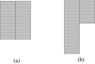
Figure 10: The Fermi energy for a non-interacting Fermi system: in its ground state (a) and in the ground state in an external magnetic field (b). The two boxes represent particles with spin up and down, respectively.

The situation is different at finite $T$. Here the exact Matsubara propagator reads

$$\mathcal{G}_{\alpha\beta}(\vec{k},\omega_{n})=\frac{\delta_{\alpha\beta}}{i\omega_{n}-\left[\epsilon_{\vec{k}}^{(0)}+(-1)^{\alpha+\frac{1}{2}}\mu_{0}B-\mu\right]/\hbar}$$ (46)

and leads to the magnetization

$$\langle\hat{M}\rangle = \frac{\mu_{0}}{\Omega}\int{\d}\vec{x}\int\frac{{\d}\vec{k}}{(2\pi)^{3}}\lim_{\eta\to 0}\frac{1}{\beta\hbar}\sum_{n}e^{i\omega_{n}\eta}$$ (47)

$$\qquad\times\left\{\frac{1}{i\omega_{n}-\left[\epsilon_{\vec{k}}^{(0)}-\mu_{0}B-\mu\right]/\hbar}-\frac{1}{i\omega_{n}-\left[\epsilon_{\vec{k}}^{(0)}+\mu_{0}B-\mu\right]/\hbar}\right\}$$

$$= \mu_{0}\int\frac{{\d}\vec{k}}{(2\pi)^{3}}\left[\frac{1}{e^{\beta(\epsilon_{\vec{k}}^{(0)}-\mu_{0}B-\mu)}+1}-\frac{1}{e^{\beta(\epsilon_{\vec{k}}^{(0)}+\mu_{0}B-\mu)}+1}\right].$$

Clearly, Eq. (47), together with the condition

$$\rho=\frac{\langle\hat{N}\rangle}{\Omega}=\int\frac{{\d}\vec{k}}{(2\pi)^{3}}\left[\frac{1}{e^{\beta(\epsilon_{\vec{k}}^{(0)}-\mu_{0}B-\mu)}+1}+\frac{1}{e^{\beta(\epsilon_{\vec{k}}^{(0)}+\mu_{0}B-\mu)}+1}\right]$$ (48)

fixing the density of the system, in general can be computed only numerically. However, if the magnetic field contributes weakly to the energy eigenvalues, one gets the explicit expression

$$\langle\hat{M}\rangle = -\mu_{0}\int\frac{{\d}\vec{k}}{(2\pi)^{3}}\left[n(\epsilon_{\vec{k}}^{(0)}+\mu_{0}B)-n(\epsilon_{\vec{k}}^{(0)}-\mu_{0}B)\right]$$ (49)

$$\cong -2\mu_{0}^{2}~{}B~{}\int\frac{{\d}\vec{k}}{(2\pi)^{3}}\left.\left(\frac{{\d}n}{{\d}\epsilon_{\vec{k}}}\right)\right|_{\epsilon_{\vec{k}}^{(0)}},$$

which, as it is well-known, in the $T\to 0$ limit, yields the magnetization

$$\langle\hat{M}\rangle=\frac{3\mu_{0}^{2}\rho B}{2\epsilon_{F}}$$ (50)

and the susceptibility

$$\chi\equiv\frac{\partial\langle\hat{M}\rangle}{\partial B}=\frac{3\mu_{0}^{2}\rho}{2\epsilon_{F}},$$ (51)

namely the Pauli paramagnetism. Moreover, in the high temperature limit, the Curie law

$$\chi=\frac{\mu_{0}^{2}\rho}{k_{B}T}$$ (52)

is attained. Thus, Matsubara theory, rather than perturbation theory at $T=0$, yields the correct result.

The above findings relate to the structure of the thermal propagator, which sums over all the possible configurations weighted by the statistical operator and hence leads to the true, symmetry-breaking, ground state in the $T\to 0$ limit.

In fact, by computing the real time Green’s function at finite $T$ through a proper analytical continuation of the thermal propagator and then by taking the vanishing temperature limit, one gets

$$G_{\alpha\beta}(\vec{k},\omega)=\delta_{\alpha\beta}\left[\frac{\theta(\epsilon_{\vec{k}}^{\alpha}-\epsilon_{F})}{\omega-\omega_{k\alpha}+\hbar^{-1}\epsilon_{F}+i\eta}+\frac{\theta(\epsilon_{F}-\epsilon_{\vec{k}}^{\alpha})}{\omega-\omega_{k\alpha}+\hbar^{-1}\epsilon_{F}-i\eta}\right].$$ (53)

By comparing the above with (43), we see that an additional Fermi energy appears in the denominator and, most importantly, $k_{F}$ is replaced by the Fermi energy $\epsilon_{F}$ and $k$ by $\epsilon_{\vec{k}}^{\alpha}$. Thus, the poles in the complex $\omega$-plane of the propagators (53) and (43) (or the associated spectra) are different: hence the contributions they provide to the frequency integral no longer cancel out.

3.2 Dynamic magnetization: the non-interacting linear response theory

In this Subsection we briefly derive the magnetization of the free Fermi gas in the linear response theory at $T=0$. It is well-known that this framework leads to the correct result for the Pauli paramagnetism, since it allows a weak external magnetic field $B(\vec{x},t)$ to break the rotational symmetry of the non-interacting ground state even at $T=0$, thus leading to magnetization.

We start by recalling that turning on a perturbation $\hat{H}^{\mathrm{ext}}$ at time $t=t_{0}$, the fluctuation of the vacuum expectation value of a generic operator $\hat{O}$ at time $t$ reads

$$\delta<\hat{O}(t)> \equiv <\psi_{\mathrm{ext}}(t)|\hat{O}|\psi_{\mathrm{ext}}(t)>-<\psi_{0}|\hat{O}|\psi_{0}>$$ (54)

$$= \frac{i}{\hbar}\int_{t_{0}}^{t}{\d}t^{\prime}<\psi_{0}|\left[\hat{H}_{H}^{\mathrm{ext}}(t^{\prime}),\hat{O}_{H}(t)\right]|\psi_{0}>.$$

In our simple example the perturbation is

$$\hat{H}_{H}^{\mathrm{ext}}(t)=-\mu_{0}\int{\d}\vec{x}\hat{\psi}_{H}^{\dagger}(\vec{x},t)\sigma^{z}\hat{\psi}_{H}(\vec{x},t)B(\vec{x},t)$$ (55)

and the role of $\hat{O}$ is played by

$$\hat{\sigma}_{H}^{z}(\vec{x},t)=\hat{\psi}_{H}^{\dagger}(\vec{x},t)\sigma^{z}\hat{\psi}_{H}(\vec{x},t),$$ (56)

$|\psi_{0}>$ being the Fermi sphere.

Then, the magnetization along the $z$ axis, namely the magnetic moment of the volume element,

$$<\hat{M}_{z}(\vec{x},t)>=\mu_{0}<\hat{\sigma}^{z}(\vec{x},t)>,$$ (57)

is easily expressed as follows

$$\hskip-22.76228pt<\hat{M}_{z}(\vec{x},t)> = \frac{i}{\hbar}\mu_{0}^{2}\int{\d}\vec{x}^{\prime}{\d}t^{\prime}\theta(t-t^{\prime})<\phi_{0}|\left[\hat{\sigma}_{H}^{z}(\vec{x},t),\hat{\sigma}_{H}^{z}(\vec{x}^{\prime},t^{\prime})\right]|\phi_{0}>B(\vec{x}^{\prime},t^{\prime})$$ (58)

$$= -\mu_{0}^{2}\int{\d}\vec{x}^{\prime}{\d}t^{\prime}\Pi^{0R}(\vec{x}t,\vec{x}^{\prime}t^{\prime})B(\vec{x}^{\prime},t^{\prime}),$$

where the retarded spin-spin polarization propagator at zero-order

$$i\hbar\Pi^{0R}_{z,z}(\vec{x}t,\vec{x}^{\prime}t^{\prime})=\theta(t-t^{\prime})<\phi_{0}|\left[\hat{\sigma}_{H}^{z}(\vec{x},t),\hat{\sigma}_{H}^{z}(\vec{x}^{\prime},t^{\prime})\right]|\phi_{0}>$$ (59)

has been introduced. By Fourier-transforming (our system is translationally invariant), Eq. (58) becomes, for $\omega>0$,

$$<\hat{M}_{z}(\vec{k},\omega)>=-\mu_{0}^{2}\Pi^{0}(\vec{k},\omega)B(\vec{k},\omega),$$ (60)

$\Pi^{0}(\vec{k},\omega)$ being the familiar free Fermi gas polarization propagator [6]. The above, in the $\omega\to 0^{+}$ and $k\to 0$ limits, yields the magnetization induced by a static and uniform magnetic field. Since [6]

$$\lim_{k\to 0}\mathrm{Re}\Pi^{0}(\vec{k},0)=-\frac{mk_{F}}{\hbar^{2}\pi^{2}}=-\frac{3}{2}\frac{\rho}{\epsilon_{F}},$$ (61)

one gets

$$<\hat{M}_{z}>=\frac{3}{2}\frac{\rho}{\epsilon_{F}}\mu_{0}^{2}B,$$ (62)

thus recovering the correct susceptibility given by equation (51).

In Eq. (61), the $\omega\to 0$ limit, which implies a static external field, should be taken before the $k\to 0$ one, which implies a uniform external field.

3.3 Static magnetization: the propagator for the interacting Fermi system

We now enlarge the previous analysis by switching on the neutron-neutron interaction

$$V({\vec{x}}_{1}-{\vec{x}}_{2})=\vec{\sigma}_{1}\cdot\vec{\sigma}_{2}V_{1}~{}\frac{\lambda^{2}}{4\pi}\frac{e^{-\lambda|{\vec{x}}_{1}-{\vec{x}}_{2}|}}{|{\vec{x}}_{1}-{\vec{x}}_{2}|}.$$ (63)

The first order self-energy splits now into two pieces that, at finite $T$, read

$$\hskip-5.69046pt\Sigma^{\star++}_{(1)}(\vec{k},T) = -\int\frac{{\d}\vec{k}_{1}}{(2\pi)^{3}}v(\vec{k}-\vec{k}_{1})\left[\frac{1}{e^{\beta(\epsilon^{(0)}_{\vec{k}_{1}}-\mu_{0}B-\mu)}+1}+\frac{2}{e^{\beta(\epsilon^{(0)}_{\vec{k}_{1}}+\mu_{0}B-\mu)}+1}\right]$$ (64a)

$$+V_{1}\int\frac{{\d}\vec{k}_{1}}{(2\pi)^{3}}\left[\frac{1}{e^{\beta(\epsilon^{(0)}_{\vec{k}_{1}}-\mu_{0}B-\mu)}+1}-\frac{1}{e^{\beta(\epsilon^{(0)}_{\vec{k}_{1}}+\mu_{0}B-\mu)}+1}\right]$$

and

$$\hskip-5.69046pt\Sigma^{\star--}_{(1)}(\vec{k},T) = -\int\frac{{\d}\vec{k}_{1}}{(2\pi)^{3}}v(\vec{k}-\vec{k}_{1})\left[\frac{2}{e^{\beta(\epsilon^{(0)}_{\vec{k}_{1}}-\mu_{0}B-\mu)}+1}+\frac{1}{e^{\beta(\epsilon^{(0)}_{\vec{k}_{1}}+\mu_{0}B-\mu)}+1}\right]$$ (64b)

$$-V_{1}\int\frac{{\d}\vec{k}_{1}}{(2\pi)^{3}}\left[\frac{1}{e^{\beta(\epsilon^{(0)}_{\vec{k}_{1}}-\mu_{0}B-\mu)}+1}-\frac{1}{e^{\beta(\epsilon^{(0)}_{\vec{k}_{1}}+\mu_{0}B-\mu)}+1}\right].$$

The associated HF equations then become

$$\left\{\begin{array}[]{rl}\epsilon_{\vec{k}}^{+}&=\epsilon_{\vec{k}}^{(0)}-\mu_{0}B-{\displaystyle\int\frac{{\d}\vec{k}_{1}}{(2\pi)^{3}}v(\vec{k}-\vec{k}_{1})\left(\frac{1}{e^{\beta(\epsilon^{+}_{\vec{k}_{1}}-\mu)}+1}+\frac{2}{e^{\beta(\epsilon^{-}_{\vec{k}_{1}}-\mu)}+1}\right)}\\ &\quad+V_{1}{\displaystyle\int\frac{{\d}\vec{k}_{1}}{(2\pi)^{3}}\left(\frac{1}{e^{\beta(\epsilon^{+}_{\vec{k}_{1}}-\mu)}+1}-\frac{1}{e^{\beta(\epsilon^{-}_{\vec{k}_{1}}-\mu)}+1}\right)}\\ \epsilon_{\vec{k}}^{-}&=\epsilon_{\vec{k}}^{(0)}+\mu_{0}B-{\displaystyle\int\frac{{\d}\vec{k}_{1}}{(2\pi)^{3}}v(\vec{k}-\vec{k}_{1})\left(\frac{2}{e^{\beta(\epsilon^{+}_{\vec{k}_{1}}-\mu)}+1}+\frac{1}{e^{\beta(\epsilon^{-}_{\vec{k}_{1}}-\mu)}+1}\right)}\\ &\quad-V_{1}{\displaystyle\int\frac{{\d}\vec{k}_{1}}{(2\pi)^{3}}\left(\frac{1}{e^{\beta(\epsilon^{+}_{\vec{k}_{1}}-\mu)}+1}-\frac{1}{e^{\beta(\epsilon^{-}_{\vec{k}_{1}}-\mu)}+1}\right)}\\ \rho&={\displaystyle\int\frac{{\d}\vec{k}_{1}}{(2\pi)^{3}}\left(\frac{1}{e^{\beta(\epsilon^{+}_{\vec{k}_{1}}-\mu)}+1}+\frac{1}{e^{\beta(\epsilon^{-}_{\vec{k}_{1}}-\mu)}+1}\right)}.\end{array}\right.$$ (65)

From Eqs. (64) and (65) it appears that, owing to the presence of the magnetic field $B$, the self-energy not only is no longer proportional to the unit matrix in spin space, but it acquires, beyond the exchange contribution, a direct one as well, an occurrence with far reaching consequences.

We have solved the system (65) numerically, searching for the magnetization in Eq. (47) and the HF chemical potential $\mu_{\mathrm{HF}}$. Our results for $\mu_{\mathrm{HF}}$ are displayed in Figs. 12 and 12. For purpose of illustration we have chosen the very large value of $10^{14}$ tesla for $B$ (on the surface of neutron stars $B$ is estimated to range from $10^{8}$ to $10^{10}$ tesla [7], whereas in the interior its upper limit is set at a few times $10^{14}$ tesla [8]).

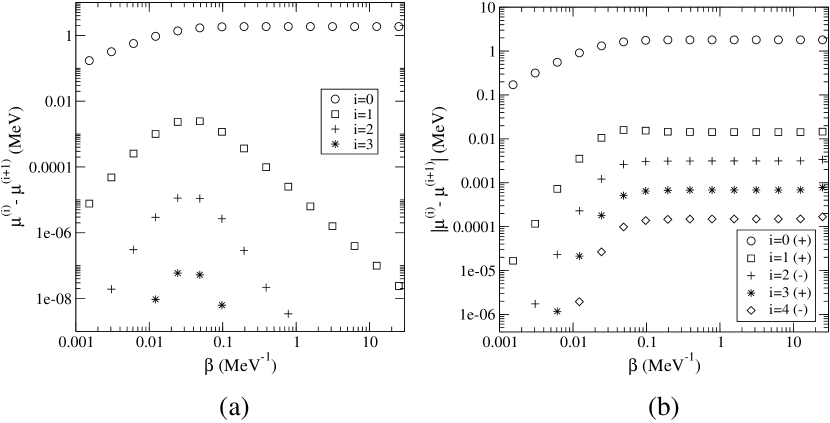
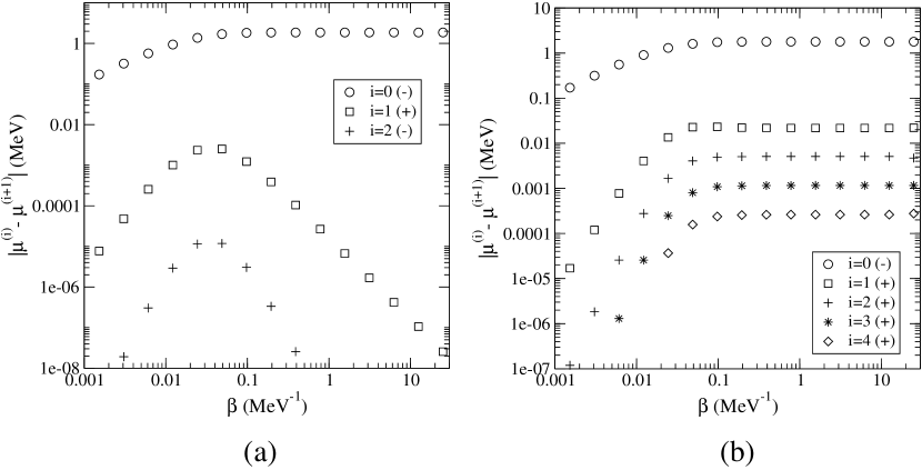
Figure 11: The difference between the successive HF iterations $\mu^{(i)}-\mu^{(i+1)}$ as a function of $\beta$ in the case of a finite range interaction with $\lambda=140$ MeV and $V_{1}=50$ MeV fm³ in absence of magnetic field (a) and with a background magnetic field $B=10^{14}$ tesla (b); $\rho=0.17$ fm^-3. In panel (b) the modulus of the differences is displayed: note the alternation in sign that implies an oscillating approach to $\mu_{\mathrm{HF}}$.

Figure 12: As in Fig. 12, but with $V_{1}=-50$ MeV fm³. Note that the differences are now constant in sign, except the first one: hence the approach to $\mu_{\mathrm{HF}}$ is smooth.

Remarkably, in the presence of a magnetic field the contributions to $\mu_{\mathrm{HF}}$ arising from the higher iterations (Fig. 12b) are seen to stay quite constant with the temperature till very small $T$, unlike the case with no symmetry breaking (Fig. 12a), where they reach a maximum for temperatures close to $T_{F}$.

In the proximity of $T=0$, the higher order diagrams contributing to $\mu_{\mathrm{HF}}$, rather than canceling each other, now contribute more than they do at high $T$. This is a beautiful manifestation of the failure of the cancellation theorem in the presence of a symmetry breaking.

Of significance is also the alternating behavior of the iterations for an antiferromagnetic interaction: those of odd order have a positive sign, those of even order a negative sign (note that in Fig. 12b we display the absolute value of $\mu^{(i)}-\mu^{(i+1)}$). As a consequence the approach to the HF self-consistent solution is no longer smooth, as in the symmetric case, but now the successive iterations oscillate around the HF solution until they stabilize at the latter value when self-consistency is reached.

In contrast, it is remarkable that for the ferromagnetic coupling the sign of the successive iterations is constant (positive), except for the first one, which is negative. Hence, in this case the self-consistent solution is smoothly reached. The situation is reminiscent of the physics of an hydrogen atom in an external magnetic field, the competition between the Coulomb and the magnetic field now being replaced by the one between the nucleon-nucleon interaction and the magnetic field. If this opposes the action of the nucleon-nucleon forces, then it makes it harder to reach self-consistency.

3.4 Dynamic magnetization: the interacting linear response theory

As previously seen for the case of a non-interacting Fermi system, also when the interaction is switched on we can obtain the system’s magnetization and susceptibility in the framework of the linear response theory at $T=0$ using the polarization propagator, a tool set up with the two-fermion Green’s function.

We start by computing the spin-spin retarded polarization propagator needed in the HF theory. In the present case, owing to the nature of the interaction in Eq. (63), only the Fock term is non-vanishing, so we shall actually compute $\Pi^{\mathrm{F}}$. At $T=0$ its real part reads

$$\mathrm{Re}\Pi^{\mathrm{F}}(\vec{q},\omega)=\frac{2}{\hbar}\mathcal{P}\int\frac{{\d}\vec{k}}{(2\pi)^{3}}\theta(\mid\vec{k}+\vec{q}\mid-k_{F})]\theta(k_{F}-k)\frac{2\omega_{\vec{k}\vec{q}}}{\omega^{2}-(\omega_{\vec{k}\vec{q}})^{2}},$$ (66)

where

$$\omega_{\vec{k}\vec{q}}=\omega_{\vec{k}+\vec{q}}+\Sigma^{\star}_{(1)}(\vec{k}+\vec{q})-\omega_{\vec{k}}-\Sigma^{\star}_{(1)}(\vec{k}).$$ (67)

The above expression cannot be computed analytically. Yet, in the case of the interaction in Eq. (63), a quite accurate analytic approximation to Eq. (66) can be obtained by expanding the self-energy in Eq. (31) (divided by 3, since we dropped the isospin degree of freedom) up to and including terms in $k^{2}$; one gets

$$\Sigma^{\star}_{(1)}(\vec{k})=A+Bk^{2},$$ (68)

with

$$A=\frac{3\lambda^{3}V_{1}}{2\hbar\pi^{2}}\left(\arctan\frac{k_{F}}{\lambda}-\frac{k_{F}}{\lambda}\right)$$ (69)

and

$$B=\frac{k_{F}^{3}\lambda^{2}V_{1}}{2\hbar\pi^{2}(k_{F}^{2}+\lambda^{2})^{2}}.$$ (70)

Then, computing $\Sigma^{\star}(\vec{k}+\vec{q})-\Sigma^{\star}(\vec{k})$ in this approximation and inserting this result into Eq. (66), we get for $\mathrm{Re}\Pi^{\mathrm{F}}$ an expression identical to the free one, but for the replacement of the nucleon mass $m$ with an effective mass $m^{\star}$ given by

$$\frac{m^{\star}}{m}=\left[1+\frac{k_{F}^{3}\lambda^{2}mV_{1}}{\hbar^{2}\pi^{2}(k_{F}^{2}+\lambda^{2})^{2}}\right]^{-1}.$$ (71)

Next, letting as before first $\omega\to 0$ and then $q\to 0$, we obtain for the magnetization and the magnetic susceptibility the expressions

$$<\hat{M}_{z}>=\frac{3}{2}\frac{\rho}{\epsilon_{F}^{\star}}\mu_{0}^{2}B$$ (72a)

and

$$\chi=\frac{3}{2}\frac{\rho}{\epsilon_{F}^{\star}}\mu_{0}^{2},$$ (72b)

respectively, where the Fermi energy now reads $\epsilon_{F}^{\star}=\hbar^{2}k_{F}^{2}/2m^{\star}$. Since, for the interaction in Eq. (63) with $V_{1}>0$, one has $m^{\star}<m$, we conclude that for an antiferromagnetic force the HF mean field lowers the free magnetization (or the susceptibility).

However it is of significance that Eq. (72a) does not coincide with the $T\to 0$ limit of the magnetization

$$\langle\hat{M}\rangle=\mu_{0}\int\frac{{\d}\vec{k}}{(2\pi)^{3}}\left[\frac{1}{e^{\beta(\epsilon^{+}_{\vec{k}}-\mu)}+1}-\frac{1}{e^{\beta(\epsilon^{-}_{\vec{k}}-\mu)}+1}\right],$$ (73)

$\epsilon^{+}_{\vec{k}}$, $\epsilon^{-}_{\vec{k}}$ and $\mu$ being the HF single-particle energies and chemical potential obtained by solving Eq. (65). To achieve the accord between Eqs. (72a) and (73) it is necessary to go beyond HF. This will be done in the next Section.

Here we display in Fig. 13 the temperature behavior of the relative magnetization $M$ (yielding the fraction of spins anti-aligned to the magnetic field, i.e. $M=<\hat{M}_{z}>/|\mu_{0}|\rho=(N^{\uparrow}-N^{\downarrow})/(N^{\uparrow}+N^{\downarrow})$ with obvious meaning of the symbols) associated with Eq. (73). Note the decreasing of $M$ as $T$ increases and the recovery at large $T$ of the Curie value, the interaction among neutrons becoming irrelevant at high $T$. Moreover the values of $M$ at $T=0$ are lower (larger) than the free one for an antiferromagnetic (ferromagnetic) force: they will be shown to coincide with the predictions of the linear response theory in a frame extending the HF one.

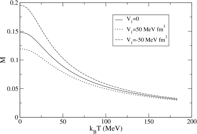
Figure 13: The HF magnetization in an external magnetic field as a function of temperature for $B=10^{14}$ tesla and for different values of $V_{1}$; $\lambda=140$ MeV and $\rho=0.17$ fm^-3.

4 Beyond HF

In the framework of the linear response theory the natural extension of the HF approach should embody the RPA (random phase approximation) correlations. To start with, we neglect the exchange terms, i.e. we make use of the simpler ring approximation.

This yields for the spin-spin polarization propagator of a homogeneous infinite system the expression

$$\Pi^{\mathrm{ring}}(\vec{q},\omega)=\frac{\Pi^{\mathrm{F}}(\vec{q},\omega)}{1-V_{1}\frac{\displaystyle\lambda^{2}}{\displaystyle q^{2}+\lambda^{2}}\Pi^{\mathrm{F}}(\vec{q},\omega)},$$ (74)

from where the magnetization

$$<\hat{M}>=-\lim_{q\to 0}\lim_{\omega\to 0}\mathrm{Re}\Pi^{\mathrm{ring}}(\vec{q},\omega)\mu_{0}^{2}B=\frac{3\rho/2\epsilon_{F}^{\star}}{1+V_{1}(3\rho/2\epsilon_{F}^{\star})}\mu_{0}^{2}B,$$ (75)

which is linear in $B$, is deduced. Thus, for the magnetic susceptibility in ring approximation, one gets

$$\chi^{\mathrm{ring}}=\frac{3\rho/2\epsilon_{F}^{\star}}{1+V_{1}(3\rho/2\epsilon_{F}^{\star})}\mu_{0}^{2},$$ (76)

showing that the ring correlations, for an anti-ferromagnetic $(V_{1}>0)$ nucleon-nucleon interaction, lower the susceptibility of the free Fermi gas, thus acting in the same direction of the HF mean field.

The quenching of the free Fermi gas susceptibility $\chi^{\mathrm{free}}$ in ring approximation relates to the existence of a spin collective mode, called a magnon, which makes harder the excitation of the system. As it is well-known, the energy of the magnon is found by solving the equation

$$1-V_{1}\frac{\lambda^{2}}{q^{2}+\lambda^{2}}\mathrm{Re}\Pi^{\mathrm{F}}(\vec{q},\omega)=0,$$ (77)

that — in the limit $\omega\to 0$, $q\to 0$, but keeping now the ratio $x=(\omega/q)m^{\star}/\hbar k_{F}$ constant and greater than one — is fulfilled by the phonon-like dispersion relation $\omega=c_{S}q$, the zero-sound velocity $c_{S}$ being fixed by the equation [6]

$$\Phi(x)=\frac{\pi^{2}\hbar^{2}}{m^{\star}k_{F}V(0)},$$ (78)

with

$$\Phi(x)=\frac{1}{2}x\ln\frac{x+1}{x-1}-1.$$ (79)

To assess the role of anti-symmetrization one resorts to the full RPA, which includes the exchange diagrams beyond the ring ones. This we do with the method of the continued fractions [9, 10, 11], which, when truncated at the first fraction, yields for the RPA polarization propagator the following expression

$$\Pi^{\mathrm{RPA}}(\vec{q},\omega)=\frac{\Pi^{\mathrm{F}}(\vec{q},\omega)}{1-V_{1}\frac{\displaystyle\lambda^{2}}{\displaystyle q^{2}+\lambda^{2}}\Pi^{\mathrm{F}}(\vec{q},\omega)-\Pi^{\mathrm{F}(1)}_{\text{ex}}(\vec{q},\omega)/\Pi^{\mathrm{F}}(\vec{q},\omega)},$$ (80)

where

$$\Pi^{\mathrm{F}(1)}_{\text{ex}}(\vec{q},\omega)=-\int\frac{{\d}\vec{k}_{1}}{(2\pi)^{3}}E(\vec{k}_{1},\vec{q})\int\frac{{\d}\vec{k}_{2}}{(2\pi)^{3}}E(\vec{k}_{2},\vec{q})v(\vec{k}_{1}-\vec{k}_{2}),$$ (81)

being

$$E(\vec{k},\vec{q})=\frac{1}{\hbar}\left[\frac{\theta(|\vec{k}+\vec{q}|-k_{F})\theta(k_{F}-k)}{\omega-\omega_{\vec{k}+\vec{q}}+\omega_{\vec{k}}+i\eta}-\frac{\theta(k_{F}-|\vec{k}+\vec{q}|)\theta(k-k_{F})}{\omega-\omega_{\vec{k}+\vec{q}}+\omega_{\vec{k}}-i\eta}\right],$$ (82)

is the exchange diagram associated to the first order ring contribution. The expression in Eq. (80), while exact for a zero-range force, remains a good approximation for typical nuclear finite range interactions too.

One can verify that the magnetization deduced from Eq. (80) embodies a susceptibility very close to the exact RPA one, since the RPA problem can be analytically solved for an infinite system in the limit of vanishing frequencies and momenta, where it merges with the Landau’s quasi-particle theory [12, 13]. One gets (see Appendix B)

$$\chi^{\mathrm{RPA}}=\frac{3\rho/2\epsilon_{F}^{\star}}{1+V_{1}(3\rho/2\epsilon_{F}^{\star})+{\textstyle\frac{1}{2}}V_{1}(3\rho/2\epsilon_{F}^{\star})(\lambda/2k_{F})^{2}\ln\left[1+(2k_{F}/\lambda)^{2}\right]}\mu_{0}^{2},$$ (83)

which, for a zero-range force, becomes

$$\chi^{\mathrm{RPA}}_{\mathrm{0-range}}=\frac{3\rho/2\epsilon_{F}}{1+9V_{1}\rho/4\epsilon_{F}},$$ (84)

an expression identical to the one deduced from (80). Eq. (83) shows that, in the anti-ferromagnetic case, the anti-symmetrization reinforces (mildly) the quenching of $\chi^{\mathrm{free}}$ induced by the ring correlations.

Note that in RPA the impact of the exchange diagrams decreases as the range of the force increases, as it should: this result follows by comparing Eq. (83) with Eq. (84).

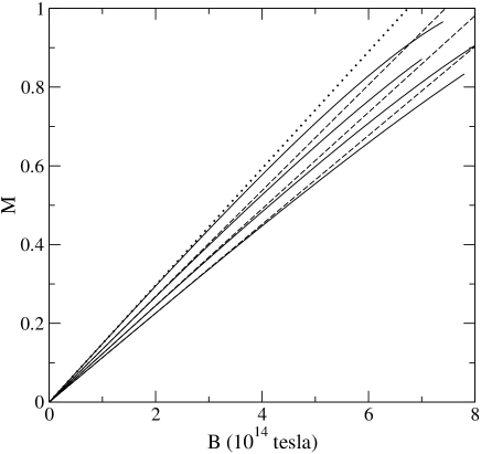
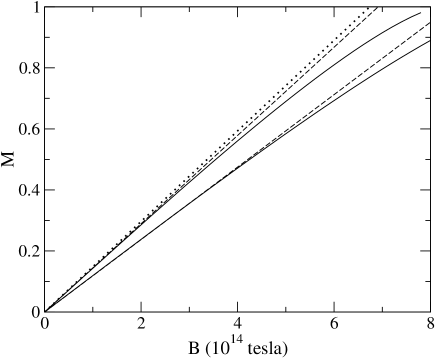
Figure 14: The magnetization as a function of $B$ for $V_{1}=50$ MeV fm³ and zero range at $T=0$ ($\rho=0.17$ fm^-3). The dotted lines display the results in the linear response framework (using $\Pi$), the solid lines in the thermal self-consistent calculations at $T=0$ (using $\mathcal{G}^{B}$). Starting from above the pairs of curves correspond, respectively, to the following cases: $\Pi^{0}$/$\mathcal{G}_{0}^{B}$, $\Pi^{\text{ladder}}$/$\mathcal{G}_{\text{F}}^{B}$, $\Pi^{\text{ring}}$/$\mathcal{G}_{\text{H}}^{B}$, $\Pi^{\text{RPA}}$/$\mathcal{G}_{\text{HF}}^{B}$.

Figure 15: The magnetization as a function of $B$ for $V_{1}=50$ MeV fm³ and $\lambda=140$ MeV at $T=0$ ($\rho=0.17$ fm^-3). The dotted line displays the result in the free linear response framework ($\Pi^{0}$), the upper dashed line in the linear response framework with Fock correlations ($\Pi_{\text{F}}$) and the lower dashed line with Fock and RPA correlations ($\Pi_{\text{F}}^{\text{RPA}}$); the upper solid line represents the results of the thermal self-consistent calculations at $T=0$ including only Fock correlations ($\mathcal{G}_{\text{F}}^{B}$), the lower solid line includes HF correlations ($\mathcal{G}_{\text{HF}}^{B}$).

We are now in a position to find out the polarization propagator yielding (as long as the response of the system is linear) the HF Matsubara magnetization. For the sake of simplicity we start by considering a zero-range antiferromagnetic force of strength $V_{1}=50$ MeV. In Figs. 15 and 15 are displayed versus $B$ various relative magnetizations as obtained from the Matsubara propagator and from the zero-temperature linear response theory. In Fig. 15 we employ a zero-range force, hence the HF mean field does not contribute to the polarization propagators; in Fig. 15 a finite range force. The figures clearly show that the magnetization obtained from $\Pi^{RPA}$ coincides with the one given by the HF thermal propagator $\mathcal{G}_{HF}^{B}$ for $T\to 0$ until $\bar{B}\simeq 3$ (in units of $10^{14}$ tesla), which sets the limit of validity of the linear response framework. For $B$ larger than $\bar{B}$ the magnetization increases much less rapidly than linearly until it saturates when the system is fully magnetized, an expected behavior correctly reproduced by the thermal HF theory. We thus conclude that in order to obtain the magnetization and, in general, any mean value using the single-particle thermal propagator $\mathcal{G}_{HF}^{B}$, it is necessary to sum up an infinite series of loop diagrams in the particle-hole polarization propagator, namely those of RPA. This correspondence extends also to the pure ring and ladder polarization propagator as illustrated in Table 1 (with $\Pi^{\text{ladder}}$ we mean the propagator summing up only the particle-hole exchange diagram).

Susceptibility	Feynman, $T=0$	Matsubara, $T\to 0$
$\chi^{\text{free}}$	$\Pi^{0}$	$\mathcal{G}_{0}^{B}$
$\chi^{\text{ring}}$	$\Pi^{\text{ring}}$	$\mathcal{G}_{\text{H}}^{B}$
$\chi^{\text{ladder}}$	$\Pi^{\text{ladder}}$	$\mathcal{G}_{\text{F}}^{B}$
$\chi^{\text{RPA}}$	$\Pi^{\text{RPA}}$	$\mathcal{G}_{\text{HF}}^{B}$

Table 1: The zero-temperature polarization propagator required to obtain the same magnetic susceptibility deduced (in the $T\to 0$ limit) from the Matsubara free ($\mathcal{G}_{0}^{B}$), Hartree ($\mathcal{G}_{\text{H}}^{B}$), Fock ($\mathcal{G}_{\text{F}}^{B}$) and HF ($\mathcal{G}_{\text{HF}}^{B}$) thermal single-particle propagator. Clearly the many body diagrams summed up to infinite order to get the appropriate $\Pi$ are the ring, the ladder and the RPA ones, respectively.

Also worth noticing is that the range of validity of the linear response theory appears to be only moderately affected by the many body scheme employed.

Turning now to comment on the finite range force, we observe that the slopes of the curves in Fig. (15) are somewhat reduced with respect to those in Fig. (15). Indeed, in the former the fermionic lines in the polarization propagator are dressed by a $k^{2}$ dependent Fock self-energy and this, as previously shown, reduces the susceptibility for an antiferromagnetic interaction. Furthermore, as expected, $\Pi_{\text{F}}^{\text{ring}}$ and $\Pi_{\text{F}}^{\text{RPA}}$ tend to become very similar as the range of the force increases.

Thus we have reached the result that the statistical average required in computing $\mathcal{G}_{\text{HF}}^{B}$ is performed over the states entering into the spectral representation of the RPA polarization propagator with fermionic lines dressed by a Fock self-energy.

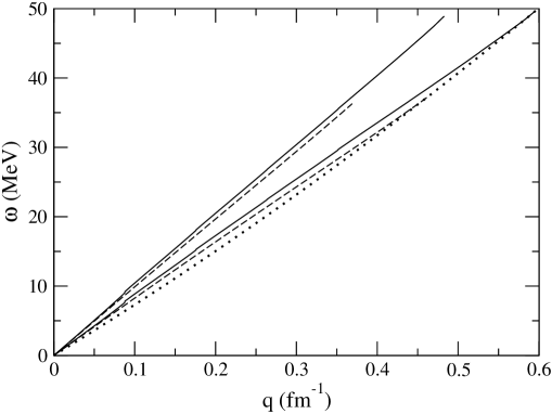
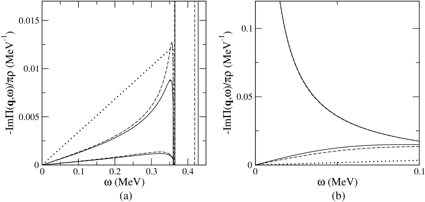
Figure 16: The dispersion relation for the collective modes (magnons) in ring (dashed) and RPA (solid), with (upper lines) and without (lower lines) the HF mean field for an antiferromagnetic interaction with $V_{1}=480$ MeV fm³ and $\lambda=140$ MeV ($\rho=0.17$ fm^-3); the dotted line represents the upper border of the ph response region, $q^{2}/2m+qk_{F}/m$.

Figure 17: Spin response functions at $q=1$ MeV/c, $\rho=0.17$ fm^-3 and for a finite range interaction with $\lambda=140$ MeV. The dotted lines represent the free response, the dashed and solid lines the ring and RPA ones, respectively. In panel (a) we employ antiferromagnetic couplings: $V_{1}=150$ MeV fm³ (upper curves) and $V_{1}=480$ MeV fm³ lower curves; the spikes represent the ring and RPA collective states: the pair at higher energy corresponds to $V_{1}=480$ MeV fm³, the other one to $V_{1}=150$ MeV fm³ (note that in the latter case the ring and RPA excitations energies are very close). In panel (b) we employ ferromagnetic couplings: $V_{1}=-150$ MeV fm³ (lower curves), $V_{1}=V_{1,\text{crit}}^{\text{ring}}\cong-239$ MeV fm³ and $V_{1}=V_{1,\text{crit}}^{\text{RPA}}\cong-223$ MeV fm³ (note that the ring response at $V_{1}=V_{1,\text{crit}}^{\text{ring}}$ and the RPA one at $V_{1}=V_{1,\text{crit}}^{\text{RPA}}$ practically overlap each other). For the sake of simplicity, the HF mean field has not been included.

In concluding this Section we display in Fig. 17 the frequency behavior of the magnons, both in ring and in RPA, with and without the HF mean field, for an interaction with $V_{1}=480$ MeV fm³ and $\lambda=140$ MeV. The hardening of the magnon mode stemming from the HF mean field and (to less extent) from anti-symmetrizing the ring diagrams is clearly apparent in the figure.

We display also in Fig. 17 the system’s spin response functions (proportional to the imaginary part of $\Pi(\vec{q},\omega)$) both in ring and in RPA and both for an antiferromagnetic and a ferromagnetic coupling at $q=1$ MeV/c. For sake of illustrating the impact of the pure ring and RPA correlations on the response we ignore in the figure the action of the Fock mean field (namely, we compute Eqs. (74) and (80) replacing $\Pi^{\text{F}}$ with $\Pi^{0}$, or, in other words, we set $m^{*}=m$). The values chosen for the coupling are $V_{1}=\pm 150,480,-239$ and $-223$ MeV fm³, whereas the range parameter is $\lambda=140$ MeV. In the figure it is clearly seen that:

• for an anti-ferromagnetic coupling, as expected, the magnons are standing out above the particle-hole (ph) continuum, the more so the larger $V_{1}$ is. Correspondingly, the depletion of the ph continuum increases with $V_{1}$. Note also that the impact of anti-symmetrization is modest, as expected owing to the long range of the force: the more so, the larger $V_{1}$ is;

• for the ferromagnetic coupling the response is of course enhanced, the enhancement becoming however dramatic for $V_{1}=-239$ MeV fm³ in ring and for $V_{1}=-223$ MeV fm³ in RPA. These values of the coupling are those yielding a divergent ring and RPA susceptibility, respectively, when $m^{*}=m$. We shall return on this point in the next Section.

5 The spontaneous symmetry breaking

From the explicit formulas of $\chi^{\mathrm{ring}}$ and $\chi^{\mathrm{RPA}}$ obtained in the linear response scheme one sees that both susceptibilities diverge in the case of a ferromagnetic coupling in correspondence to the following critical values of the strength of the force:

$$V_{1,\mathrm{crit}}^{\mathrm{ring}}=-\frac{2\epsilon^{*}_{F}}{3\rho}\Rightarrow V_{1,\mathrm{crit}}^{\mathrm{ring}}=-\frac{\pi^{2}\hbar^{2}}{mk_{F}}\frac{(1+\bar{\lambda}^{2})^{2}}{\bar{\lambda}^{4}+3\bar{\lambda}^{2}+1}$$ (85a)

and

$$V_{1,\mathrm{crit}}^{\mathrm{RPA}} = -\frac{2\epsilon^{*}_{F}}{3\rho}\frac{1}{1+{\textstyle\frac{1}{2}}(\lambda/2k_{F})^{2}\ln\left[1+(2k_{F}/\lambda)^{2}\right]}\Rightarrow$$

$$V_{1,\mathrm{crit}}^{\mathrm{RPA}} = -\frac{\pi^{2}\hbar^{2}}{mk_{F}}\frac{(1+\bar{\lambda}^{2})^{2}}{\bar{\lambda}^{4}+3\bar{\lambda}^{2}+1+\frac{1}{2}(1+\bar{\lambda}^{2})^{2}(\bar{\lambda}/2)^{2}\ln[1+(2/\bar{\lambda})^{2}]}$$ (85b)

with $\bar{\lambda}=\lambda/k_{F}$. The above expressions have been deduced making use of Eq. (71), which yields the neutron effective mass $m^{*}$ in terms of $V_{1}$, $\lambda$ and $k_{F}$.

The behavior of Eqs. (85a) and (85) versus $\bar{\lambda}=\lambda/k_{F}$ is displayed in Fig. 18: note that the two curves coincide for an infinite range force ($\bar{\lambda}=0$) whereas their difference is the largest for a contact interaction ($\bar{\lambda}=\infty$). For $\lambda=140$ MeV and $k_{F}=1.71$ fm^-1 one has $V_{1,\mathrm{crit}}^{\mathrm{ring}}\cong-239$ MeV fm³ and $V_{1,\mathrm{crit}}^{\mathrm{RPA}}\cong-223$ MeV fm³: these are the values previously employed (see Fig. 17).

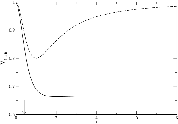
Figure 18: The behavior of the critical interactions $V_{1,\mathrm{crit}}^{\mathrm{ring}}$ (dashed) and $V_{1,\mathrm{crit}}^{\mathrm{RPA}}$ (solid) versus $\bar{\lambda}=\lambda/k_{F}$ in units of $-\pi^{2}\hbar^{2}/mk_{F}$. The arrow corresponds to $\lambda=140$ MeV and $k_{F}=1.71$ fm^-1.

In this Section, for sake of simplicity, we shall consider a zero-range force ($\lambda=\infty$). In this instance, always with $k_{F}=1.71$ fm^-1, which corresponds to a neutron density $\rho=0.17$ fm^-3, one gets $V_{1,\mathrm{crit}}^{\mathrm{ring}}\cong-239$ MeV fm³ and $V_{1,\mathrm{crit}}^{\mathrm{RPA}}\cong-159$ MeV fm³, respectively. We remark that the value of $V_{1}^{\mathrm{ring}}$ for a zero range force coincides with the one of Ref. [3], which in turn is identical to what one gets in the Hartree theory, as we shall later see.

The values of the couplings in Eq. (85) signal the occurrence of a spontaneous symmetry breaking: correspondingly, a phase transition takes place in the system from a phase fully symmetric to a phase where the rotational invariance is broken in spin space. Hence, the vacuum appropriate to this new phase should be characterized by two Fermi momenta $k_{F}^{+}$ and $k_{F}^{-}$, associated with neutrons with spin up and down, respectively.

In this situation the free Fermi propagator, while still diagonal in spin space, is no longer proportional to the unit matrix, but becomes

$$G^{0,\mathrm{b}}(\vec{k},\omega)=\left(\begin{array}[]{cc}G^{0,\mathrm{b}}_{++}(\vec{k},\omega)&0\\ 0&G^{0,\mathrm{b}}_{--}(\vec{k},\omega)\end{array}\right),$$ (86)

where

$$G^{0,\mathrm{b}}_{++}(\vec{k},\omega) = \frac{\theta(k-k_{F}^{+})}{\omega-\omega_{\vec{k}}+i\eta}+\frac{\theta(k_{F}^{+}-k)}{\omega-\omega_{\vec{k}}-i\eta},$$ (87a)

$$G^{0,\mathrm{b}}_{--}(\vec{k},\omega) = \frac{\theta(k-k_{F}^{-})}{\omega-\omega_{\vec{k}}+i\eta}+\frac{\theta(k_{F}^{-}-k)}{\omega-\omega_{\vec{k}}-i\eta}$$ (87b)

and $\omega_{\vec{k}}=\hbar k^{2}/2m=\epsilon^{(0)}_{\vec{k}}$.

With the above propagator the first order momentum independent self-energy is easily computed and, as expected, splits into two terms, namely

$$\hbar\Sigma_{++} = \frac{V_{1}}{6\pi^{2}}\left[\left({k_{F}^{+}}^{3}-{k_{F}^{-}}^{3}\right)-\left({k_{F}^{+}}^{3}+2{k_{F}^{-}}^{3}\right)\right]$$ (88a)

$$\hbar\Sigma_{--} = \frac{V_{1}}{6\pi^{2}}\left[\left({k_{F}^{-}}^{3}-{k_{F}^{+}}^{3}\right)-\left({k_{F}^{-}}^{3}+2{k_{F}^{+}}^{3}\right)\right]$$ (88b)

of obvious physical meaning.

In Eq. (88) both the direct (first term on the right hand side) and the exchange (second term) contributions are neatly separated out. Note that the direct term is the same in both $\Sigma_{++}$ and $\Sigma_{--}$, but for the sign, and moreover it vanishes, as it should, for $k_{F}^{+}=k_{F}^{-}$.

Since for a homogeneous infinite system the HF problem is trivial at $T=0$, even in a broken vacuum, then the exact HF fermion propagator is easily obtained by replacing Eq. (87) with

$$\hskip-22.76228ptG^{\mathrm{HF},\mathrm{b}}_{++}(\vec{k},\omega) = \frac{\theta(k-k_{F}^{+})}{\omega-(\omega_{\vec{k}}-3V_{1}{k_{F}^{-}}^{3}/6\pi^{2}\hbar)+i\eta}+\frac{\theta(k_{F}^{+}-k)}{\omega-(\omega_{\vec{k}}-3V_{1}{k_{F}^{-}}^{3}/6\pi^{2}\hbar)-i\eta},$$

$$\hskip-22.76228ptG^{\mathrm{HF},\mathrm{b}}_{--}(\vec{k},\omega) = \frac{\theta(k-k_{F}^{-})}{\omega-(\omega_{\vec{k}}-3V_{1}{k_{F}^{+}}^{3}/6\pi^{2}\hbar)+i\eta}+\frac{\theta(k_{F}^{-}-k)}{\omega-(\omega_{\vec{k}}-3V_{1}{k_{F}^{+}}^{3}/6\pi^{2}\hbar)-i\eta}.$$

The above, to be viewed as a generalized HF fermion propagator in a vacuum not invariant for spin rotations, embodies the HF single-particle energies

$$\epsilon_{\vec{k}}^{\pm}=\epsilon_{\vec{k}}^{(0)}-\frac{3V_{1}}{6\pi^{2}}{k_{F}^{\mp}}^{3}=\epsilon_{\vec{k}}^{(0)}-\frac{3}{2}V_{1}\rho(1\mp M)$$ (90)

and allows to compute the HF energy per particle in terms of the relative magnetization $M=(N^{\uparrow}-N^{\downarrow})/(N^{\uparrow}+N^{\downarrow})$ and of the density $\rho=(N^{\uparrow}+N^{\downarrow})/\Omega$ according to

$$\frac{E}{N} = \frac{1}{\rho}\int\frac{{\d}\vec{k}}{(2\pi)^{3}}\left[\epsilon_{\vec{k}}^{(0)}-\frac{3}{2}V_{1}\frac{{k_{F}^{-}}3}{6\pi^{2}}\right]\theta(k_{F}^{+}-k)$$ (91)

$$\quad+\frac{1}{\rho}\int\frac{{\d}\vec{k}}{(2\pi)^{3}}\left[\epsilon_{\vec{k}}^{(0)}-\frac{3}{2}V_{1}\frac{{k_{F}^{+}}3}{6\pi^{2}}\right]\theta(k_{F}^{-}-k)$$

$$= \frac{3}{10}\epsilon_{F}^{(0)}\left[(1+M)^{5/3}+(1-M)^{5/3}\right]-\frac{3}{4}V_{1}\rho(1-M^{2}).$$

Here $N^{\uparrow}/\Omega={k_{F}^{+}}^{3}/6\pi^{2}$ and $N^{\downarrow}/\Omega={k_{F}^{-}}^{3}/6\pi^{2}$ correspond to the spin up and spin down densities, respectively. Likewise, one can easily write down the expressions for $\epsilon^{\pm}_{\vec{k}}$ and $E/N$ in Hartree and in Fock approximation separately. We remark that Eq. (90) coincides with the single-particle energies obtained by solving Eq. (65), with a zero-range force, in the limit $T\to 0$, $B\to 0$.

Now, for the system to be in equilibrium the two chemical potentials (Fermi energies at $T=0$) of the spin up and spin down fermions should be equal. Hence, in HF the equation

$$\frac{\hbar^{2}{k_{F}^{+}}^{2}}{2m}-\frac{3V_{1}}{6\pi^{2}}{k_{F}^{-}}^{3}=\frac{\hbar^{2}{k_{F}^{-}}^{2}}{2m}-\frac{3V_{1}}{6\pi^{2}}{k_{F}^{+}}^{3}$$ (92)

should be fulfilled and similar equations should hold in the Hartree and in the Fock approximation as well. Notably all the three cases can be compactified into the single equation

$$(1+M)^{2/3}-(1-M)^{2/3}=-\alpha\frac{V_{1}\rho}{\epsilon_{F}{(0)}}M,$$ (93)

with

$$\begin{array}[]{ll}\alpha=3&\mathrm{in~{}HF}\\ \alpha=2&\mathrm{in~{}Hartree}\\ \alpha=1&\mathrm{in~{}Fock}.\end{array}$$ (94)

In the context of solid state physics Eq. (93) is usually referred to as Stoner equation. Of course, the values in Eq. (94) for $\alpha$ are valid only for a zero-range force.

It is a remarkable occurrence that one arrives exactly at the same Eq. (93) by minimizing the energy per particle in Eq. (91) with respect to the magnetization. This outcome is a consequence of the Hugenholtz-Van Hove theorem [14], which remains true even in a broken vacuum.

Now, the Stoner equation in Eq. (93) admits real solutions only for $M$ in the range $0\leq M\leq 1$. For a given density $\rho$, which also fixes $\epsilon_{F}^{(0)}$, the case $M=1$, corresponding to a fully magnetized system, leads to the critical value for the coupling

$$V_{1,\mathrm{crit}}^{\mathrm{upper}}=-\frac{2^{2/3}}{\alpha}\frac{\epsilon_{F}^{(0)}}{\rho}.$$ (95)

This expression cannot be derived in the linear response framework and with $\alpha=2$ (Hartree approximation) is identical to the mean field value quoted in Ref. [3].

Instead, in the case $M=0^{+}$ (incipient ferromagnetism) Eq. (93) leads to

$$V_{1,\mathrm{crit}}^{\mathrm{lower}}=-\frac{4}{3\alpha}\frac{\epsilon_{F}^{(0)}}{\rho}.$$ (96)

This result, when $\alpha=2$ (Hartree approximation), coincides with the linear response value in ring approximation in Eq. (85a), whereas, when $\alpha=3$ (HF approximation), coincides with the linear response value in RPA in Eq. (85).

It is clear that with the propagator in Eq. (89) it would now be possible to study the system’s response to an external probe when the vacuum is broken and the associated collective modes. These split into excitations along the $z$-axis (assumed as the direction along which the spontaneous symmetry breaking has taken place) and along the directions orthogonal to it (Goldstone modes). This topic is presently addressed in a work in progress.

We anticipate, however, that we expect to get in this case a collective mode characterized by a quadratic — not linear as in Eq. (77) — dispersion relation, which is the one actually exhibited by ferromagnetic crystals. Our guess is supported by the findings of Ref. [15], where, for a system (asymmetric nuclear matter) displaying a spontaneous symmetry breaking in the isospin space, a collective mode with a quadratic dispersion relation has indeed been found.

6 Conclusions

In this work we have reexamined the issue of the connection between the Matsubara theory at finite $T$ and the Feynman one at $T=0$ addressing a specific example, namely an infinite homogeneous system of nucleons, and a specific theoretical many-body framework, namely the HF mean field.

Our focus has been on how the theorem of Kohn, Luttinger and Ward is actually implemented. In fact, the KLW theorem assures the identity between the $T=0$ Feynman theory and the $T\to 0$ limit of the Matsubara one (at least for systems made up with spin one-half fermions) when no symmetry breaking occurs.

Yet, one would like to know the actual temperature behavior of the HF diagrams of order higher than one: these in fact rigorously vanish at $T=0$ — for a static interaction — when computed as Feynman diagrams, but not when computed as $T\to 0$ Matsubara diagrams. Thus the theorem is realized through a cancellation, which becomes “complete” at $T=0$ and “minimal” at the Fermi temperature $T_{F}$. Hence, here is where the HF problem for an infinite system becomes nearly as complex as in finite systems: indeed, reaching self-consistency at $T_{F}$ requires to account for many diagrams beyond the first order ones or, equivalently, to perform many iterations when searching for a solution of the non-linear, non-local HF equations. Just how many it depends, of course, on the density and on the interaction and, concerning the latter, more on its range than on its strength: in fact, for a contact force the HF problem in an infinite system at any $T$ remains as trivial as it is at $T=0$, namely it simply amounts to first order perturbation theory.

It becomes trivial as well at large $T$, at least when the interaction is of pure exchange (and hence of pure quantum) nature, which is the one we confine ourselves to consider, for sake of illustration, in this paper: large $T$ indeed means classical physics. In addition, the impact of any interaction is no longer felt at large $T$, where the kinetic energy dominates.

When a symmetry is broken, so it is the KLW theorem. In the second part of this work we have addressed this issue again, aiming at exploring more closely how this occurrence is emerging in a specific case, meant to be illustrative of the phenomenon in general. We have thus studied a system of neutrons placed in an external magnetic field $B$, which dynamically breaks the rotational invariance of the system’s Hamiltonian in spin space. For the purpose of clarifying the physics we choose the strength of $B$ very large.

Three basic features emerge from our analysis. First, although our two-body potential is of purely exchange nature — thus entailing only a Fock term in the interaction matrix elements — the presence of $B$ restores the presence of a Hartree term as well, whose relevance dependes upon the observable one is dealing with. Thus, in our example, the role of the induced Hartree term is minor as far as the chemical potential in concerned, but substantial in the magnetization.

Secondly, as $T\to 0$ the successive iterations leading to the self-consistent field no longer cancel each other — as they would were the KLW theorem valid — rather they yield a net contribution, actually as large as it is at $T_{F}$, which stays pretty constant in the temperature range from $T_{F}$ to $T=0$. We have verified the above outcome for the case of the chemical potential in the presence of an unrealistically large magnetic field; different values of $B$ would affect the size of the contribution, but not its existence.

Finally, it turns out that the approach to the self-consistent solution is much dependent upon the sign of the exchange interaction: indeed, we have found that a ferromagnetic coupling among the neutrons swiftly and smoothly leads to the HF mean field, whereas an antiferromagnetic coupling not only requires more iterations before reaching self-consistency, but also entails an approach to the latter which “oscillates” around the self-consistent solution.

Given that in the presence of a dynamical symmetry breaking the Feynman and Matsubara theories in the $T\to 0$ limit provide different results and that those of Matsubara are the correct ones, the question naturally arises: is it possible to obtain the right expectation values for the observables also in the framework of the zero-temperature theory? The answer to this question is positive, provided the appropriate propagator is used at $T=0$ to compute the observables.

Thus, in the example we have treated, the chemical potential and the magnetization obtained from the HF single-particle thermal propagator in a magnetic field $\mathcal{G}_{\text{HF}}^{B}$ can be obtained as well in the framework of Feynman theory at $T=0$ using the polarization propagator $\Pi(\vec{q},\omega)$. The latter should however embody the resummation of an infinite number of loops: specifically, the results obtained from $\mathcal{G}_{\text{HF}}^{B}$ in the $T\to 0$ limit are recoverd in the $T=0$ framework using $\Pi^{\text{RPA}}$. Actually this correspondence applies to any infinite subset of many-body diagrams, in the sense, for instance, that $\Pi^{\text{ring}}$ corresponds to $\mathcal{G}_{\text{H}}^{B}$ and $\Pi^{\text{ladder}}$ (the steps of the ladder being between a particle and a hole) corresponds to $\mathcal{G}_{\text{F}}^{B}$. Of course, in the absence of any interaction the correspondence is between $\Pi^{0}$ and $\mathcal{G}_{0}^{B}$.

However, the above statements are valid only in a limited range of values of $B$, namely as long as the linear response theory is tenable. It is worth noticing that we can actually compute this range by comparing the predictions (e. g., on the magnetization) of the single-particle thermal propagator in the $T\to 0$ limit with those of the polarization propagator. It turns out that the range of applicability of the linear response theory is not much affected by the many-body scheme employed.

A remarkable feature of the linear response theory lies in its ability to predict the onset of a phase transition in the system, in our case of the ferromagnetic phase, as a function not of the temperature, but rather of the strength of the coupling constant $V_{1}$ viewed as a control parameter entering into the system’s Hamiltonian. In fact, expressing the magnetic susceptibility of the system via the real part of $\Pi(\vec{q},\omega)$ and searching for the poles of the latter in the variable $V_{1}$, one finds [17], both in RPA and in ring approximation, the critical values $V_{1,\text{crit}}^{\text{RPA}}$ and $V_{1,\text{crit}}^{\text{ring}}$ where the phase transition starts to occur if the coupling is ferromagnetic (incipient ferromagnetism).

Indeed, as it is well known, the spontaneous symmetry breaking is heralded by a dramatic increase of the isothermal susceptibility and by a spectacular enhancement of the spin response function at wavevectors small enough to encompass the long range spin order taking place in the system. Note that $V_{1,\text{crit}}^{\text{RPA}}$ and $V_{1,\text{crit}}^{\text{ring}}$ are substantially different for a contact force (by a factor 2/3, $V_{1,\text{crit}}^{\text{ring}}$ being the larger one, showing that the phase transition is made easier by antisymmetrization), while they become closer and closer as the range of the interaction increases, as it should be.

For an antiferromagnetic coupling the above does not occur because, as already anticipated, the Fermi gas, even in the absence of the interaction, lives in the antiferromagnetic phase. Hence, it should display Goldstone modes with a linear relationship between frequency and wavevector, which indeed we have found.

Naturally, one would like as well to explore the Goldstone modes in the ferromagnetic case: this we have not done, but we have paved the way to their investigation using the technique of the anomalous propagator. In fact, in the ferromagnetic phase the system develops two Fermi momenta, $k_{F}^{+}$ and $k_{F}^{-}$, and, as a consequence, the single-particle propagator, while still diagonal in the spin indices, is no longer proportional to the unit matrix, but splits into the two components $G_{++}^{\text{HF},b}$ and $G_{--}^{\text{HF},b}$. These we have computed and, with their help, we have computed as well the system’s energy per particle in terms of the magnetization $M$. By minimizing the energy with respect to $M$ or, equivalently, by requiring identical chemical potential for the two spin species of particles, we have found the critical value of the coupling constant, $V_{1,\text{crit}}^{\text{upper}}$, yielding a fully magnetized system, a result impossible to reach in the standard linear response theory framework. Worth mentioning is that the HF value of $V_{1,\text{crit}}^{\text{upper}}$ is lower than the corresponding values obtained in the simpler schemes of the Hartree’s or Fock’s theories.

The above results clearly would not be attainable in the scheme of the Feynman perturbative theory at $T=0$, even using the polarization propagator, which of course illustrates that in the presence of a spontaneous symmetry breaking the KLW theorem does not hold.

In conclusion, it appears worth remarking that the free Fermi gas, a system to be viewed at $T=0$ as antiferromagnetic owing to its spin-zero wave function, when the interaction is switched on displays both in the ferromagnetic and in the antiferromagnetic phases the same magnons found in crystals, in spite of being a continuous system. This recognition offers the opportunity to establish a contact between the computations performed on the lattice and within advanced many-body frameworks based on the Fermi gas model, for example in connection with the Heisenberg Hamiltonian. Not however with the Ising model, which, although dealing with a physics not so far from the one dealt with in this paper, actually does not display the variety of collective (Goldstone) modes showing up in the present system. This occurrence reflects the fact that what is broken is a discrete symmetry in the Ising model, a continuous one in our infinite, homogeneous system of neutrons.

Appendix A

In this Appendix we recall the power expansion for the chemical potential of a free Fermi gas as a function of $k_{B}T/\epsilon_{F}$ to the order $O(k_{B}T/\epsilon_{F})^{7}$.

Starting from the Sommerfeld’s expansion of the density [16],

$$\rho = \frac{(2m\epsilon_{F})^{3/2}}{3\pi^{2}\hbar^{3}}$$

$$= \frac{(2m\mu)^{3/2}}{3\pi^{2}\hbar^{3}}\left[1+\frac{\pi^{2}}{8}\left(\frac{k_{B}T}{\mu}\right)^{2}+\frac{7\pi^{4}}{640}\left(\frac{k_{B}T}{\mu}\right)^{4}+\frac{31\pi^{6}}{3072}\left(\frac{k_{B}T}{\mu}\right)^{6}+...\right],$$

one solves the equation

$$\mu=\epsilon_{F}\left[1+\frac{\pi^{2}}{8}\left(\frac{k_{B}T}{\mu}\right)^{2}+\frac{7\pi^{4}}{640}\left(\frac{k_{B}T}{\mu}\right)^{4}+\frac{31\pi^{6}}{3072}\left(\frac{k_{B}T}{\mu}\right)^{6}+...\right]^{-2/3}$$ (98)

iteratively. At third order in $T^{2}$ (the zero order being $\mu=\epsilon_{F}$) one obtains

$$\mu=\epsilon_{F}\left[1-\frac{\pi^{2}}{2^{2}~{}3}\left(\frac{k_{B}T}{\epsilon_{F}}\right)^{2}-\frac{\pi^{4}}{2^{4}~{}5}\left(\frac{k_{B}T}{\epsilon_{F}}\right)^{4}-\frac{247~{}\pi^{6}}{2^{6}~{}3^{4}~{}5}\left(\frac{k_{B}T}{\epsilon_{F}}\right)^{6}+...\right],$$ (99)

the last term on the right hand side not being quoted in the literature to our knowledge.

Appendix B

As shown in Ref. [12], the RPA polarization propagator — approximately expressed by Eq. (80) in the first order of the continued fraction expansion — is exactly given in the long wavelength, low frequency limit by the formula

$$\lim_{x\to 0}\Pi(x)=-\frac{m^{*}k_{F}}{(2\pi\hbar)^{2}}\frac{4}{1+\widetilde{u}_{0}},$$ (100)

with $x=(\omega/q)m^{*}/\hbar k_{F}$. In Eq. (100), $\widetilde{u}_{0}$ is the amplitude of the $l=0$ partial wave entering into the expansion of the ph matrix element

$$\mathcal{U}_{\text{ph}}(\xi,\xi^{\prime}) = \frac{1}{2\pi}\int{\d}(\varphi_{\vec{k}}-\varphi_{\vec{k}^{\prime}})V_{\text{ph}}^{\text{exch}}(\vec{k},\vec{k}^{\prime})_{k=k^{\prime}=k_{F}}$$ (101)

$$= \frac{(2\pi\hbar)^{2}}{2m^{\star}k_{F}}\sum_{l=0}^{M}(2l+1)\widetilde{u}_{l}P_{l}(\xi)P_{l}(\xi^{\prime}),$$

which is valid close to the Fermi surface (in general $\mathcal{U}_{\text{ph}}(\xi,\xi^{\prime})$ may have an arbitrarily large number $M$ of components).

In Eq. (101) $\xi=\widehat{k}\cdot\widehat{q}$ and $\xi^{\prime}=\widehat{k^{\prime}}\cdot\widehat{q}$, $\widehat{k}$ and $\widehat{k^{\prime}}$ being the directions of the momenta of the initial and final hole, respectively, and $\widehat{q}$ the direction of the momentum transfer. Moreover, in Eq. (101) the integration is over the azimuthal angles of $\vec{k}$ and $\vec{k^{\prime}}$ and the $P_{l}$ are the Legendre polynomials.

Now, with the simple interaction we use, the $\sigma=1$ (spin one) ph matrix element reads

$$V_{\text{ph}}(\vec{k},\vec{k}^{\prime},\vec{q})=2V_{1}\frac{\lambda}{\lambda^{2}+q^{2}}+V_{1}\frac{\lambda^{2}}{\lambda^{2}+|\vec{k}-\vec{k}^{\prime}|^{2}},$$ (102)

where the direct and the exchange contributions are explicitly displayed. The direct one, easy to deal with, leads to the ring approximation expression in Eq. (76). Concerning the exchange term, from Eq. (101) one finds

$$\mathcal{U}_{\text{ph}}^{\text{ex}}(\xi,\xi^{\prime})=V_{1}\left(1+4\frac{(\xi-\xi^{\prime})^{2}}{\bar{\lambda}^{4}}+4\frac{1-\xi\xi^{\prime}}{\bar{\lambda}^{2}}\right)^{-1/2},$$ (103)

again with $\bar{\lambda}=\lambda/k_{F}$.

By comparing then Eqs. (101) and (103) one finally gets

$$\widetilde{u}_{0} = \frac{m^{*}k_{F}}{(2\pi\hbar)^{2}}\frac{V_{1}}{2}\int_{-1}^{1}\d\xi\int_{-1}^{1}\d\xi^{\prime}\left(1+4\frac{(\xi-\xi^{\prime})^{2}}{\bar{\lambda}^{4}}+4\frac{1-\xi\xi^{\prime}}{\bar{\lambda}^{2}}\right)^{-1/2}$$ (104)

$$= \frac{3\rho}{2\epsilon_{F}^{\star}}\frac{V_{1}}{2}\left(\frac{\bar{\lambda}}{2}\right)^{2}\ln\left[1+\left(\frac{2}{\bar{\lambda}}\right)^{2}\right]$$

($\rho=k_{F}^{3}/3\pi^{2}$ being the density of our homogeneous neutron system), from which Eq. (83) is obtained.

References

- [1] W. Kohn and J. M. Luttinger, Phys. Rev. 118 (1960), 41.
- [2] J. M. Luttinger and J. C. Ward, Phys. Rev. 118 (1960), 1417.
- [3] K. Huang, “Quantum Field Theory,” p. 294, Wiley, New York, 1998.
- [4] R. D. Mattuck and B. Johansson, Adv. Phys. 17 (1968), 509.
- [5] J. W. Negele and H. Orland, “Quantum Many-Particle Systems”, Addison-Wesley, Redwood, 1998.
- [6] A. L. Fetter and J. D. Walecka, “Quantum Theory of Many-Particle Systems” McGraw-Hill, New York, 1971.
- [7] J. Dyson, “Neutron Stars and Pulsars”, in Fermi Lectures 1970, Accademia Nazionale dei Lincei, quaderno 152, 1971.
- [8] D. Lai and S. L. Shapiro, Astrophys. J. 383 (1991), 745.
- [9] F. Lenz, E. J. Moniz and K. Yazaki, Ann. Phys. (N.Y.) 129 (1980), 84.
- [10] H. Feshbach, “Theoretical Nuclear Physics: Nuclear Reactions”, Wiley, New York, 1992.
- [11] A. De Pace, Nucl. Phys. A 635 (1998), 163.
- [12] W. M. Alberico, R. Cenni, M. B. Johnson and A. Molinari, Ann. Phys. (N.Y.) 138 (1982), 178.
- [13] W. M. Alberico, M. Ericson and A. Molinari, Nucl. Phys. A 386 (1982), 412.
- [14] N. M. Hugenholtz and L. Van Hove, Physica (Amsterdam) 24 (1958), 363; A. De Pace, P. Czerski e A. Molinari, Phys. Rev. C 65 (2002), 044317.
- [15] W. M. Alberico, A. Drago and C. Villavecchia, Nucl. Phys. A 505 (1989) 309.
- [16] R. K. Pathria, “Statistical Mechanics”, Pergamon, Oxford, 1972.
- [17] G. E. Brown, “Many-Body Problems”, p. 146, North-Holland, New York, 1972.