Coupled collective motion in nuclear reactions

Abstract

In this paper, we review the roles of collective modes in nuclear reactions. We emphaize the strong couplings of various collective states with the monopole and quadrupole motions. In inelastic excitation, these couplings can be seen as an important source of anharmonicity in the multiphonon spectrum. In fusion reaction, the breathing and quadrupole motions strongly affects the oscillation of protons against neutrons. Finally, the modification of the collective properties induced by a large amplitude dilution might be the origin of the nuclear multifragmentation, directly related to the nuclear liquid-gas phase transition. In the three cases we derive a coupling matrix element which appears to be in good agreement.

1 INTRODUCTION

Strongly interacting systems with many degrees of freedom are the prototypes of complex systems. As a consequence of this complexity, their dynamics is expected to present disorder or chaos. However, in reaction to an external stress, such systems appear to often self-organize in simple collective motions. Of particular importance is the occurrence of collective vibrations which, in general, are surprisingly harmonic despite their chaotic environment.

This paradox is well illustrated by the atomic nucleus. Indeed, on the one hand, following the Bohr ideas, the compound nucleus resonances sign the occurrence of quantum chaos already just above the neutron threshold [1]. On the other hand, in the same excitation energy domain, the nucleus is known to exhibit a large variety of collective vibrations (called phonons) [2]. The first quantum of oscillation is associated with the giant resonances, anomalously large cross sections observed in some nuclear reactions. The first one to be discovered was the giant dipole resonance (GDR) [3] interpreted as a collective oscillation of the neutrons against the protons [4]. Then came the giant quadrupole resonance (GQR), an oscillation of the nucleus shape between prolate to oblate deformations [5], and the giant monopole resonance (GMR) or breathing mode, an alternation of compressions and decompressions of the whole nucleus [6]. Since then many other resonances have been uncovered [2, 7]. Twenty years ago, giant resonances have also been observed in hot nuclei up to several-MeV temperature [8]. This demonstrates the survival of ordered vibrations in very excited system which are known to be chaotic.

The study of this amazing self-organization of the nucleus in collective vibrations and its transition from order to chaos is one of the important subjects in modern nuclear physics.

In this article, we will focus on the onset of disorder through the coupling between various modes. First we will show that collective vibrations induce monopole (GMR) and quadrupole (GQR) oscillations. This means that the coupling matrix elements between a quantum of vibration and a state with a GMR or a GQR built on top of it are large. We will present results from two ”orthogonal” approaches, i.e. boson mapping (BM) and time-dependent mean-field (TDMF), showing the same effect. Then we will move to larger amplitude motion reached in reactions. First we will discuss the effect of the large amplitude monopole and quadrupole oscillations induced by fusion reaction on the GDR. Then, we will move to even more violent reactions for which a rapid expansion of the produced nuclear system have been observed and interpreted as the result of fast decompression of the matter. We will show how this large-amplitude breathing mode affects all the other collective states, which may even become unstable. We will also make the bridge between this coupling of collective motions and the liquid-gas phase transition.

Finally we will connect the three studied phenomena with a non linear coupling between a vibration and a GMR or GQR built on top of it.

2 Theoretical framework [9]

In quantum mechanics, harmonic oscillations are associated with boson degrees of freedom. From the microscopic point of view, these bosons can be understood as being built from fermion pairs, which carry boson quantum numbers. However, the number of possible pairs must be large enough to insure that the effects of the fermion antisymmetrization do not introduce significant deviations from a boson behavior. In particular, the excitations of small fermionic systems are not expected to be well described by a boson picture, because the Pauli exclusion principle imposes constraints that cannot be easily accounted for in a boson representation. From a formal point of view the relation between fermion pairs and bosons can be explicitly worked out using boson mapping techniques [9]. We will use one of these methods in the first study we are presenting.

Fermionic approaches can also be followed. For example, giant resonances are often described using time dependent mean field approaches like the Time Dependent Hartree-Fock approximation (TDHF). Indeed, they correspond to the response of the system to an external (collective) one-body field and mean-field approaches are tailored to take care of such excitations. Moreover, giant resonances directly affect the time evolution of one-body (collective) observables which are well predicted by mean-field approaches. The small amplitude reduction of these approaches is equivalent to the random phase approximation (RPA) [9]. Being a linearization of the equation of motion, it corresponds to a harmonic picture. However, since the mean-field depends upon the actual excitation, TDHF is a non linear theory and hence contains couplings between collective modes. For example the quadratic response takes into account the couplings between one and two phonon states coming from the 3-particle 1-hole and 1-particle 3-hole residual interaction. In fact TDHF is optimized for the prediction of the average value of one body observables. Through non-linearities and time dependence, it takes into account the effects of the residual interaction as soon as the considered phenomenon can be observed in the time evolution of a one body observable. This was already the case for the RPA, which through the time dependence takes into account the particle-hole residual interaction and goes beyond the static mean field which is limited to the hole-hole terms. In this article, we will go beyond the RPA treatment either working out the quadratic response to TDHF or directly performing full TDHF calculations [10].

3 Multiphonon anharmonicities due to the coupling with GMR and GQR

Let us start with a direct manifestation of the coupling between collective states: the anharmonicity of multiphonon spectra.

3.1 TDHF picture

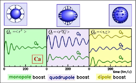
Figure 1: Evolutions of the monopole, quadrupole and dipole moments (solid lines) as a function of time for monopole (a), quadrupole (b) and dipole (c) excitations in ⁴⁰Ca.

Time dependent approaches provide an intuitive understanding of collective motions [11]. Let us for example look at the TDHF dynamics for the ⁴⁰Ca nucleus which has been initially perturbed by a collective boost. For this simulation we have used the TDHF 3D code developed by P. Bonche and coworkers [10] with the SGII Skyrme force [12].

In Fig. 1, we followed the monopole, quadrupole and dipole response for three initial conditions:

• A monopole boost using ${Q}_{0}=\frac{1}{\sqrt{4\pi}}\sum_{i}({r}_{i}^{2}-\langle{r}_{i}^{2}\rangle(t=0))$ as a boost generator. Because of the spherical symmetry, a monopole boost can only trigger monopole modes. Therefore, we only observe $\langle{Q}_{0}\rangle(t).$

• A quadrupole boost generated by ${Q}_{2}=\sum_{i}{r}_{i}^{2}Y_{0}^{2}\left({\theta}_{i},{\varphi}_{i}\right).$ The parity conservation forbids any dipole excitation when a quadrupole velocity field is applied to a spherical nucleus. Conversely, breathing modes can be triggered by the quadrupole oscillation so that we do follow both the quadrupole $\langle{Q}_{2}\rangle(t)$ and the monopole $\langle{Q}_{0}\rangle(t)$ responses.

• An isovector dipole boost induced by ${Q}_{D}=Z/A\sum_{n}z_{n}-N/A\sum_{p}z_{p}.$ This excitation can be both coupled to the quadrupole and monopole oscillations so that we monitor the three moments, $\langle{Q}_{0}\rangle(t)$, $\langle{Q}_{2}\rangle(t)$ and $\langle{Q}_{D}\rangle(t).$

3.1.1 Linear response and collective states

In Fig. 1, we observe that the collective boosts induce oscillations of the associated moments as expected from the RPA picture. They are only slightly damped in the GQR and GDR cases (fig. 1-b and 1-c respectively) while in the GMR case (fig. 1-a) beatings, characteristic of a Landau damping [11], are observed. This means that the dipole and quadrupole strengths are mostly concentrated in a single resonance while the monopole one is fragmented.

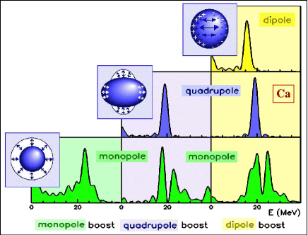
Figure 2: Monopole, quadrupole and dipole spectra obtained through the Fourier transform of the time dependent response for a monopole, quadrupole and dipole excitation in the ⁴⁰Ca.

Looking at the amplitude of the first oscillation $\langle{Q}_{\nu}\rangle_{max}$ as a function of boost strength ($k_{\nu}$) confirms the linearity of this response [13]. To get a deeper insight into the response, we study the Fourier transform $F_{\nu}(\omega)$ of $\langle{Q}_{\nu}\rangle(t)/k_{\nu}$ which is nothing but the RPA response when the velocity field $k_{\nu}$ is small enough to be in the linear regime. We see in Fig. 2 that the dipole and quadrupole modes are concentrated in a unique peak. The monopole is fragmented but the various peaks are in the same energy region so that they can be approximated by a single mode with a large Landau width.

3.1.2 Quadratic response

In Fig. 1, one can see that large amplitude dipole (fig. 1-c) and quadrupole (fig. 1-b) motion induces variations of the nucleus radius $\langle{Q}_{0}\rangle.$ Looking at the matter distribution one can see that the central density $\rho_{0}$ is affected by the dipole or quadrupole motion. Since the central density can be modified only by monopole states this imposes that the large amplitude motion gets coupled with such breathing modes. In the same way a large amplitude dipole oscillation induces a quadrupole deformation of the nuclear potential and so gets coupled with the GQR. These observations lead to the conclusion that we are in the presence of a non-linear excitation of a giant resonance (GMR or GQR, generically called $\mu$ in the following) on top of the collective motion (GQR or GDR, generically called $\nu$ in the following) initially excited through the collective boost ${Q}_{\nu}$. As expected from the quadratic response theory [13], the amplitude of the first oscillation of $\langle{Q}_{\mu}\rangle(t)$ is quadratic in the excitation velocity $k_{\nu}$ and its time dependence corresponds to $\left(\cos(\omega_{\mu}t)-1\right)$, i.e. it is initially in phase quadrature with $\langle{Q}_{\nu}\rangle(t)$ but it is oscillating with the frequency of the mode $\mu$ and not the one of the initially excited collective state $\nu$.

This interpretation is confirmed by the Fourier transform of $\langle{Q}_{\mu}\rangle(t)$ associated with the excitation of ${Q}_{\nu}$ (Fig. 2). Let us first start with the quadrupole strength non-linearly excited by a dipole boost. The observed peak is identical to the GQR-response. This is a clear indication that the observed state is indeed a GQR built on top of the GDR. It should be noticed that this frequency is different from the one of the underlying dipole motion. The monopole case is more complex because of the presence of a strong Landau spreading and it seems that the strengths of the various monopole states depend upon the considered boost. This indicates that the coupling leading to the excitation of an additional monopole state depends upon the collective mode initially excited.

3.1.3 Quadratic response and Couplings between states

$|\nu\rangle$	$\omega_{\nu}$	$q_{\nu}$	$\langle\nu|{V}|\nu 0\rangle$	$\langle\nu|{V}|\nu 2\rangle$
	(MeV)		(MeV)	(MeV)
$|0\rangle_{{}^{40}Ca}$	$22.9$	$11.6$	-	$0$
$|2\rangle_{{}^{40}Ca}$	$18.6$	$21.4$	$-4.28$	-
$|D\rangle_{{}^{40}Ca}$	$17.2$	$3.47$	$-4.58$	$-3.92$
$|0\rangle_{{}^{208}Pb}$	$15.7$	$57.1$	-	$0$
$|2\rangle_{{}^{208}Pb}$	$11.1$	$99.0$	$-2.17$	-
$|D\rangle_{{}^{208}Pb}$	$13.0$	$8.94$	$-2.40$	$-0.70$

Table 1: Energies, transition probabilities $q_{\nu}$ and coupling coefficients of the GMR, GDR and GQR in the ⁴⁰Ca and ²⁰⁸Pb. $q_{\nu}$ is expressed in fm² for the GMR and GQR and in fm for the GDR.

Assuming for each multipolarity a unique state $|\mu\rangle$ non linearly excited one can use the quadratic response theory [13] to extract the residual interaction matrix element $v_{\mu}$ between $|\nu\rangle$ and $|\nu\mu\rangle$ from the amplitudes of the induced oscillations $\langle{Q}_{\mu}\rangle_{max}$ using

$$v_{\mu}=\frac{\langle{Q}_{\mu}\rangle_{max}\omega_{\mu}}{2k_{\nu}^{2}q_{\nu}^{2}q_{\mu}}$$ (1)

where $q_{\eta}$ is the transition matrix element between the ground state $|-\rangle$ and the collective state $|\eta\rangle,$ $q_{\eta}=\langle-|Q_{\eta}|\eta\rangle,$ which can be derived from the linear response with $\eta=\nu$ since

$$q_{\nu}^{2}=\frac{\langle{Q}_{\nu}\rangle_{max}}{2k_{\nu}}.$$ (2)

The results for the ⁴⁰Ca and ²⁰⁸Pb are presented in table 1. The $\omega_{\nu}$ are computed from the time to reach the first maximum of $\langle{Q}_{\nu}\rangle(t)$. The relative sign of $v_{\mu}$ and $q_{\mu}$ is given by the early evolution of the moments ${\langle{Q}_{\mu}\rangle}$ (see Eq. 1). They appear to be all negative. The couplings $v_{\mu}$ are large of the order of few MeV. As we will see those findings are in qualitative agreement with the results of ref. [14] which is using a completely different approach.

3.2 Comparison with boson mapping calculations

$|\nu\rangle$	$J^{\pi}~{}T$	$E_{harm}$	$EWSR$	$\langle\nu|{V}|\nu 0_{1}\rangle$	$\langle\nu|{V}|\nu 0_{2}\rangle$	$\langle\nu|{V}|\nu 2\rangle$
		(MeV)	$(\%)$	(MeV)	(MeV)	(MeV)
$|0_{1}\rangle_{{}^{40}Ca}$	$0^{+}~{}0$	$18.25$	$30$	$-2.13$	$-2.36$	$-$
$|0_{2}\rangle_{{}^{40}Ca}$	$0^{+}~{}0$	$22.47$	$54$	$-2.03$	$-3.96$	$-$
$|1_{1}\rangle_{{}^{40}Ca}$	$1^{-}~{}1$	$17.78$	$56$	$-1.38$	$-2.12$	$-1.25$
$|1_{1}\rangle_{{}^{40}Ca}$	$1^{-}~{}1$	$22.03$	$10$	$-1.48$	$-2.16$	$+0.73$
$|2\rangle_{{}^{40}Ca}$	$2^{+}~{}0$	$16.91$	$85$	$-1.36$	$-2.49$	$-0.36$

Table 2: RPA one-phonon basis for the nucleus ⁴⁰Ca. For each state, spin, parity, isospin, energy and percentage of the EWSR are reported in addition to the coupling coefficients.

$|\nu\rangle$	$J^{\pi}~{}T$	$E$	$EWSR$	$\langle\nu|{V}|\nu 0_{1}\rangle$	$\langle\nu|{V}|\nu 0_{2}\rangle$	$\langle\nu|{V}|\nu 2\rangle$
		(MeV)	$(\%)$	(MeV)	(MeV)	(MeV)
$|0_{1}\rangle_{{}^{208}Pb}$	$0^{+}~{}0$	$13.61$	$61$	$-1.87$	$-0.92$	$-$
$|0_{2}\rangle_{{}^{208}Pb}$	$0^{+}~{}0$	$15.02$	$28$	$-1.32$	$-1.16$	$-$
$|1_{1}\rangle_{{}^{208}Pb}$	$1^{-}~{}1$	$12.43$	$63$	$-0.79$	$-0.59$	$-0.68$
$|1_{2}\rangle_{{}^{208}Pb}$	$1^{-}~{}1$	$16.66$	$17$	$~{}0.00$	$~{}0.00$	$-0.64$
$|2\rangle_{{}^{208}Pb}$	$2^{+}~{}0$	$11.60$	$76$	$-0.64$	$-0.48$	$-0.74$

Table 3: Same as table for the nucleus ²⁰⁸Pb.

In ref. [14] a completely different approach is used to infer the same matrix elements: the fermionic Hamiltonian is first mapped into a bosonic one making a connection between any particle-hole excitation and a boson. Because of the fermionic anticommutation relations (Pauli principle) a particle-hole excitation operator is mapped into an infinite series of boson operators. As a consequence, even if the fermionic Hamiltonian is containing only two body interaction, the boson Hamiltonian is a infinite series with many boson interactions not conserving the boson number. To be manageable this series has to be truncated and, in the application presented in [14], only the terms containing up to four boson creation or anihilation operators have been conserved. Then a RPA transformation is applied, introducing collective phonons which optimizes a harmonic picture to the system properties [15]. Using those collective degrees of freedom, the Hamiltonian then contains an harmonic part plus various interactions. An important one is the coupling between one- and two phonon states.

For practical reasons only the most collective phonons have been selected in ref. [14] some of them are presented in table 2 and 3 for ⁴⁰Ca and ²⁰⁸Pb. To illustrate their degree of collectivity the part of the energy weighted sum rule (EWSR) they are exhausting is given together with their energy. Table 2 and 3 also give the coupling matrix elements between different collective states and one of the two GMRs or the GQR built on top of them.

From the quantitative point of view, the non-linear coupling extracted from TDHF appears to be $50\%$ larger than the one reported in Table 2 and 3 [14]. This is a reasonable agreement since TDHF re-sums all the individual couplings as shown in [13]. Summing the contributions of the different collective states considered in ref. [14] reduces the difference between the reported values. However, the phonon basis studied in ref. [14] being incomplete , it is expected that the TDHF results remains higher. It should be also noticed that some differences can remain due to the approximations involved in the different approaches.

3.3 Consequences on the multiphonon spectrum

The couplings between phonon states can be used to derive the energies of the various phonon states. It appears that the very large matrix elements exciting a GMR or a GQR on top of any state are the main source of anharmonicites. As far as the two-phonon states are concerned the coupling with the three-phonon states coming from such a non-linear coupling induces an energy shift of about $2$ MeV for Ca and $1/2$ MeV for Pb. This might be the explanation of the phonon anharmonicity puzzle discussed by many authors [16, 17, 18] and summarized in [14].

4 Pre-equilibrium GDR in fusion reactions

It has been recently proposed that GR can play an essential role in fusion reactions. In particular, fusion reactions with N/Z asymmetric nuclei may lead to the excitation of a GDR because of the presence of a net dipole moment in the entrance channel [19]. Experimental indications of the possible existence of such new phenomenon have been reported in refs. [20, 21, 22] for fusion reactions and [23, 24] for deep inelastic collisions.

4.1 Collective dynamics in fusion.

As an example [25], we have computed the central collision of ${}^{20}O+^{20}Mg$ at 1 MeV per nucleon with the TDHF approach. The system rapidly fuses producing an excited ⁴⁰Ca nucleus. It presents a strong quadrupole oscillation around a slowly damped deformation. Since ²⁰O has a N over Z ratio different from this of ²⁰Mg (respectively 1.5 and 0.67), the center of mass of the protons is initially different from the neutrons one. As the time goes on this dipole moment $Q_{d}$ (i.e. the distance between the neutron and proton center of mass) oscillates (see Fig. $3$). To study the induced motion one can plot the dipole moment $Q_{{}_{d}}\$ as a function of the velocity of protons against neutrons which can be considered as its conjugated moment, $P_{{}_{d}}$. We observe a spiral in this collective phase space $(Q_{{}_{d}},P_{{}_{d}})$ , i.e. oscillations in phase quadrature of the conjugated dipole variables. This is a clear signal of the presence of a damped collective vibration.

Figure 3: Time evolution of the dipole vibration. Dipole moment $Q_{d}$ and its conjugate $P_{d}$ are plotted in the phase space (a) and $P_{d}$ is plotted in function of time (b).

The period of the observed oscillations is around $150$ fm/c while for the ⁴⁰Ca nucleus in its ground state it is almost half this value. This large difference can be explained by the deformation of the fused system. Indeed, in the TDHF simulations the compound nucleus only slowly relaxes its initial prolate elongation along the axis of the collision. The averaged value of the observed quadrupole deformation parameter is around $\varepsilon=0.23$. For symmetry reasons, the dipole oscillation occurs only along the deformation axis of the nucleus formed by fusion in head on head reactions. Therefore, a lower mean energy is expected for this longitudinal collective motion according to the following relation $E_{GDR_{Z}}=E_{GDR}\left(1-\varepsilon\right)^{2}$ The energy of the GDR along the elongation axis ${E_{GDR}}_{Z}$ fullfils this relation with $\varepsilon\approx 0.26$ in a good agreement with the previous calculation of $\varepsilon$.

4.2 Dynamical coupling of the GDR with the nucleus deformation

To get a deeper insight in the dipole oscillation observed in fusion reactions we have analyzed the time evolution of the period. From each point on the collective trajectory in the collective phase space $(Q_{{}_{d}},P_{{}_{d}})$ this quantity can be inferred from the time needed to reach the opposite side of the observed spiral (see Fig. 3). The resulting evolution is plotted in Fig. $4-a$. This period presents oscillations too. These variations of the GDR period are almost in phase with the observed oscillations of the monopole moment $Q_{0}$ and the quadrupole moment $Q_{2}$ presented in Fig. $4-b$. This points to a possible coupling between the dipole mode and another mode of vibration. The evolutions of the monopole and quadrupole moments are very similar. In particular, they present the same oscillation’s period around $166$ fm/c. Therefore, they originates from the same phenomenon, the vibration of the density around a prolate shape. This oscillation modifies the properties of the dipole mode in a time dependent way.

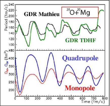
Figure 4: (a) Time behaviour of the dipole period (solid line) and its modelisation with the Mathieu’s equation (dashed line). (b) Time evolution of the monopole (dashed line) and quadrupole moments (solid line).

In order to investigate if this is the origin of the observed behavior we can model the induced mode coupling. Let us consider a harmonic oscillator of average frequency $\omega_{0}$ and let us replace the influence of the density oscillation characterized by the frequency $\omega$ by assuming that its spring constant varies in time at a frequency $\omega$. In such a model, the equation of the motion becomes the Mathieu’s equation

$$\frac{\ddot{x}}{\omega_{0}^{2}}+[1+\delta\cos(\omega t)]x=0$$ (3)

where $\omega_{0}$ is the pulsation without coupling and $\omega$ the pulsation of the density’s oscillation while $\delta$ corresponds to the magnitude of the induced frequency fluctuations. We have computed the numeric solution of Eq. 3 with the typical external frequency of the monopole and quadrupole oscillations. The bare frequency $\omega_{0}$ and the coupling strength $\delta$ have been tuned in order to get the same oscillation frequency and typical amplitude. Indeed, because the presence of the oscillating term the observed frequency is different from the bare one. The solution (see Fig. 4-a) well reproduces our observations with $\delta=-0.32$ and $\omega_{0}$ changed by a factor $1.2$ from the observed value $E_{GDR_{Z}}$. From this analysis it appears that the observed dipole motion corresponds to a giant vibration along the main axis of a fluctuating prolate shape.

4.3 Couplings between modes

It is interesting to relate $\delta$ to a coupling matrix element between collective states. Indeed, the Mathieu’s equation can be seen as the equation of motion coming from an Hamiltonian containing a coupling term between the dipole mode and the collective deformation (GMR or GQR called here after $\mu$) $V=\frac{k}{2}\delta\frac{1}{{\langle{Q}_{\mu}\rangle_{max}}}Q_{\mu}Q_{{}_{d}}^{2}.$ This leads to a coupling matrix element between the GDR and the state $\mu$ built on top of it which reads $V=\delta\frac{\omega_{0}}{2}\frac{q_{\mu}}{{\langle{Q}_{\mu}\rangle_{max}}}B_{\mu}^{\dagger}B_{d}^{\dagger}B_{{}_{d}}$. In the studied case for both the monopole and quadrupole, using the ground state matrix elements $q_{\mu},$ the amplitude of the oscillation $\frac{{\langle{Q}_{\mu}\rangle_{max}}}{q_{\mu}}$ is about $5.$ Using $\omega_{0}\simeq 13$ MeV we get a coupling between the dipole and the monopole or quadrupole $v=\delta\frac{\omega_{0}}{2}\frac{q_{\mu}}{{\langle{Q}_{\mu}\rangle_{max}}}=-0.5$ MeV. This value is qualitatively in agreement with the previous observation of a strong coupling. From a quantitative point of view, it is lower than the corresponding one (see table $1$). However, it is obtained for a hot and deformed system with a large amplitude monopole and quadrupole motion. Moreover the value derived here only correspond to the coupling with a unique mode and so should rather be compared with table 2.

5 GR in diluted nuclei

In violent heavy ion collisions, nuclear matter is excited and compressed. Then the formed nuclear system expands under the resulting thermal and mechanical pressure. Matter may also be quenched in the coexistence region of the nuclear liquid-gas phase diagram and the observed abundant fragment formation may take place through a rapid amplification of spinodal instabilities. New experimental results pleading in favor of such a spinodal decomposition have recently been reported [26, 27]. From the theoretical point of view, the spinodal instabilities in finite systems are unstable collective motions. They have been mainly studied within semi-classical or hydrodynamical framework [28, 29, 30, 31, 32]. However, since the relevant temperatures are comparable to the shell spacing and the wave numbers of the unstable modes are of the order of Fermi momentum, quantum effects are expected to be important. Quantum approaches linking the spinodal instabilities with the giant resonances can be found in [33, 34, 35].

5.1 RPA in diluted systems

To investigate instabilities encountered during the evolution of an expanding system, one should study the dynamics of the small deviations $\delta{\rho(t)}$ around the TDHF trajectory $\rho(t)$ [36]. It is more convenient to carry out such an investigation in the ”co-moving frame” and if we consider the early evolution of instabilities in the vicinity of an initial state the problem reduces to an RPA like equation [35]. Then, small density fluctuations are characterized by the RPA modes $\rho_{\nu}$ and the associated frequencies $\omega_{\nu}$. When the frequency of a mode drops to zero and then becomes imaginary, the system enters an instability region.

In order to perform an extensive study of instabilities we may parametrize the possible densities $\rho_{0}$ either by a static Hartree-Fock (HF) calculations constrained by a set of collective operators [37], or using a direct parameterization of the density matrix. In the following, we follow the second approach by introducing a self-similar scaling of the HF density as suggested by dynamical simulations.

First, we solve the HF equation for the ground state $\left[h_{HF},\rho_{HF}\right]=0$, leading to the single-particle wave functions $|\varphi_{i}\rangle$ and the associated energies $\varepsilon_{i}$. Then we introduce the density matrix at a finite temperature $T$ as $\rho_{HF}\left[T\right]=1/\left(1+\exp\left(\left(h_{HF}\frac{\;}{\;}\varepsilon_{F}\left[T\right]\right)/T\right)\right)$, where $\varepsilon_{F}\left[T\right]$ is the corresponding Fermi level that is tuned in order to get the correct particle number. Then, we perform a scaling transformation, $R\left[\alpha\right],$ which inflates the wave functions in radial direction by a factor $\alpha$ according to $\langle r|R\left[\alpha\right]|\varphi\rangle=\alpha^{-1/3}\langle r/\alpha|\varphi\rangle.$ We then define the density matrix for a hot and diluted system by $\rho_{0}\left[\alpha,T\right]=R\left[\alpha\right]\;\rho_{HF}\left[\alpha^{2}T\right]\;R^{\dagger}\left[\alpha\right]$. The eigenstates of the constrained Hamiltonian are given by $|i\rangle=R\left[\alpha\right]|\varphi_{i}\rangle$, and the corresponding energies and occupation numbers are $\epsilon_{i}=\varepsilon_{i}/\alpha^{2}$ and $n_{i}=1/\left(1+\exp\left(\left(\varepsilon_{i}\frac{\;}{\;}\varepsilon_{F}\left[\alpha^{2}T\right]\right)/\alpha^{2}T\right)\right)$, respectively (see Ref. [35] for more details).

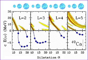
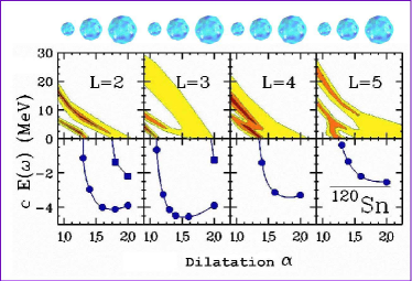
Figure 5: Contour plots of the isoscalar strength functions associated with the multipolarity $L=2-5$ as a function of the dilution parameter $\alpha$ and the collective energy of the mode $E_{\nu}=c\hbar\omega_{\nu}$ ($c=1$ for stable modes, $-i$ for unstable modes) for ⁴⁰Ca (left) and ¹²⁰Sn (right).

We performed the HF calculations in the coordinate representation using the Skyrme force SLy4 [38]. The particle and hole states are obtained by diagonalizing the HF Hamiltonian in a large harmonic oscillator representation [39], which includes 12 major shells for Ca isotopes and 15 for Sn. We apply the scaling and heating procedures described above to the density matrix, and calculate the residual interaction in a self consistent manner. We solve the RPA by a direct diagonalization using a discrete two quasi-particle excitation representation [40].

5.2 Dilution-dependent GR frequencies

The top part of Fig. 5 shows calculations performed for ⁴⁰Ca. Top panels shows contour plots of the isoscalar strength function associated with the isoscalar operator $A_{LM}^{s}=\sum_{i=1}^{A}r_{i}^{L}Y_{LM}$, with multipolarity $L=2-5$, as a function of the dilution parameter $\alpha$. We observe that, in the stable domain, the energy associated with the dominant isoscalar strength decreases as dilution becomes larger, and at a critical dilution it drops to zero. At larger dilution, the system becomes unstable, and for each multipolarity, one or two unstable modes appear. This is illustrated in the bottom panel, where the ”imaginary energy” of the mode $E_{\nu}=-i\hbar\omega_{\nu}$ is plotted as a function of the dilution. Looking at the RPA solution in the coordinate space, it appears that the collective motions transform into volume modes when they become unstable. We observe in fact a quite complex structure of the unstable modes: Volume and surface instabilities are generally coupled, as well as isoscalar and isovector excitations, since protons and neutrons move in oposite way [35].

5.3 RPA-instabilities ”phase diagram”

We, also, carry out calculations at finite temperature and determine the dilutions at which different unstable modes begin to appear. This allows us to specify the border of the instability region in the density-temperature plane for different unstable modes. Fig. 4 shows phase diagrams for octupole instabilities in ¹²⁰Sn.

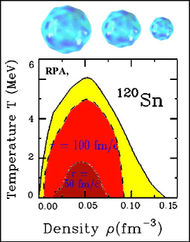
Figure 6: Border of the instability region (full fine) associated with $L=3$, for ¹²⁰Sn. The dashed line connects the points having the instability growth time $\tau$ = 100 fm/c. The dots are associated with $\tau$ = 50 fm/c.

Here, for simplicity, we define the density as $\rho=\rho_{0}/{\alpha}^{3}$. The full line indicates the border of the instability region. The dashed line connects points that are associated with the instability growth time $\tau$ = 100 fm/c, and the dots correspond to situations with a shorter growth time $\tau$ = 50 fm/c. We observe that in finite nuclei the instability region is quite reduced as compared to that of nuclear matter. The limiting temperature for instability to occur is around 6 MeV for Sn and 4.5 MeV for Ca (see [35]) while it is about $16$ MeV in symmetric nuclear matter. As a result, heavier systems have larger instability region than the lighter ones.

5.4 Link with the coupling between modes

The observed dilution dependence of the GR’s energies can be interpreted in terms of a coupling between the studied GR and the GMR. Indeed, it corresponds to the Hamiltonian $H=\omega\left(\alpha\right)B_{d}^{\dagger}B_{{}_{d}}$ where $\omega\left(\alpha\right)$ is the GR frequency for a dilution $\alpha$. Using a Taylor expansion of $\omega\left(\alpha\right)$ around $\alpha=1$ and introducing $\varepsilon=\alpha-1,$ $\omega\left(\alpha\right)=\omega_{0}+\varepsilon\left.\partial_{\alpha}\omega\right|_{0},$ and the Hamiltonian becomes $H=\omega_{0}B_{d}^{\dagger}B_{{}_{d}}+\varepsilon\left.\partial_{\alpha}\omega\right|_{0}B_{d}^{\dagger}B_{{}_{d}}.$ The dilution factor $\alpha$ can be related to the collective observables using $\langle r^{2}\rangle=\alpha^{2}\langle r^{2}\rangle_{0}\simeq\langle r^{2}\rangle_{0}+2\varepsilon\langle r^{2}\rangle_{0}$ and $Q_{\mu}=\frac{1}{\sqrt{4\pi}}\left(r^{2}-\langle r^{2}\rangle_{0}\right)=q_{\mu}\left(B_{\mu}^{\dagger}+B_{\mu}\right)$ so that the Hamiltonian reads $H=\omega_{0}B_{d}^{\dagger}B_{{}_{d}}+\left[\frac{\sqrt{4\pi}q_{\mu}}{2\langle r^{2}\rangle_{0}}\left.\partial_{\alpha}\omega\right|_{0}B_{\mu}^{\dagger}B_{d}^{\dagger}B_{{}_{d}}+h.c.\right]$. This leads to a coupling matrix element between the GR and a GMR ($\mu$) built on top of it which reads $V=\frac{\sqrt{4\pi}q_{\mu}}{2\langle r^{2}\rangle_{0}}\left.\partial_{\alpha}\omega\right|_{0}B_{\mu}^{\dagger}B_{d}^{\dagger}B_{{}_{d}}$. Looking at the GQR decrease with the dilution, we get $\partial_{\alpha}\omega\simeq-40$ MeV for ⁴⁰Ca. Using the transition matrix element for the GMR extracted in table 1, $q_{\mu}\simeq 12$ fm², and $\langle r^{2}\rangle_{0}/\sqrt{4\pi}\simeq 125$ fm² we get $v_{\mu}=\frac{q_{\mu}}{2\langle r^{2}\rangle_{0}/\sqrt{4\pi}}\left.\partial_{\alpha}\omega\right|_{0}$ $\simeq-2$ MeV. This value is qualitatively in agreement with the previous observation of a strong coupling. In particular we understand the sign of the interaction since the energy of the modes is reduced in a diluted system ($v_{\mu}<0$). From a quantitative point of view, it is a factor 2 lower than the one reproduced in table $1$. However one should remember that we compute here an average matrix element while in table 1 it is more an integrated one. In fact this result should be compared to the one in table 2 and indeed they are in excellent agreement.

6 Conclusion

In conclusion, we have presented a study of 3 different situations: the excitation of small amplitude motions and the coupling between phonon states, the excitation of pre-equilibrium GDR in fusion reaction and the modification of the GDR properties due to the dynamics of the monopole and quadrupole deformation and finally the early development of spinodal instabilities. The 3 phenomena show that collective modes are strongly coupled to the monopole (and quadrupole) degrees of freedom. We have presented original methods to extract the coupling matrix element between a collective mode and a GMR (or GQR) built on top of it. The 3 studied phenomena are in qualitative agreement pointing to a negative coupling of the order of the MeV. The quantitative difference we observe which might come the differences between the 3 studied cases is now under study.

References

- [1] A. Bohr and B. Mottelson, Nuclear Structure Vol II, Benjamin (N.Y.), (1975).
- [2] M. N. Harakeh and A. van der Woude, Giant Resonances: Fundamental High-Frequency Modes of Nuclear Excitation, Oxford Science publications (2001).
- [3] G. C. Baldwin and G. Klaiber, Phys. Rev. 71, 3 (1947).
- [4] M. Goldhaber and E. Teller, Phys. Rev. 74, 1046 (1948).
- [5] S. Fukuda and Y. Torizuka, Phys. Rev. Lett. 29, 1109 (1972).
- [6] N. Marty et al, Orsay report IPNO76-03; M. N. Harakeh, K. van der Borg et al, Phys. Rev. Lett. 38, 676 (1977); D. H. Youngblood et al, Phys. Rev. Lett. 39, 1188 (1977).
- [7] A. Van der Woude, Prog. in Part. and Nucl. Phys. 18, 217 (1987).
- [8] J. O. Newton, B. Herskind, R. M. Diamond, E. L. Dines, J. E. Draper, K. L. Lindenberger, C. Schuck, S. Shih and F. S. Stephens, Phys. Rev. Lett. 46, 138 (1981).
- [9] P. Ring and P. Schuck, The Nuclear many body problem, Springer-Verlag N. Y. (1981).
- [10] K.-H. Kim, T. Otsuka and P. Bonche, J. Phys. G23, 1267 (1997).
- [11] Ph. Chomaz, N. V. Giai and S. Stringari, Phys. Lett. B189, 375 (1987).
- [12] N. V. Giai and H. Sagawa, Nucl. Phys. A371, 1 (1981).
- [13] C. Simenel and Ph. Chomaz, Phys. Rev. C68, 024302 (2003).
- [14] M. Fallot et al., nucl-th/0111013, submitted.
- [15] D. Beaumel and Ph. Chomaz, Phys. Lett. B277, 1 (1992).
- [16] Ph. Chomaz and N. Frascaria, Phys. Rep. 252, 275 (1995).
- [17] H. Emling, Prog. Part. Nucl. Phys. 33, 729 (1994).
- [18] T. Aumann et al., Annu. Rev. Nucl. Sci. 48, 351 (1998).
- [19] Ph. Chomaz et al., Nucl. Phys. A563, 509 (1993).
- [20] S. Flibote et al., Phys. Rev. Lett. 77, 1448 (1996).
- [21] F. Amorini et al., Phys. Rev. C58, 987 (1998).
- [22] D. Pierroutsakou et al., Nucl. Phys. A687, 245c (2001).
- [23] M. Sandoli et al., Eur. Phys. J. A6, 275 (1999)
- [24] M. Papa et al., Eur. Phys. J. A4, 69 (1999).
- [25] C. Simenel, Ph. Chomaz and G. De France, Phys. Rev. Lett. 86, 2971 (2001).
- [26] L. Beaulieau et al., Phys. Rev. Lett. 84, 5971 (2000).
- [27] B. Borderie et al., Phys. Rev. Lett. 86, 3252 (2001).
- [28] G. F. Bertsch and P. J. Siemens, Phys. Lett. B126 , 9 (1983).
- [29] H. Heiselberg, C. J. Pethick and D. G. Ravenhall, Phys. Rev. Lett. 61, 818 (1988).
- [30] W. Nörenberg, G. Papp and P. Rozmej, Eur. Phys. J. A9, 327 (2000).
- [31] M. Colonna, Ph. Chomaz, and J. Randrup, Nucl. Phys. A567, 637 (1994); A. Guarnera, M. Colonna and Ph. Chomaz, Phys. Lett. B373, 267 (1996).
- [32] B. Jacquot, S. Ayik, Ph. Chomaz and M. Colonna, Phys. Lett. B383, 247 (1996).
- [33] S. Ayik, M. Colonna and Ph. Chomaz, Phys. Lett. B353 , 417 (1995).
- [34] B. Jacquot, M. Colonna, S. Ayik and Ph. Chomaz, Nucl. Phys. A617, 356 (1997).
- [35] M. Colonna, Ph. Chomaz and S. Ayik, Phys. Rev. Lett. 88, 122701 (2002).
- [36] D. Vautherin and M. Veneroni, First Int. Spring Seminar on Nuclear Physics, Sorrento, Italy (1986).
- [37] H. Sagawa and G. F. Bertsch, Phys. Lett. B146, 138 (1984); B155, 11 (1985).
- [38] E. Chabanat et al., Nucl. Phys. A627, 710 (1997); Nucl. Phys. A635, 231 (1997); Erratum: Nucl. Phys. A643, 441 (1998).
- [39] N. Van Giai and H. Sagawa, Nucl. Phys. A371,1 (1981).
- [40] D. Vautherin and N. Vinh Mau, Nucl. Phys. A422 , 140 (1984).
- [41] Bao-An Li, C. M. Ko, Nucl. Phys. A 618 498 (1997); V. Baran, M. Colonna, M. Di Toro and V. Greco, Phys. Rev. Lett. 86, 4492 (2001).