Abstract

The effect of deformation on the two-neutrino double decay ($2\nu\beta\beta$-decay) for ground state transition ${}^{76}Ge\rightarrow{{}^{76}Se}$ is studied in the framework of the deformed QRPA with separable Gamow-Teller residual interaction. A new suppression mechanism of the $2\nu\beta\beta$-decay matrix element based on the difference in deformations of the initial and final nuclei is included. An advantage of this suppression mechanism in comparison with that associated with ground state correlations is that it allows a simultaneous description of the single $\beta$ and the $2\nu\beta\beta$-decay. By performing a detail calculation of the $2\nu\beta\beta$-decay of ${}^{76}Ge$, it is found that the states of intermediate nucleus lying in the region of the Gamow-Teller resonance contribute significantly to the matrix element of this process.

PACS numbers:23.40.BW,23.40.HC

1 Introduction

There is a continuous attempt to improve the accuracy and reliability of the calculated single beta ($\beta$) and double beta ($\beta\beta$) decay nuclear matrix elements . Their values affect our understanding of astrophysical processes and the fundamental properties of neutrino, in particular neutrino mixing and masses.

The complexity of the calculation of the double beta decay matrix elements consists in the fact that it is a second order process, i.e., in addition to the initial and final nuclear states the knowledge of the complete set of the states of the intermediate nucleus is required. In solving of this problem different models as well as different nuclear structure scenarios were applied [1, 2, 3].

Double beta decay can occur in different modes: The neutrinoless mode ($0\nu\beta\beta$-decay) requires violation of the lepton number and probes new physics scenarios beyond the Standard Model (SM) of particle physics [1, 2, 4, 5, 6, 7] . The two-neutrino decay ($2\nu\beta\beta$-decay) mode is process allowed in the SM, i.e., the half-life of this process is free of unknown parameters of the particle physics side [1, 2, 3, 4].

As the half-lifes of the $2\nu\beta\beta$-decay have been already measured for about ten nuclei, the values of the associated nuclear matrix element can be extracted directly. It provides a cross-check on the reliability of the matrix element calculations.

Since the nuclei undergoing double beta decay are open shell nuclei the proton-neutron Quasiparticle Random Phase Approximation (pn-QRPA) method has been the most employed in the evaluation of the double beta decay matrix elements [1, 2]. In addition, this approach has succeeded in reproducing the experimentally observed suppression of the $2\nu\beta\beta$-decay transitions [10, 11, 12]. However, a strong sensitivity of the computed matrix elements on an increase of the strength of the particle-particle residual interaction in the $1^{+}$ channel leads to a problem of fixing this parameter [1]. Thus various refinements of the original pn-QRPA have been advanced.

In the last decade the extensions of the pn-QRPA, which include proton-neutron pairing (full-QRPA) [13], a partial restoration of the Pauli exclusion principle discarded in the pn-QRPA (renormalized QRPA) [14, 15] and higher order RPA corrections [16, 17], have received much attention in the context of the nuclear structure calculations for the double beta decay. In spite of the fact that these alterations of the pn-QRPA improved reliability of the evaluated matrix elements, further progress of the nuclear approaches dealing with double beta decay is needed.

The deformation degrees of freedom of nuclei undergoing the $2\nu\beta\beta$-decay were first considered within Nilsson model with pairing [18]. Bogdan, Faessler, Petrovici and Holan calculated the $0\nu\beta\beta$-decay in the pairing model including deformation and rotation [19]. The first QRPA calculation of the $2\nu\beta\beta$-decay matrix elements in a deformed Nilsson-BCS basis were presented in Ref. [20]. The authors did not take into account particle-particle interaction of the nuclear Hamiltonian and assumed initial and final nuclei to be equally deformed. The effects of nuclear deformation were considered also within the $SU(3)$ scheme [21], which has been found successfull in describing the heavy rotational nuclei. The $SU(3)$ scheme is a tractable shell model theory for deformed nuclei, which requires a severe truncation of the single particle basis. This approach was used for calculation of the double beta decay half-lifes of different heavy nuclear systems [22] and the predictions were found to be in good agreement with available experimental data for ${}^{150}Nd$ and ${}^{238}U$ [8]. The effect of the deformation of the nuclear shape on the two-neutrino double beta decay matrix element has been discussed in details within a method developed by Raduta, Faessler and Delion [23]. The authors used angular momentum projected single particle basis having the energies close to those of Nilsson levels. The Gamow-Teller states were generated with help of the spherical proton-neutron QRPA with a good angular momentum quantum number within the considered basis. The results were presented for the $2\nu\beta\beta$-decay of ${}^{82}Se$. It was shown that the deformation affects significantly the $2\nu\beta\beta$-decay matrix element. The deformation effect on the double Gamow-Teller matrix element of ${}^{100}Mo$ were investigated in the Hartree–Fock–Bogoliubov (HFB) framework in Ref. [24]. It was noticed that there is a necessity of an appropriate amount of deformation in the HFB intrinsic state to reproduce the experimental $2\nu\beta\beta$-decay half-life.

There is an interest to study the effect of deformation on the double beta decay matrix elements within the deformed QRPA [25, 26], which allows unified description of the $2\nu\beta\beta$-decay in spherical and deformed nuclei. This nuclear structure aproach has been found succeessful in description of the single $\beta$-decay transitions of medium and heavy nuclei a long time ago. In the first applications only the particle-hole terms of the Gamow-Teller force were taken into account [25, 26]. It was supposed that the particle-particle terms have minor effect on the Gamow-Teller strength function. However, from the spherical QRPA calculations we know that the particle-particle force plays an important role for describing the $\beta^{+}$- and $\beta\beta$-processes [10, 11, 12]. Recently, the importance of the particle-particle interaction has been confirmed also in the deformed QRPA treatment of the Gamow-Teller strength distributions [27]. A strong sensitivity of the single $\beta$-decay characteristics to the nuclear shape, RPA ground state correlations and pairing correlations were manifested.

The aim of the present paper is to investigate the effect of nuclear deformation on the double Gamow-Teller matrix element of the $2\nu\beta\beta$-decay within the deformed QRPA. We present here as an example numerical results for the $2\nu\beta\beta$-decay of ${}^{76}Ge$, which is a prominent transition due to ongoing and planned $\beta\beta$ experiments for this isotope [28, 29]. A subject of our interest is also the $\beta^{-}$ and $\beta^{+}$ distributions in ${}^{76}Ge$ and ${}^{76}Se$, respectively. The problem of fixing of the nuclear structure parameters will be addressed.

The paper is organized as follows. The basic elements of the deformed QRPA formalism are reviewed in Section 2. In Section 3 we establish our choice for deformation, pairing and force parameters. Then the results for the $2\nu\beta\beta$-decay ground state transition ${}^{76}Ge\rightarrow^{76}Se$ are analyzed in context of the Gamow-Teller strength distributions of ${}^{76}Ge$ and ${}^{76}Se$. The final conclusions and remarks are pointed out in Section IV.

2 Formalism of the deformed QRPA

The theoretical approach is based on the deformed proton-neutron Quasiparticle Random Phase Approximation with separable proton-neutron residual interaction, which is relevant for the allowed Gamow-Teller transitions [25, 26, 27]. This approach allows for an unified description of the $2\nu\beta\beta$-decay process in deformed and spherical nuclei.

The total nuclear Hamiltonian takes the form

$$H=H_{0}+H_{int}.$$ (1)

$H_{0}$ denotes the Hamiltonian for the quasiparticle mean field described by a deformed axially-symmetric Woods-Saxon potential [36]

$$H_{0}=\sum_{\tau\rho}E_{\tau}a^{\dagger}_{\tau\rho_{\tau}}a_{\tau\rho_{\tau}}(\tau=p,n),$$ (2)

where $E_{\tau}$ are the quasiparticle energies. $a^{+}_{\tau\rho_{\tau}}$ ($a^{+}_{\tau\rho_{\tau}}$) is the quasiparticle creation (annihilation) operator. The p (n) index denotes proton (neutron) quasiparticle states with projection $\Omega_{p}$ ($\Omega_{n}$) of the full angular momentum on the nuclear symmetry axis and parity $\pi_{p}$ ($\pi_{n}$). The index $\rho$ ($\rho=\pm 1$) represents the sign of the angular momentum projection $\Omega$. We note that intrinsic states are twofold degenerate. The states with $\Omega_{\tau}$ and $-\Omega_{\tau}$ have the same energy as consequence of the time reversal invariance. We shall use notation such that $\Omega_{\tau}$ is taken to be positive for states and negative for time reversed states.

The method includes pairing between like nucleons in the BCS approximation with fixed gap parameters for protons, $\Delta_{p}$, and neutrons, $\Delta_{n}$.

$$~{}~{}~{}E_{\tau}=\sqrt{(\varepsilon_{\tau}-\lambda_{\tau})^{2}+\Delta^{2}_{\tau}},$$ (3)

where $\varepsilon_{\tau}$ are single–particle energies, $\Delta_{\tau}$ is the gap, $\lambda_{\tau}$ is the Fermi energy. The Bogolyubov transformation, which defines the quasiparticle representation, is given by

$$\left(\matrix{c^{\dagger}_{\tau\rho_{\tau}}\cr\tilde{c}_{\tau\rho_{\tau}}}\right)=\left(\matrix{u_{\tau}&v_{\tau}\cr-v_{\tau}&u_{\tau}}\right)\left(\matrix{a^{\dagger}_{\tau\rho_{\tau}}\cr\tilde{a}_{\tau\rho_{\tau}}}\right).$$ (4)

Here, $c^{\dagger}_{\tau\rho_{\tau}}$ and $c_{\tau\rho_{\tau}}$ are creation and annihilation operators for particles, respectively. $\sim$ indicates the single nucleon state obtained by the time reversal operator $T=Ke^{-i\sigma_{y}\pi/2}=\left(\matrix{0&-1\cr 1&0}\right)K$. This state is given in the Appendix A [37]. The occupation probabilities $v^{2}_{\tau}$ are written as

$$v^{2}_{\tau}=\frac{1}{2}\left(1-\frac{\varepsilon_{\tau}-\lambda_{\tau}}{E_{\tau}}\right),~{}~{}~{}u^{2}_{\tau}=1-v^{2}_{\tau}$$ (5)

and the proton and neutron number equations are

$$Z=2\sum_{p}v^{2}_{p},~{}~{}~{}~{}~{}~{}N=2\sum_{n}v^{2}_{n},$$ (6)

where Z and N are the numbers of protons and neutrons, respectively.

The residual interaction part $H_{int}$ of nuclear Hamiltonian in Eq. (1) contains two terms associated with particle–hole (ph) and particle–particle (pp) interaction:

$$H_{int}=~{}~{}\chi\sum_{K=0,\pm 1}(-1)^{K}(\beta^{-}_{1K}\beta^{+}_{1-K}+\beta^{+}_{1-K}\beta^{-}_{1K})~{}-\kappa\sum_{K=0,\pm 1}(-1)^{K}(P^{-}_{1K}P^{+}_{1-K}+P^{+}_{1-K}P^{-}_{1K}).$$ (7)

The operators $\beta^{-}$ and $P^{-}$ are ph and pp components of the spin-isospin $\tau^{+}\sigma$, namely,

$$\beta^{-}_{K} = \sum_{p\rho_{p}n\rho_{n}}<p\rho_{p}|\tau^{+}\sigma_{K}|n\rho_{n}>c^{\dagger}_{p\rho_{p}}c_{n\rho_{n}},~{}~{}~{}\beta^{+}_{K}=(\beta^{-}_{K})^{\dagger},$$

$$P^{-}_{K} = \sum_{p\rho_{p}n\rho_{n}}<p\rho_{p}|\tau^{+}\sigma_{K}|n\rho_{n}>c^{\dagger}_{p\rho_{p}}{\tilde{c}}^{\dagger}_{n\rho_{n}},~{}~{}~{}P^{+}_{K}=(P^{-}_{K})^{\dagger}.$$ (8)

The ph and pp forces in Eq. (6) are defined to be repulsive and attractive ($\chi,\kappa\geq 0$), respectively, reflecting the general feature of the nucleon-nucleon interaction in the $J^{\pi}=1^{+}$ channel. The explicit form of the matrix element $<p\rho_{p}|\tau^{+}\sigma_{K}|n\rho_{n}>$ is presented in the Appendix A.

After neglecting the scattering terms $a^{\dagger}_{p\rho_{p}}a_{n\rho_{n}}$ and $a^{\dagger}_{n\rho_{n}}a_{p\rho_{p}}$ the quasiparticle representation of $H_{int}$ takes the form

$$H_{int} = ~{}~{}~{}\chi\sum_{K=0,\pm 1}\sum_{ij}[(\sigma_{K}(i){\overline{\sigma}}_{K}(j)+{\overline{\sigma}}_{K}(i)\sigma_{K}(j))(A^{\dagger}(i,K)A^{\dagger}({\bar{j}},K)+A({\bar{j}},K)A(i,K))$$ (9)

$$~{}~{}~{}~{}~{}~{}~{}~{}~{}~{}+~{}(\sigma_{K}(i){{\sigma}}_{K}(j)+{\overline{\sigma}}_{K}(i){\overline{\sigma}}_{K}(j))(A^{\dagger}(i,K)A(j,K)+A(j,K)A^{\dagger}(i,K))]$$

$$~{}-\kappa\sum_{K=0,\pm 1}\sum_{ij}[-(\pi_{K}(i){\overline{\pi}}_{K}(j)+{\overline{\pi}}_{K}(i)\pi_{K}(j))(A^{\dagger}(i,K)A^{\dagger}({\bar{j}},K)+A({\bar{j}},K)A(i,K))$$

$$~{}~{}~{}~{}~{}~{}~{}~{}~{}~{}+~{}(\pi_{K}(i){{\pi}}_{K}(j)+{\overline{\pi}}_{K}(i){\overline{\pi}}_{K}(j))(A^{\dagger}(i,K)A(j,K)+A(j,K)A^{\dagger}(i,K))],$$

with

$$\sigma_{K}(i) = <p\rho_{p}|\tau^{+}\sigma_{K}|n\rho_{n}>u_{p}v_{n},~{}~{}{\overline{\sigma}}_{K}(i)=<p\rho_{p}|\tau^{+}\sigma_{K}|n\rho_{n}>v_{p}u_{n},$$

$$\pi_{K}(i) = <p\rho_{p}|\tau^{+}\sigma_{K}|n\rho_{n}>u_{p}u_{n},~{}~{}{\overline{\pi}}_{K}(i)=<p\rho_{p}|\tau^{+}\sigma_{K}|n\rho_{n}>v_{p}v_{n}.$$ (10)

$A^{\dagger}_{i}$ and $A_{i}$ are the two-quasiparticle creation and annihilation operators

$$A^{\dagger}(i,K)=a^{\dagger}_{p\rho_{p}}a^{\dagger}_{n\rho_{n}},~{}~{}A^{\dagger}({\bar{i}},K)={\tilde{a}}^{\dagger}_{p\rho_{p}}{\tilde{a}}^{\dagger}_{n\rho_{n}},~{}~{}A(i,K)=(A^{\dagger}(i,K))^{\dagger}.$$ (11)

The quasiparticle pairs $i$ and ${\bar{i}}$ are defined by the selection rules $\Omega_{p}-\Omega_{n}=K$ and $\Omega_{n}-\Omega_{p}=K$, respectively, and $\pi_{p}\pi_{n}=1.$

The above considered model Hamiltonian includes terms with $K=0,\pm 1$ and describes $J^{\pi}K=1^{+}1,1^{+}0$ excitations. In the laboratory frame the proton-neutron QRPA phonon wave functions for Gamow-Teller excitations in even-even nuclei have the form

$$|1M(K),m> = \sqrt{\frac{3}{16\pi^{2}}}[{\cal D}^{1}_{MK}(\phi,\theta,\psi){Q^{m}_{K}}^{\dagger}+(-1)^{1+K}{\cal D}^{1}_{M-K}(\phi,\theta,\psi){Q^{m}_{-K}}^{\dagger}]|rpa>~{}~{}~{}(K=\pm 1),$$

$$|1M(K),m> = \sqrt{\frac{3}{8\pi^{2}}}{\cal D}^{1}_{MK}(\phi,\theta,\psi){Q^{m}_{K}}^{\dagger}|rpa>~{}~{}~{}(K=0),$$ (12)

where $|rpa>$ denotes the QRPA ground state. The intrinsic states are generated by the phonon creation operator

$${Q^{m}_{K}}^{\dagger}=\sum_{i}[X^{m}_{i,K}A^{\dagger}(i,K)-Y^{m}_{i,K}A({\bar{i}},K)].$$ (13)

In the case $K=\pm 1$ ($K=0$) the sum in Eq. (13) includes all bound and quasibound two-quasiparticle spin–projection–flip (non–spin–projection–flip) configurations. We note that the $K=-1$ and $K=1$ modes are related to each other through time reversal and are degenerate.

The excitation energy $\omega_{k}$ and the amplitudes $X^{m}_{i,K}$ and $Y^{m}_{i,K}$ of the phonon ${Q^{m}_{K}}^{\dagger}$ are obtained by solving the RPA matrix equation

$$\left(\matrix{{\cal A}(K)&{\cal B}(K)\cr{\cal B}(K)&{\cal A}(K)}\right)~{}\left(\matrix{X^{m}_{K}\cr Y^{m}_{K}}\right)~{}=~{}\omega^{m}_{K}~{}\left(\matrix{1&0\cr 0&-1}\right)~{}\left(\matrix{X^{m}_{K}\cr Y^{m}_{K}}\right),$$ (14)

where

$${\cal A}_{ij}(K) = {\cal E}_{i}\delta_{ij}+2\chi[\sigma_{K}(i)\sigma_{K}(j)+{\overline{\sigma}}_{K}(i){\overline{\sigma}}_{K}(j)]-2\kappa[\pi_{K}(i)\pi_{K}(j)+{\overline{\pi}}_{K}(i){\overline{\pi}}_{K}(j)],$$

$${\cal B}_{ij}(K) = ~{}~{}~{}~{}~{}~{}~{}~{}~{}~{}~{}2\chi[\sigma_{K}(i){\overline{\sigma}}_{K}(j)+{\overline{\sigma}}_{K}(i)\sigma_{K}(j)]+2\kappa[\pi_{K}(i){\overline{\pi}}_{K}(j)+{\overline{\pi}}_{K}(i)\pi_{K}(j)]$$ (15)

with ${\cal E}_{i}=E_{p}+E_{n}$ the two-quasiparticle excitation energy.

An advantage of using the separable forces is that the RPA matrix equation reduces to a homogeneous system of only four equations for the four unknown norms $N_{\sigma}$, $N_{\bar{\sigma}}$, $N_{\pi}$ and $N_{\bar{\pi}}$, which is much easier to solve in comparison with the full diagonalization of RPA matrix of large dimension. The corresponding secular equation is given by

$$\left|\matrix{1+\chi(-P^{K}_{\sigma\sigma}+R^{K}_{\bar{\sigma}\bar{\sigma}})~{}&~{}\chi(-P^{K}_{\sigma\bar{\sigma}}+R^{K}_{\bar{\sigma}\sigma})~{}&~{}\kappa(P^{K}_{\sigma\pi}+R^{K}_{\bar{\sigma}\bar{\pi}})~{}&~{}\kappa(P^{K}_{\sigma\bar{\pi}}+R^{K}_{\bar{\sigma}\pi})\cr\chi(-P^{K}_{\bar{\sigma}\sigma}+R^{K}_{\sigma\bar{\sigma}})~{}&~{}1+\chi(-P^{K}_{\bar{\sigma}\bar{\sigma}}+R^{K}_{\sigma\sigma})~{}&~{}\kappa(P^{K}_{\bar{\sigma}\pi}+R^{K}_{\sigma\bar{\pi}})~{}&~{}\kappa(P^{K}_{\bar{\sigma}\bar{\pi}}+R^{K}_{\sigma\pi})\cr\chi(-P^{K}_{\pi\sigma}-R^{K}_{\bar{\pi}\bar{\sigma}})~{}&~{}\chi(-P^{K}_{\pi\bar{\sigma}}-R^{K}_{\bar{\pi}\sigma})~{}&~{}1+\kappa(P^{K}_{\pi\pi}-R^{K}_{\bar{\pi}\bar{\pi}})~{}&~{}\kappa(P^{K}_{\pi\bar{\pi}}-R^{K}_{\bar{\pi}\pi})\cr\chi(-P^{K}_{\bar{\pi}\sigma}-R^{K}_{\pi\bar{\sigma}})~{}&~{}\chi(-P^{K}_{\bar{\pi}\bar{\sigma}}-R^{K}_{\pi\sigma})~{}&~{}\kappa(P^{K}_{\bar{\pi}\pi}-R^{K}_{\pi\bar{\pi}})~{}&~{}1+\kappa(P^{K}_{\bar{\pi}\bar{\pi}}-R^{K}_{\pi\pi})}\right|=0,$$ (16)

with

$$P^{K}_{\alpha\acute{\alpha}}=2\sum_{i}\frac{\alpha(i)\acute{\alpha}(i)}{\omega^{m}_{K}-{\cal E}_{i}},~{}~{}~{}~{}~{}R^{K}_{\alpha\acute{\alpha}}=2\sum_{i}\frac{\alpha(i)\acute{\alpha}(i)}{\omega^{m}_{K}+{\cal E}_{i}},~{}~{}~{}~{}(\alpha,\acute{\alpha}=\sigma,\bar{\sigma},\pi,\bar{\pi}).$$ (17)

The forward and backward amplitudes are written as

$$X^{m}_{iK} = \frac{2N_{\sigma}}{\omega^{m}_{K}-{\cal E}_{i}}[~{}\chi({\sigma_{K}(i)}+{{\bar{\sigma}}_{K}(i)}\frac{N_{\bar{\sigma}}}{N_{\sigma}})-\kappa({\pi_{K}(i)}\frac{N_{\pi}}{N_{\sigma}}+{{\bar{\pi}}_{K}(i)}\frac{N_{\bar{\sigma}}}{N_{\sigma}})~{}],$$

$$Y^{m}_{iK} = \frac{-2N_{\sigma}}{\omega^{m}_{K}+{\cal E}_{i}}[~{}\chi({{\bar{\sigma}}_{K}(i)}+{{{\sigma}}_{K}(i)}\frac{N_{\bar{\sigma}}}{N_{\sigma}})+\kappa({{\bar{\pi}}_{K}(i)}\frac{N_{\pi}}{N_{\sigma}}+{{{\pi}}_{K}(i)}\frac{N_{\bar{\sigma}}}{N_{\sigma}})~{}],$$ (18)

where for the norms $N_{\sigma}$, $N_{\bar{\sigma}}$, $N_{\pi}$ and $N_{\bar{\pi}}$ we have

$$N_{\sigma} = \sum_{j}[\sigma_{K}(i)X^{m}_{jK}+{\bar{\sigma}}_{K}(i)Y^{m}_{jK}],~{}~{}~{}N_{\bar{\sigma}}=\sum_{j}[{\bar{\sigma}}_{K}(i)X^{m}_{jK}+\sigma_{K}(i)Y^{m}_{jK}],$$

$$N_{\pi} = \sum_{j}[\pi_{K}(i)X^{m}_{jK}-{\bar{\pi}}_{K}(i)Y^{m}_{jK}],~{}~{}~{}N_{\bar{\pi}}=\sum_{j}[{\bar{\pi}}_{K}(i)X^{m}_{jK}-\pi_{K}(i)Y^{m}_{jK}].$$ (19)

The normalization factor $N_{\sigma}$ is determined from the condition

$$<rpa|[Q^{m}_{K},{Q^{m}_{K}}^{\dagger}]|rpa>=\sum_{i}(X^{m}_{iK}X^{m}_{iK}-Y^{m}_{iK}Y^{m}_{iK})=1.$$ (20)

We note that the QRPA equations are calculated separately for different values of K and that the solutions for $K=+1$ and $K=-1$ coincide to each other due to considered axial symmetry.

The $\beta^{-}$ and $\beta^{+}$ transition amplitudes from $0^{+}$ even-even initial nuclear state to a one-phonon state in odd-odd final nucleus are expressed by

$$<1M(K),m|{\hat{\beta}}^{-}_{M}|0^{+}_{g.s.}> = \sum_{i}[\sigma(i)X^{m}_{iK}+{\bar{\sigma}}(i)Y^{m}_{iK}],$$

$$<1M(K),m|{\hat{\beta}}^{+}_{M}|0^{+}_{g.s.}> = \sum_{i}[\bar{\sigma}(i)X^{m}_{iK}+\sigma(i)Y^{m}_{iK}].$$ (21)

Here, $|0^{+}_{g.s.}>$ denotes the correlated RPA ground state in the laboratory frame. The ${\hat{\beta}}^{\pm}$ transition operators in Eq. (21) are related with intrinsic $\beta^{\pm}$ operators in Eq. (7) as follows:

$${\hat{\beta}}^{\pm}_{M}=\sum_{\mu}{\cal D}^{1}_{M\mu}(\phi,\theta,\psi)\beta^{\pm}_{\mu}.$$ (22)

For the $\beta$ strength function we have

$$B^{-}_{GT}(\omega) = \sum_{K=0,\pm 1}\sum_{m}|<1(K),m\parallel{\hat{\beta}}^{-}\parallel 0^{+}_{g.s.}>|^{2}\delta(\omega-\omega_{K}),$$

$$B^{+}_{GT}(\omega) = \sum_{K=0,\pm 1}\sum_{m}|<1(K),m\parallel{\hat{\beta}}^{+}\parallel 0^{+}_{g.s.}>|^{2}\delta(\omega-\omega_{K}).$$ (23)

From the $\beta^{\pm}$ amplitudes one obtains, straightforwardly, the total $\beta^{\pm}$ strengths:

$$S^{-}_{GT} = \sum_{K=0,\pm 1}\sum_{m}|<1(K),m\parallel{\hat{\beta}}^{-}\parallel 0^{+}_{g.s.}>|^{2},~{}~{}~{}$$

$$S^{+}_{GT} = \sum_{K=0,\pm 1}\sum_{m}|<1(K),m\parallel{\hat{\beta}}^{+}\parallel 0^{+}_{g.s.}>|^{2}$$ (24)

and for the Ikeda sum rule we get

$$S^{-}_{GT}-S^{+}_{GT} = \sum_{K=0,\pm 1}[(\sigma_{K}(i))^{2}-({\bar{\sigma}}_{K}(i))^{2}]$$ (25)

$$= \sum_{K=0,\pm 1}\sum_{p\rho_{p}n\rho_{n}}|<p\rho_{p}|\tau^{+}\sigma_{K}|n\rho_{n}>|^{2}(v_{n}^{2}-v_{p}^{2})=3(N-Z).$$

The factor 3 comes from the sum over $K$, i.e., the contribution from each component K is equal to (N-Z). In deriving the above expression we used the closure condition for QRPA states, assumed the completeness relation for single particle states

$$\sum_{\tau\rho_{\tau}}|\tau\rho_{\tau}><\tau\rho_{\tau}|=1$$ (26)

and applied Eq. (6). We note that if a truncated single particle basis is considered in respect to that the full single particle basis of the Woods-Saxon potential, the condition in Eq. (26) is violated and as a consequence the Ikeda sum rule as well.

The inverse half-life of the $2\nu\beta\beta$-decay can be expressed as a product of an accurately known phase-space factor $G^{2\nu}$ and the Gamow-Teller transition matrix element $M^{2\nu}_{GT}$ in second order:

$$[T^{2\nu}_{1/2}(0^{+}_{g.s.}\rightarrow 0^{+}_{g.s.})]^{-1}=G^{2\nu}~{}(g_{A})^{4}~{}|M^{2\nu}_{GT}|^{2}.$$ (27)

The contribution from the two successive Fermi transitions is safely neglected as they come from isospin mixing effect [30]. Within the deformed QRPA approach the double Gamow-Teller matrix element $M^{2\nu}_{GT}$ for ground state to ground state $2\nu\beta\beta$-decay transition takes the form

$$M^{2\nu}_{GT}=\sum_{{m_{i}m_{f}}}\sum_{K=0,\pm 1}\frac{<0^{+}_{f}\parallel\beta^{-}\parallel 1(K),m_{f}><1(K),m_{f}|1(K),m_{i}><1(K),m_{i}\parallel\beta^{-}\parallel 0^{+}_{i}>}{(\omega^{m_{f}}_{K}+\omega^{m_{i}}_{K})/2}.$$ (28)

The sum extends over all $1^{+}$ states of the intermediate nucleus. The index i (f) indicates that the quasiparticles and the excited states of the nucleus are defined with respect to the initial (final) nuclear ground state $|0^{+}_{i}>$ ($|0^{+}_{f}>$). The overlap is necessary since these intermediate states are not orthogonal to each other. The two sets of intermediate nuclear states generated from the initial and final ground states are not identical within the considered approximation scheme. Therefore the overlap factor of these states $<1(K),m_{f}|1(K),m_{i}>$ is introduced in the theory [31]. Its takes the form

$$<1(K),m_{f}|1(K),m_{i}>=\sum_{l_{i}l_{f}}~{}[X^{m_{f}}_{l_{f}K}X^{m_{i}}_{l_{i}K}-Y^{m_{f}}_{l_{f}K}Y^{m_{i}}_{l_{i}K}]~{}{\cal R}_{l_{f}l_{i}}~{}<BCS_{f}|BCS_{i}>.$$ (29)

The factor ${\cal R}_{l_{f}l_{i}}$, which includes the overlaps of single particle wave functions of the initial and final nuclei is given explicitely in the Appendix B. There, a detailed derivation of ${<1(K),m_{f}|1(K),m_{i}>}$ together with the overlap factor of the initial and final BCS vacua can be find as well. In the spherical limit the value of the BCS overlap factor is about 0.8 and it is worth mentioning that it was comonnly neglected in the double beta decay calculations [11, 12, 33, 34].

We note that we neglected the overlap matrix elements between the intermediate states generated from initial and final nuclei with different K as the corresponding factors are very small due to different structure of corresponding RPA configurations. Thus the spin–projection–flip ($K=\pm 1$) and non–spin–projection–flip ($K=0$) excitations contribute coherently to the $2\nu\beta\beta$-decay matrix element $M^{2\nu}_{GT}$.

3 Calculation and Discussion

The formalism described in Section II is used for the calculation of the $2\nu\beta\beta$-decay ground state transition ${}^{76}Ge\rightarrow{{}^{76}Se}$. The results are obtained with a deformed, axially symmetric Woods-Saxon potential [35]. The deformation independent Woods-Saxon parameters (well depth, skin thickness, radius and spin–orbit constants) are taken from [36]. This parameterization of the Woods-Saxon potential was used previously in different RPA calculations, where a good agreement was achieved with experimental data, in particular for single M1 transitions at low energy, observed in $(e,e^{\prime})$ and $(\gamma,\gamma^{\prime})$ experiments [38, 39].

The quadrupole-hexadecapole parameterization of the nuclear surface is considered:

$$R(\theta)=R_{n}[1+\beta_{2}Y_{20}(\theta)+\beta_{4}Y_{40}(\theta)],$$ (30)

where $R_{n}$ is the normalizing constant ($R(\theta=0)=1$) and $Y_{L0}$ ($L=2,4$) are spherical harmonics. The spherical limit is achieved for $\beta_{2}=\beta_{4}=0$.

The deformation parameter $\beta_{2}$ can be deduced from nuclear electric quadrupole laboratory moment ($Q_{p}=-(7/2)Q$, $Q$ and $Q_{p}$ are laboratory and intrinsic quadrupole moments, respectively) or extracted from values based on measured E2 probability ($Q_{p}=\sqrt{16\pi B(E2)/5e^{2}}$, the sign can not be extracted) via the intrinsic quadrupole moments $Q_{p}$: $\beta_{2}=\sqrt{\pi/5}Q_{p}/(Zr_{c}^{2})$ ($r_{c}$ is the charge root mean square radius). However, the available experimental data associated with the above two approaches [43, 44, 45] lead to a different quadrupole deformation both for ${}^{76}Ge$ and ${}^{76}Se$. In particular, the quadrupole moments measured by Coulomb excitation reorientation method [44], which yields also the sign of the intrinsic quadrupole moment, imply $\beta_{2}=0.1$ (${}^{76}Ge$) and $\beta_{2}=0.16$ (${}^{76}Se$) [41], but from the measured values of $B(E2)$ strengths [45] one finds $|\beta_{2}|=0.26$ (${}^{76}Ge$) and $|\beta_{2}|=0.29$ (${}^{76}Se$) [41]. A lack of accurate experimental information on the deformation of ${}^{76}Ge$ and ${}^{76}Se$ suggests that it is necessary to study the associated $2\nu\beta\beta$-decay matrix element as a function of deformation parameters of both initial and final nuclei.

We note that there are theoretical calculations of deformation parameters performed within relativistic mean field theory [40], which imply

$${}^{76}Ge:~{}\beta_{2}=0.157,~{}\beta_{4}=~{}0.019,~{}~{}^{76}Se:~{}\beta_{2}=-0.244,~{}\beta_{4}=-0.028.$$ (31)

These results are in good agreement with predictions of the macroscopic-microscopic model of Möller, Nix, Myers and Swiatecki [42] as well as with nonrelativistic Hartree–Fock calculations [41].

In the deformed QRPA calculation we assume a truncated model space by considering only single particle states with maximal allowed value of the asymptotic quantum number $N$ equal to 5. In contrast to many other microscopic calculations, energies of single particle levels are not shifted but taken exactly as provided by the deformed Woods-Saxon potential.

The BCS equations are solved for protons and neutrons. The proton and neutron pairing gaps are determined phenomenologically to reproduce the odd-even mass differences through a symmetric five-term formula [46]. For both spherical and deformed shapes of the studied A=76 nuclei we consider the same values of the gap parameters, which are given by

$${}^{76}Ge:~{}\Delta_{p}=1.561~{}MeV,~{}\Delta_{n}=1.535~{}MeV,~{}^{76}Se:~{}\Delta_{p}=1.751~{}MeV,~{}\Delta_{n}=1.710~{}MeV.$$ (32)

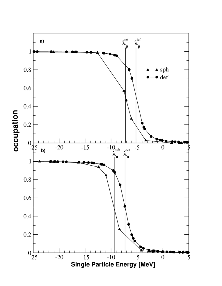
Figure 1: The proton (a) and neutron (b) occupation probabilities close to the Fermi level for ${}^{76}Se$. The spherical (sph, triangle up) and deformed (def, closed circle) BCS results correspond to pairing gaps in Eq. (32). The vertical lines denote Fermi energy for protons ($\lambda_{p}$) and neutrons ($\lambda_{n}$).

In Fig. 1 the calculated proton and neutron occupation probabilities close to the Fermi level are presented for ${}^{76}Se$. We see that both for protons and neutrons the BCS solutions associated with spherical and deformed nuclear shapes differ significantly each from other. This deformation dependence of the BCS results is expected to have strong impact on the QRPA solution.

The calculation of the QRPA energies and wave functions requires the knowledge of the particle-hole $\chi$ and particle–particle $\kappa$ strengths of the residual interaction. The optimal value of $\chi$ is determined by reproducing the systematics of the empirical position of the Gamow-Teller giant resonance in odd-odd intermediate nucleus as obtained from the $(p,n)$ reactions [47, 48]. The parameter $\kappa$ can be determined by exploiting the systematics of single $\beta$-decay feeding the initial and final nuclei. In Ref. [47] the strengths of the particle–hole and particle–particle terms of the separable Gamow-Teller force were fixed as smooth functions of mass number A by reproducing the $\beta$-decay properties of nuclei up to A=150 within the spherical pn-QRPA model. The recommended values of $\chi$ and $\kappa$ of Ref. [47] are as follows:

$$\chi=5.2/A^{0.7}~{}MeV,~{}~{}~{}~{}~{}\kappa=0.58/A^{0.7}~{}MeV.$$ (33)

In the presented $2\nu\beta\beta$-decay study of the ground state transition ${}^{76}Ge\rightarrow{{}^{76}Se}$ we use the recommended value for $\chi$ ($\chi=0.25~{}MeV$) and $\kappa$ is considered as free variable.

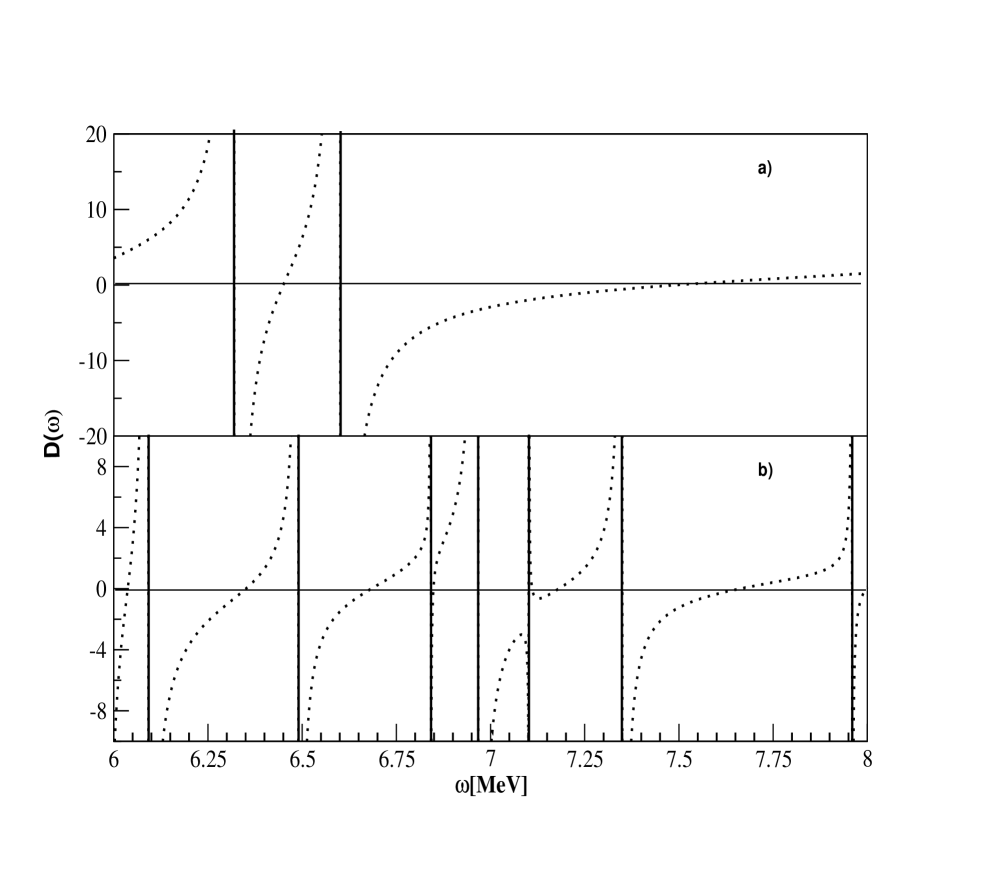
Figure 2: The l.h.s. of Eq. (16) $D(\omega)$ is plotted as function of the energy $\omega$ for ${}^{76}Ge$. The calculation has been performed within spherical (a) and deformed (b) QRPA for $\chi=0.25$ and $\kappa=0$. In case (b) the K=0 results are presented.

The QRPA calculations for the $K=0,\pm 1$ states are performed by following the procedure described in Section II. The number of zeros of the non-linear RPA secular equation in Eq. (16) is equal to the number of the two-quasiparticle configurations included in the microscopic sums (17). In the case of $K=0$ ($K=\pm 1$) the dimension of the configuration space is of the order of 450 (900) quasiparticle pairs excitations. To each zero of the RPA secular equation corresponds one RPA energy $\omega^{m}_{K}$. It is worthwhile to notice that by introducing the deformation degrees of freedom the zeros are not found in each subinterval of energy $\omega$ determined by the two subsequent two-quasiparticle excitation energies and that in some subintervals two or more zeros are found. This situation is illustrated in Fig. 2. The vertical axis is the left-hand side (l.f.s.) of Eq.(16) and the horizontal one is the energy $\omega_{K=1}$ in the range $6~{}MeV\leq\omega_{k=1}\leq 8~{}MeV$. The upper (a) and lower (b) subfigures show results for A=76 obtained within the spherical and deformed QRPA, respectively. We note that a similar phenomenon was found also in Ref. [49] in different context.

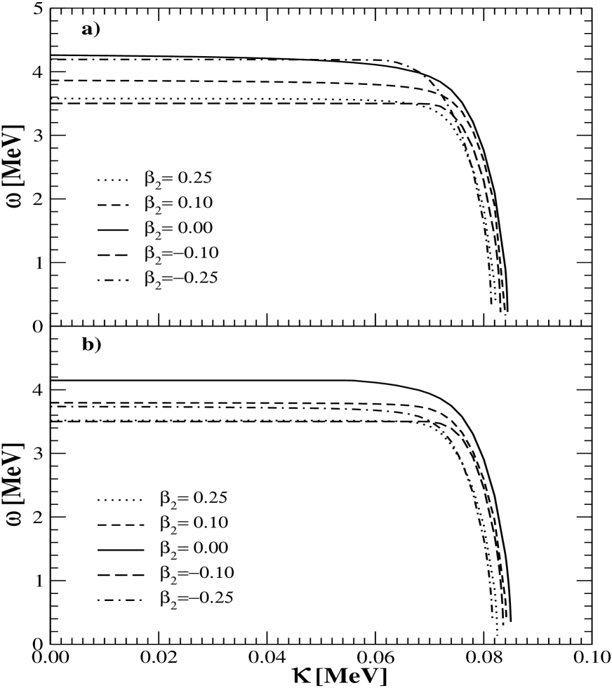
Figure 3: The energy of the lowest QRPA state as function of particle–particle interaction strength $\kappa$. The K=0 and K=1 deformed QRPA results for ${}^{76}Se$ are presented in subfigures (a) and (b), respectively.

The main drawback of the QRPA is the overestimation of the ground state correlations leading to a collapse of the QRPA ground state, which may lead to ambiguous determination of the $\beta$ and $\beta\beta$-decay matrix elements. The QRPA collapses, because it generates too many correlations with increasing strength of the attractive proton-neutron interaction as a result of the quasiboson approximation used. An interesting issue is the dependence of the position of the collapse of the QRPA solution on the deformation degrees of freedom. In Fig. 3 the energies of the lowest $K=0$ and $|K|=1$ states in ${}^{76}As$ calculated within the deformed QRPA in respect to the ${}^{76}Se$ ground state are plotted as a function of particle-particle interaction strength $\kappa$. The calculations were performed for different values of quadrupole deformation parameter $\beta_{2}$, namely $\beta_{2}=-0.25,-0.10$, $\beta_{2}=0.0$ and $\beta_{2}=0.10,0.25$ representing oblate, spherical and prolate shapes of ${}^{76}Se$, respectively. We note that in the spherical limit the energies of $K=0$ and $|K|=1$ states of the intermediate nucleus coincide to each other. Fig. 3 shows that for a deformed nucleus the collapse of the QRPA solution appears for a slightly smaller value of $\kappa$. In the case of strongly deformed ${}^{76}Se$ this effect is more pronounced in comparison with the less deformed one. Thus the deformation degrees of freedom do not improve the stability of the QRPA solution. The violation of the Pauli exclusion principle affects the QRPA results strongly in the range of particle-particle interaction $\kappa$ above $0.07$ MeV.

The half-life of the $2\nu\beta\beta$-decay of ${}^{76}Ge$ is known with high accuracy from the Heidelberg-Moscow experiment, in particular $T^{2\nu}_{1/2}=[1.55\pm 0.01(stat)^{+0.19}_{-0.15}syst.)]\times 10^{21}$ years [28]. All existing positive results on the $2\nu\beta\beta$-decay were analyzed by Barabash [9], who suggested to consider for the ground state transition ${}^{76}Ge\rightarrow{{}^{76}Se}$ the average value $T^{2\nu}_{1/2}=1.43^{+0.19}_{-0.07}\times 10^{21}$ years. By using of Eq. (27) and the knowledge of the kinematical factor $G^{2\nu}$ [$G^{2\nu}(^{76}Ge)=1.49\times 10^{-20}~{}year^{-1}~{}MeV^{2}$] from the $2\nu\beta\beta$-decay half-life of ${}^{76}Ge$ one can deduce the absolute value of the nuclear matrix element $|M_{GT}^{2\nu-exp.}|$ equal to $0.138~{}MeV^{-1}$ by assuming $g_{A}=1.25$. If the value of the axial coupling constant $g_{A}$ is considered to be unity, the value of $|M_{GT}^{2\nu-exp.}|$ deduced from the average half-life for A=76 is larger, $0.216~{}MeV^{-1}$.

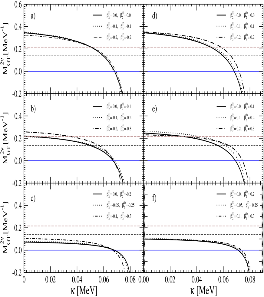
Figure 4: $2\nu\beta\beta$-decay matrix element of ${}^{76}Ge$ as function of particle–particle interaction strength $\kappa$. In the subfigures (a), (b) and (c) [(d), (e) and (f)] the results corresponding to oblate [prolate] deformation of both initial and final nuclei are presented. Please note that if the deformation of the initial and final nuclei is comparable, there is only minimal difference between the calculated values of $M^{2\nu}_{GT}$. By increasing difference in deformations of parent and daughter nuclei the suppression of $M^{2\nu}_{GT}$ is increased in the range $0~{}MeV\leq\kappa\leq 0.6~{}MeV$. The two dashed horizontal lines correspond to $M^{2\nu-exp}_{GT}=0.216~{}MeV^{-1}$ ($g_{A}=1.0$) and $M^{2\nu-exp}_{GT}=0.138~{}MeV^{-1}$ ($g_{A}=1.25$).

In Fig. 4 the effect of the deformation on the $2\nu\beta\beta$-decay matrix element $M_{GT}^{2\nu}$ is analyzed. The results for the $2\nu\beta\beta$-decay matrix element are displayed as function of the particle–particle strength $\kappa$. The curves drawn in subfigures a), b) and c) [subfigures d), e) and f)] correspond to the case both initial and final nuclei are oblate [prolate]. The two horizontal lines represent $M_{GT}^{2\nu-exp.}=0.138~{}MeV^{-1}~{}(g_{A}=1.25)$ and $M_{GT}^{2\nu-exp.}=0.216~{}MeV^{-1}~{}(g_{A}=1.0)$. By glancing Fig. 4 we note that within the whole range of $\kappa$ there is only a minimal difference between values of $M_{GT}^{2\nu}$ corresponding to the same value of $\Delta\beta_{2}$, which is defined as

$$\Delta\beta_{2}=|\beta_{2}({{}^{76}Ge})-\beta_{2}({{}^{76}Se})|.$$ (34)

In addition, one finds that by increasing the value of $\Delta\beta_{2}$ the suppression of $M_{GT}^{2\nu}$ becomes stronger within the range $0~{}MeV~{}\leq\kappa\leq 0.06~{}MeV$. This a new suppression mechanism of the $2\nu\beta\beta$-decay matrix element namely, $M_{GT}^{2\nu}$ depends strongly on difference in deformations of parent and daugter nuclei.

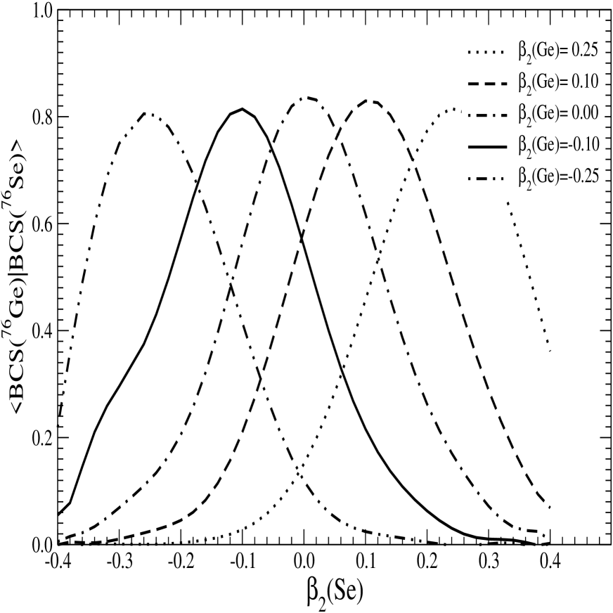
Figure 5: The overlap factor of the initial and final BCS vacua as function of the quadrupole deformation parameter $\beta_{2}$ of ${}^{76}Se$. The results are presented for spherical ($\beta_{2}=0.0$), oblate ($\beta_{2}=-0.25,-0.10$) and prolate ($\beta_{2}=0.10,0.25$) deformations of ${}^{76}Ge$.

One might ask what is the origin of this suppression. In Fig. 5 this point is clarified by presenting the overlap factor of two BCS vacua for different values of $\beta_{2}(^{76}Ge)$ as function of the quadrupole deformation of ${}^{76}Se$. We see that for a given $\beta_{2}(^{76}Ge)$ the curve has a maximum for $\beta_{2}(^{76}Se)=\beta_{2}(^{76}Ge)$ and with increasing difference in deformations of initial and final nuclei, i.e., $\Delta\beta_{2}$, the value of the BCS overlap factor decreases rapidly. From the Fig. 5 it follows that oblate-prolate (or prolate-oblate) $2\nu\beta\beta$-decay transitions are disfavoured in comparison with prolate-prolate or oblate-oblate ones for the same absolute values of associated quadrupole deformation parameters. In particular, by assuming the $\beta_{2}$ and $\beta_{4}$ parameters of Ref. [40] we obtain $<BCS(^{76}Ge)|BCS(^{76}Se)>=0.009$. This suppression is too strong to achieve agreement with experimental data for the calculated $M_{GT}^{2\nu}$. However, by changing the deformation of ${}^{76}Se$ from oblate to prolate ($\beta_{2}(^{76}Se)=0.244$) we end up with significantly larger value of the BCS overlap factor: $<BCS(^{76}Ge)|BCS(^{76}Se)>=0.61$.

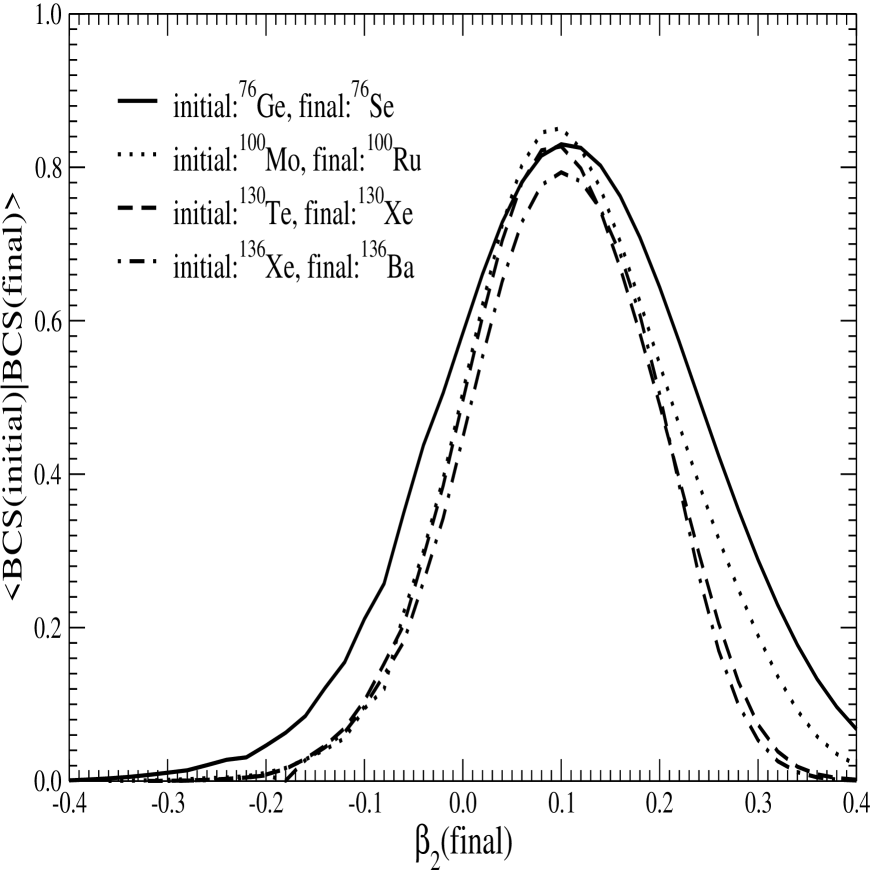
Figure 6: The overlap factor of the initial and final BCS vacua as function of the quadrupole deformation parameter $\beta_{2}$ of the final nucleus for double beta decay of ${}^{76}Ge$, ${}^{100}Mo$, ${}^{130}Te$, and ${}^{136}Xe$. The deformation parameter of the initial nucleus is chosen to be $\beta_{2}(initial)=0.1$.

The presented suppression mechanism is expecting to work also for other $2\nu\beta\beta$-decay transitions. In Fig. 6 we present BCS overlap factor for the $2\nu\beta\beta$-decay of ${}^{76}Ge$, ${}^{100}Mo$, ${}^{130}Te$ and ${}^{136}Xe$. The quadrupole deformation of the initial nucleus was taken to be $\beta_{2}=0.1$ and $\beta_{2}$ related with the final nucleus was considered to be a free parameter within the range $-0.4\leq\beta_{2}\leq 0.4$. The pairing gaps, which entered the BCS equations, are given in Eq. (32) for A=76 and for A=100, 130 and 136 are given by

$${}^{100}Mo:\Delta_{p}=1.612~{}MeV,~{}\Delta_{n}=1.358~{}MeV,~{}^{100}Ru:\Delta_{p}=1.548~{}MeV,~{}\Delta_{n}=1.296~{}MeV,$$

$${}^{130}Te:\Delta_{p}=1.043~{}MeV,~{}\Delta_{n}=1.180~{}MeV,~{}^{130}Xe:\Delta_{p}=1.299~{}MeV,~{}\Delta_{n}=1.243~{}MeV,$$

$${}^{136}Xe:\Delta_{p}=0.971~{}MeV,~{}\Delta_{n}=1.408~{}MeV,~{}^{136}Ba:\Delta_{p}=1.245~{}MeV,~{}\Delta_{n}=1.032~{}MeV.$$ (35)

We see that the behaviour of the overlap factor for all considered nuclear systems is qualitatively the same. The maximum of this factor appears for equal quadrupole deformation of the initial and final nuclei. With increasing value of $|\beta_{2}(initial)-\beta_{2}(final)|$ the value of the overlap factor strongly decreases. This fact implies that the deformation of nuclei plays an important role in the calculation of the $2\nu\beta\beta$-decay transitions and should be known with high reliability.

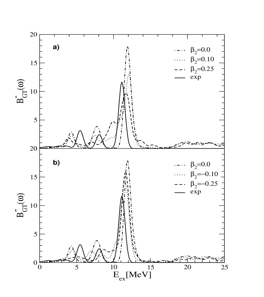
Figure 7: Gamov-Teller strength distributions $B^{-}_{GT}$ in ${}^{76}Ge$ as a function of the excitation energy of the daughter nucleus $E_{ex}$. The distributions associated with prolate and oblate deformation of ${}^{76}Ge$ are compared with that obtained for spherical shape ($\beta_{2}=0.0$) in subfigures (a) and (b), respectively. The recommended values of $\chi$ and $\kappa$ of Ref. [47] were considered: $\chi=0.25~{}MeV$ and $\kappa=0.028~{}MeV$. Experimental data (thick solid line) are from Ref. [50].

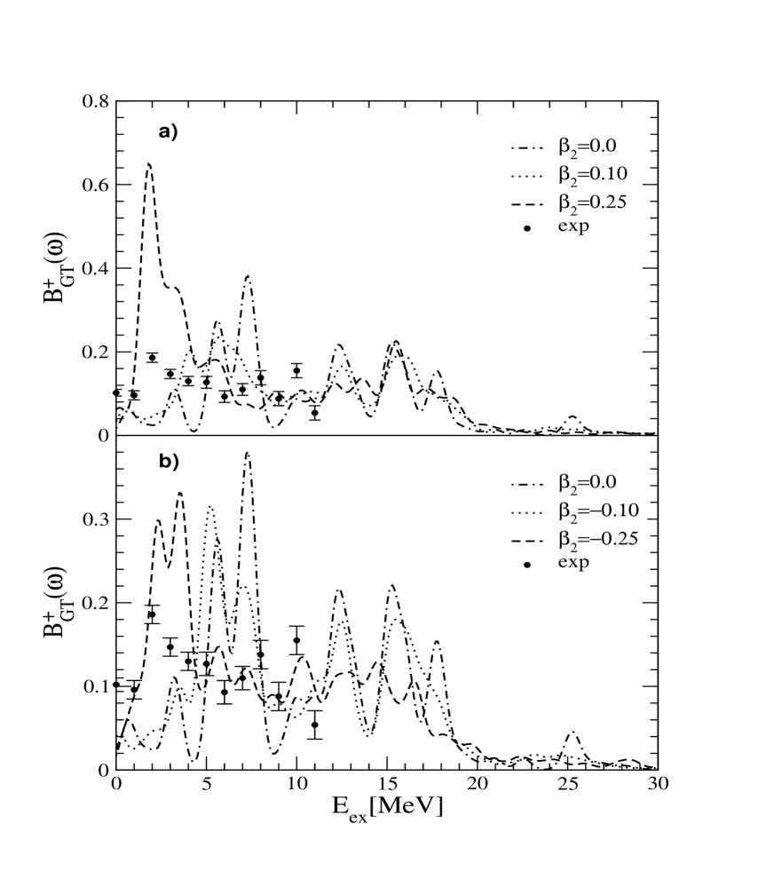
Figure 8: Gamov-Teller strength distributions $B^{+}_{GT}$ in ${}^{76}Se$ as a function of the excitation energy of the daughter nucleus $E_{ex}$. The distributions associated with prolate and oblate deformation of ${}^{76}Ge$ are compared with that obtained for spherical shape ($\beta_{2}=0.0$) in subfigures (a) and (b), respectively. It is assumed $\chi=0.25~{}MeV$ and $\kappa=0.028~{}MeV$ [47]. The data represented by the solid points are from Ref. [51].

An interesting issue is whether it is possible to obtain information about the deformations of ${}^{76}Ge$ and ${}^{76}Se$ by studying the $\beta^{-}$ and $\beta^{+}$ strength distributions in these nuclei, respectively. For different values of quadrupole parameter $\beta_{2}$ they are presented in Figs. 7 and 8. In order to facilitate comparison among various calculations the Gamow-Teller distributions are smoothed with a Gaussian of width $1~{}MeV$. The assumed strengths of the particle-hole and particle-particle interaction strength were $\chi=0.25~{}MeV$ and $\kappa=0.028~{}MeV$ [47]. By glancing at Fig. 7 we see that the position of the Gamow-Teller resonance is not sensitive to effect of deformation and that only a little strength is concentrated above the region of the Gamow-Teller resonance. However, there are significant differences between the spherical and deformed strength distributions in general [41] especially in the case of prolate shape of ${}^{76}Ge$ (see Fig. 7a), which is favoured by experimental data [44]. The thick solid line in Fig. 7 corresponds to data obtained from charge exchange ${}^{76}Ge(p,n)^{76}As$ reaction at $134.4~{}MeV$ [50], which were folded with 1 MeV width Gaussians as it has been done for the theoretical results. We see that the presented calculations are in a very good agreement with data for the position of Gamow-Teller resonance. It confirms the correct choice of the particle–hole strength of the nuclear Hamiltonian ($\chi=0.25~{}MeV$) in our calculation [47]. From Fig. 7 it also follows that the strength in the peak of the experimental $B_{GT}^{-}$ distribution is better reproduced by the QRPA calculations with only sligtly deformed mean field.

The calculated $\beta^{+}$ strength distributions in ${}^{76}Se$ are displayed in Fig. 8. They have been folded with $\Gamma=1~{}MeV$ width Gaussians. We see that the effect of deformation on the $\beta^{+}$ distribution strength for Gamow-Teller transition operator is more apparent as it is in the case $\beta^{-}$ strength distribution in ${}^{76}Ge$. In Fig. 8 we present also the experimental data, which are represented by solid points. They were obtained from charge exchange ${}^{76}Se(n,p)^{76}As$ reaction [51]. We note that the experimentally extracted strength distribution with the help of two plausible methods differ from each other by more than a factor of 2 [51]. Hence the experimental data must be considered to be of a qualitative nature only.

There are two suppression mechanisms of the $2\nu\beta\beta$-decay matrix element. Already long ago Vogel and Zirnbauer showed that $M^{2\nu}_{GT}$ is strongly suppressed when a reasonable amount of particle-particle interaction is taken into account [10], what is achieved close to a collapse of the QRPA solution. In this paper we show now that the $2\nu\beta\beta$-decay matrix element $M^{2\nu}_{GT}$ depends strongly on the difference in deformations of the initial and final nuclei. A possible criterium to decide, which deformation for the initial and the final nucleus in the double beta decay should be used could be the requirement for a common description of both single $\beta$ and $2\nu\beta\beta$-decay within the same nuclear Hamiltonian. In order to clarify this point three different cases are considered:
i) Spherical shapes of both initial and final nuclei, i.e., $\beta_{2}(^{76}Ge)=0$ and $\beta_{2}(^{76}Se)=0$.
ii) Deformations of parent and daughter nuclei: $\beta_{2}(^{76}Ge)=0.1$ and $\beta_{2}(^{76}Se)=0.266$.
iii) Quadrupole deformations of the ground state of ${}^{76}Ge$ and ${}^{76}Se$: $\beta_{2}(^{76}Ge)=0.1$ and $\beta_{2}(^{76}Se)=0.216$.
The choice of the deformation parameters in cases i) and ii) do not contradict the data [43, 44, 45].

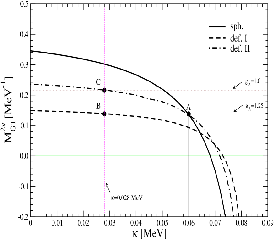
Figure 9: $2\nu\beta\beta$-decay matrix element of ${}^{76}Ge$ as function of particle–particle interaction strength $\kappa$. The solid (sph.) line corresponds to spherical shape of initial and final nuclei. The dashed (def. I) and dot-dashed (def. II) are asociated with a set of deformation parameters ($\beta_{2}(^{76}Ge)=0.1$, $\beta_{2}(^{76}Se)=0.266$) and ($\beta_{2}(^{76}Ge)=0.1$, $\beta_{2}(^{76}Se)=0.216$), respectively. The points indicated by letters A, B and C determine $\kappa$ for which the value of $M_{GT}^{2\nu-exp.}$ deduced from the $2\nu\beta\beta$-decay half-life of ${}^{76}Ge$ is obtained. For $g_{A}=1.25$ ($g_{A}=1.0$) one finds $M^{2\nu-exp}_{GT}=0.138~{}MeV^{-1}$ ($M^{2\nu-exp}_{GT}=0.216~{}MeV^{-1}$) by assuming $T^{2\nu}_{1/2}(^{76}Ge)=1.43\times 10^{21}$ years [9].

In Fig. 9 the $2\nu\beta\beta$-decay of ${}^{76}Ge$ is presented as function of particle-particle interaction strength $\kappa$ for the above three cases. In the calculation determined by case i) (spherical nuclei) $M_{GT}^{2\nu-exp.}$ equal to $0.138~{}MeV^{-1}$ ($g_{A}=1.25$) is reproduced for $\kappa=0.06~{}MeV$. The corresponding set of nuclear structure input parameters in this calculation is denoted by capital letter A (see Table 1). This value of $\kappa$ is significantly larger as the average value $\kappa_{\beta}=0.028~{}MeV$ deduced from the systematic study of the single $\beta^{+}$-decays [47]. One can hardly suppose that it is because ${}^{76}Ge$ and ${}^{76}Se$ are specific nuclear systems. They are no indications in favor of it. It seems to be a general problem within the spherical QRPA: the calculated nuclear matrix elements reproduce the experimental $2\nu\beta\beta$-decay half-lifes as a rule for particle-particle strength close to its critical value given by the QRPA collapse. In the case the calculation determined by case ii) the situation is different. $M_{GT}^{2\nu-exp.}$ is reproduced for considerable smaller value of particle-particle strength $\kappa=0.028~{}MeV$, which corresponds to that of Homa et al. [47]. The letter B donotes the coresponding set of nuclear parameters, which is listed in Table 1. If we consider the effective axial coupling constant $g_{A}=1$, used often in the nuclei, $M_{GT}^{2\nu-exp.}$ is larger, namely $0.216~{}MeV^{-1}$. Then, a smaller difference between deformations of nuclei entering $2\nu\beta\beta$-decay process is needed to reproduce this value for $\kappa\approx\kappa_{\beta}$. This is achieved with calculation of $M_{GT}$ performed within the case iii) for $\kappa=0.028~{}MeV$ (nuclear parameter set C). Nevertheless, one should keep in mind that the coupling strength of [47] has been adjusted by using of a deformed Nilsson single-particle model and $g_{A}=1.25$. Thus it is not necessarily the best possible choice. It is supposed that this prediction for $\kappa$ is more accurate for nuclei with shorter $\beta$-decay half-lifes. We note that that the curves corresponding to cases ii) and iii) do change only weakly in the range $0\leq\kappa\leq\kappa_{\beta}$. It means that the role of the particle-particle interaction within this interval is negligible.

It is worthwhile to notice that for a large value of $\kappa$ of 0.07 MeV to 0.075 the agreement with $|M_{GT}^{2\nu-exp}|$ deduced from the $2\nu\beta\beta$-decay half-life is achieved as well and that in this case the sign of $M_{GT}^{2\nu}$ is negative. However, for negative value of $M_{GT}^{2\nu}$ the correspondance with $\kappa_{\beta}$ from systematic studies of the single beta decay [47] is not achieved. Thus negative values of $M_{GT}^{2\nu}$ are disfavored due to a complete disagreement with single $\beta$-decay study of Homma et al. [47].

In what follows we shall discuss the single $\beta$ decay characteristics corresponding to three different results in Fig. 4, denoted by letters A, B and C, for which the experimental half-life of the $2\nu\beta\beta$-decay of ${}^{76}Ge$ is reproduced. The corresponding mean field and residual interaction parameters are given in Table 1.

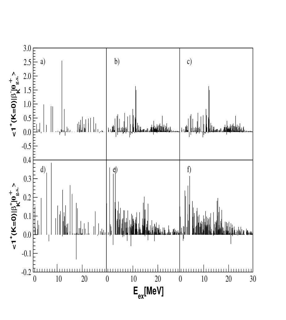
Figure 10: The $\beta^{-}$ ($\beta^{+}$) transition amplitudes between the ground state of ${}^{76}Ge$ (${}^{76}Se$) and $K=0$ intermediate states as function of the excitation energy $E_{ex}$ of ${}^{76}As$. The $\beta^{-}$ [$\beta^{+}$] results obtained for input parameter sets A, B, C (see Table 1) are presented in subfigures a) [d)], b) [e)] and c) [f)], respectively. Please observe, that the scale is different for the $\beta^{-}$ and the $\beta^{+}$ strength distributions.

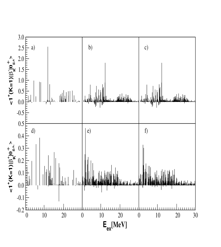
Figure 11: The same as in Fig. 10 for transitions to $K=\pm 1$ intermediate states.

The $\beta^{-}$ and $\beta^{+}$ amplitudes calculated from the ground state of ${}^{76}Ge$ and ${}^{76}Se$, respectively, associated with the $K=0$ ($K=\pm 1$) intermediate states of ${}^{76}As$ are drawn in Fig. 10 (Fig. 11). By glancing these figures we see that deformation (B and C sets of parameters) contribute to a fragmentation of the $\beta$-decay amplitudes and that values of $\beta^{+}$ amplitudes associated with higher lying states of the intermediate nucleus (up to 20 MeV) are significant. It is worthwhile to note that the absolute values of $K=0$ and $K=\pm 1$ amplitudes are equal each to other in case of the QRPA calculation with spherical mean field. The phases of these amplitudes are not of physical meaning. However, the relative phases of corresponding $\beta^{+}$ and $\beta^{-}$ amplitudes plays a crucial role due to partial destructive character of the contributions from different intermediate states to $M^{2\nu}_{GT}$. In the calculation these phases are fixed in such way that diagonal elements of the overlap matrix in Eq. (29) are taken to be positive. We note that the $K=0$ and $K=\pm 1$ contributions to $M^{2\nu}_{GT}$ differ only slightly.

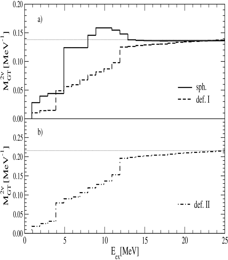
Figure 12: Running sum of the $2\nu\beta\beta$-decay matrix element $M^{2\nu}_{GT}$ as a function of the excitation energy $E_{ex}$ in ${}^{76}As$. In the upper figure (a) results corresponding to input parameter sets A (solid line) and B (dashed line) are presented. In the lower figure (b) results obtained with input parameter set C (dot-dashed line) are drawn. The dotted horizontal line in subfigure (a) [subfigure (b)] donotes the value of matrix element $M^{2\nu-exp}_{GT}=0.138~{}MeV^{-1}$ ($M^{2\nu-exp}_{GT}=0.216~{}MeV^{-1}$) deduced from the experimental $2\nu\beta\beta$-decay half-life of ${}^{76}Ge$ by assuming $g_{A}=1.25$ ($g_{A}=1.0$).

It is worthwhile to notice that a lot of $\beta^{+}$ strength in ${}^{76}Se$ is concentrated in the high energy region above $13~{}MeV$ (see Fig. 8), which can not be described within the shell model. There is a longstanding question whether in the calculation of the $2\nu\beta\beta$-decay matrix element $M^{2\nu}_{GT}$ the transitions to higher lying states of the intermediate nucleus play an important role. There is so called “Single State Dominance Hypothesis” (SSDH), which assumes that only the lowest $1^{+}$ state of the intermediate nucleus is of major importance in the evaluation of $M^{2\nu}_{GT}$. The SSDH can be realized, e.g., through cancellation among the higher lying $1^{+}$ states of the intermediate nucleus. In Ref. [52] a possibility to decide experimentally about validity of the SSDH by measuring the single electron spectra and the angular distribution of the emitted electrons was discussed. This treatment of the SSDH is suitable for the $2\nu\beta\beta$-decay transitions with low-lying $1^{+}$ ground state of the intermediate nucleus. But this is not the case of the $2\nu\beta\beta$-decay of ${}^{76}Ge$. In Fig. 12 the QRPA model dependent study of this problem is presented by drawing the running sum of matrix element $M^{2\nu}_{GT}(E)$ as a function of the $1^{+}$ excitation energy $E_{ex}$ of the intermediate nucleus. We see that in the case of the spherical calculation the main contribution to $M^{2\nu}_{GT}$ comes from the states of the intermediate nucleus lying below 5 MeV scale and that there is a partial cancellation among contributions to $M^{2\nu}_{GT}$ from higher lying states. In the case of deformed QRPA calculations there is a different situation. We see that important contributions to $M^{2\nu}_{GT}(E)$ arise even from relatively high energies of the intermediate states around the position of Gamow-Teller resonance (about 12 MeV), which can not be described for a given nuclear system in the framework of the shell model. These results contradict the SSDH and indicate that a strong truncation in consideration of the complete set of the states of the intermediate nucleus is not appropriate.

4 Summary and Conclusions

For the $2\nu\beta\beta$-decay ground state transition ${}^{76}Ge\rightarrow{{}^{76}Se}$ a detailed study of nuclear matrix elements within the deformed QRPA with separable spin–isospin interactions in the particle–hole and particle–particle channels was performed. A new mechanism of the suppression of the double beta decay nuclear matrix elements was found. We showed that the effect of deformation on the $2\nu\beta\beta$-decay matrix element is large for a significant difference in deformations of the parent and daughter nuclei and is not related with the increasing amount of the ground state correlations close to a collapse of the QRPA solution. The origin of this new mechanism is a strong sensitivity of the overlap of the initial and final BCS vacua to the deformations of the initial and final nuclei. This enters directly into the the overlap of the intermediate nuclear states generated from the initial and final nuclei via QRPA diagonalization. A study of other double beta decay transitions as a function of this deformation dependent overlap indicates the general importance of the new suppression mechanism for the $2\nu\beta\beta$-decay and $0\nu\beta\beta$-decay matrix elements.

Next, we showed that by assuming spherical nuclei there is a strong disagreement between the particle-particle strength $\kappa$ needed to reproduce the $2\nu\beta\beta$-decay half-life of ${}^{76}Ge$ and the $\kappa$ deduced in Ref. [47] from a systematic study of the single $\beta$-decay transitions. By the new suppression mechanism of the $2\nu\beta\beta$-decay matrix element we showed that for deformations of the parent and daughter nuclei, which do not contradict the experimental data, a simultaneous description of both single $\beta$ and $2\nu\beta\beta$-decay is possible. We also discussed the role of the axial coupling constant $g_{A}$.

We found that a significant part of the total $\beta^{+}$ strength is concentrated in the energy region above $10~{}MeV$. A detail study of contributions to $M^{2\nu}_{GT}$ from different $1^{+}$ intermediate nuclear states showed that for the A=76 nuclei it is necessary to consider all $1^{+}$ states of ${}^{76}As$ up to energy $15-20$ MeV. This fact disfavors theoretical studies of the $2\nu\beta\beta$-decay of medium and heavy nuclei in models with a strongly truncated basis, like the shell model.

The Gamow-Teller $\beta^{+}$ strengths and double beta decay matrix elements in medium and heavy nuclei continue to be a challenge for nuclear structure models. Further theoretical studies are needed to clarify the role of deformation in calculation of other double beta decay transitions, especially those including heavier nuclear systems, which are known to be strongly deformed. Future works should investigate the $2\nu\beta\beta$-decay matrix elements also within different possible extensions of the deformed QRPA, e.g., those including proton-neutron pairing [55]. In this way one expects to develop a reliable many-body approach with well defined nuclear structure parameters for calculation of the $0\nu\beta\beta$-decay matrix elements. Their accurate values are highly required to determine the neutrino mixing pattern and to answer the question [53] about the dominant mechanism of the $0\nu\beta\beta$-decay [54].

5 Appendix A

The single-particle states are calculated by solving the Schrödinger equation with the deformed axially symmetric Woods-Saxon potential, which parameterization is given in Ref. [36]. They are characterized by their energy $\varepsilon_{\tau}$, parity $\pi_{\tau}$ and by the projection $\Omega_{\tau}$ ($\tau=p,n$) of the full angular momentum on the nuclear symmetry axis. We use notation $|p\rho_{p}>$ and $|n\rho_{n}>$ for protons and neutrons, respectively. $|\tau\rho_{\tau}>$ represents proton ($\tau=p$) or neutron ($\tau=n$) state with quantum numbers $\Omega_{\tau}$ and $\pi_{\tau}$. $\rho_{\tau}$ is the sign of the angular momentum projection $\Omega$ ($\rho_{\tau}=\pm 1$). We note that intrinsic states are twofold degenerate. The states with $\Omega_{\tau}$ and $-\Omega_{\tau}$ have the same energy as consequence of the time reversal invariance. We shall use notation such that $\rho_{\tau}$ is taken to be positive for states and negative for time reversal states.

In order to solve the Schrödinger equation the eigenfunctions of a deformed symmetric harmonic oscillator are used as a basis for the diagonalization of the mean-field Hamiltonian [35]. These states are completely determined by a principal set of quantum numbers $(N,n_{z},\Lambda,\Omega)$, where $N=n_{x}+n_{z}$, $n_{x}=2n_{r}+|\Lambda|$ and $\Omega=\Lambda+\Sigma$. $n_{z}-1$ and $n_{x}-1$ are number of nodes of the basis functions in the $z$-direction and $r$-direction, respectively. $\Lambda$ and $\Sigma$ are the projections of the orbital and spin angular momentum on the symmetry axis z. The explicit form of single-particle harmonic oscillator wave functions in cylindrical coordinates $(r,z,\phi)$ can be found, e.g., in Ref. [37]. For a given shape of the nuclear surface, the shape of the deformed harmonic oscillator is automatically chosen in a way suitable for obtaining good accuracy with a smallest number of basis functions [35]. The deformation dependent cutt-off is chosen in such way as to assure numerical stability of the results. In our calculation we use 11 major shells.

In cylindrical coordinates the eigenfunctions of states and time-reversed states in deformed Woods-Saxon potential are expressed as follows:

$$|\tau\rho_{\tau}=+1> = \sum_{Nn_{z}}[b^{(+)}_{Nn_{z}\Omega_{\tau}}|N,n_{z},\Lambda_{\tau},\Omega_{\tau}=\Lambda_{\tau}+1/2>+$$ (36)

$$~{}~{}~{}~{}~{}b^{(-)}_{Nn_{z}\Omega_{\tau}}|N,n_{z},\Lambda_{\tau}+1,\Omega_{\tau}=\Lambda_{\tau}+1-1/2>]$$

and

$$|\tilde{\tau}\rho_{\tau}=+1> = |\tau\rho_{\tau}=-1>=\sum_{Nn_{z}}[b^{(+)}_{Nn_{z}\Omega_{\tau}}|N,n_{z},-\Lambda_{\tau},\Omega=-\Lambda_{\tau}-1/2>-$$ (37)

$$~{}~{}~{}~{}~{}b^{(-)}_{Nn_{z}\Omega_{\tau}}|N,n_{z},-\Lambda_{\tau}-1,\Omega_{\tau}=-\Lambda_{\tau}-1+1/2>]$$

with $\Lambda\geq 0$. $\sim$ indicates time reversal states.

The single-particle matrix elements of the $\tau^{+}\sigma_{K}$ operator are given by

$$<p\rho_{p}|\tau^{+}\sigma_{K=0}|n\rho_{n}> = \delta_{\Omega_{p}\Omega_{n}}\rho_{p}\sum_{Nn_{z}}[b^{(+)}_{Nn_{z}\Omega_{p}}b^{(+)}_{Nn_{z}\Omega_{n}}-b^{(-)}_{Nn_{z}\Omega_{p}}b^{(-)}_{Nn_{z}\Omega_{n}}],$$ (38)

$$<p\rho_{p}|\tau^{+}\sigma_{K=+1}|n\rho_{n}> = -\sqrt{2}\delta_{\Omega_{p}\Omega_{n}+1}\sum_{Nn_{z}}b^{(+)}_{Nn_{z}\Omega_{p}}b^{(-)}_{Nn_{z}\Omega_{n}}~{}~{}~{}for~{}~{}\rho_{p}=\rho_{n}=+1,$$ (39)

$$= +\sqrt{2}\delta_{\Omega_{p}\Omega_{n}+1}\sum_{Nn_{z}}b^{(-)}_{Nn_{z}\Omega_{p}}b^{(+)}_{Nn_{z}\Omega_{n}}~{}~{}~{}for~{}~{}\rho_{p}=\rho_{n}=-1,$$

$$= -\sqrt{2}\delta_{\Omega_{p}\frac{1}{2}}\delta_{\Omega_{n}-\frac{1}{2}}\sum_{Nn_{z}}b^{(+)}_{Nn_{z}\Omega_{p}}b^{(+)}_{Nn_{z}\Omega_{n}}~{}~{}~{}for~{}~{}\rho_{p}=+1,~{}\rho_{n}=-1,$$

$$<p\rho_{p}|\tau^{+}\sigma_{K=-1}|n\rho_{n}> = \sqrt{2}\delta_{\Omega_{p}\Omega_{n}-1}\sum_{Nn_{z}}b^{(-)}_{Nn_{z}\Omega_{p}}b^{(+)}_{Nn_{z}\Omega_{n}}~{}~{}~{}for~{}~{}\rho_{p}=\rho_{n}=+1,$$ (40)

$$= -\sqrt{2}\delta_{\Omega_{p}\Omega_{n}-1}\sum_{Nn_{z}}b^{(+)}_{Nn_{z}\Omega_{p}}b^{(-)}_{Nn_{z}\Omega_{n}}~{}~{}~{}for~{}~{}\rho_{p}=\rho_{n}=-1,$$

$$= \sqrt{2}\delta_{\Omega_{p}-\frac{1}{2}}\delta_{\Omega_{n}\frac{1}{2}}\sum_{Nn_{z}}b^{(+)}_{Nn_{z}\Omega_{p}}b^{(+)}_{Nn_{z}\Omega_{n}}~{}~{}~{}for~{}~{}\rho_{p}=+1,~{}\rho_{n}=-1.$$

The overlap of the proton and neutron single particle states of the initial $(A,Z)$ and final $(A,Z+2)$ nuclei are calculated by assuming that the corresponding sets of basis wave functions do not differ significantly each from other. Then we have

$$<p_{f}\rho_{p_{f}}|p_{i}\rho_{p_{i}}> = \delta_{\Omega_{p_{f}}\Omega_{p_{i}}}\sum_{Nn_{z}}[b^{(+)}_{Nn_{z}\Omega_{p_{f}}}b^{(+)}_{Nn_{z}\Omega_{p_{i}}}-b^{(-)}_{Nn_{z}\Omega_{p_{f}}}b^{(-)}_{Nn_{z}\Omega_{p_{i}}}],$$

$$<n_{f}\rho_{n_{f}}|n_{i}\rho_{n_{i}}> = \delta_{\Omega_{n_{f}}\Omega_{n_{i}}}\sum_{Nn_{z}}[b^{(+)}_{Nn_{z}\Omega_{n_{f}}}b^{(+)}_{Nn_{z}\Omega_{n_{i}}}-b^{(-)}_{Nn_{z}\Omega_{n_{f}}}b^{(-)}_{Nn_{z}\Omega_{n_{i}}}].$$ (41)

The index i (f) denotes that proton and neutron single particle states are defined with respect to the initial (final) nucleus.

6 Appendix B

As a consequence of considered many-body approximations the two sets of intermediate nuclear states generated from the initial and final ground states are not identical within the QRPA theory. Thus it is necessary to introduce the overlap factor of these states, which can be expressed with the help of intrinsic phonon operators as follows:

$$<1(K),m_{f}|1(K),m_{i}>=<rpa_{f}|~{}Q^{m_{f}}_{K}~{}{Q^{m_{i}\dagger}_{K}}~{}|rpa_{i}>.$$ (42)

Here, the index i (f) indicates that the excited states of the nucleus are defined with respect to the initial (final) nuclear ground state $|rpa_{i}>$ ($|rpa_{f}>$).

In order to evaluate $<1(K),m_{f}|1(K),m_{i}>$ we express the phonon creation operator ${Q^{m_{i}}_{K}}^{\dagger}$ in terms of creation and anninhilation phonon operators associated with the final nucleus. We have

$${Q^{m_{i}\dagger}_{K}}=\sum_{m_{f}}~{}(a_{m_{i}m_{f}}{Q^{m_{f}\dagger}_{K}}~{}+~{}b_{m_{i}m_{f}}{\tilde{Q}}^{m_{f}}_{K}).$$ (43)

The coefficients of expansion $a_{m_{i}m_{f}}$ and $b_{m_{i}m_{f}}$ will be determined below. By inserting Eq. (43) into Eq. (42) we get

$$<1(K),m_{f}|1(K),m_{i}> = \sum_{{m^{\prime}}_{f}}[<rpa_{f}|Q^{m_{f}}_{K}{Q^{{m^{\prime}}_{f}\dagger}_{K}}|rpa_{i}>a_{m_{i}{m^{\prime}}_{f}}$$ (44)

$$+<rpa_{f}|Q^{m_{f}}_{K}{Q^{{m^{\prime}}_{f}}_{-K}}|rpa_{i}>b_{m_{i}{m^{\prime}}_{f}}]$$

$$\approx a_{m_{i}{m^{\prime}}_{f}}<BCS_{f}|BCS_{i}>.$$

Here, we neglected overlap matrix element between the final ground state and the two-phonon state generated from the initial nucleus, which is considered to be small and should be not related with the studied quantity. In addition, we approximated the overlap of initial and final RPA ground state with the BCS ones. Thus the overlap factor of the intermediate nuclear states generated from the initial and final ground states is proportional to the overlap of initial and final BCS vacua.

We proceed with the calculation of $a_{m_{i}{m^{\prime}}_{f}}$ and $b_{m_{i}{m^{\prime}}_{f}}$ coefficients. The quasiparticle creation and anninhilation operators $(a^{(i)\dagger},a^{(i)})$ [$(a^{(f)\dagger},a^{(f)})$] of the initial [final] nucleus are connected with the particle creation and annihilation operators $(c^{(i)\dagger},c^{(i)})$ [$(c^{(f)\dagger},c^{(f)})$] by the BCS transformation [see Eq. (4)]. In addition there is a unitary transformation between particle operators associated with initial and final nuclei

$${c^{(i)\dagger}_{\tau\rho_{\tau}}} = \sum_{\tau^{\prime}{\rho}_{\tau^{\prime}}}<\tau\rho_{\tau}|\tau^{\prime}{\rho}_{\tau^{\prime}}>{c^{(f)\dagger}_{\tau^{\prime}{{\rho}_{\tau^{\prime}}}}}$$

$${{\tilde{c}}^{(i)}_{\tau\rho_{\tau}}} = \sum_{\tau^{\prime}{\rho}_{\tau^{\prime}}}<\tau\rho_{\tau}|\tau^{\prime}{\rho}_{\tau^{\prime}}>{{\tilde{c}}^{(f)}_{\tau^{\prime}{{\rho}_{\tau^{\prime}}}}}$$ (45)

The overlap factors of the single particle wave functions of the initial and final nuclei $<\tau\rho_{\tau}|\tau^{\prime}{\rho^{\prime}}_{\tau^{\prime}}>$ is given explicitely in the Appendix A. The above mentioned transformations allow us, by using the quasiboson approximation, to rewrite the boson operators of the initial nucleus with the help of the boson operators of the final nucleus:

$$A^{(i)\dagger}(l,K) = \sum_{l^{\prime}}[{\cal R}_{ll^{\prime}}A^{(f)\dagger}(l^{\prime},K)+{\cal S}_{ll^{\prime}}A^{(f)}({\overline{l}}^{\prime},K)],$$

$$A^{(i)}({\overline{l}},K) = \sum_{l^{\prime}}[{\cal R}_{ll^{\prime}}A^{(f)}({\overline{l}}^{\prime},K)-{\cal S}_{ll^{\prime}}A^{(f)\dagger}({l}^{\prime},K)].$$ (46)

Assuming the definition of the quasiparticle pairs operator in Eq. (11) the factors ${\cal R}_{ll^{\prime}}$ and ${\cal S}_{ll^{\prime}}$ can be expressed as

$${\cal R}_{ll^{\prime}} = <p\rho_{p}|p^{\prime}{\rho}_{p^{\prime}}>(u^{(i)}_{p}u^{(f)}_{p^{\prime}}+v^{(i)}_{p}v^{(f)}_{p^{\prime}})<n\rho_{n}|n^{\prime}{\rho}_{n^{\prime}}>(u^{(i)}_{n}u^{(f)}_{n^{\prime}}+v^{(i)}_{n}v^{(f)}_{n^{\prime}}),$$

$${\cal S}_{ll^{\prime}} = <p\rho_{p}|p^{\prime}{\rho}_{p^{\prime}}>(u^{(i)}_{p}v^{(f)}_{p^{\prime}}-u^{(i)}_{p}v^{(f)}_{p^{\prime}})<n\rho_{n}|n^{\prime}{\rho}_{n^{\prime}}>(u^{(i)}_{n}v^{(f)}_{n^{\prime}}-u^{(i)}_{n}v^{(f)}_{n^{\prime}}).$$ (47)

It is worthwhile to notice that in the limit initial and final states are indentical ${\cal R}_{ll^{\prime}}=1$ and ${\cal S}_{ll^{\prime}}=0$.

By inserting Eq. (46) into the expression for the phonon operator of the initial nucleus [see Eq. (13)] and by exploiting the relations

$$A^{(f)\dagger}(l,K) = \sum_{m_{f}}[X^{m_{f}}_{i,K}{Q^{m_{f}\dagger}_{K}}+Y^{m}_{i,K}{{\tilde{Q}}^{m}_{K}}],$$

$$A^{(f)}({\overline{l}},K) = \sum_{m_{f}}[X^{m_{f}}_{i,K}{{\tilde{Q}}^{m_{f}}_{K}}+Y^{m_{f}}_{i,K}{{Q}^{m_{f}\dagger}_{K}}],$$ (48)

we find [31]

$$a_{m_{i}m_{f}} = \sum_{ll^{\prime}}[X^{m_{f}}_{l^{\prime}K}{\cal R}_{l^{\prime}l}X^{m_{i}}_{lK}-Y^{m_{f}}_{l^{\prime}K}{\cal R}_{l^{\prime}l}Y^{m_{i}}_{lK}$$ (49)

$$~{}+~{}Y^{m_{f}}_{l^{\prime}K}{\cal S}_{l^{\prime}l}X^{m_{i}}_{lK}-Y^{m_{f}}_{l^{\prime}K}{\cal S}_{l^{\prime}l}Y^{m_{i}}_{lK}].$$

By neglecting the terms proportional to ${\cal S}_{ll^{\prime}}$ due to their smallness we end up with the overlap factor of the intermediate nuclear states given in Eq. (29).

The overlap factor of the initial and final BCS vacua can be written as product of proton and neutron BCS overlap factors for a given anular momentum projection quantum number $\Omega$:

$$<BCS_{f}|BCS_{i}> = <BCS_{f}(p)|BCS_{i}(p)><BCS_{f}(n)|BCS_{i}(n)>$$ (50)

$$= \prod_{\Omega_{p}}<BCS_{f}(\Omega_{p})|BCS_{i}(\Omega_{p})>\prod_{\Omega_{n}}<BCS_{f}(\Omega_{n})|BCS_{i}(\Omega_{n})>.$$

where

$$<BCS_{f}(\Omega)|BCS_{i}(\Omega)>~{}=~{}<|\prod_{k=1}^{N_{\Omega}}\left(u^{(f)}_{k}+v^{(f)}_{k}c^{(f)}_{\overline{k}}c^{(f)}_{k}\right)~{}\prod_{l=1}^{N_{\Omega}}\left(u^{(i)}_{l}+v^{(i)}_{l}c^{(i)\dagger}_{l}c^{(i)\dagger}_{\overline{l}}\right)|>.$$ (51)

$N_{\Omega}$ is the number of single particle states with the same value of quantum number $\Omega$. The same model space for protons and neutrons is assumed. By a direct calculation of the above matrix element one finds

$$<BCS_{f}(\Omega)|BCS_{i}(\Omega)>=\prod_{k=1}^{N_{\Omega}}u^{(f)}_{k}~{}\prod_{l=1}^{N_{\Omega}}u^{(f)}_{l}$$ (52)

$$+ \sum_{m_{1},n_{1}=1}^{N_{\Omega}}~{}v^{(f)}_{{m_{1}}}~{}v^{(i)}_{{n_{1}}}~{}\left(D^{(1)}(m_{1};n_{1})\right)^{2}~{}\prod_{k=1}^{N_{\Omega}(m_{1})}u^{(f)}_{k}~{}\prod_{l=1}^{N_{\Omega}(n_{1})}u^{(i)}_{l}$$

$$+ \sum_{m_{1},m_{2},n_{1},n_{2}=1}^{N_{\Omega}}~{}v^{(f)}_{{m_{1}}}v^{(f)}_{{m_{2}}}~{}v^{(i)}_{{n_{1}}}v^{(i)}_{{n_{2}}}\left(D^{(2)}(m_{1},m_{2};n_{1},n_{2})\right)^{2}~{}\prod_{k=1}^{N_{\Omega}(m_{1},m_{2})}u^{(f)}_{k}~{}\prod_{l=1}^{N_{\Omega}(n_{1},n_{2})}u^{(i)}_{l}$$

$$+ ~{}\cdot\cdot\cdot~{}+~{}\left(D^{(N_{\Omega})}(1,2,...,N_{\Omega};1,2,..,N_{\Omega})\right)^{2}~{}\prod_{k=1}^{N_{\Omega}}v^{(f)}_{{k}}~{}\prod_{l=1}^{N_{\Omega}}v^{(i)}_{{l}}.$$

Here, $\prod_{k=1}^{N_{\Omega}(m_{1},m_{2})}$ means that index $k$ runs the values from 1 to $N_{\Omega}$ except the values $k=m_{1}$ and $k=m_{2}$ ($1\leq m_{1}\leq N_{\Omega}$ and $1\leq m_{2}\leq N_{\Omega}$). $D^{r}(m_{1},m_{2},...,m_{r};n_{1},n_{2},...,n_{r})$ denotes the determinant of matrix of rank $r$ constructed of elements of the unitary matrix of the transformation between the initial and final single particle states with row indices $m_{1},m_{2},...,m_{r}$ and column indices $n_{1},n_{2},...,n_{r}$. It is worthwhile to notice that by replacing all determinants in Eq. (52) with unity, i.e. the matrix of the transformation between the single particles associated with both nuclei is just unity matrix, we obtain a compact expression [20]

$$<BCS_{f}(\Omega)|BCS_{i}(\Omega)>=\prod_{k=1}^{N_{\Omega}}(u^{(f)}_{k}u^{(i)}_{k}+v^{(f)}_{k}v^{(i)}_{k}).$$ (53)

However, this approximation is not justified and can lead to a significant inaccuracy in the calculation of $M_{GT}^{2\nu}$ especially if there is a strong difference in deformations of the intial and final nuclei.

7 Acknowledgements

We are thankful to A.A. Raduta and P. Sarriguren for stimulating comments and discussions. This work was supported in part by the Deutsche Forschungsgemeinschaft (436 SLK 17/298), by the “Land Baden-Würtemberg” as a “Landesforschungsschwerpunkt: Low Energy Neutrinos” and by the VEGA Grant agency of the Slovac Republic under contract No. 1/0249/03.

Table 1: Three sets of nuclear structure input parameters (A, B, and C) for which the calculated nuclear matrix elements $M^{2\nu}_{GT}$ reproduces the experimental $2\nu\beta\beta$-decay half-life of ${}^{76}Ge$. v.o.f. denotes overlap factor of the initial and final BCS vacua.

	mean field of ${}^{76}Ge$				mean field of ${}^{76}Se$
	Def.	Pairing			Def.	Pairing			$H_{int}$
par.	$\beta_{2}$	$\Delta_{p}$	$\Delta_{n}$		$\beta_{2}$	$\Delta_{p}$	$\Delta_{n}$	v.o.f.	$\chi$	$\kappa$	$g_{A}$	$M^{2\nu}_{GT}$
set		$MeV$	$MeV$			$MeV$	$MeV$		$MeV$	$MeV$		$MeV^{-1}$
A	0.0	1.561	1.535		0.0	1.751	1.710	0.842	0.25	0.060	1.25	0.138
B	0.10	1.561	1.535		0.266	1.751	1.710	0.403	0.25	0.028	1.25	0.138
C	0.10	1.561	1.535		0.216	1.751	1.710	0.587	0.25	0.028	1.00	0.216

References

- [1] Amand Faessler and F. Šimkovic, J. Phys. G 24 (1998) 2139.
- [2] J. Suhonen, O. Civitarese, Phys. Rep. 300 (1998) 2139.
- [3] H. Ejiri, Phys. Rep. 338 (2000) 265.
- [4] M. Doi, T. Kotani and E. Takasugi, Prog. Theor. Phys., Suppl. 83 (1985) 1.
- [5] H.V. Klapdor-Kleingrothaus, Springer Tracts in Modern Physics, Vol. 163 (Springer-Verlag, 2000), pp. 69-104.
- [6] S.R. Elliott and P. Vogel, Ann. Rev. Nucl. Part. Sci. 52 (2002) 115.
- [7] J.D. Vergados, Phys. Rep. 361 (2002) 1.
- [8] V.I. Tretyak and Yu.G. Zdesenko, At. Data Nucl. Data Tabl. 80 (2002) 83.
- [9] A.S. Barabash, Czech. J. Phys. 52 (2002) 567.
- [10] P. Vogel and M. R. Zirnbauer, Phys. Rev. Lett. 57 (1986) 3148.
- [11] O. Civitarese, A. Faessler and T. Tomoda, Phys. Lett. B 194 (1986) 11.
- [12] K. Muto, E. Bender and H. V. Klapdor, Z. Phys. A 334 (1989) 177.
- [13] M.K. Cheoun, A. Bobyk, Amand Faessler F. Šimkovic and G. Teneva, Nucl. Phys. A 561 (1993) 74; Nucl. Phys. A 564 (1993) 329.
- [14] J. Toivanen, J. Suhonen, Phys. Rev. Lett. 75 (1995) 410.
- [15] J. Schwieger, F. Šimkovic, and A. Faessler, Nucl. Phys. A 600 (1996) 179.
- [16] A.A. Raduta, A. Faessler, S. Stoica, and W.A. Kaminski, Phys. Lett. B 254 (1991) 7; Nucl. Phys. A 534 (1991) 149.
- [17] A. A. Raduta, F. Šimkovic, A. Faessler, J. Phys. G 26 (2000) 793.
- [18] L. Zamick and N. Auerbach, Phys. Rev. C 26 (1982) 2185.
- [19] D. Bogdan, A. Faessler, A. Petrovici, and S. Holan, Phys. Lett. B 150 (1985) 29.
- [20] K. Grotz and H.V. Klapdor, Phys. Lett. B 157 (1985) 242.
- [21] J.G. Hirsch, O. Castanos, P.E. Hess, Rev. Mex. Fis. 38 Suppl. 2 (1992) 66; O. Castanos, J.G. Hirsch, P.E. Hess, Rev. Mex. Fis. 39 Suppl. 2 (1993) 29.
- [22] O. Castanas, J.G. Hirsch, O. Civitarese, and P.O. Hess, Nucl. Phys. A 571 (1994) 276; J.G. Hirsch, O. Castanas, P.E. Hess and O. Civitarese, Nucl. Phys. A 589 (1995) 445; Phys. Rev. C 51 (1995) 2252.
- [23] A.A. Raduta, A. Faessler, D.S. Delion, Phys. Lett. B 312 (1993) 13, Nucl. Phys. A 564 (1993) 185.
- [24] B.M. Dixit, P.K. Rath, and P.K. Raina, Phys. Rev. C 65 (2002) 034311.
- [25] J. Krumlinde and P. Möller, Nucl. Phys. A 417 (1984) 447.
- [26] P. Sarriguren, E.Moya de Guerra, A. Escuderos, A.C. Carrizo, Nucl. Phys. A 635 (1998) 55.
- [27] P. Sarriguren, E. Moya de Guerra, A. Escuderos, Nucl. Phys. A 658 (1999) 13; Phys. Rev. C 64 (2001) 064306; Nucl. Phys. A 691 (2001) 631.
- [28] H.V. Klapdor-Kleingrothaus et al., Eur. Phys. J. A 12 (2001) 147.
- [29] Yu. Zdesenko, Rev. Mod. Phys. 74 (2002) 663.
- [30] W.C. Haxton and G.S. Stephenson, Prog. Part. Nucl. Phys. 12 (1984) 409.
- [31] F. Šimkovic, G. Pantis, A. Faessler, Prog. Part. Nucl. Phys. 40 (1998) 285; Phys. Atom. Nucl. 61 (1998) 1218.
- [32] W.A. Kaminski and A. Faessler, Nucl. Phys. A 529 (1991) 605.
- [33] J. Suhonen, Phys. Lett. B 477 (2000) 99.
- [34] A. Griffiths and P. Vogel, Phys. Rev. C 46 (1992) 181.
- [35] J. Damgaard, H.C. Pauli, V.V. Pashkevich, and V.M. Strutinski, Nucl. Phys. A 135 (1969) 432.
- [36] Y. Tanaka, Y. Oda, F. Petrovich, and R.K. Sheline, Phys. Lett. B 83 (1979) 279.
- [37] R. Nojarov, Z. Bochnacki, and A. Faessler, Z. Phys. A 324 (1986) 289.
- [38] R. Nojarov, A. Faessler, P. Sarriguren, E. Moya de Guerra and M. Grigorescu, Nucl. Phys. A 563 (1993) 349.
- [39] P. Sarriguren, E. Moya de Guerra, R. Nojarov and A. Faessler, J. Phys. G 19 (1993) 291; G 20 (1994) 315.
- [40] G.A. Lalazissis, S. Raman, P. Ring, At. Data Nucl. Data Tabl. 71 (1999) 1.
- [41] P. Sarriguren, E. Moya de Guerra, L. Pacearescu, A. Faessler, F. Šimkovic and A.A. Raduta, Phys. Rev. C 67 (2003) 044313.
- [42] P. Möller, J.R. Nix, W.D. Myers and W.J. Swiatecki, At. Data Nucl. Data Tabl. 59 (1995) 185.
- [43] S. Balraj, Nucl. Data Sheets 74 (1995) 63.
- [44] P. Raghavan, At. Data Nucl. Data Tabl. 42 (1989) 189; N.J. Stone, Oxford University preprint, http://ie.lbl.gov/toi.html.
- [45] S. Raman, C.H. Malarkey, W.T. Milner, C.W. Nestor Jr. and P.H. Stelson, At. Data Nucl. Data Tabl. 36 (1987) 1.
- [46] G. Audi and A.H. Wapstra, Nucl. Phys. A 595 (1995) 409; G. Audi, O. Bersillon, J. Blachot, and A.H. Wapstra, Nucl. Phys. A 624 (1997) 1.
- [47] H. Homma, E. Bender, M. Hirsch, K. Muto, H.V. Klapdor–Kleingrothaus, and T. Oda, Phys. Rev. C 54 (1996) 2972.
- [48] J. Suhonen, J. Taigel, and A. Faessler, Nucl. Phys. A 486 (1988) 91.
- [49] A.A. Raduta, V. Ceausescu, A. Gheorghe, and M. Popa, Nucl. Phys. A 427 (1984) 1.
- [50] R. Madey, B.S. Flanders, B.D. Anderson, A.R. Baldwin, J.W. Watson, S.M. Austin, C.C. Foster, H.V. Klapdor and K. Grotz, Phys. Rev. C 40 (1989) 540.
- [51] R.L. Helmer et al., Phys. Rev. C 55 (1997) 2802.
- [52] F. Šimkovic, P. Domin, S.V. Semenov, J. Phys. G 27 (2001) 2233.
- [53] S.M. Bilenky, C. Giunti, W. Grimus, B. Kayser, and S.T. Petcov, Phys. Lett. B 465 (1999) 193; H.V. Klapdor-Kleingrothaus, H. Päs, A.Y. Smirnov, Phys. Rev. D 63 (2001) 073005.
- [54] A. Faessler and F. Šimkovic, Prog. Part. Nucl. Phys. 48 (2001) 233.
- [55] F. Šimkovic, Ch. Moustakidis, L. Pacearescu and A. Faessler, submitted to Phys. Rev. C