Abstract

A new version of the method of Continuum-Discretized Coupled-Channels method (CDCC) is proposed, that is, the Eikonal-CDCC method (E-CDCC). The E-CDCC equation, for Coulomb dissociation in particular, can easily and safely be solved, since it is a first-order differential equation and contains no huge angular momentum in contrast to the CDCC one. The scattering amplitude calculated by E-CDCC has a similar form to that by CDCC. Then one can construct hybrid amplitude in an intuitive way, i.e., CDCC amplitude is adopted for a smaller angular momentum $L$ and E-CDCC one for a larger $L$ related to an impact parameter $b$. The hybrid calculation is found to perfectly reproduce the quantum mechanical result for ⁵⁸Ni(⁸B,⁷Be$+p$)⁵⁸Ni at 240 MeV, which shows its applicability to systematic analysis of ⁸B dissociation to extract the astrophysical factor $S_{17}$ with high accuracy.

1 Introduction

The solar neutrino problem is one of the central issues in the neutrino physics [1]. Nowadays, the neutrino oscillation is assumed to be the solution of the problem and the solar neutrino physics moves its focus on determining oscillation parameters: the mass difference among $\nu_{e}$, $\nu_{\mu}$ and $\nu_{\tau}$, and their mixing angles [2]. The astrophysical factor $S_{17}$, defined by $S_{17}(E)\equiv\sigma_{p\gamma}(E)E\exp[2\pi\eta]$ with $\sigma_{p\gamma}$ the cross section of the $p$-capture reaction ⁷Be($p,\gamma$)⁸B and $\eta$ the Sommerfeld parameter, plays an essential role in the parameter-search procedure, since the prediction value for the flux of ⁸B neutrino, which is intensively being detected on the earth, is proportional to $S_{17}(0)$. The required accuracy from astrophysics is about 5% in errors.

Because of difficulties of direct measurements for the $p$-capture reaction at very low energies, alternative indirect measurements were proposed. $p$-transfer reaction [3, 4, 5] with the Asymptotic Normalization Coefficient (ANC) method [6] and ⁸B Coulomb dissociation [7, 8, 9] are typical examples of them; we concentrate on the latter in the present paper. ⁸B Coulomb dissociation can be assumed to be the inverse reaction of ⁷Be($p,\gamma$)⁸B provided the ⁸B is dissociated through only its E1 transition by absorption of virtual photons. Once this condition is satisfied, cross section of the $p$-capture reaction, thus $S_{17}(E)$, can easily be obtained by applying the principle of detailed balance to the measured dissociation cross sections. Intensive measurements of the ⁸B Coulomb dissociation are being made in RIKEN [7], GSI [8] and MSU [9]; the extracted $S_{17}(0)$ are almost consistent each others. There is, however, contradiction between MSU and RIKEN data about the contribution of the E2 component. Additionally, role of nuclear interaction, interference between nuclear and Coulomb interactions in particular, has not yet clarified quantitatively. Therefore, it can be said that the extracted $S_{17}(0)$ from those ⁸B Coulomb dissociation measurements contain uncertainties to some extent.

In order to determine $S_{17}(0)$ accurately, careful analysis of the ⁸B dissociation including both nuclear and Coulomb interactions is necessary. The method of Continuum-Discretized Coupled-Channels (CDCC) [10], which was proposed and developed by Kyushu group, is suitable for that purpose. In fact, it was shown in Ref. [9] that CDCC can very well reproduce the MSU data. It is not straightforward, however, to extract the component corresponding to the inverse reaction of ⁷Be($p,\gamma$)⁸B out of the total measured spectra.

Very recently [11], we proposed a procedure that determines $S_{17}(0)$ from the ⁸B dissociation measurements by using the ANC method, which is free from uncertainties by the use of the detailed balance. An important advantage of the CDCC + ANC analysis is that one can quantitatively evaluate the accuracy of the extracted $S_{17}(0)$; the fluctuation of ANC by changing the ⁸B single particle wave functions is interpreted as the error of $S_{17}(0)$ coming from the use of the ANC method. We analyzed ⁵⁸Ni(⁸B,⁷Be$+p$)⁵⁸Ni at 25.8 MeV measured at Notre Dame [12], for which detailed balance was found to fail to obtain $S_{17}(0)$ because of its low incident energy [13]. The extracted $S_{17}(0)$ is 22.83 $\pm$ 0.51 (theo) $\pm$ 2.28 (expt) eVb and the ANC method turned out to work very well, i.e., less than 1% of error; the remaining theoretical error comes from the choice of the modelspace of CDCC calculation. Although quite large systematic error (10%) of the experimental data prevents one from determining $S_{17}(0)$ with the required accuracy, this method significantly reduces theoretical errors of $S_{17}(0)$.

The CDCC + ANC analysis is expected to be applicable to the RIKEN and MSU data at several tens of MeV/nucleon. From practical point of view, however, CDCC calculation including long-ranged Coulomb coupling-potentials requires extremely large modelspace rather difficult to handle; typically the required number of partial waves is 15,000 for the MSU data [9]. Although interpolation technique for angular momentum reduces the number of Coupled-Channels (CC) equations to be solved, CC equation with huge angular momentum $L$ is rather unstable and careful treatment is necessary. In this sense, it seems almost impossible to apply CDCC to the GSI data at 250 MeV/nucleon, where more than 100,000 partial waves will be required.

In the present paper we propose a new version of CDCC; the Eikonal-CDCC method (E-CDCC) being based on eikonal and non-adiabatic calculation. Since E-CDCC equations contain no angular momentum for the relative motion of a projectile and a target nucleus, the $S$ matrix is obtained easily and safely. Another important feature of the method is that the resultant scattering amplitude has the form which is very similar to that obtained by CDCC, by using the relation between impact parameter $b$ and $L$. This allows one hybrid calculation, i.e., one can adopt the amplitude of E-CDCC only for larger $L$, where classical picture is expected to be valid, and connect them with that of the standard, fully quantum mechanical, CDCC for smaller $L$. The hybrid calculation includes all quantum-mechanical effects necessary through the CDCC amplitudes. In addition to that, the use of the E-CDCC amplitudes removes all problems concerning with huge angular momenta and drastically reduces computation time. From theoretical point of view, the hybrid calculation will give an insight into the connection between quantum-mechanical and classical pictures.

In Sec. 2 formalism of E-CDCC and the construction of hybrid scattering amplitude are briefly described. We show in Sec. 3 the validity of the hybrid calculation for ⁵⁸Ni(⁸B,⁷Be$+p$)⁵⁸Ni at 240 MeV; results for the elastic and total breakup cross sections are compared with those of fully quantum-mechanical calculation. Effects of adiabatic approximation and importance of the interference between the larger- and smaller-$L$ regions are also discussed. Finally summary and conclusions are given in Sec. 4.

2 Formalism

In this section we briefly describe formalism of E-CDCC and how to construct hybrid scattering amplitude by using a result of (standard) CDCC partly. Detailed formalism and theoretical foundation of CDCC are shown elsewhere [10, 14, 15].

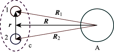
Figure 1: Schematic illustration of the system concerned in the present paper.

The system that we treat in the present study is illustrated in Fig. 1. We start with the expansion of the total wave function $\Psi$:

$$\Psi({\bf R},{\bf r})=\sum_{i\ell m}\Phi_{i,\ell m}({\bf r})\sum_{m_{0}}e^{-i(m-m_{0})\phi_{R}}\chi_{i\ell m}(R,\theta_{R}),$$ (1)

where $\ell$ is the total spin of c and $m$ is its projection on the $z$-axis taken to be parallel to the incident beam; the subscript 0 represents the initial state. $\Phi_{i,\ell m}$ is the channel wave function of c, which contains both bound and scattering states and for the latter discretization of the continuum is made. {$\Phi_{i,\ell m}$} is assumed to form an approximate complete set for a finite configuration space being significant for a reaction concerned.

We here make the following eikonal approximation:

$$\chi_{c}(R,\theta_{R})\approx\psi_{c}(b,z){\displaystyle\frac{1}{(2\pi)^{3/2}}}e^{i{\bf K}_{c}(b)\cdot{\bf R}},$$ (2)

where $c$ denotes channels {$i$, $\ell$, $m$} together and the wave number $K_{c}$ is defined by

$${\displaystyle\frac{\hbar^{2}}{2\mu}}\left(K_{c}(b)\right)^{2}=E-\epsilon_{i,\ell}-{\displaystyle\frac{\hbar^{2}}{2\mu}}{\displaystyle\frac{(m-m_{0})^{2}}{b^{2}}}$$ (3)

with $b$ the impact parameter; the direction of ${\bf K}_{c}$ is assumed to be parallel to the $z$-axis.

Inserting Eqs. (1) and (2) into the three-body Schrödinger equation neglecting the second order derivative of $\psi_{c}$, one can obtain

$${\displaystyle\frac{i\hbar^{2}}{\mu}}K_{c}^{(b)}{\displaystyle\frac{d}{dz}}\psi_{c}^{(b)}(z)=\sum_{c^{\prime}}{\cal F}^{(b)}_{cc^{\prime}}(z)\;\psi_{c^{\prime}}^{(b)}(z)e^{i\left(K_{c^{\prime}}^{(b)}-K_{c}^{(b)}\right)z},$$ (4)

where ${\cal F}^{(b)}_{cc^{\prime}}$ is the form factor, i.e., the interaction between A and each constituent of c, folded by $\Phi_{c}$ and $\Phi_{c^{\prime}}$; we put $b$ in a superscript since it is not a dynamical variable but an input parameter. Equation (4) is solved with the boundary condition $\psi_{c}^{(b)}(-\infty)=\delta_{c0}$. Since the E-CDCC equation is first-order differential one and contains no coefficient with huge angular momentum, one can easily and safely solve the equation.

Using the solution of the E-CDCC equation, the scattering amplitude with E-CDCC is given by

$$f_{c0}^{\rm E}=-{\displaystyle\frac{\mu}{2\pi\hbar^{2}}}\int\sum_{c^{\prime}}{\cal F}^{(b)}_{cc^{\prime}}(z)\,e^{-i(m-m_{0})\phi_{R}}e^{i({\bf K_{c^{\prime}}^{(b)}}-{\bf K_{c}^{\prime(b)}})\cdot{\bf R}}\,\psi_{c^{\prime}}^{(b)}(z)d{\bf R},$$ (5)

where $\mu$ is the reduced mass of the c + A system. Making use of the following forward-scattering approximation:

$$e^{i({\bf K_{c^{\prime}}^{(b)}}-{\bf K_{c}^{\prime(b)}})\cdot{\bf R}} = -K_{c}^{(b)}\sin{\theta_{f}}b\cos{\phi_{R}}+(K_{c^{\prime}}^{(b)}-K_{c}^{(b)}\cos{\theta_{f}})z$$ (6)

$$\approx -K_{c}^{(b)}\theta_{f}b\cos{\phi_{R}}+(K_{c^{\prime}}^{(b)}-K_{c}^{(b)})z,$$

one obtains

$$f_{i\ell m,i_{0}\ell_{0}m_{0}}^{\rm E}={\displaystyle\frac{1}{2\pi i}}\int\!\!\int K_{i\ell m}^{(b)}e^{-i(m-m_{0})\phi_{R}}e^{-iK_{i\ell m}^{(b)}\theta_{f}b\cos{\phi_{R}}}\left({\cal S}_{i\ell m,i_{0}\ell_{0}m_{0}}^{(b)}\!\!-\delta_{ii_{0}}\delta_{\ell\ell_{0}}\delta_{mm_{0}}\right)bdbd\phi_{R},\\$$ (7)

where the eikonal $S$-matrix elements are defined by ${\cal S}_{i\ell m,i_{0}\ell_{0}m_{0}}^{(b)}\equiv\psi_{i\ell m}^{(b)}(\infty)$.

We here discretize $f^{\rm E}$:

$$f_{i\ell m,i_{0}\ell_{0}m_{0}}^{\rm E} = {\displaystyle\frac{1}{2\pi i}}\sum_{L}K_{i\ell m}^{(b_{L}^{\rm mid})}\left[\int e^{-i(m-m_{0})\phi_{R}}e^{-iK_{i\ell m}^{(b_{L}^{\rm mid})}\theta_{f}b_{L}\cos{\phi_{R}}}d\phi_{R}\right]$$ (8)

$$\times{}\left({\cal S}_{i\ell m,i_{0}\ell_{0}m_{0}}^{(b_{L}^{\rm mid})}-\delta_{ii_{0}}\delta_{\ell\ell_{0}}\delta_{mm_{0}}\right)\int_{b_{L}^{\rm min}}^{b_{L}^{\rm max}}bdb,$$

where $b_{L}^{\rm min}$, $b_{L}^{\rm max}$ and $b_{L}^{\rm mid}$ are defined through $K_{i\ell m}^{(b_{L}^{\rm min})}b_{L}^{\rm min}=L$, $K_{i\ell m}^{(b_{L}^{\rm max})}b_{L}^{\rm max}=L+1$ and $K_{i\ell m}^{(b_{L}^{\rm mid})}b_{L}^{\rm mid}=L+1/2$, respectively. In deriving Eq. (8) we neglecting the $b$-dependence of $K_{i\ell m}^{(b)}$, $\exp[-iK_{i\ell m}^{(b)}\theta_{f}b\cos{\phi_{R}}]$ and ${\cal S}_{i\ell m,i_{0}\ell_{0}m_{0}}^{(b)}$ within small size bin of $b$ corresponding to each $L$. After manipulation one can obtain

$$f_{i\ell m,i_{0}\ell_{0}m_{0}}^{\rm E}\!\!\approx{\displaystyle\frac{2\pi}{iK_{0}}}\sum_{L}{\displaystyle\frac{K_{0}}{K_{i\ell m}^{(b_{L}^{\rm mid})}}}\sqrt{{\displaystyle\frac{2L+1}{4\pi}}}i^{(m-m_{0})}Y_{L\,m\!-m_{0}}(\hat{\bf K}^{\prime})\left({\cal S}_{i\ell m,i_{0}\ell_{0}m_{0}}^{(b_{L}^{\rm mid})}\!\!-\delta_{ii_{0}}\delta_{\ell\ell_{0}}\delta_{mm_{0}}\right),\\$$

which has a similar form to that of standard CDCC:

$$f^{\rm Q}_{i\ell m,i_{0}\ell_{0}m_{0}}\!\!\!\!\! = \!\!\!{\displaystyle\frac{2\pi}{iK_{0}}}\sum_{L}\sum_{J=|L-\ell|}^{L-\ell}\sum_{L_{0}=|J-\ell_{0}|}^{J-\ell_{0}}\sqrt{{\displaystyle\frac{2L_{0}+1}{4\pi}}}(L_{0}0\ell_{0}m_{0}|Jm_{0})(L\;m_{0}\!\!-\!m\;\ell m|Jm_{0})$$ (9)

$$\!\!\!\hskip 45.5244pt{}\times(S_{iL\ell,i_{0}L_{0}\ell_{0}}^{J}-\delta_{ii_{0}}\delta_{LL_{0}}\delta_{\ell\ell_{0}})(-)^{m-m_{0}}Y_{L\,m\!-m_{0}}(\hat{\bf K}^{\prime}).$$

The construction of the hybrid scattering amplitude $f^{\rm H}$ is rather straightforward:

$$f_{i\ell m,i_{0}\ell_{0}m_{0}}^{\rm H}\equiv\sum_{L\leq L_{\rm C}}f_{L}^{\rm Q}+\sum_{L>L_{\rm C}}f_{L}^{\rm E},$$ (10)

where $f_{L}^{\rm Q}$ ($f_{L}^{\rm E}$) is the $L$-component of $f^{\rm Q}$ ($f^{\rm E}$). $L_{\rm C}$ represents the connecting point between quantum-mechanical and classical pictures, which is chosen so that $f_{L}^{\rm E}$ coincides with $f_{L}^{\rm Q}$ for $L>L_{\rm C}$. It should be noted that Eq. (10) includes all quantum-mechanical effects being necessary and also interference between the two $L$-regions.

In the above formulation we neglect the Coulomb distortion. In order to include it, we use $\chi_{c}^{J}(R,\theta_{R})\approx\chi^{\prime J}_{c}(b,z)\phi_{c}^{\rm C}(b,z)$ instead of Eq. (2), where $\phi_{c}^{\rm C}$ is the Coulomb wave function [16]. The formulation of $f^{\rm E}$ can then be done just in the same way above.

3 Results and discussion

In order to see the validity of the hybrid calculation with CDCC and E-CDCC, we analyze ⁵⁸Ni(⁸B,⁷Be$+p$)⁵⁸Ni at 240 MeV. Parameters of the modelspace are as follows. The numbers of bin-states of ⁸B are 16, 8 and 8 for s-, p- and d-states, respectively. The maximum excitation energy of ⁸B is 10 MeV and $r_{\rm max}$ ($R_{\rm max}$) is 100 fm (500 fm). $L_{\rm max}$ is taken to be 1000 for saving computation time, which is somewhat small compared with the expected value of $L_{\rm max}$ that gives perfect convergence, i.e., $L_{\rm max}\sim 4000$.

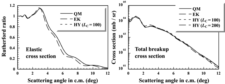
Figure 2: Angular distribution of the elastic (left panel) and total breakup (right panel) cross sections for ⁵⁸Ni(⁸B,⁷Be$+p$)⁵⁸Ni at 240 MeV. The solid, dashed and dotted lines show, respectively, the results of quantum-mechanical (QM), eikonal (EK) and hybrid (HY) calculation with $L_{\rm C}=100$. The dash-dotted line in the right panel represents HY calcualtion with $L_{\rm C}=200$.

However, the validity of the hybrid calculation can definitely be clarified in the modelspace above. As for ⁸B wave functions, the single-particle model by Kim et al. [17] was adopted. For nuclear interaction between ⁷Be ($p$) and ⁵⁸Ni we used the parameter set of Cook et al. [18] (Becchetti and Greenlees [19]); we neglected the spin-dependent part for simplicity. Additionally, we replaced Eq. (3) by $(\hbar^{2}/2\mu)K_{c}^{2}=E-\epsilon_{i,\ell}$ and neglected $c$-dependence of $K$ in the calculation of $f^{\rm E}$, which was found to have no effects on numerical results. We stress that this is not an adiabatic approximation since $K_{c}$ is explicitly treated in solving the E-CDCC equation (4).

In the left and right panels in Fig. 2 we show the elastic cross section (Rutherford ratio) and total breakup cross section as a function of scattering angle in center-of mass (c.m.) frame, respectively. The solid, dashed and dotted lines represent the results of quantum-mechanical (QM), eikonal (EK) and hybrid (HY) calculation, where the $L_{\rm C}$ are taken to be 1000, 0 and 100. In the right panel the result of HY calculation with $L_{\rm C}=200$ is also shown by the dash-dotted line. The agreement between QM and HY calculation with appropriate value of $L_{\rm C}$, namely 100 (200) for elastic (breakup) cross section, is excellent; the error is only less than 1%. One also sees fairy large difference between EK and QM calculation. Since our EK calculation contains no corrections to the straight-line approximation, this does not directly show the fail of EK approximation. However, it seems quite difficult for EK calculation to obtain “perfect” agreement with the result of QM one. On the contrary, the HY calculation turned out to be applicable to analyses of ⁸B dissociation where very high accuracy is required.

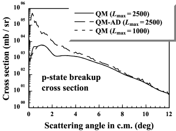
Figure 3: The p-states breakup cross sections by QM calculation with (dashed line) and without (solid line) adiabatic (AD) approximation. The maximum number of $L$ is taken to be 2500. For comparison non-adiabatic QM result with $L_{\rm max}=1000$ is shown by the dotted line.

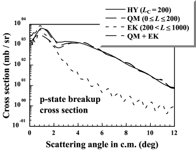
Figure 4: The p-state breakup cross sections by QM calculation with $0\leq L\leq 200$ (dashed line) and by EK calculation with $200<L\leq 1000$ (dotted line). The dash-dotted line is the incoherent sum of the dashed and dotted lines and the solid line is the HY result with $L_{\rm C}=200$, namely, the coherent sum of the two.

We show in Fig. 3 the p-state breakup cross sections by QM calculation with (dashed line) and without (solid line) adiabatic (AD) approximation. Since the convergence of AD calculation is rather slow compared with non-AD one, we take $L_{\rm max}=2500$ to make fair comparison. One sees that AD calculation much overestimates the breakup cross section, which shows the failure of AD approximation for this reaction. In Fig. 3 the non-AD QM result with $L_{\rm max}=1000$ is also shown by the dotted line. The difference between the solid and dotted lines is finite but quite small, which indicates the QM calculation with $L_{\rm max}=2500$ works well, i.e., the large difference between AD and non-AD results is indeed due to the use of AD approximation.

In Fig. 4 the p-state breakup cross sections by QM calculation with $0\leq L\leq 200$ and EK calculation with $200<L\leq 1000$ are shown by the dashed and dotted lines, respectively. The dash-dotted line is the incoherent sum of the two, which deviates from the HY result shown by the solid line. This result shows that the essence of our HY calculation is the construction of the hybrid scattering amplitude not the hybrid cross section.

4 Summary and Conclusions

In the present paper we propose a new method to treat breakup process accurately and efficiently, that is, the hybrid (HY) calculation with the Continuum-Discretized Coupled-Channels method (CDCC) and the Eikonal-CDCC method (E-CDCC). E-CDCC describes the center-of-mass (c.m.) motion between the projectile and the target nucleus by straight-line (eikonal approximation) and treats the excitation of the projectile explicitly, by constructing discretized-continuum states as in CDCC, i.e., non-adiabatic and non-perturbative calculation can be done. When Coulomb distortion appears, we make a similar approximation to the eikonal one; we use Coulomb wave functions instead of plane waves. The resultant scattering amplitude by E-CDCC has a similar form to the quantum-mechanical (QM) one obtained by CDCC, which allows one to construct HY amplitude $f^{\rm H}$ in an intuitive way; $f^{\rm H}$ is given by the sum of the partial amplitude calculated by CDCC for smaller angular momentum $L$ and that by E-CDCC for larger $L$, i.e., larger impact parameter $b$.

We analyzed ⁵⁸Ni(⁸B,⁷Be$+p$)⁵⁸Ni at 240 MeV by QM, full-eikonal (EK) and HY calculation. It was found that the elastic and total breakup cross sections obtained by QM calculation are “perfectly” reproduced by the HY calculation, namely, the error is only less than 1%. Constructing HY cross section, not HY amplitude, turned out to fail to reproduce the corresponding QM result, which shows the importance of the interference between the two $L$-regions above.

In conclusion, the hybrid calculation using CDCC and E-CDCC allows one very accurate analyses for breakup processes. The accuracy of the model is enough to be applied to ⁸B dissociation relating to the astrophysical factor $S_{17}(0)$, the aim of which is determining $S_{17}(0)$ with less than 5% errors. E-CDCC drastically reduces computaion time and eliminates many problems concerned with huge angular momentum in solving Coupled-Channels (CC) equations. Thus, the hybrid calculation opened the door to the systematic analyses of ⁸B dissociation measured at RIKEN, MSU and GSI. Extracted $S_{17}(0)$ by using the ANC method will be reported in near future.

References

- [1] J. N. Bahcall et al., Astrophys. J. 555, 990 (2001) and references therein.
- [2] J. N. Bahcall et al., JHEP 0108, 014 (2001) [arXiv:hep-ph/0106258]; JHEP 0302, 009 (2003) [arXiv:hep-ph/0212147].
- [3] A. Azhari et al., Phys. Rev. C 60, 055803 (1999); Phys. Rev. Lett. 82, 3960 (1999).
- [4] L. Trache et al., Phys. Rev. Lett. 87, 271102 (2001).
- [5] K. Ogata et al., Phys. Rev. C 67, R011602 (2003).
- [6] H. M. Xu et al., Phys. Rev. Lett. 73, 2027 (1994).
- [7] T. Motobayashi et al., Phys. Rev. Lett. 73, 2680 (1994); T. Kikuchi et al., Eur. Phys. J. A 3, 209 (1998).
- [8] N. Iwasa et al., Phys. Rev. Lett. 83, 2910 (1999).
- [9] B. Davids et al., Phys. Rev. Lett. 86, 2750 (2001); Phys. Rev. C 63, 065806 (2001).
- [10] M. Kamimura et al., Prog. Theor. Phys. Suppl. 89 (1986); N. Austern et al., Phys. Rep. 154, 125 (1987).
- [11] N. Yamashita, Master thesis, Kyushu University, 2003.
- [12] J. von Schwarzenberg et al., Phys. Rev. C 53, 2598 (1996); J. Kolata et al., Phys. Rev. C 63, 024616 (2001).
- [13] H. Esbensen and G. F. Bertsch, Phys. Rev. C 59, 3240 (1999).
- [14] R. A. D. Piyadasa et al., Phys. Rev. C 60, 044611 (1999).
- [15] N. Austern et al., Phys. Rev. Lett. 63, 2649(1989); N. Austern et al., Phys. Rev. C 53, 314 (1996).
- [16] M. Kawai, private communication (2003).
- [17] K. H. Kim et al., Phys. Rev. C 35, 363 (1987).
- [18] J. Cook, Nucl. Phys. A388, 153 (1982).
- [19] F. D. Becchetti and G. W. Greenlees, Phys. Rev. 182, 1190 (1969).