Is the nuclear force short range ?

Abstract

Possible strong Van der Waals force is searched in the nuclear interaction, whose existence is expected when the fundamental interaction between quarks is strong or superstrong Coulombic type. The relation between the type of the extra singularity at $t=0$ of the scattering amplitude and the power of the asymptotic behavior of the long range potential is derived. The square root cusp in the once subtracted S-wave amplitude, whose existence is expected when the Van der Waals force of the London type is acting, is observed when we analyze the high precision phase shift data of the low energy proton-proton scattering.

1 Van der Waals force in the composite model of hadron

Before we accepted the composite model of hadron in 1960’s, the nucleons were the elementary particles and the nuclear force was essentially the short range force arising from the exchanges of a pion and a set of pions and heavier particles. However the short range nature of the nuclear force is not necessarily correct in composite hadron, especially when the fundamental force which combines the quarks is Coulombic. It is strange that even after the acceptance of the composite model, the nuclear force is still regarded as short range with argument that, when the momentum transfer is not very large and one does not explore the inside of the composite system, we can regard the nucleon as elementary particle with good approximation. However this argument is not true, especially when the fundamental force is Coulombic. In such a case, as we shall see later, the Van der Waals interaction between hadrons must always appear. It is instructive to review the mechanism of the appearance of the Van der Waals potential between the neutral ’atoms’ and to estimate the strength $C$ of the potential in the asymptotic region

$$V(R)\sim-\frac{C}{R^{6}}\qquad in\quad R\gg a\quad,$$ (1)

where $a$ is the radius of the composite particle.

Let us consider a simple system in which two atoms are in the ground states of $L=0$, and they are fixed with separation $R$. Because of the quantum fluctuation, atoms can also stay in the excited $L=1$ state, whose duration is $\Delta t\approx\hbar/\Delta E_{1}$ by the uncertainty principle where $\Delta E_{1}$ is the excitation energy. Suppose that atom 1 is in the excited P-state and therefore has the dipole moment $\vec{d}_{1}$. The dipole must produce the field $\vec{G}$ at the location of atom 2, which decreases as $R^{-3}$ for large $R$. The field $\vec{G}$ induces a dipole $\vec{d}_{2}$ of the atom 2, which is $\alpha_{2}\vec{G}$ where $\alpha_{2}$ is the polarizability of the atom 2. The induced dipole $\vec{d}_{2}$ produces in turn a field $\vec{G^{\prime}}$ at the location of atom 1, and therefore the energy of the system changes by $-\vec{{d}_{1}}\cdot\vec{G^{\prime}}$ which decreases as $R^{-6}$ for large separation $R$. This is the mechanism of the appearance of the attractive Van der Waals potential of the London type. In particular for the case of the ordinary atoms, since the electric charge is the source of the constructive Coulomb field, the dipole $\vec{d}$ is the electric dipole and the field $\vec{G}$ is the electric field. However the mechanism to induce the Van der Waals force is more general, and any charge, which produce the fundamental Coulombic force, can do the same job. For example, the color charge in QCD or the magnetic charge in the dyon model[1] is responsible for the appearance of the Van der Waals interaction between hadrons.

In order to estimate the strength $C$ of the Van der Waals potential $V(R)\sim-C/R^{6}$, let us consider the simplest case in which atom 1 and atom 2 are respectively composed of two particles of opposite sign. As shown in fig.1, $\vec{r}_{i}$ is the relative coordinate of atom i. The interaction Hamiltonian $H^{\prime}$ of the system of atom 1 and atom 2 is

$$H^{\prime} = {}^{*}e^{2}\{\frac{1}{R}+\frac{1}{|\vec{R}+\vec{r_{2}}-\vec{r_{1}}|}-\frac{1}{|\vec{R}-\vec{r_{1}}|}-\frac{1}{|\vec{R}+\vec{r_{2}}|}\}$$ (2)

$$= \frac{{}^{*}e^{2}}{R^{3}}(x_{1}x_{2}+y_{1}y_{2}-2z_{1}z_{2})+o(\frac{1}{R^{5}})$$

, where ${}^{*}e^{2}$ is the ”fine structure constant” of the relevant charge which produces the fundamental Coulombic field. The energy shift $V(R)$ of the two-atom system is

$$V(R)=-\sum_{n\neq 0}\frac{(H^{\prime})_{0n}(H^{\prime})_{n0}}{E_{n}-E_{0}}+\cdots.$$ (3)

If we see that the numerator of each term of the summation of Eq.(3) is positive definite and the energy denominators are not less than the first excitation energy $\Delta E_{1}=E_{1}-E_{0}$, we can obtain the lower and the upper bounds of the coefficient $C$ of the Van der Waals potential by retaining only the first term and by replacing all the denominators by $\Delta E_{1}$ respectively, and which is

$$\frac{|<1|(R^{3}H^{\prime})|0>|^{2}}{\Delta E_{1}}\leq C\leq\frac{<0|(R^{3}H^{\prime})^{2}|0>}{\Delta E_{1}}\quad,$$ (4)

in the estimation of the upper bound the closure relation is used. If we substitute Eq.(1-2), the upper and the lower bounds become

$$\frac{2}{3}\frac{{}^{*}e^{4}}{(\Delta E_{1})}\hat{r}_{1}^{2}\hat{r}_{2}^{2}\leq C\leq\frac{2}{3}\frac{{}^{*}e^{4}}{(\Delta E_{1})}\bar{r_{1}}^{2}\bar{r_{2}}^{2}\quad,$$ (5)

where $\bar{r_{i}}^{2}$ is the ordinary mean square radius of the ground state of atom i. On the other hand, $\hat{r}$ is the radius, which relates to the transition amplitude, defined by

$$\hat{r}^{2}=3|\tilde{z}|^{2}\qquad with\qquad\tilde{z}=\int d^{3}r\psi^{*}_{1,1,0}(rcos\theta)\psi_{0,0,0}\quad.$$ (6)

Now we can estimate the order of magnitude of the strength $C$ of the Van der Waals potential, in which $\Delta E_{1}=2$ and the radius is $1/2\sim 1/6$ in the unit of the pion mass or the pion Compton wave length. The largest value of the radius 1/2 comes from the charge radius of the nucleon, whereas the smallest radius 1/6 is obtained from the distance of the repulsive core 1/3 of the nucleon-nucleon interaction. It is interesting that in QCD, in which ${}^{*}e^{2}\sim 0.3$, the strength $C$ becomes 0.003 even if the radius is 1/2. On the other hand in the magnetic monopole model of hadron,[1] in which ${}^{*}e^{2}\approx 137.0/4$, $C$ becomes order of 1 when the radius is 1/4$\sim$1/5, and in this case the Van der Waals interaction can compete with the nuclear force arising from the meson exchanges.

2 Can the nuclear potential be derived from the meson theory ?

In 1950’s and 60’s, the nuclear potential had been studied expensively, in which Taketani’s idea played an important roll. In his idea the nuclear force is divided into three parts according to the range. The outermost region is described by the one-pion exchange, whereas the innermost region is treated by phenomenological way and the hard core potential is used in $\mu R<x_{c}$. On the other hand in the middle region, the two-pion exchange is responsible for the nuclear potential, and which is supposed to be calculated from the interaction Lagrangian $L_{\pi,N}$ of the meson theory. In figure 2 the central potential ${}^{1}V_{C}^{+}(R)$ of the singlet even state is plotted against $R$. The curve OPE is the one-pion exchange contribution. The curve TMO is the OPE plus the two-pion exchange contribution which is computed by the standard perturbation (static), whereas HM is the same quantity with full recoil considered.[2]

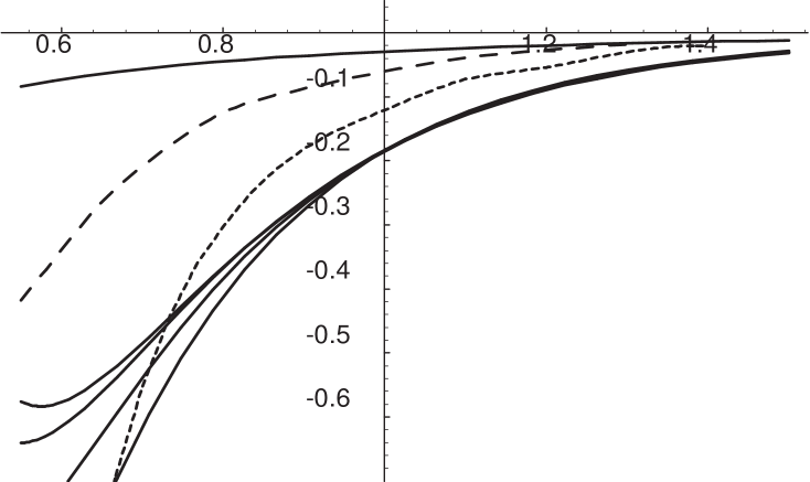
${}^{1}V^{+}_{C}(R)$

$R$

$OPE$

$HM$

$TMO$

$(d)$

$(c)$

$(b)$ $(a)$

Figure 2: Potential ${}^{1}V^{+}_{C}(R)$ is plotted against R in the unit of the neutral pion mass and its Compton wave length. The curves a(0.30), b(0.25), c(0.20) and d($0\sim 0.15$) are the one-boson exchange potentials of Eq.(2-1) fitted to the experimental data with various hard core radii, which are given in the brackets. The curve OPE is the one-pion exchange potential. The curve TMO is the OPE plus the two-pion exchange potential which is computed by the perturbation theory (static), whereas the curve HM is the same type potential with full recoils are involved. Some attractive potential seems to be missing from the theoretical curves (TMO and HM) in the region around $R\sim 1$.

On the other hand, curves a(0.30), b(0.25), c(0.20) and d($0\sim 0.15$) are the one-boson exchange potentials:

$${}^{1}V_{C}^{+}=\left\{\begin{array}[]{ll}\mu\{-(\frac{f^{2}}{4\pi})\frac{e^{-x}}{x}+A\frac{e^{-4x}}{x}+B\frac{e^{-5.5x}}{x}\}&\mbox{for $x\geq x_{c}$}\\ \infty&\mbox{for $x<x_{c}$}\end{array}\right.$$ (7)

in which $x=\mu R$ and the parameters $A$ and $B$ are determined by fitting to the phase shift data, and whose values are listed in the table below. The four curves differ by the hard core radii $x_{c}$, and whose values are written in the bracket.

$\qquad curve\qquad$	$\qquad x_{c}\qquad$	$\qquad A\qquad$	$\qquad B\qquad$
(a)	0.30	-12.1	16.2
(b)	0.25	-13.6	23.0
(c)	0.20	-14.2	26.1
(d)	0 $\sim$ 0.15	-14.8	28.2

It is evident that large attractive potential is missing from the TMO and HM potentials, and therefore these theoretical potentials can not reproduce the phase shift. In order to settle the discrepancy, it is customary to add the term of the fictitious $\sigma$-meson exchange, in which the $\sigma$-meson mass $m_{\sigma}$ and the $\sigma$-N coupling constant are free parameters. However in this paper we shall examine whether we can attribute the missing attractive force to the strong Van der Waals interaction mentioned in the previous section.

3 Extra singularity of the amplitude characteristic to the long range interaction

In order to identify the long range interaction in the nuclear force, it is important to find the behavior of the scattering amplitude $A(s,t)$ characteristic to the existence of the long range interaction. When the nuclear force arises from the meson exchanges, $A(s,t)$ has a pole at $t=1$ and the continuous spectrum $A_{t}(s,t)$ starting from $t=4$ and so on. What is important is that in such a case $A(s,t)$ is regular at $t=0$. On the other hand, when the long range force is acting, an extra singularity appears at $t=0$ and the spectral function becomes non-zero from $t=0$. Since $t=0$ is the end point of the physical region $-4\nu\leq t\leq 0$, where experimental data are available, we can in priciple determine the type and the magnitude of the singularity at $t=0$, when the precise data are available in the small neighborhood of $t=0$. The threshold behavior of the spectral function $A_{t}$ is specified by the power $\gamma$ and the coefficient $C^{\prime}$, which are defined by

$$A_{t}(s,t)=\pi C^{\prime}t^{\gamma}(1+o(t))\quad.$$ (8)

These parameters relate to the parameters $\alpha$ and $C$ of the potential $V(R)$ which are defined by $V(R)\sim-C/R^{\alpha}$ in the asymptotic region. The relations are

$$\alpha=2\gamma+3\qquad and\qquad C=\frac{2C^{\prime}}{m^{2}}\Gamma(2\gamma+2)\quad,$$ (9)

where $m$ is the reduced mass of the potential scattering.[3]

It is not difficult to derive the relations, if we remember that the potential $V(R)$ can be represented as the superposition of the Yukawa potentials:

$$V(R)=-\frac{1}{\pi m^{2}}\frac{1}{R}\int_{0}^{\infty}w(t^{\prime})e^{-R\sqrt{t^{\prime}}}dt^{\prime}\quad.$$ (10)

Since the range of the integration is from 0 to infinity, this is nothing but the Laplace transformation of $RV(R)$. What is important is that the weight function $w(t)$ is the imaginary part of the first Born amplitude $A^{(B)}(s,t)$. we can see this simply by computing the Fourier transformation of both sides of Eq.(10) and which leads to a dispersion relation of the form

$$A^{(B)}(s,t)=\frac{1}{\pi}\int_{0}^{\infty}\frac{w(t^{\prime})}{t^{\prime}-t}dt^{\prime}\quad.$$ (11)

In particular if the weight function is $w(t^{\prime})=\pi C^{\prime}t^{\prime\gamma}$, the potential of Eq.(10) becomes

$$V(R)=-\frac{2C^{\prime}}{m^{2}}\Gamma(2\gamma+2)\frac{1}{R^{2\gamma+3}}\quad.$$ (12)

Since the change of the weight function at finite $t^{\prime}$ does not alter the tail of the potential, we obtain the relations between the powers $\alpha$ and $\gamma$ and also between the coefficients $C$ and $C^{\prime}$ given in Eq.(9).

Therefore the extra singularity of the scattering amplitude $A(s,t)$ at $t=0$ is

$$A(s,t)=-\frac{\pi}{\sin\pi\gamma}C^{\prime}(-t)^{\gamma}+\cdots\quad,$$ (13)

where dots mean the background regular function and can be represented by a polynomial of $t$. When $\gamma$ is an integer $n$, we must take the limit $\gamma\rightarrow n$, and the singular term becomes $C^{\prime}t^{n}\log(-t)$. Since $t=-2\nu(1-z)$, there are two ways to observe the extra singularity at $t=0$. One is to see the angular distribution for fixed $\nu$ and to observe the singular behavior $(1-z)^{\gamma}$ at $z=1$. Second is to make the partial wave projection and to observe the singularity $\nu^{\gamma}$ at the threshold in the partial wave amplitude $a_{\ell}(\nu)$. In our normalization, $a_{\ell}(\nu)$ relate to the phase shifts in the elastic region by

$$a_{\ell}(\nu)=\frac{\sqrt{s}}{2\sqrt{\nu}}e^{i\delta_{\ell}(\nu)}\quad,$$ (14)

or in terms of the effective range function $X_{\ell}(\nu)$

$$a_{\ell}(\nu)=\frac{1}{X_{\ell}(\nu)-i\frac{2\sqrt{\nu}}{\sqrt{s}}}\quad where\quad X_{\ell}(\nu)=\frac{2\sqrt{\nu}}{\sqrt{s}}\cot\delta_{\ell}(\nu)\quad.$$ (15)

In order to make the extra singularity more visible in the search we shall use the once subtracted partial wave amplitudes which are defined by

$$a_{0}^{once}(\nu)=\frac{a_{0}(\nu)-a_{0}(0)}{\nu}\quad and\quad a_{\ell}^{once}(\nu)=\frac{a_{\ell}(\nu)}{\nu}\quad for\quad\ell\geq 1\quad.$$ (16)

In $a_{\ell}^{once}(\nu)$, the singularity is changed to $C^{\prime\prime}_{\ell}\nu^{\gamma-1}$. Therefore the extra singularity of the Van der Waals interaction of the London type must appear as the square root cusp $C^{\prime\prime}_{\ell}\nu^{1/2}$ at $\nu=0$ . Moreover since the Van der Waals force is attractive, namely $C^{\prime}>0$, the cusp must point downward.

In order to observe the extra singularity as clearly as possible, it is necessary to remove the nearby singularities and prepare the domain of analyticity of the back ground function as wide as possible. First of all we must remove the unitarity cut, whose spectral function is Im $a_{\ell}(\nu)=(\sqrt{s}/2\sqrt{\nu})\sin^{2}\delta_{\ell}(\nu)$, or in terms of the effective range function $X_{\ell}(\nu)$

$$\mbox{Im }a_{\ell}(\nu)=\frac{2\sqrt{\nu}}{\sqrt{s}}\frac{1}{X_{\ell}(\nu)^{2}+4\nu/s}\quad with\quad X_{\ell}(\nu)=\frac{2\sqrt{\nu}}{\sqrt{s}}\cot\delta_{\ell}(\nu)\quad.$$ (17)

This is done by introducing a function

$$K_{\ell}^{once}(\nu)=a_{\ell}^{once}(\nu)-\frac{1}{\pi}\int_{0}^{U}d\nu^{\prime}\frac{\mbox{Im}a_{\ell}(\nu^{\prime})}{\sqrt{\nu^{\prime}}(\nu^{\prime}-\nu)}\quad,$$ (18)

in which the domain of the integration $[0,U]$ may be chosen as the region where the reasonably accurate phase shift data are available.

The amplitude $K_{\ell}(\nu)$ is sometimes called Kantor amplitude, which is free from the singularity at $\nu=0$ when all the forces are short range. Concerning the left hand cuts, the nearest one is the cut of the one-pion exchange which starts at $\nu=(-1/4)$. Such a cut is removed in $(K_{\ell}^{once}(\nu)-a_{\ell}^{once,1\pi}(\nu))$, where

$$a_{\ell}^{once,1\pi}(\nu)=(\frac{1}{4}\frac{g^{2}}{4\pi})\frac{1}{\nu}(\frac{1}{2\nu}Q_{\ell}(1+\frac{1}{2\nu})-\delta_{\ell,0})\quad.$$ (19)

The next nearest left hand singularity appears at $\nu=-1$ which is the threshold of the two-pion exchange. Since the threshold behavior of the spectrum is $C^{\prime\prime}_{2\pi}(-1-\nu)^{3/2}\theta(-1-\nu)$, the distortion of the background function arising from the two-pion exchange in the small neighborhood of $\nu=0$ is small. Therefore we can observe the extra singularity at $\nu=0$ unless its coefficient is not very small.

4 Observation of the cusp at $\nu=0$ in the once subtracted S-wave amplitude

In order to distinguish the effect of the long range force from that of the two-pion exchange, we need accurate data. It is well known that the accuracy of the measurements of the low energy proton-proton scattering is highest in the hadron physics. Therefore we shall analyze the once subtracted S-wave amplitude of the p-p scattering $a_{0}^{once}(\nu)$, which is spin-singlet. Because of the electromagnetic interaction between protons, some modifications are necessary when we construct the once sutracted Kantor amplitude $K_{0}^{once}(\nu)$ given in Eq.(18). Contrary to the phase shift $\delta_{0}(\nu)$ of the scattering by purely short range potential, in which the incoming and the outgoing waves are the partial wave projection of the plane wave, we must use the electromagnetically distorted wave as the initial and the final states. The information of the scattering of $\ell=0$ state is summarized in the phase shift $\delta_{0}^{C}(\nu)$, $\delta_{0}^{E}(\nu)$ or $\delta_{0}^{EM}(\nu)$. The small differences of these phase shifts are due to what portion of the electromagnetic interaction is involved when we compute the distorted incoming and outgoing waves. The potentials which distort the initial and the final waves are: (C) pure Coulomb force of the point proton, (E) the Coulomb force of the proton with electric form factor plus the vacuum polarization effect or (EM) in addition to the interactions of the case E other tiny effects of the electromagnetic interactions such as the interaction between the anomalous magnetic moments of protons are involved, respectively.

The relation between the effective range function $X_{0}(\nu)$ and the phase shift of Eq.(15) must be modified. Its explicit form is given in other paper.[3][4] What is important is that the effective range function $X_{0}(\nu)$ is regular at $\nu=0$. If we notice this property, it is straightforward to construct the once subtracted Kantor amplitude $K_{0}^{once}(\nu)$ which is free from the singularity at $\nu=0$ when the interactions are short range plus electromagnetic.[3] In order to ease the search of the extra singularity, it is necessary to subtract the term of the one-pion exchange at least approximately. The S-wave phase shift data $\delta_{0}^{EM}(\nu)$ of the energy dependent analysis by Nijmegen group[5] are used in the evaluation of the once subtracted Kantor amplitude $K_{0}^{once}(\nu)$. In figure 3, $-\tilde{K}_{0}^{once}(\nu)\equiv-(K_{0}^{once}(\nu)-a_{0}^{once,1\pi}(\nu))$ is plotted against $T_{lab}$, in which the range of $T_{lab}$ is $0<T_{lab}<125\mbox{MeV.}$. Figure 4 is the same graph with enlarged scale and the narrow energy range $0<T_{lab}<20\mbox{MeV.}$. In figure 4, the error bars are attached to the data points (circles) of very low energy region, however for higher energy the error becomes smaller than the size of the data point. We can clearly see a cusp at $\nu=0$ pointing upward, which means the attractive long range force is acting.

- $\tilde{K}_{0}^{once}(\nu)$

Figure 3: $-\tilde{K}_{0}^{once}(\nu)$ is plotted against $T_{lab}$ in $T_{lab}<125\;MeV.$, in which the Nijmegen phase shift data of the energy dependent analysis are used. The curve is the fit by the spectrum of the long range force in the range $0.6\;MeV.<T_{lab}<125\;MeV.$. The graph indicates the square root cusp at $T_{lab}=0$, which points upward.

- $\tilde{K}_{0}^{once}(\nu)$

$(sa)_{3}$

$\swarrow$

Figure 4: The enlarged graph of $-\tilde{K}_{0}^{once}(\nu)$ is plotted in $T_{lab}<20\;MeV.$. The three curves are 3-parameter fits to the data in $0.6\;MeV.<T_{lab}<125\;MeV.$. The curve $(L)_{3}$ is the fit by the spectrum of the long range force, whereas the curves of $(s\;a)_{3}$ (dots) and $(s\;b)_{3}$ (dash) are the fits by the short range potentials.

In order to determine the type of the long range force, let us make the chi-square fit by the spectrum of the long range force

$$A_{t}(s,t)=\pi C^{\prime}t^{\gamma}e^{-\beta t}$$ (20)

Best fit in $0.6\mbox{MeV.}<T_{lab}<125\mbox{MeV.}$ is achieved by

$$\gamma=1.54\quad,\quad C^{\prime}=0.18\quad and\quad\beta=0.063\quad,$$ (21)

in the unit of the neutral pion mass. The curve of the best fit is shown in fig.3 and also $(L)_{3}$ curve of fig.4, which designates the long range spectrum with three parameters. On the other hand, the fits by the short range force, whose spectrum is the sum of three delta functions and their coefficients are free parameters, are shown in fig.4. For the dot curve $(sa)_{3}$, the locations of the delta functions are $t=4,9$ and $16$, whereas for the dash curve $(sb)_{3}$, the locations are $t=9,16$ and $25$ respectively. It is evident that the short range force cannot reproduce the data points well.

5 Conclusion and prospect

Since the parameters of the spectrum of the long range force are determined in Eq.(21), by using the relation Eq.(9) we can evaluate the parameters of the tail of the long range the potential $V(R)\sim-C/R^{\alpha}$, which become $\alpha=6.09$ and $C=0.18$ in the unit of the neutral pion mass. It indicates that reasonably strong Van der Waals force of the London type is acting between nucleons. Therefore contrary to the ordinary model of the nuclear potential, in which only the short range forces are involved, it is important to construct nuclear potential anew based on the strong Van der Waals interaction plus the short range potential arising from the exchanges of mesons.

If we remember the fact that the Van der Waals interaction is universal, the extra singularity at $t=0$ must occur in every amplitudes of the hadron-hadron reactions. We can expect to observe it whenever very accurate data are available, or when we can construct a back ground function with wider domain of analyticity. The low energy p-p amplitude is the former case, whereas the low energy P-wave amplitude of the pion-pion scattering belongs to the latter case. Because of the crossing symmetry we can remove the cut of the two-pion exchange as well as the unitarity cut from the $\pi$-$\pi$ amplitude, therefore we can expect to observe the cusp in $a_{1}(\nu)/\nu$ when reasonably accurate pion-pion phase shifts data are given. Details are found in separate papers.[6]

Finally from the upper bound of the strength $C$ of the Van der Waals potential given in Eq.(7), we can estimate the lower bound of the strength ${}^{*}e^{2}$ of the fundamental Coulomb interaction, it becomes

$${}^{*}e^{2}>3.06\qquad,$$ (22)

in which the values of the nucleon radius $\bar{r}=0.5$ and of the first excitation energy $\Delta E_{1}=m_{\Delta}-m_{N}=2.17$ are used as well as the strength $C=0.18$ of the Van der Waals potential. It is interesting to compare the result Eq.(22) with the strength of the QCD, which is ${}^{*}e^{2}\sim 0.3$, and also with that of the magnetic monopole model of hadron, which is ${}^{*}e^{2}=137.0/4$ by Dirac’s charge quantization condition.[1] Therefore the value of the strength $C$ of the Van der Waals potntial supports the magnetic monopole model of hadron rather than the QCD. My dream is to confirm the magnetic momopole model of hadron[1] by observing directly the monopoles of opposite sign fuse to form a meson.

References

-
[1]
J. Schwinger , Science 165 ,757 , (1969)
A. O. Barut , Phys. Rev. D3 , 1747 , (1971)
T. Sawada , Phys. Lett. B43 , 517 , (1973) -
[2]
M.Taketani, S.Machida and S.Ohnuma ,
Prog. Theor. Phys. 7, 45, (1952)
N.Hoshizaki and S.Machida , Prog. Theor. Phys. 27, 62, (1962) -
[3]
T.Sawada, Int. Journ. Mod. Phys. A11,
5365, (1996)
T.Sawada, ”Present status of the long range component in the nuclear force”, preprint NUP-A-2000-10,(hep-ph/0004080), (2000) - [4] L.Heller , Phys.Rev. 120, 627, (1960)
-
[5]
J.R.Bergervoet, P.C.van Campen, W.A. van der Sanden
and J.J.de Swart , Phys. Rev. C38 , 15 , (1988)
J.R.Bergervoet, P.C.van Campen, R.A.M.Klomp, J.L. de Kok, T.A.Rijken, V.G.J.Stokes and J.J.de Swart , Phys. Rev. C41 , 1435 , (1990)
V.G.J.Stokes, R.A.M.Klomp, M.C.M.Rentmeester and J.J.de Swart , Phys. Rev. C48 , 792 , (1993) -
[6]
T.Sawada, Phys.Lett. B225, 291, (1989)
T.Sawada, Frascati Physics Series XV, 223, (1999)
T.Sawada, Progr. in Particle and Nucl. Phys. 50 , 573 , (2003)