$\Lambda(1405)$ production in the $\pi^{-}p\to K^{0}\pi\Sigma$ reaction

Abstract

We discuss the mechanisms that lead to $\Lambda(1405)$ production in the $\pi^{-}p\to K^{0}\pi\Sigma$ reaction. The problem has gained renewed interest after different works converge to the conclusion that there are two resonances around the region of 1400 MeV, rather than one, and that they couple differently to the $\pi\Sigma$ and $\bar{K}N$ channels. We look at the dynamics of that reaction and find two mechanisms which eventually filter each one of the resonances, leading to very different shapes of the $\pi\Sigma$ invariant mass distributions. The combination of the two mechanisms leads to a shape of this distribution compatible with the experimental measurements.

I Introduction

The $\Lambda(1405)$ resonance has kept the attention of researchers for a long time. It has been suggested to be a quasi-bound $\bar{K}N$ state which appears in a coupled channel approach to the strangeness $S=-1$ meson-baryon interaction close to the $\bar{K}N$ threshold Jones:1977yk . Subsequent studies combining chiral dynamics and unitarity in coupled channels Kaiser:1995eg ; Kaiser:1997js ; Oset:1998it , have brought new light into this idea and substantiated it from the modern perspective of chiral Lagrangians. Yet, one of the theoretical surprises along these lines has been the persistent finding of two resonances close to the nominal $\Lambda(1405)$. It was already found in Ref. Fink:1990uk using the cloudy bag model that two poles, rather than one, appeared in the region around 1405 MeV with the quantum numbers of $\Lambda(1405)$, $I(J^{P})=0(1/2^{-})$. Subsequently, two similar poles have been found in Refs. Oller:2000fj ; Oset:2001cn ; Jido:2002yz ; Garcia-Recio:2002td ; Hyodo:2002pk ; Hyodo:2003qa ; Garcia-Recio:2003ks ; Nam:2003ch using chiral unitary approaches to the problem. All the different approaches agree qualitatively in the following :

• Two poles appear in the complex plane close to the 1405 MeV region.

• The pole at lower energies has a larger width than the one appearing at higher energies.

• The lower energy resonance couples strongly to $\pi\Sigma$ and weakly to $\bar{K}N$, while the opposite occurs for the resonance appearing at higher energy, although in models which do not fit the $K^{-}p$ threshold branching ratio Garcia-Recio:2002td , the couplings look more similar.

A clarification of this interesting result has been made in Ref. Jido:2003cb where the two $\Lambda(1405)$ states have been interpreted in the following way : The SU(3) decomposition of the octet representation of the $1/2^{+}$ baryons times the octet of the $0^{-}$ pseudoscalar mesons leads to a singlet and two octets (apart from the $10$, $\bar{10}$ and $27$ representations). The two octets appear degenerate in the limit of exact SU(3) symmetry, but the explicit breaking of SU(3) due to different masses of the mesons and the baryons breaks the degeneracy. When this happens, one observes two trajectories for the poles in terms of a given SU(3) breaking parameter. Two branches for $I=1$ and two for $I=0$ emerge, one of them moving to the higher energy side of the SU(3) symmetric pole and the other one moving to the lower energy side. The $I=0$ branch that moves to low energies comes very close to the singlet pole, in such a way that reactions occurring in the energy region around 1400 MeV will excite both resonances, but only one apparent bump will be seen, giving the impression that there is only one resonance. Yet, it was discussed in Ref. Jido:2003cb that, given the fact that the two resonances couple very differently to the $\bar{K}N$ and $\pi\Sigma$ states, different reactions can give more weight to one or the other resonance leading to different shapes in the $\pi\Sigma$ mass distribution. Examples were given there for possible situations and the $K^{-}p\to\Lambda(1405)\gamma$ reaction was suggested as a means to see a case in which much weight is given to the higher mass resonance, resulting in a $\pi\Sigma$ mass distribution narrower than the nominal one with the peak position shifted by about 20 MeV to higher energies.

The lesson learned in that paper is that the shape of the $\pi\Sigma$ mass distribution obtained for a certain reaction depends drastically on the dynamics of the reaction. This reopens a problem since the shape of the $\Lambda(1405)$ resonance from the $\pi\Sigma$ mass distribution was formerly assumed to be an intrinsic property of the resonance and hence independent of the reaction used to produce it. For instance, in Refs. Kaiser:1995eg ; Kaiser:1997js ; Oset:1998it ; Garcia-Recio:2002td ; Hyodo:2002pk ; Hyodo:2003qa ; Nam:2003ch , the $\pi\Sigma$ mass distribution was generated assuming

$$\frac{d\sigma}{dM_{I}}=C|t_{\pi\Sigma\to\pi\Sigma}|^{2}p_{CM}$$ (1)

with $p_{CM}$ the momentum of the pion in the $\pi\Sigma$ rest frame. In practice, this will not necessarily happen, and at least it will not in some reactions. Indeed, if one bears in mind that the $\Lambda(1405)$ resonance is built up from the multiple scattering of the coupled channels, $\bar{K}N$, $\pi\Sigma$, $\eta\Lambda$, $K\Xi$, one can produce the resonance first by producing any of these channels and then having final state interaction leading to the final $\pi\Sigma$ state. Hence, instead of Eq. (1), we should rather have

$$\frac{d\sigma}{dM_{I}}=|\sum_{i}C_{i}t_{i\to\pi\Sigma}|^{2}p_{CM}$$ (2)

with $i$ standing for any of the coupled channels, and the coefficients $C_{i}$ will depend upon the particular reaction. If there is one pole around $\Lambda(1405)$, then the shape of $|t_{i\to\pi\Sigma}|$ is almost uniquely determined independent of the channel $i$. However, when there are two poles, it depends on $i$, since the different channel $i$ couples to the poles with different strengths Jido:2003cb . Therefore, the mass distribution develops one or another shape depending on the coefficients $C_{i}$. The fact that this distribution follows Eq. (2) rather than Eq. (1), was already pointed out in Ref. Oller:2000fj . However, no attempt was done to calculate the $C_{i}$ coefficients but rather they were fitted to the data to obtain the experimental shape of the $\Lambda(1405)$ resonance.

The aim of the present work is to study the $\pi^{-}p\to K^{0}\pi\Sigma$ reaction, from which the experimental data of the $\Lambda(1405)$ resonance are usually extracted Thomas:1973uh . Another source of experimental information comes from the $K^{-}p\to\Sigma^{+}(1660)\pi^{-}$ reaction followed by $\Sigma^{+}(1660)\to\Lambda(1405)\pi^{+}$, $\Lambda(1405)\to\pi\Sigma$ Hemingway:1985pz . The purpose of the present paper is to investigate the dynamics that goes into the $\pi^{-}p\to K^{0}\pi\Sigma$ reaction, and obtain the coefficients entering Eq. (2) which determine the shape of the $\Lambda(1405)$.

In the next section, we explore the analogy of the $\pi^{-}p\to K^{0}\pi\Sigma$ reaction with the $\pi N\to\pi\pi N$ reaction making an SU(3) extrapolation of the same low energy $\pi N\to\pi\pi N$ model. In section 3, we show the results with this model, and in section 4, we look at the contribution of resonance states excited in the s-channel. Results and conclusions are shown in subsequent sections.

II Chiral amplitudes for the $\pi^{-}p\to K^{0}\pi\Sigma$ reaction

II.1 Lagrangian

In this subsection, we briefly summarize the chiral Lagrangian, that we use in the following calculations. The meson-meson Lagrangian at the lowest order needed here takes on the form Gasser:1985gg ; Meissner:1993ah

$${\cal L}_{2}=\frac{1}{12f^{2}}<(\partial_{\mu}\Phi\Phi-\Phi\partial_{\mu}\Phi)^{2}+M\Phi^{4}>\ ,$$ (3)

where $f$ is the meson decay constant, $M$ is the quark mass matrix $M=\text{diag}(\hat{m},\hat{m},m_{s})$, and the symbol $<\,>$ denotes trace of SU(3) matrices. Similarly, following Refs. Pich:1995bw ; Ecker:1995gg ; Bernard:1995dp , we write the lowest order chiral Lagrangian including the coupling of the octet of pseudoscalar mesons to the octet of $1/2^{+}$ baryons as

$$\begin{split}\mathcal{L}_{1}^{(B)}=&<\bar{B}i\gamma^{\mu}\nabla_{\mu}B>-M_{B}<\bar{B}B>\\ &+\frac{1}{2}D<\bar{B}\gamma^{\mu}\gamma_{5}\left\{u_{\mu},B\right\}>\\ &+\frac{1}{2}F<\bar{B}\gamma^{\mu}\gamma_{5}[u_{\mu},B]>\ ,\end{split}$$ (4)

where we have adopted the usual definition for the baryon field $B$, mesonic current $u_{\mu}$ and the covariant derivative $\nabla_{\mu}$ Pich:1995bw . The strengths of the $F$ and $D$ coupling constants are fixed as $F=0.51,\;D=0.75$. At lowest order in momentum, that we will keep in our study, the meson-baryon interaction Lagrangian comes from the $\Gamma_{\mu}$ term in the covariant derivative of Eq. (4) :

$$\mathcal{L}_{WT}=<\bar{B}i\gamma^{\mu}\frac{1}{4f^{2}}[(\Phi\overleftrightarrow{\partial_{\mu}}\Phi)B-B(\Phi\overleftrightarrow{\partial_{\mu}}\Phi)]>\ ,$$ (5)

which gives the Weinberg-Tomozawa interaction. Here $\Phi$ represents the octet meson field Pich:1995bw . The $D$ and $F$ terms of Eq. (4) provide the Lagrangian where odd number of mesons couple to the two baryons. We derive the meson-baryon Yukawa interaction from this term as

$$\begin{split}\mathcal{L}_{\text{Yukawa}}=&-\frac{1}{\sqrt{2}f}<D(\bar{B}\gamma^{\mu}\gamma_{5}\{\partial_{\mu}\Phi,B\})\\ &+F(\bar{B}\gamma^{\mu}\gamma_{5}[\partial_{\mu}\Phi,B])>\ ,\end{split}$$ (6)

and the $MMMBB$ (three meson-two baryon) contact interaction as

$$\begin{split}\mathcal{L}_{\text{Contact}}=&\frac{1}{12\sqrt{2}f^{3}}<D(\bar{B}\gamma^{\mu}\gamma_{5}\{(\partial_{\mu}\Phi(\Phi^{2})\\ &-2\Phi\partial_{\mu}\Phi(\Phi)+\Phi^{2}\partial_{\mu}\Phi),B\})\\ &+F(\bar{B}\gamma^{\mu}\gamma_{5}[(\partial_{\mu}\Phi(\Phi^{2})\\ &-2\Phi\partial_{\mu}\Phi(\Phi)+\Phi^{2}\partial_{\mu}\Phi),B])>\ .\end{split}$$ (7)

II.2 Construction of the chiral amplitude

We construct a model for the $\pi^{-}p\to K^{0}\pi\Sigma$ reaction at energies close to threshold for the $\pi^{-}p\to K^{0}\Lambda(1405)$ production. This means a total center of mass energy $\sqrt{s}\sim 2$ GeV, or equivalently a three momentum of the initial pion $p_{\pi}\sim 1.7\text{ GeV}/c$ in the Laboratory frame.

Formally, we can separate the process into two parts. The first one which involves tree level $\pi^{-}p\to K^{0}MB$ amplitudes, and a second part which involves the final state interaction $MB\to\pi\Sigma$, which eventually generates a resonance if kinematical and dynamical conditions allow for it. This is shown in Fig. 1.

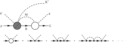
Figure 1: Diagrams entering the production of the $\Lambda(1405)$ in the $\pi^{-}p\to K^{0}\Lambda(1405)\to K^{0}\pi\Sigma$. In the figure, $M$ and $B$ stand for the meson and baryon of the 10 possible coupled channels. The $\Lambda(1405)$ resonance is dynamically generated by the final state interaction of $M$ and $B$.

We produce dynamically the $\Lambda(1405)$ via the final state interaction, as it was done for the photoproduction of the $\Lambda(1405)$ in the $\gamma p\to K^{+}\Lambda(1405)$ Nacher:1998mi . This is accomplished by summing the series of diagrams depicted in Fig. 1 via the Bethe-Salpeter equation in coupled channels Oset:1998it

$$t=V+VGT\ ,$$ (8)

with the kernel $V$ obtained from the lowest order chiral Lagrangians of Eq. (5). The coupled channels appearing in this problem are $K^{-}p$, $\bar{K}^{0}n$, $\pi^{0}\Lambda$, $\pi^{0}\Sigma^{0}$, $\eta\Lambda$, $\eta\Sigma^{0}$, $\pi^{+}\Sigma^{-}$, $\pi^{-}\Sigma^{+}$, $K^{+}\Xi^{-}$, $K^{0}\Xi^{0}$. In the following, the meson-baryon channels are numbered according to this ordering.

Concerning the initial process, the hatched blob in Fig. 1 is given by the sum of meson pole terms and contact terms as shown in Fig. 2. From the Lagrangian of Eq. (3) we obtain the meson-meson amplitude of order $f^{-2}$ and from the Lagrangian of Eq. (4) ($D$ and $F$ terms), at order $f^{-1}$, the meson-baryon-baryon coupling as shown in Eq. (6). In this way we get an amplitude at lowest order of $\mathcal{O}(f^{-3})$, which requires for consistency to calculate the order $\mathcal{O}(f^{-3})$ from the $D$ and $F$ terms of Eq. (4) by expanding $u_{\mu}$ in the number of meson fields up to three as shown in Eq. (7). This generates the contact term of Fig. 2 (b).

Figure 2: Basic terms entering the threshold production of pions in $\pi N\to\pi\pi N$. (a) : meson pole term, (b) contact term.

II.3 On-shell factorization

One interesting observation in Ref. Oset:1998it is that the $V$ amplitudes can be factorized on-shell (as a function of $s$) inside the meson-baryon loops appearing in Fig. 1. In the present case there is also an on-shell factorization for the initial process $\pi^{-}p\to K^{0}MB$ as we discuss briefly. This process is then followed by the final state interaction, shown by the open blob.

For that purpose, let us consider the one loop diagram of Fig. 3 (a).

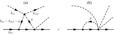
Figure 3: One loop functions for $MB\to MMB$.

In the following, we first show the factorization of the meson-meson amplitude with the momentum $q$ on-shell, then show the cancellation of the off-shell part of the meson-meson amplitude associated to the momentum $k_{in}-k_{out}-q$. With these arguments, the on-shell factorization of the meson-baryon loops Oset:1998it can be applied to the present initial process, and we can calculate the whole amplitude by evaluating the initial process at the tree level, separated from the subsequent meson-baryon loops.

Let us start with showing that the meson-meson amplitude factorizes in Fig. 3 (a) with the momentum $q$ on-shell. The $s$-wave meson-meson amplitudes from the chiral Lagrangians at lowest order have the form Oller:1997ti

$$t_{MM}=as+\sum_{i}b_{i}m_{i}^{2}+\sum_{i}\beta_{i}(q_{i}^{2}-m_{i}^{2})\ ,$$ (9)

where the term with $\beta$ gives the off-shell extrapolation of the amplitude. If we take just this off-shell part for the meson of momentum $q$ in Fig. 3 (a), the loop function reads as

$$\begin{split}&\int\frac{d^{4}q}{(2\pi)^{4}}(q^{2}-m^{2})\frac{1}{q^{2}-m^{2}}D_{\pi}(k_{in}-k_{out}-q)\\ &\quad\times G_{N}(p_{in}+k_{in}-k_{out}-q)\bm{\sigma}\cdot(\bm{k}_{in}-\bm{k}_{out}-\bm{q})\end{split}$$ (10)

using the non relativistic form $(\bm{\sigma}\cdot\bm{p})$ for the $MBB$ vertex, which will be improved later on to account for relativistic corrections. One should note that in Eq. (10), the off-shell part of the meson-meson amplitude cancels the meson propagator and leads to a contracted diagram of the type of Fig. 3 (b). On the other hand, it is interesting to note that genuine diagrams of the type of Fig. 3 (b) appear from the consideration of the $BBMMMM$ terms that come from an expansion in the meson fields of the chiral Lagrangian. These terms should be added for consistency. However, by changing $\bm{q}$ to the $\bm{p}$ variable of Fig. 3 (b) in the loop functions and realizing that the dominant term in the $\gamma^{\mu}\partial_{\mu}$ structure of the $BBMMMM$ vertex comes from the $\gamma^{0}\partial_{0}$ component (and hence no three momentum dependence), the loop functions of Fig. 3 vanish at this order (corrections coming at order $\mathcal{O}(1/2M)$).

There is also a cancellation of the off-shell part of the meson-meson amplitude for the meson with momentum $k_{in}-k_{out}-q$ in Fig. 3 (a). It appears already at tree level, but it comes from an exact cancellation between the off-shell part of the meson pole term and the contact term. This fact justifies the attempt to find out the on-shell $\pi\pi$ scattering amplitude from analysis of the $\pi N\to\pi\pi N$ data omitting the contact term Lange:2000xu , except for the contribution of other terms in the process Oset:1985wt . This off-shell cancellation found here is important conceptually. In practice, we just calculate the meson pole term with the $p_{ex}$ variable off-shell and add the contact term in each case, and the cancellation takes place automatically.

Next we look into a possible contribution from the $p$-wave part of the meson-meson amplitude. As anticipated, we are looking at the $\pi^{-}p\to K^{0}\pi\Sigma$ reaction close to threshold of the $\bar{K}N$ production in $\pi^{-}p\to K^{0}\bar{K}N$. This means that three momenta of the three final particles in the $\pi^{-}p\to K^{0}MB$ are negligible with respect to their energies. Therefore, the on-shell factorization will just pick up the $s$-wave part of the $MM$ amplitude. One might argue that the $p$-wave part of the meson-meson amplitude will not be small when taken inside loops. By looking again to the diagram of Fig. 3 (a), the $p$-wave part of the amplitude would lead to a contribution in the loops of the type

$$\begin{split}&\int d^{4}q\bm{k}_{in}\cdot\bm{q}D_{\pi}(k_{in}-k_{out}-q)D(q)\\ &\quad\times G(p_{in}-k_{in}-k_{out}-q)\bm{\sigma}\cdot(\bm{k}_{in}-\bm{k}_{out}-\bm{q})\end{split}\ .$$ (11)

Since we know that $k_{in}\sim 1500\text{ MeV}/c$ and the $q$ integral has a cut off of $600\text{ MeV}/c$ Oset:1998it , $(q/k_{in})^{2}$ is a small quantity which would allow one to take a constant propagator for the meson of momentum $k_{in}-k_{out}-q$. Since $\bm{k}_{out}\sim 0$, the term with $(\bm{k}_{in}\cdot\bm{q})\,(\bm{\sigma}\cdot\bm{k}_{in})$ vanishes in the integral, but there remains an integral

$$\int d^{4}q\,(\bm{k}_{in}\cdot\bm{q})\,(\bm{\sigma}\cdot\bm{q})D(q)G_{N}(p_{in}-k_{in}-k_{out}-q)\ ,$$ (12)

which should be reasonably smaller than the corresponding term from the meson meson s-wave which is proportional to $\bm{\sigma}\cdot\bm{k}_{in}$. Yet, there is more to it. With $\bm{k}_{in}+\bm{p}_{in}=\bm{0}$, and $\bm{k}_{out}\sim 0$, the argument of $G$ depends on $\bm{q}^{2}$ and we are left with an integral of the type

$$\begin{split}&\int d^{4}qq_{i}q_{j}D(q)G_{N}(p_{in}-k_{in}-k_{out}-q)\\ \sim&\frac{1}{3}\delta_{ij}\int d^{4}q\bm{q}^{2}D(q)G_{N}(p_{in}-k_{in}-k_{out}-q)\end{split}\ .$$ (13)

After performing the $q^{0}$ integration, we are left with an integral

$$\bm{\sigma}\cdot\bm{k}_{in}\int d^{3}q\frac{1}{2\omega(q)}\frac{\bm{q}^{2}}{M_{I}-\omega(q)-E(q)+i\epsilon}\ ,$$ (14)

with $M_{I}$ the invariant mass of the $MB$ system and $\omega$, $E$ the meson, baryon energies. The zero in the denominator of Eq. (14) gets the on-shell condition for a momentum $q_{on}$ and we can write

$$\begin{split}\bm{q}^{2}&=\omega(q)^{2}-\omega(q_{on})^{2}+\bm{q}_{on}^{2}\\ M_{I}-\omega(q)-E(q)&=\omega(q_{on})-\omega(q)+E(q_{on})-E(q)\end{split}$$ (15)

By neglecting $E(q^{on})-E(q)$ which holds in the heavy baryon limit (we are all around neglecting $1/M$ terms), the off-shell part of Eq. (14) leads to

$$\int d^{3}q\frac{1}{2\omega(q)}\frac{\omega(q)^{2}-\omega(q_{on})^{2}}{\omega(q_{on})-\omega(q)}\sim\int d^{3}q\frac{\omega(q)^{2}-\omega(q_{on})^{2}}{\omega(q_{on})^{2}-\omega(q)^{2}}\ ,$$ (16)

which is constant in energy. This energy independent term, multiplying the $\bm{\sigma}\cdot\bm{k}_{in}$ factor, can be reabsorbed into, for instance, the contact term with the use of renormalized coupling constants, say the physical values of $f_{\pi}$.

II.4 Factorized amplitude

With the arguments given above, our approach will require the evaluation of the meson pole and contact terms for the ten coupled channels $\pi^{-}p\to K^{0}M_{i}B_{i}$, using the $s$-wave $MM\to MM$ amplitude where the $\pi^{-}K^{0}M_{i}$ are factorized on-shell. Since we also saw that the intermediate propagator with momenta $k_{in}-k_{out}-q$ could also be factorized, this means we factorize the whole $\pi^{-}p\to K^{0}M_{i}B_{i}$ amplitude on-shell outside the loop integral. The remaining loop function contains only the meson of momentum $q$ and baryon propagators and this is the $G_{MB}(M_{I})$ function found out in the study of the meson-baryon interaction in Ref. Oset:1998it . Hence the whole amplitude for the process $\pi^{-}p\to K^{0}\pi\Sigma$ corresponding to the upper diagrams of Fig. 1 is given by

$$\begin{split}-it_{\text{chiral}}=&\bm{\sigma}\cdot\bm{k}_{in}\Bigl{[}(a_{\pi\Sigma}+b_{\pi\Sigma})\\ &+\sum_{i}(a_{i}+b_{i})G_{i}(M_{I})t_{i\to\pi\Sigma}(M_{I})\Bigr{]}\end{split}\ ,$$ (17)

where $i$ runs for the ten coupled channels, $t_{i\to\pi\Sigma}$ is the transition T-matrix from the channel $i$ to $\pi\Sigma$ studied in Ref. Oset:1998it and $a_{i}$, $b_{i}$ are the on-shell contributions to the $\pi^{-}p\to K^{0}M_{i}B_{i}$ tree level amplitude from the meson pole and contact terms, respectively. In the appendix, we give the $a_{i}$ and $b_{i}$ terms for all the ten channels, where, as mentioned before, we have already assumed the three momenta of the final particle negligible in all channels.

For completeness, we also include a recoil factor from the $\gamma^{\mu}\gamma_{5}\partial_{\mu}$ BBM vertex

$$F_{i}=\left(1-\frac{p_{ex}^{0(i)}}{2M_{p}}\right)\ .$$ (18)

In addition, we also consider the strong form factor of the $MMB$ vertex for which we take a standard monopole form factor for all vertices

$$F_{f}(\bm{p})=\frac{\Lambda^{2}-m_{\pi}^{2}}{\Lambda^{2}+\bm{p}^{2}}$$ (19)

with $\Lambda\sim 800$ MeV. We take the form factor static to avoid the fictitious poles of the covariant $(\Lambda^{2}-m^{2})/(\Lambda^{2}-p^{2})$ form. But we have checked that using this latter form only changes the results at the level of less than 5 %. Given the cancellation of the off-shell part of the meson pole term with the contact term, which makes the sum of the two terms independent of a possible unitary transformation in the fields, the form factor is applied both in the meson pole and the contact term. This is analogous to what is done with the pion pole and Kroll-Ruderman term in $\gamma N\to\pi N$ to preserve gauge invariance Carrasco:1992vq .

III Results with the chiral amplitudes

We perform the calculations for an initial pion momentum of 1.69 GeV, at which the experiment is done. The $\pi\Sigma$ invariant mass distribution is given by

$$\begin{split}\frac{d\sigma}{dM_{I}}=&\frac{1}{(2\pi)^{3}}\frac{1}{4s}\frac{M\tilde{M}}{\lambda^{1/2}(s,M^{2},m_{\pi}^{2})}\frac{1}{M_{I}}\\ &\times\lambda^{1/2}(s,M_{I}^{2},m_{K}^{2})\lambda^{1/2}(M_{I}^{2},\tilde{M}^{2},m^{2})\bar{\Sigma}\Sigma|t|^{2}\end{split}\ ,$$ (20)

where $M$ and $\tilde{M}$ are the masses of the nucleon and the baryon of the final state, in this case a $\Sigma$, and $m$ the mass of the final meson, in this case a $\pi$.

The distributions are calculated for $\pi^{+}\Sigma^{-}$, $\pi^{-}\Sigma^{+}$ and $\pi^{0}\Sigma^{0}$ in the final states. According to the findings of Ref. Nacher:1998mi in the $\Lambda(1405)$ photoproduction, the $I=1$ contribution approximately cancels in the sum of the $\pi^{+}\Sigma^{-}$, $\pi^{-}\Sigma^{+}$ contributions and the $\pi^{0}\Sigma^{0}$ does not have $I=1$ contribution, such that $\sigma(\pi^{+}\Sigma^{-})+\sigma(\pi^{-}\Sigma^{+})\sim 2\sigma(\pi^{0}\Sigma^{0})$ and both distributions give the $I=0$ contribution to the process, hence the $\Lambda(1405)$ contribution.

In Fig. 4, we can see the results obtained with these mechanisms compared to the experimental distribution from Ref. Thomas:1973uh .

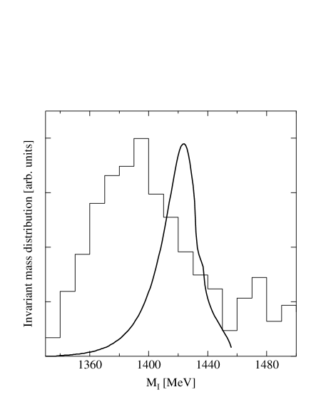
Figure 4: Contribution of the meson pole and contact terms (diagrams of Fig. 1) to the $\pi\Sigma$ invariant mass obtained averaging $\pi^{+}\Sigma^{-}$ and $\pi^{-}\Sigma^{+}$. The histogram show the experimental data taken from Ref. Thomas:1973uh .

We can see that the theoretical distribution peaks around 1420 MeV while the experimental one has the peak around 1400 MeV. The theoretical distribution is also much narrower than experiment. The disagreement between theory and experiment is apparent.

We can easily trace back the origin of the shape of the theoretical distribution. Indeed, the tree amplitude $\pi^{-}p\to K^{0}M_{i}B_{i}$ for the case of $M_{i}B_{i}=\bar{K}N$ involve the combinations $3F-D$ and $D+F$, which are large compared to the $D-F$ combination that we find for $M_{i}B_{i}\equiv\pi\Sigma$ (we take $F=0.51$ and $D=0.75$). Therefore, that the sum of the terms in Eq. (17) is dominated by the $\bar{K}N$ terms, giving a larger weight to the $t_{\bar{K}N\to\pi\Sigma}$ amplitude than to the $t_{\pi\Sigma\to\pi\Sigma}$ one. As we mentioned, the $\bar{K}N$ states couple strongly to the $\Lambda(1405)$ resonance of higher energy and weakly to the $\Lambda(1405)$ of lower energy. As a consequence, what we see is a distribution which mostly peaks around the resonance found in Ref. Jido:2003cb at the pole position $z_{R}\sim(1426+i16)$ MeV, with a width of around 30 MeV. The slightly smaller energy of the peak in Fig. 4 and larger width reflects the small contribution of the resonance of lower energies, also present in the $t_{\bar{K}N\to\pi\Sigma}$, as well as from the $t_{\pi\Sigma\to\pi\Sigma}$ amplitudes in the sum of Eq. (17), which are dominated by the lower energy $\Lambda(1405)$ resonance. This latter one appears at $z_{R}=1390+i66$ MeV.

IV The s-channel resonance contribution

Since we have $\sqrt{s}\sim 2$ GeV, one could think of the possibility of having resonance excitation in the $\pi N$ collision leading to the decay of the resonance in $MMB$. We would like to have some resonance that can couple to the $MMB$ strongly in $s$-wave. All $S=0$ baryon resonances in the region of $1700\leq\sqrt{s}\leq 2100$ MeV correspond to higher partial waves in the $\pi N$ collision, except for the $N^{*}(1710)$ and the $N^{*}(2100)$, which are $P_{11}$ resonances with the same quantum numbers of the nucleon Hagiwara:2002fs . Out of these two, the $N^{*}(1710)$ resonance has a very large branching ratio to $\pi\pi N$ (40-90%), while the one of the $N^{*}(2100)$ is unknown, probably small, since the large branching ratio seems to be for $N\eta$ (with large errors). We thus rely upon the $N^{*}(1710)$ resonance to provide some contribution to the $\pi^{-}p\to K^{0}\pi\Sigma$ process. Although one can derive different couplings of this resonance to the $MMB$ in an SU(3) scheme (see Ref. Oset:2000ev for analogy in other $P_{11}$ resonances), the absence of the kinematically allowed $\eta\pi N$ channel in the decay mode of the $N^{*}(1710)$ strongly suggest a Weinberg-Tomozawa like coupling where this mode is strictly forbidden at the tree level (see $C_{ij}$ coefficients in Refs. Inoue:2001ip ; Hyodo:2003dt ). This also has the implicit assumption that the $N^{*}(1710)$ resonance belongs to an SU(3) octet representation, which is the option adopted in the particle data table Hagiwara:2002fs . We then assume a coupling of the type of

$$\mathcal{L}_{N^{*}\to MMB}=\frac{\tilde{B}}{f^{2}}<\bar{B}i\gamma^{\mu}[(\Phi\overleftrightarrow{\partial_{\mu}}\Phi)B^{*}-B^{*}(\Phi\overleftrightarrow{\partial_{\mu}}\Phi)]>\ ,$$ (21)

where now $n^{*}(1710)$ and $p^{*}(1710)$ would substitute in the $B^{*}$ matrix as the $n$ and $p$. This Lagrangian is the same that appears in the $s$-wave scattering of meson-baryon Oset:1998it as we have seen in Eq. (5). The Lagrangian of Eq. (21) leads to the amplitude

$$t_{N^{*}\to MMB}=-\frac{\tilde{B}}{f^{2}}C_{i}(\omega_{1}-\omega_{2})\ ,$$ (22)

where $\omega_{1}$, $\omega_{2}$ are the energies of the two mesons and $C_{i}$ are the $C_{ij}$ SU(3) coefficients found in Oset:1998it ; Inoue:2001ip ; Hyodo:2003dt and reproduced below in Table 1 for the $N^{*}$ with zero charge going to pions and

Table 1: The $C_{i}$ coefficients entering Eq. (22).

	$\pi^{-}\pi^{0}p$	$\pi^{+}\pi^{-}n$	$\pi^{0}\pi^{0}n$
$C_{i}$	$-\sqrt{2}$	$1$	$0$

in Table 2 for $N^{*}$ going to $K^{0}MB$.

Table 2: The $C_{i}$ coefficients entering Eq. (22) with a $K^{0}$ in the final state.

	$K^{-}K^{0}p$	$\bar{K}^{0}K^{0}n$	$\pi^{0}K^{0}\Lambda$	$\pi^{0}K^{0}\Sigma^{0}$	$\eta K^{0}\Lambda$
$C_{i}$	$1$	$2$	$-\frac{\sqrt{3}}{2}$	$\frac{1}{2}$	$\frac{3}{2}$
	$\eta K^{0}\Sigma^{0}$	$\pi^{+}K^{0}\Sigma^{-}$	$\pi^{-}K^{0}\Sigma^{+}$	$K^{+}K^{0}\Xi^{-}$	$K^{0}K^{0}\Xi^{0}$
$C_{i}$	$-\frac{\sqrt{3}}{2}$	$1$	$0$	$0$	$0$

The $\tilde{B}$ coefficient is easily derived from the partial decay width $N^{*}\to\pi^{+}\pi^{-}n,\pi^{-}\pi^{0}p$, where we have

$$\Gamma_{\pi\pi N}=\frac{MM_{R}}{16\pi^{3}\sqrt{s}}\int_{\omega_{min}}^{\omega_{max}}d\omega\int_{\omega_{min}}^{\omega_{max}}d\omega^{\prime}\Theta(1-a^{2})\bar{\Sigma}\Sigma|t|^{2}\ ,$$ (23)

where $\Theta(x)$ is a step function and

$$a=\frac{1}{2kk^{\prime}}\Bigl{\{}(M_{R}-\omega-\omega^{\prime})^{2}-M^{2}-k^{2}-k^{\prime 2}\Bigr{\}}\ ,$$ (24)

with $k$, $k^{\prime}$ the moduli of the two pion momenta and

$$\bar{\Sigma}\Sigma|t|^{2}=3\frac{\tilde{B}^{2}}{f^{4}}(\omega-\omega^{\prime})^{2}\ .$$ (25)

Similarly, the $\pi^{-}p\to N^{*}$ coupling is given by (including the isospin factor)

$$-it=\frac{A}{f}\bm{\sigma}\cdot\bm{k}_{in}\ ,$$ (26)

by means of which the partial decay width is given by

$$\Gamma_{\pi N}=\frac{1}{2\pi}\frac{M}{\sqrt{s}}\frac{A^{2}}{f^{2}}k_{in}^{3}\ .$$ (27)

Assuming the middle values of the $N^{*}$ width ($\Gamma\sim 100$ MeV) and partial decay widths for $\pi\pi N$ and $\pi N$ channels ($\Gamma_{\pi\pi N}=65$ MeV and $\Gamma_{\pi N}=15$ MeV), we find

$$|A|=0.086\ ,\quad\tilde{|B|}=0.77\ .$$ (28)

For later convenience, we refer to this parameter set including $M_{R}=1710$ MeV as Set I.

The $\pi^{-}p\to K^{0}\pi\Sigma$ production via $N(1710)$ and $\Lambda(1405)$ production is now given diagrammatically in Fig. 5.

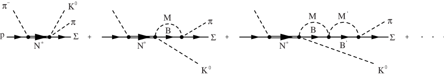
Figure 5: Resonant mechanisms for $\Lambda(1405)$ production in the $\pi^{-}p\to K^{0}\pi\Sigma$ reaction.

The amplitude for $\pi\Sigma$ production is now given by

$$\begin{split}-it_{R}=&\frac{A}{f}\bm{\sigma}\cdot\bm{k}_{in}\frac{i}{\sqrt{s}-M_{R}+i\frac{\Gamma}{2}}(-i)\frac{(-)\tilde{B}}{f^{2}}\\ &\times\Bigl{[}C_{\pi\Sigma}(\omega_{\pi}-\omega_{K^{0}})\\ &+\sum_{i}C_{i}(\omega_{i}-\omega_{K^{0}})G_{i}(M_{I})t_{i\to\pi\Sigma}\Bigr{]}\end{split}\ ,$$ (29)

with $\pi\Sigma=\pi^{0}\Sigma^{0},\pi^{-}\Sigma^{+},\pi^{+}\Sigma^{-}$, and $\omega_{i}$, $\omega_{K^{0}}$ given by their on-shell values, following the same arguments used in Ref. Oset:1998it to factorize the $MB\to MB$ amplitude on-shell in the loops,

$$\omega_{K^{0}}=\frac{s+m_{K}^{2}-M_{I}^{2}}{2\sqrt{s}}\ ,\quad\omega_{i}=\frac{M_{I}^{2}+m_{i}^{2}-M_{i}^{2}}{2M_{I}}\ ,$$ (30)

with $m_{i},M_{i}$ the meson and baryon masses of the particle in the $N^{*}\to K^{0}MB$ reaction, and $M_{I}$ the $\pi\Sigma$ invariant mass. Furthermore, in Eq. (29) $\Gamma$ is the total width whose energy dependence is taken into account by using Eqs. (23) and (27) for the $\pi\pi N$ and $\pi N$ channels, respectively, and by considering a $k^{3}$ dependence for the $\eta N$ channel.

V Results with the resonant mechanism : Final results

In Fig. 6, we show the results that we obtain for the resonant mechanism (dashed line) with Set I, together with the results obtained before from the chiral mechanisms (dotted line). The calculation was performed at the energy $\sqrt{s}=2020$ MeV, or equivalently $p_{\pi}=1690$ MeV in the laboratory frame. This is the energy at which the experiment we compare with was done Thomas:1973uh . Although the figure is shown in arbitrary units, we have adjusted the relative scale between the experimental and theoretical curves assuming that the integrated experimental mass distribution should coincide with the total cross sections in the $\pi\Sigma$ channels given in Ref. Thomas:1973uh . Theoretical and experimental total cross sections for various channels are shown in Table 3.

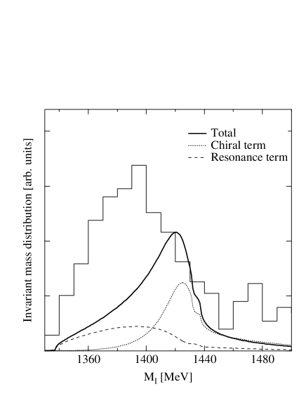
Figure 6: Invariant mass distribution of $\pi\Sigma$ obtained by averaging $\pi^{+}\Sigma^{-}$ and $\pi^{-}\Sigma^{+}$ with parameter Set I. The histogram shows the experimental data taken from Ref. Thomas:1973uh

We can see that the strength of the resonant mechanism is smaller than that of the chiral terms, however, the $\pi\Sigma$ distribution created by the resonant mechanism is much broader and peaks around 1390 MeV. It is instructive to see the reason for the shape of the resonant mechanism. Indeed, we have seen that the $N^{*}\to NM_{1}M_{2}$ vertex goes like $\tilde{B}(\omega_{1}-\omega_{2})$. Now for the case of the $K^{0}\bar{K}N$ channel, the amplitude goes like $\omega_{K^{0}}-\omega_{\bar{K}}$, but we are at low energies, close to the $K^{0}\bar{K}N$ threshold production, where the difference of the two kaon energies is close to zero. On the other hand, in the $N^{*}\to K^{0}\pi\Sigma$, the difference between the $K^{0}$and $\pi$ energies is finite and of the order of 300 MeV in the region that we study. Hence, the $K^{0}\pi\Sigma$ channel is strongly favored and according to Eq. (29), the final $\pi\Sigma$ production channel is practically given by $t_{\pi\Sigma\to\pi\Sigma}$. The factors $(\omega_{i}-\omega_{K^{0}})$ and $G_{i}(M_{I})$ give extra weight to this amplitude to finally produce a distribution that essentially reflects the lower energy $\Lambda(1405)$ resonance to which the $\pi\Sigma$ channel couples strongly.

The coherent sum of the two mechanisms, taking $A\cdot\tilde{B}>0$, leads to a mass distribution, given by the solid line, which still remains to be dominated by the chiral terms and the agreement with the data is not very good.

It is possible to improve the theoretical mass distribution if we play a bit with uncertainties in the resonance mass, the total $N^{*}$ width and the branching ratios. By assuming $M_{R}\sim 1740$ MeV, $\Gamma=200$ MeV and $\Gamma_{\pi N}=40$ MeV and $\Gamma_{\pi\pi N}=100$ MeV (We refer to this parameter set as Set II) well within the experimental boundaries, we obtain the results of Fig. 7 where the agreement with the data becomes acceptable. The increase in the resonant part is mostly due to the increase in the $\pi NN^{*}(1710)$ coupling constant when using the larger partial width $\Gamma_{\pi N}=40$. In Table 3, we have summarized cross sections of various channels comparing experimental data and theoretical results with the two sets of parameters. Except for the $K^{0}\pi^{0}\Lambda$ channel in which $\Sigma(1380)$ resonance, not accounted for in our study, plays a major role, the agreement between theory and experiment is acceptable for Set II. We can also see that the use of Set II not only improves the mass distribution but also the global agreement with the individual cross sections. Note the importance of the interference in the chiral and resonant terms in order to obtain a better agreement between theory and experiment.

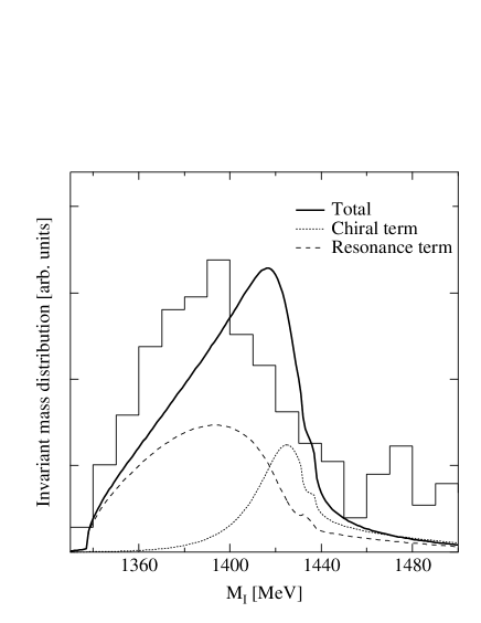
Figure 7: Same as in Fig. 6 but with Set II.

Table 3: Total cross sections for several final states with parameter sets I and II in units of [$\mu$b]. Experimental data are taken from Ref. Thomas:1973uh .

final state	$K^{0}K^{-}p$	$K^{0}\bar{K}^{0}n$	$K^{0}\pi^{0}\Lambda$	$K^{0}\pi^{+}\Sigma^{-}$	$K^{0}\pi^{-}\Sigma^{+}$
chiral	2.36	2.84	003.14	3.04	6.78
resonance(I)	0.29	0.28	004.47	6.68	2.24
resonance(II)	0.70	0.67	10.85	16.18	5.43
total(I)	2.82	4.61	001.93	12.00	14.31
total(II)	3.75	5.98	006.02	21.32	20.01
Exp.	2.9	8.3	104.0	25.1	20.2

VI Conclusions

We have developed a model for the $\pi^{-}p\to K^{0}\pi\Sigma$ reaction in the region of excitation of the $\Lambda(1405)$ resonance. We discussed the fact that present theoretical models using chiral dynamics and coupled channel unitarization are all converging to the existence of two poles close to the nominal $\Lambda(1405)$ resonance. They would reflect the singlet and one $I=0$ octet (although with some mixture), which are dynamically generated in these approaches. The two resonances appear at different energies and couple very differently to the $\pi\Sigma$ and $\bar{K}N$ channels.

When we try to construct a model for the $\pi^{-}p\to K^{0}\pi\Sigma$ in analogy to the low energy chiral model for $\pi N\to\pi\pi N$, we observe that the chiral model stresses the role of $\bar{K}N$ intermediate state making the total amplitude for $\pi^{-}p\to K^{0}\pi\Sigma$ mostly sensitive to the $t_{\bar{K}N\to\pi\Sigma}$ amplitude, which is dominated by a narrow resonance peaking at 1426 MeV. The mechanism alone leads to a $\pi\Sigma$ mass distribution in strong disagreement with the experimental data.

On the other hand, it was found that there are complementary mechanisms exciting $N^{*}$ resonances from the $\pi^{-}p$ entrance channel. Inspection of the partial waves involved in the resonance excitations and the decay modes singled out a resonance which gives contribution to the process, the $N^{*}(1710)$, with the same quantum numbers of the nucleon. The strong $N\pi\pi$ decay channel together with the absence of the $N\pi\eta$ channel, suggested a coupling of the $N^{*}(1710)$ resonance to $BMM$ of the SU(3) Weinberg-Tomozawa type, which we exploited to see the consequences in the $\pi^{-}p\to K^{0}\pi\Sigma$ reaction. We observed that this new mechanism had an opposite behavior to the chiral one, and strongly stressed the $\pi\Sigma$ intermediate state instead of the $\bar{K}N$, leading to a production amplitude dominated by the $t_{\pi\Sigma\to\pi\Sigma}$ amplitude. Since this amplitude is dominated by the wide resonance peaking around 1390 MeV, we found that the $\pi\Sigma$ mass distribution roughly followed the shape of this resonance and was wide and peaking at an energy below 1400 MeV. The coherent sum of the two mechanism was shown to lead to total cross sections and a mass distribution compatible with the experiment, within the theoretical and experimental uncertainties.

The exercise done here shows the important role played by the two resonance poles in the production process of the nominal $\Lambda(1405)$ resonance. We could see how two different mechanisms (chiral and $N^{*}(1710)$ terms) filtered each one of the resonance contributions, and then how the coherent sum of the amplitudes from the two mechanisms could describe the data. The present exercise has shown the non-triviality of the $\Lambda(1405)$ generation, which has been given for granted in all previous theoretical studies. Indeed, one needs to make a careful theoretical study of each reaction in order to understand the nature of the resonance from the observed shape of the $\pi\Sigma$ mass distribution.

The study is also telling us that there might be other processes where the reaction mechanism of $\Lambda(1405)$ production filters one or another resonance, hence leading to very different shapes for the $\pi\Sigma$ mass distribution. The $K^{-}p\to\Lambda(1405)\gamma$ reaction was advocated as one where the narrow higher energy resonance will be populated. The findings of this paper should stimulate further theoretical and experimental work that helps us pin down the existence and properties of these two resonances.

Appendix A Amplitudes of chiral terms

Here we show the tree level amplitudes of chiral terms $a_{i}$ and $b_{i}$ in Eq. (17). Indices $i$ are assigned for $K^{-}p$, $\bar{K}^{0}n$, $\pi^{0}\Lambda$, $\pi^{0}\Sigma^{0}$, $\eta\Lambda$, $\eta\Sigma^{0}$, $\pi^{+}\Sigma^{-}$, $\pi^{-}\Sigma^{+}$, $K^{+}\Xi^{-}$, $K^{0}\Xi^{0}$ in that order. Note that for the meson pole term of channel $1(K^{-}p)$, both $\pi^{0}$ and $\eta$ exchange can happen, so that we show both of them.

$$\begin{split}a_{1}^{(\pi)}=&-\frac{1}{4\sqrt{2}f^{3}}(D+F)\frac{1}{(m_{K^{0}}+q^{0}-k^{0}_{in})^{2}-|\bm{k}_{in}|^{2}-m_{\pi^{0}}^{2}}\\ &\times\Bigl{(}m_{K^{0}}(m_{K^{0}}-2k^{0}_{in})-(q^{0})^{2}+2k^{0}_{in}q^{0}\Bigr{)}\end{split}$$

$$\begin{split}a_{1}^{(\eta)}=&-\frac{1}{36\sqrt{2}f^{3}}(-D+3F)\frac{1}{(m_{K^{0}}+q^{0}-k^{0}_{in})^{2}-|\bm{k}_{in}|^{2}-m_{\eta}^{2}}\\ &\times\Bigl{(}m_{K^{0}}^{2}-4m_{\pi^{-}}^{2}+12m_{K^{0}}q^{0}+3(q^{0})^{2}\\ &+6m_{K^{0}}k^{0}_{in}+6q^{0}k^{0}_{in}\Bigr{)}\end{split}$$

$$b_{1}=\frac{1}{12\sqrt{2}f^{3}}(D-3F)$$

$$\begin{split}a_{2}=&-\frac{1}{6\sqrt{2}f^{3}}(D+F)\frac{1}{(m_{K^{0}}+q^{0}-k^{0}_{in})^{2}-|\bm{k}_{in}|^{2}-m_{\pi^{+}}^{2}}\\ &\times\Bigl{(}3m_{K^{0}}^{2}-2m_{K^{0}}k_{in}^{0}+4k_{in}^{0}q^{0}+2m_{K^{0}}q^{0}-(q^{0})^{2}\Bigr{)}\end{split}$$

$$b_{2}=-\frac{1}{12\sqrt{2}f^{3}}(D+F)$$

$$\begin{split}a_{3}=&-\frac{1}{4\sqrt{6}f^{3}}(D+3F)\frac{1}{(m_{K^{0}}+q^{0}-k^{0}_{in})^{2}-|\bm{k}_{in}|^{2}-m_{K^{+}}^{2}}\\ &\times\Bigl{(}m_{\pi^{-}}^{2}-(q^{0})^{2}+2m_{K^{0}}q^{0}+2m_{K^{0}}k^{0}_{in}\Bigr{)}\end{split}$$

$$b_{3}=-\frac{\sqrt{6}}{48f^{3}}(D+3F)$$

$$\begin{split}a_{4}=&\frac{1}{4\sqrt{2}f^{3}}(D-F)\frac{1}{(m_{K^{0}}+q^{0}-k^{0}_{in})^{2}-|\bm{k}_{in}|^{2}-m_{K^{+}}^{2}}\\ &\times\Bigl{(}m_{\pi^{-}}^{2}-(q^{0})^{2}+2m_{K^{0}}q^{0}+2m_{K^{0}}k^{0}_{in}\Bigr{)}\end{split}$$

$$b_{4}=\frac{1}{8\sqrt{2}f^{3}}(D-F)$$

$$\begin{split}a_{5}=&\frac{1}{36\sqrt{2}f^{3}}(D+3F)\frac{1}{(m_{K^{0}}+q^{0}-k^{0}_{in})^{2}-|\bm{k}_{in}|^{2}-m_{K^{+}}^{2}}\\ &\times\Bigl{(}6m_{K^{0}}k^{0}_{in}-6m_{K^{0}}q^{0}-8m_{K^{0}}^{2}\\ &-12q^{0}k^{0}_{in}+5m_{\pi^{-}}^{2}+3(q^{0})^{2}\Bigr{)}\end{split}$$

$$b_{5}=-\frac{1}{24\sqrt{2}f^{3}}(D+3F)$$

$$\begin{split}a_{6}=&-\frac{1}{12\sqrt{6}f^{3}}(D-F)\frac{1}{(m_{K^{0}}+q^{0}-k^{0}_{in})^{2}-|\bm{k}_{in}|^{2}-m_{K^{+}}^{2}}\\ &\times\Bigl{(}6m_{K^{0}}k^{0}_{in}-6m_{K^{0}}q^{0}-8m_{K^{0}}^{2}\\ &-12q^{0}k^{0}_{in}+5m_{\pi^{-}}^{2}+3(q^{0})^{2}\Bigr{)}\end{split}$$

$$b_{6}=\frac{\sqrt{6}}{48f^{3}}(D-F)$$

$$a_{7}=0$$

$$b_{7}=0$$

$$\begin{split}a_{8}=&-\frac{1}{6\sqrt{2}f^{3}}(D-F)\frac{1}{(m_{K^{0}}+q^{0}-k^{0}_{in})^{2}-|\bm{k}_{in}|^{2}-m_{K^{0}}^{2}}\\ &\times\Bigl{(}-2m_{K^{0}}k_{in}^{0}-2k_{in}^{0}q^{0}+3m_{\pi^{-}}^{2}-4m_{K^{0}}q^{0}-(q^{0})^{2}\Bigr{)}\end{split}$$

$$b_{8}=\frac{1}{6\sqrt{2}f^{3}}(D-F)$$

$$a_{9}=0$$

$$b_{9}=0$$

$$a_{10}=0$$

$$b_{10}=0$$

References

- (1) M. Jones, R. H. Dalitz, and R. R. Horgan, Nucl. Phys. B129, 45 (1977).
- (2) N. Kaiser, P. B. Siegel, and W. Weise, Nucl. Phys. A594, 325 (1995).
- (3) N. Kaiser, T. Waas, and W. Weise, Nucl. Phys. A612.
- (4) E. Oset and A. Ramos, Nucl. Phys. A635, 99 (1998).
- (5) J. Fink, P. J., G. He, R. H. Landau, and J. W. Schnick, Phys. Rev. C41, 2720 (1990).
- (6) J. A. Oller and U. G. Meissner, Phys. Lett. B500, 263 (2001).
- (7) E. Oset, A. Ramos, and C. Bennhold, Phys. Lett. B527, 99 (2002).
- (8) D. Jido, A. Hosaka, J. C. Nacher, E. Oset, and A. Ramos, Phys. Rev. C66, 025203 (2002).
- (9) C. Garcia-Recio, J. Nieves, E. Ruiz Arriola, and M. J. Vicente Vacas, Phys. Rev. D67, 076009 (2003).
- (10) T. Hyodo, S. I. Nam, D. Jido and A. Hosaka, Phys. Rev. C 68, 018201 (2003).
- (11) T. Hyodo, S. I. Nam, D. Jido, and A. Hosaka, nucl-th/0305011.
- (12) S. I. Nam, H. -Ch. Kim, T. Hyodo, D. Jido and A. Hosaka, hep-ph/0309017.
- (13) C. Garcia-Recio, M. F. M. Lutz, and J. Nieves, nucl-th/0305100.
- (14) D. Jido, J. A. Oller, E. Oset, A. Ramos, and U. G. Meissner, Nucl. Phys. A 725, 181 (2003).
- (15) D. W. Thomas, A. Engler, H. E. Fisk, and R. W. Kraemer, Nucl. Phys. B56, 15 (1973).
- (16) R. J. Hemingway, Nucl. Phys. B253, 742 (1985).
- (17) J. Gasser and H. Leutwyler, Nucl. Phys. B250, 465 (1985).
- (18) U. G. Meissner, Rept. Prog. Phys. 56, 903 (1993).
- (19) A. Pich, Rept. Prog. Phys. 58, 563 (1995).
- (20) G. Ecker, Prog. Part. Nucl. Phys. 35, 1 (1995).
- (21) V. Bernard, N. Kaiser, and U.-G. Meissner, Int. J. Mod. Phys. E4, 193 (1995).
- (22) J. C. Nacher, E. Oset, H. Toki, and A. Ramos, Phys. Lett. B455, 55 (1999).
- (23) J. A. Oller and E. Oset, Nucl. Phys. A620, 438 (1997).
- (24) J. B. Lange et al., Phys. Rev. C61, 025201 (2000).
- (25) E. Oset and M. J. Vicente-Vacas, Nucl. Phys. A446, 584 (1985).
- (26) R. C. Carrasco and E. Oset, Nucl. Phys. A536, 445 (1992).
- (27) Particle Data Group, K. Hagiwara et al., Phys. Rev. D66, 010001 (2002).
- (28) E. Oset and M. J. Vicente Vacas, Nucl. Phys. A678, 424 (2000).
- (29) T. Inoue, E. Oset, and M. J. Vicente Vacas, Phys. Rev. C65, 035204 (2002).
- (30) T. Hyodo, S. I. Nam, D. Jido, and A. Hosaka, nucl-th/0305023.