NN final-state interaction in two-nucleon knockout from ${}^{16}O$

Abstract

The influence of the mutual interaction between the two outgoing nucleons (NN-FSI) in electro- and photoinduced two-nucleon knockout from ${}^{16}O$ has been investigated perturbatively. It turns out that the effect of NN-FSI depends on the kinematics and on the type of reaction considered. The effect is generally larger in pp- than in pn-knockout and in electron induced than in photoinduced reactions. In superparallel kinematics NN-FSI leads in the $(e,e^{\prime}pp)$ channel to a strong increase of the cross section, that is mainly due to a strong enhancement of the $\Delta$-current contribution. In pn-emission, however, this effect is partially cancelled by a destructive interference with the seagull current. For photoreactions NN-FSI is considerably reduced in superparallel kinematics and can be practically negligible in specific kinematics.

I Introduction

The independent particle shell model (IPM), which describes a nucleus as a system of nucleons moving in a mean field, is able to reproduce the basic features of nuclear structure if effective NN-interactions are employed, but using realistic interactions it fails to describe the binding energy of nuclei. This failure is a consequence of the strong short-range components of the interaction, which are necessary to reproduce NN data and which induce into the nuclear wave function correlations beyond the mean field description. Thus, a careful evaluation of the short-range correlations (SRC) is needed to describe nuclear properties in terms of a realistic NN-interaction and provide profound insight into the structure of the hadronic interaction in the nuclear medium MuP00 .

A powerful tool for the investigation of SRC is the electromagnetically induced two-nucleon knockout since the probability that a real or a virtual photon is absorbed by a pair of nucleons should be a direct measure for the correlations between these nucleonsGott ; Bof96 . This simple picture, however, has to be modified because additional complications have to be taken into account, such as competing mechanisms, like contributions of two-body currents as well as the final state interaction (FSI) between the two outgoing nucleons and the residual nucleus.

As a logical consequence of the complexity of the problem, a combined study of all four possible reactions $(e,e^{\prime}pp)$, $(e,e^{\prime}pn)$, $(\gamma,pp)$, and $(\gamma,pn)$ must be performed. The advantage of pp-emission is the fact that the electromagnetic “background”, represented by two-body currents, consists only of the $\Delta$-excitation and deexcitation mechanisms, whereas the nonrelativistic seagull- and pion-in-flight meson-exchange currents (MEC) are forbidden due to isospin selection rules. On the other hand, pn-emission, where MEC show rather larger contributionsGui98 ; Gui99 , allows one to study in addition the tensor correlations (TC), due to the strong tensor components of the pion-exchange contribution of the NN-interaction. Concerning the electromagnetic probe, in electron scattering a large sensitivity to correlations in the longitudinal response has been found Gui97 , whereas in photoabsorption the only existing transverse part is dominated, in most of the kinematics studied till now, by medium-range two-body currents Gui98 . Therefore, electron induced reactions seem preferable to explore NN-correlations while photoreactions, besides giving complementary information on correlations, are better suited to investigate two-body currents, whose good understanding is essential to disentangle and investigate short-range effects. Therefore, both types of reactions are interesting and worthwhile to be considered.

A suitable target for this study is the magic spin 0 nucleus ${}^{16}O$, due to the presence of discrete final states in the excitation energy spectrum of the residual nuclei, ${}^{14}C$ and ${}^{14}N$ in pp- and pn-knockout, respectively, which are well separated in energy and can therefore be separated in experiments with good energy resolution. The spin and isospin quantum numbers of the residual nuclei determine the quantum numbers of the emitted pair inside the target. Since different pair wave functions can be differently affected by SRC and two-body currents, the experimental separation of specific final states can act as a filter to disentangle and separately investigate the two reaction processes Gui97 . This is a peculiar feature of ${}^{16}O$ compared, for example, to a few-nucleon target like ${}^{3}He$, where the residual “nucleus” consists only of a nucleon without any excitation spectrum.

The existing microscopic model calculations (see, e.g., Bof96 ; Gui98 ; Gui99 ; Gui97 ; Gui97i ; Gui00 ; Gui01 ; Ryc98a ; Ryc97 ; Ryc98b and references therein) are able to give a reasonable and in some cases even fair description of the available data Kes95 ; Ond97 ; Ond98 ; Ros00 ; Sta00 . The results obtained till now have confirmed the validity of the direct knockout mechanism for low values of the excitation energy of the residual nucleus and have given clear evidence of SRC in the reaction ${}^{16}O(e,e^{\prime}pp)$ for the transition to the $0^{+}$ ground state of ${}^{14}C$ Sta00 . Due to the complexity of the subject, this result is a great success of the experimental and theoretical efforts. However, some discrepancies have been found between theory and data. They may be due to the approximations adopted in the models necessary to reduce the complexity of the calculations. In order to obtain more insight into the two-nucleon knockout process, the models should be improved in the near future as much as possible. This is of specific importance for the interpretation of the existing as well as of future data which are expected from already approved proposals at MAMI in Mainz Ahr97 ; Arn98 .

A crucial assumption adopted in the past was the complete neglect of the mutual interaction between the two outgoing nucleons (NN-FSI). Only the major contribution of FSI, due to the interaction of each of the two outgoing nucleons with the residual nucleus, was taken into account in the different models. The guess was that the effect of NN-FSI should not be large, at least in the kinematics usually considered in the experiments, where the two nucleons are ejected back to back and thus, for instance, in superparallel kinematics, where the two nucleons are parallel and antiparallel to the momentum transfer. The superparallel kinematics is of particular interest for theoretical Gui91 and experimental Ros00 ; Ahr97 ; Arn98 investigations, because a Rosenbluth L/T-separation becomes possible in this kinematics in order to extract the longitudinal structure function that is assumed to be most sensitive to SRC. A first calculation on nuclear matter Kno00 clearly indicates that NN-FSI can be important also in superparallel kinematics. This result has been confirmed by our recent calculation for the exclusive ${}^{16}O(e,e^{\prime}pp)$ reaction ScB03 . Intuitively, this result is not very surprising because, in contrast to the N-nucleus case, the N-N cross section does not become small at backward scattering angles.

A consistent treatment of FSI would require a genuine three-body approach for the interaction of the two nucleons and the residual nucleus, which represents a challenging task. A first estimate of the role of NN-FSI within an approximated but more feasible approach has been done in ScB03 , where, however, only a few results for the ${}^{16}O(e,e^{\prime}pp)$ reaction are presented. The present paper is a continuation of this work ScB03 within the same approach. More details of the theoretical treatment are given and more numerical results are discussed. Our investigation is extended to the other channels besides $(e,e^{\prime}pp)$, i.e., $(e,e^{\prime}pn)$, $(\gamma,pp)$, and $(\gamma,pn)$. The different effects of NN-FSI on the various electromagnetic reaction mechanisms are worked out in detail. Work is in progress to tackle the full three-body approach.

The paper is organized as follows. In section II, the main features of our model for two-nucleon knockout Gui99 ; Gui97 are shortly reviewed and the different approaches to FSI are discussed. In section III, a detailed description of the numerical treatment of NN-FSI is given. The numerical results for different reactions in selected kinematical situations are presented in section IV. Some conclusions and perspectives of possible improvements and developments are given in section V.

II The Model

The central quantity for the calculation of the cross section of the reaction induced by a real or virtual photon, with momentum $\vec{q}$, where two nucleons are emitted from a nucleus, is given by the matrix elements of the nuclear charge-current operator between initial and final nuclear nuclear many-body states, i.e.,

$$J^{\mu}(\vec{q}\,)=\int\mbox{$\langle\Psi_{f}|$}\hat{J}^{\mu}(\vec{r})\mbox{$|\Psi_{i}\rangle$}e^{i\vec{q}\cdot\vec{r}}{\mathrm{d}}\vec{r}\,\,.$$ (1)

Bilinear products of these integrals give the components of the hadron tensor, whose suitable combinations give all the observables available from the reaction process Bof96 .

The model is based on the two assumptions of an exclusive reaction for the transition to a specific discrete state of the residual nucleus and of the direct knockout mechanism Gui97 ; Gui97i ; Gui91 . Thus, we consider a direct one-step process where the electromagnetic probe directly interacts with the pair of nucleons that are emitted and the A-2 $\equiv$ B nucleons of the residual nucleus behave as spectators. Recent experiments Ond97 ; Ond98 ; Ros00 ; Sta00 ; McG95 ; Lam96 ; McG98 ; Wat00 on reactions induced by real and virtual photon have confirmed the validity of this mechanism for low values of the excitation energy of the residual nucleus.

As a result of these two assumptions, the integrals (1) can be reduced to a form with three main ingredients: the two-nucleon overlap function (TOF) between the ground state of the target and the final state of the residual nucleus, the nuclear current $\hat{j}^{\mu}$ of the two emitted nucleons, and the two-nucleon scattering wave function $|\psi_{f}\rangle$.

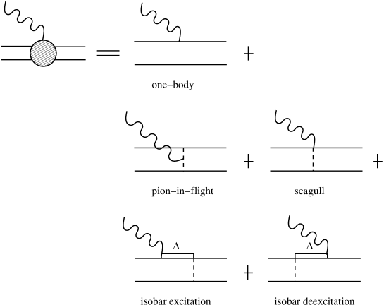
Figure 1: The electromagnetic current contributions taken into account in the present approach.

The nuclear current operator $\hat{j}^{\mu}(r)$ is the sum of a one- and a two-body part (see fig. 1). The one-body part consists of the usual charge operator and the convection and spin currents. In the present version of our model, the two-body part consists of the nonrelativistic pionic seagull MEC, the pion-in-flight MEC and the $\Delta$-contribution, whose explicit expressions can be found, for example, in Gui98 ; WiA97 . Note that the seagull and the pion-in-flight MEC do not contribute in pp-emission, at least in the adopted nonrelativistic limit.

The TOF requires a calculation of the two-hole spectral function including consistently different types of correlations, i.e. SRC and TC, as well as long-range correlations (LRC), mainly representing collective excitations of nucleons at the nuclear surface.

So far, different approaches are available in the most refined version of our model for pp- and pn-knockout Gui99 ; Gui97 . In both cases the TOF for transitions to discrete low-lying states of the residual nucleus are given by a combination of different components of the relative and center-of-mass (CM) motion. SRC and TC are introduced in the radial wave function of the relative motion by means of state dependent defect functions which are added to the uncorrelated partial wave. For the pp-case Gui97 ; Geu96 , the defect functions are obtained by solving the Bethe-Goldstone equation using, for a comparison, different NN-interactions: Bonn OBEPQ-A, Bonn OBEPQ-C Mac89 , and Reid Soft Core Reid . The calculations with the Bonn OBEPQ-A and Bonn OBEPQ-C potentials do not show significant differences, while those with the Reid Soft Core potential produce lower cross sections which are in worse agreement with the available $(e,e^{\prime}pp)$ data Gui97 ; Ond98 ; Ros00 ; Sta00 . For the pn-case Gui99 , SRC and TC correlations are calculated within the framework of the coupled-cluster method MuP00 with the AV14-potential WiS84 and using the so-called $S_{2}$ approximation, where only $1$-particle $1$-hole and $2$-particle $2$-hole excitations are included in the correlation operator. This method is an extension of the Bethe-Goldstone equation and takes into account, among other things and besides particle-particle ladders, also hole-hole ladders. These, however, turn out to be rather small in ${}^{16}O$ MuP00 , so that the two approaches are similar in the treatment of SRC. The advantage of the coupled-cluster method is that it provides directly correlated two-body wave functions MuP00 ; Gui99 . TC give an important contribution to pn-knockout, while their role is very small in pp-knockout.

LRC are included in the expansion coefficients of the TOF. For the pp-case, these coefficients are calculated in an extended shell-model basis within a dressed random phase approximation Gui97 ; Geu96 . For the pn-case, a simple configuration mixing calculation of the two-hole states in ${}^{16}O$ has been done and only $1p$-hole states are considered for transitions to the low-lying states of ${}^{14}N$ Gui99 .

In the scattering state, the two outgoing nucleons 1 and 2 and the residual nucleus B interact via the potential

$$V_{f}=V^{OP}(1)+V^{OP}(2)+V^{NN}(1,2),$$ (2)

where $V^{OP}(i)$ denotes the interaction between the nucleon $i$ and the residual nucleus. In our approach we use a complex phenomenological optical potential fitted to nucleon-nucleus scattering data, which contains a central, a Coulomb and a spin-orbit term Nad81 . In order to ensure some consistency in the treatment of the NN-interaction in the initial and final states, we have used the same NN-potential $V^{NN}$ as in the calculation of the TOF, i.e., the OBEPQ-A potential for pp- and the AV14-potential for pn-emission. The sensitivity of NN-FSI effects to the choice of the potential is however small in the calculations.

In general, a consistent treatment of the final state would require a genuine three-body approach, that, due to the complexity of the problem, has never been realized till now for complex nuclei. Different approximations have been used in the past.

In the simplest picture, any interaction between the two nucleons and the residual nucleus is neglected, i.e. $V_{f}\equiv 0$, and a plane-wave approximation (PW) is assumed for the outgoing nucleon wave functions. If $\vec{p}^{\,\,0}_{i}$, $i\in\{1,2\}$, denotes the asymptotic momentum of the outgoing nucleon $i$ in the chosen reference frame, the corresponding state is therefore given by

$$\mbox{$|\psi_{f}\rangle$}^{PW}=\mbox{$|\vec{p}^{\,\,0}_{1}\rangle$}\,\mbox{$|\vec{p}^{\,\,0}_{2}\rangle$}\,\,,$$ (3)

where $|\vec{p}^{\,\,0}_{i}\rangle$ describes the plane-wave state of the nucleon $i$ with momentum $\vec{p}^{\,\,0}_{i}$.

In a more sophisticated approach, only the optical potential $V^{OP}(i)$ is considered while the mutual NN-interaction $V^{NN}(1,2)$ is neglected. In this so-called “distorted wave” (DW) approximation, which has commonly been used in our previous work, the final state is in general given by

$$\mbox{$|\psi_{f}\rangle$}^{DW}=\left(1+G_{0}(z)T^{OP}(z)\right)\mbox{$|\vec{p}^{\,\,0}_{1}\rangle$}\,\mbox{$|\vec{p}^{\,\,0}_{2}\rangle$}\,\,,$$ (4)

with

$$z=\frac{(\vec{p}^{\,\,0}_{1})^{2}}{2m_{1}}+\frac{(\vec{p}^{\,\,0}_{2})^{2}}{2m_{2}}+\frac{(\vec{p}_{B})^{2}}{2m_{B}}-i\epsilon\,\,.$$ (5)

In (4) $m_{i}$ denotes the mass of the nucleon $i$ and $\vec{p}_{B}$ is the asymptotic momentum of the residual nucleus, with mass $m_{B}$, that in the laboratory frame is given by

$$\vec{q}=\vec{p}^{\,\,0}_{1}+\vec{p}^{\,\,0}_{1}+\vec{p}_{B}\,\,.$$ (6)

The quantity

$$G_{0}(z)=\frac{1}{z-H_{0}(1)-H_{0}(2)-H_{0}(A-2)}$$ (7)

in (4) denotes the free three-body propagator, where the kinetic Hamiltonian $H_{0}$ is treated nonrelativistically excluding rest masses. The scattering amplitude $T^{OP}$ in (4) is in general given by the Lippmann-Schwinger equation, i.e.,

$$T^{OP}(z) = \left(V^{OP}(1)+V^{OP}(2)\right)+\left(V^{OP}(1)+V^{OP}(2)\right)G_{0}(z)T^{OP}(z)\,\,.$$ (8)

The residual nucleus has a rather large mass in comparison with the nucleon and can thus be considered as infinitely heavy. This is a good approximation, which considerably simplifies the calculation of the scattering state, that can thus be expressed in this limit as the product of two uncoupled single-particle distorted wave functions, i.e.,

$$\mbox{$|\psi_{f}\rangle$}^{DW}=\mbox{$|\phi^{OP}(\vec{p}^{\,\,0}_{1})\rangle$}\,\mbox{$|\phi^{OP}(\vec{p}^{\,\,0}_{2})\rangle$},$$ (9)

where $|\phi^{OP}(\vec{p}^{\,\,0}_{i})\rangle$, is given by

$$\mbox{$|\phi^{OP}(\vec{p}^{\,\,0}_{i})\rangle$}=\left(1+g^{i}_{0}(z_{i})t^{OP,i}(z_{i})\right)\mbox{$|\vec{p}^{\,\,0}_{i}\rangle$},$$ (10)

and

$$z_{i} = \frac{(\vec{p}^{\,\,0}_{i})^{2}}{2m_{i}}-i\epsilon\,\,,$$ (11)

$$g^{i}_{0}(z_{i}) = \frac{1}{z_{i}-H_{0}(i)}\,\,,$$ (12)

$$t^{OP,i}(z_{i}) = V^{OP}(i)+V^{OP}(i)g^{i}_{0}(z_{i})t^{OP,i}(z_{i})\,\,.$$ (13)

are the single-particle counterparts to (5), (7),(8), respectively. Equation (10) is equivalent to the single-particle Schrödinger equation

$$\left(H_{0}(i)+V^{OP}(i)\right)\mbox{$|\phi^{OP}(\vec{p}^{\,\,0}_{i})\rangle$}=\frac{(\vec{p}^{\,\,0}_{i})^{2}}{2m_{i}}\mbox{$|\phi^{OP}(\vec{p}^{\,\,0}_{i})\rangle$}$$ (14)

which is solved in our treatment numerically in configuration space.

In all previous works, but in our recent paper ScB03 , the interaction $V^{NN}$ between the two outgoing nucleons (NN-FSI) has been completely neglected. If we want to incorporate it in a fully consistent frame, an infinite series of contributions has to be taken into account in $T^{OP}$ and in the NN-scattering amplitude

$$t^{NN}(z_{12})=V^{NN}+V^{NN}g^{12}_{0}(z_{12})t^{NN}(z_{12}),$$ (15)

where $z_{12}=z_{1}+z_{2}$, and

$$g^{12}_{0}(z_{12})=\frac{1}{z_{12}-H_{0}(1)-H_{0}(2)}\,\,.$$ (16)

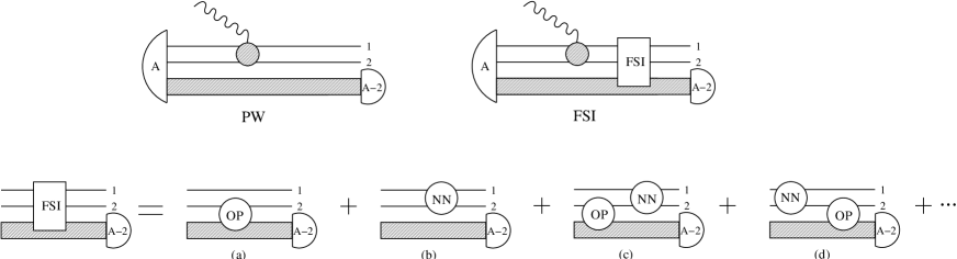
Figure 2: The relevant diagrams for electromagnetic two-nucleon knockout on a complex nucleus A. The two diagrams on top depict the plane-wave approximation (PW) and the distortion of the two outgoing proton wave functions by final state interactions (FSI). Below, the relevant mechanisms of FSI are depicted in detail, where the open circle denotes either the nucleon-nucleus scattering amplitude (OP), see (13), or the nucleon nucleon-scattering amplitude (NN), see (15). Diagrams which are given by an interchange of nucleon 1 and 2 are not depicted. In the present approach, only diagrams (a) and (b) are taken into account.

Adopting again the approximation $m_{B}\rightarrow\infty$, the leading order terms in the scattering amplitudes are given by (see fig. 2)

$$|\psi_{f}\rangle = \left(1+g^{12}_{0}(z_{12})t^{OP,12}(z_{12})+g^{12}_{0}(z_{12})t^{NN}(z_{12})+g^{12}_{0}(z_{12})t^{OP,12}(z_{12})g^{12}_{0}(z_{12})t^{NN}(z_{12})+\right.$$ (17)

$$\left.\,\,\,\,\,\,\,\,\,g^{12}_{0}(z_{12})t^{NN}(z_{12})g^{12}_{0}(z_{12})t^{OP,12}(z_{12})+...\right)\mbox{$|\vec{p}^{\,\,0}_{1}\rangle$}\,\mbox{$|\vec{p}^{\,\,0}_{2}\rangle$}\,\,,$$

where $t^{OP,12}(z_{12})$ follows from (8) with the substitution

$$G_{0}(z)\rightarrow g^{12}_{0}(z_{12})\,\,.$$ (18)

A consistent treatment of FSI would require a genuine three-body approach, with the usual computational challenges, by summing up the infinite series (17). We intend to tackle this project in the near future. At the moment, following the same approach as in ScB03 , we restrict ourselves to a perturbative treatment by taking into account only the first three terms in (17), i.e. the plane wave contribution and diagrams (a) and (b) in fig. 2. Formally, this corresponds to a perturbative treatment of $t^{OP,12}$ and $t^{NN}$ up to first order and where multiscattering processes, like the fourth and fifth terms in (17) (diagrams (c) and (d) in fig. 2), are neglected. Such an approximated but much more feasible treatment should allow us to study at least the main features of NN-FSI. In particular, it should allow us to answer the open question whether the neglect of NN-FSI in previous calculations can in general be justified or not. The present treatment of incorporating NN-FSI is denoted as DW-NN. We denote as PW-NN the treatment where only $V^{NN}$ is considered and $V^{OP}$ is switched off.

We would like to add that in practice the finite mass $m_{B}$ of the residual nucleus is taken into account in the PW- and DW-calculations by performing in (14) the transformation Gui91 ($i\neq j$)

$$\vec{p}^{\,\,0}_{i}\rightarrow\vec{q}^{\,\,0}_{i}=\frac{1}{m_{{}^{16}O}}\left[(m_{j}+m_{B})\vec{p}^{\,\,0}_{i}-m_{i}(\vec{p}^{\,\,0}_{j}+\vec{p}_{B})\right],$$ (19)

where $m_{{}^{16}O}$ denotes the mass of the ${}^{16}O$-target. Moreover, a semirelativistic generalization of (14) has been used as discussed in Nad81 .

In conclusion, the corresponding final states in the different approximations are given by

$$\mbox{$|\psi_{f}\rangle$}^{PW} = \mbox{$|\vec{q}^{\,\,0}_{1}\rangle$}\,\mbox{$|\vec{q}^{\,\,0}_{2}\rangle$}\,\,,$$ (20)

$$\mbox{$|\psi_{f}\rangle$}^{DW} = \mbox{$|\phi^{OP}(\vec{q}^{\,\,0}_{1})\rangle$}\,\mbox{$|\phi^{OP}(\vec{q}^{\,\,0}_{2})\rangle$}\,\,,$$ (21)

$$\mbox{$|\psi_{f}\rangle$}^{PW-NN} = \mbox{$|\vec{q}^{\,\,0}_{1}\rangle$}\,\mbox{$|\vec{q}^{\,\,0}_{2}\rangle$}+g^{12}_{0}(z_{12})t^{NN}(z_{12})\mbox{$|\vec{p}^{\,\,0}_{1}\rangle$}\,\mbox{$|\vec{p}^{\,\,0}_{2}\rangle$}\,\,,$$ (22)

$$\mbox{$|\psi_{f}\rangle$}^{DW-NN} = \mbox{$|\phi^{OP}(\vec{q}^{\,\,0}_{1})\rangle$}\,\mbox{$|\phi^{OP}(\vec{q}^{\,\,0}_{2})\rangle$}+g^{12}_{0}(z_{12})t^{NN}(z_{12})\mbox{$|\vec{p}^{\,\,0}_{1}\rangle$}\,\mbox{$|\vec{p}^{\,\,0}_{2}\rangle$}\,\,.$$ (23)

III Numerical treatment of NN-FSI

In general, we intend to be as flexible as possible in the treatment of NN-FSI. Consequently, we use the momentum and not the configuration space for the evaluation of the scattering amplitude $t^{NN}(z_{12})$ in (15), so that also nonlocal potentials, like the Bonn OBEPQ-A potential, which is used in Gui99 ; Geu96 to calculate the defect functions of the pp-case, can be considered. Moreover, in momentum space it is much easier to incorporate in the NN-FSI also the $\Delta$-isobar consistently within a coupled-channel approach ScA01 . Due to the rather large energies of the real or virtual photon in the kinematics discussed below, it cannot be excluded from the beginning that this contribution can be neglected in the NN-FSI. In forthcoming studies we intend to investigate this question in some detail. In the present paper, however, we restrict ourselves to the genuine NN-potential AV14 for pn- and the Bonn OBEPQ-A potential for pp-emission.

Since both the electromagnetic current and the TOF are calculated in the model in the configuration space, we have to adopt a suitable Fourier transformation of the relative coordinatesGui91 $\vec{r}_{1B}=\vec{r}_{1}-\vec{r}_{B}$ and $\vec{r}_{2B}=\vec{r}_{2}-\vec{r}_{B}$ of the three-body system. Taking into account the CM correction (19), we have therefore to evaluate

$$\langle\psi_{f}|\vec{r}_{1B},\vec{r}_{2B}\rangle \equiv \mbox{$\langle\psi_{f}(\vec{p}_{1}^{\,\,0},\vec{p}_{2}^{\,\,0})|\vec{r}_{1B},\vec{r}_{2B}\rangle$}=\mbox{$\langle\phi^{OP}(\vec{q}_{1}^{\,\,0})|\vec{r}_{1B}\rangle$}\,\,\mbox{$\langle\phi^{OP}(\vec{q}_{2}^{\,\,0})|\vec{r}_{2B}\rangle$}\,\,+$$ (24)

$$\,\,\,\int d^{3}p_{1}d^{3}p_{2}\mbox{$\langle\vec{p}_{1}^{\,\,0},\vec{p}_{2}^{\,\,0}|$}\,\,t^{NN}(z_{12}^{\ast})\,\,g^{12}_{0}(z_{12}^{\ast})\mbox{$|\vec{p}_{1},\vec{p}_{2}\,\rangle$}\mbox{$\langle\vec{p}_{1}|\vec{r}_{1B}\rangle$}\,\mbox{$\langle\vec{p}_{2}|\vec{r}_{2B}\rangle$}\,\,.$$

Note that the final state is completely determined by the asymptotic momenta $\vec{p}_{1}^{\,\,0}$ and $\vec{p}_{2}^{\,\,0}$ of the two nucleons, while the recoil momentum of the residual nucleus $\vec{p}_{\rm B}$ is given by Eq. (6). Additional spin and isospin quantum numbers are suppressed at the moment for the sake of simplicity.

The 6-dimensional integral in (24) can be reduced to a 3-dimensional one by exploiting in $t^{NN}$ the conservation of the total momentum of the two nucleons, i.e.,

$$\mbox{$\langle\vec{p}_{1}^{\,\,\prime},\vec{p}_{2}^{\,\,\prime}|$}\,\,t^{NN}(z_{12}^{\ast})\mbox{$|\vec{p}_{1},\vec{p}_{2}\,\rangle$}=\delta^{(3)}\left(\vec{p}_{1}^{\,\,\prime}+\vec{p}_{2}^{\,\,\prime}-\vec{p}_{1}-\vec{p}_{2}\right)\mbox{$\langle\frac{\vec{p}_{1}^{\,\,\prime}-\vec{p}_{2}^{\,\,\prime}}{2}|$}\,\,t^{NN}(z_{12}^{\ast})\mbox{$|\frac{\vec{p}_{1}-\vec{p}_{2}}{2}\rangle$}\,\,.$$ (25)

After some straightforward algebra one obtains

$$\langle\psi_{f}(\vec{p}_{1}^{\,\,0},\vec{p}_{2}^{\,\,0})|\vec{r}_{1B},\vec{r}_{2B}\rangle = \mbox{$\langle\phi^{OP}(\vec{q}_{1}^{\,\,0})|\vec{r}_{1B}\rangle$}\,\,\mbox{$\langle\phi^{OP}(\vec{q}_{2}^{\,\,0})|\vec{r}_{2B}\rangle$}\,\,+$$ (26)

$$\!\!\!\!\!\!\!\!\!\!\!\!\!\!\!\!\!\!\!\!\!\!\!\!\!\!\!\!\!\!\!\!\!\!\!\!\!\!\!\!\!\!\!\!\!\!\!\!\!\!\!\!\!\!\!\!\!\!\!\!\!\!\!\!\!\!\left(2\pi\right)^{-3}\,\,e^{-i\frac{\left(\vec{p}_{1}^{\,\,0}+\vec{p}_{2}^{\,\,0}\right)}{2}\cdot\left(\vec{r}_{1B}+\vec{r}_{2B}\right)}\int d^{3}p\mbox{$\langle\vec{p}_{rel}^{\,\,0}|$}\,\,t^{NN}({p}_{rel}^{0})\mbox{$|\vec{p}\,\rangle$}\frac{1}{\frac{\left({p}_{rel}^{0}\right)^{2}}{m_{N}}-\frac{p^{2}}{m_{N}}+i\epsilon}e^{-i\vec{p}\cdot\left(\vec{r}_{1B}-\vec{r}_{2B}\right)},$$

where the notation $p\equiv\left|\vec{p}\,\right|$ for any vector $\vec{p}$ is used, and

$$\vec{p}_{rel}^{\,\,0}=\frac{\vec{p}_{1}^{\,\,0}-\vec{p}_{2}^{\,\,0}}{2}$$ (27)

is the relative momentum of the two outgoing nucleons. Due to the fact that the Coulomb force is not incorporated in the NN-potential, we use in the propagator of (26) an average value for the nucleon mass, i.e.. $m_{1}=m_{2}\equiv m_{N}=938.926$ MeV. Moreover, we note that the states in the matrix element $t^{NN}(z_{12}^{\ast})\equiv t^{NN}({p}_{rel}^{0})$ of (25) and (26) correspond only to the relative motion of the two nucleons. In detail, the scattering amplitude in momentum space is given by the following integral equation

$$\mbox{$\langle\vec{p}^{\,\,\prime}|$}\,t^{NN}({p}_{rel}^{0})\mbox{$|\vec{p}\,\rangle$} = \mbox{$\langle\vec{p}^{\,\,\prime}|$}\,V_{NN}\mbox{$|\vec{p}\,\rangle$}\,+\,\int d^{3}k\mbox{$\langle\vec{p}^{\,\,\prime}|$}\,V_{NN}\mbox{$|\vec{k}\,\rangle$}\frac{1}{\frac{\left({p}_{rel}^{0}\right)^{2}}{M_{N}}-\frac{k^{2}}{M_{N}}+i\epsilon}\mbox{$\langle\vec{k}\,|$}\,t^{NN}({p}_{rel}^{0})\mbox{$|\vec{p}\,\rangle$}\,\,,$$

which can be solved with standard numerical methods ScZ74 ; Glo83 . Further details are given below.

In practice, (26) is exploited by using a partial wave decomposition. We must consider at this point that also the spin and isospin quantum numbers must be given for the outgoing particles. This means that the final state $|\psi_{f}\rangle$, which we have specified till now only by

$$\mbox{$|\psi_{f}\rangle$}\equiv\mbox{$|\psi_{f}(\vec{p}_{1}^{\,\,0},\vec{p}_{2}^{\,\,0})\rangle$}\,\,,$$ (29)

must be extended as

$$\mbox{$|\psi_{f}\rangle$}\equiv\mbox{$|\psi_{f}(\vec{p}_{1}^{\,\,0},\vec{p}_{2}^{\,\,0};s\,m_{s},t\,t_{0};\beta)\rangle$}\,\,.$$ (30)

Here, $s$ denotes the total spin of the two outgoing nucleons, with projection $m_{s}$ on their relative momentum $\vec{p}_{rel}^{\,\,0}$ (see (27)), $t$ the total isospin of the two nucleons, with third component $t_{0}$, and $\beta$ includes the spin and isospin quantum numbers of the residual nucleus state as well as its excitation energy.

Due to the fact that our chosen reference frame $\Sigma_{q}$ has the photon momentum $\vec{q}$ as quantization axis, one has to perform at first an (active) rotation of the spin state:

$$\langle sm_{s}| = \sum_{a}D^{[s]}_{m_{s}a}(0,-\Theta,-\Phi)\mbox{$\langle sa|$},$$ (31)

where $\Theta$ and $\Phi$ denote the polar angles of $\vec{p}_{rel}^{\,\,0}$ in $\Sigma_{q}$ and the rotation matrices can be found in Mes61 . Concerning the optical potential wave functions, $\langle\phi(\vec{q}_{1}^{\,\,0})|\vec{r}_{1B}\rangle$ and $\langle\phi(\vec{q}_{2}^{\,\,0})|\vec{r}_{2B}\rangle$ in (26), an uncoupled basis for the spin of the nucleons is appropriate. It is therefore useful to rewrite (31) as follows:

$$\langle sm_{s}| = \sum_{a,s_{1},s_{2}}D^{[s]}_{m_{s}a}(0,-\Theta,-\Phi)\mbox{$\langle\frac{1}{2}s_{1}\frac{1}{2}s_{2}|sa\rangle$}\mbox{$\langle\frac{1}{2}s_{1}|$}\,\mbox{$\langle\frac{1}{2}s_{2}|$}\,\,.$$ (32)

Note that the projection numbers $a,s_{1}$ and $s_{2}$ now refer to the reference frame $\Sigma_{q}$, with the photon momentum $\vec{q}$ along the $z$-axis, and $s_{1}$ ($s_{2}$) is the spin projection of nucleon 1 (2) in $\Sigma_{q}$. Inserting now spin and isospin degrees of freedom into (26), we obtain

$$\langle\psi_{f}|\vec{r}_{1B},\vec{r}_{2B}\rangle \equiv \langle\psi_{f}(\vec{p}_{1}^{\,\,0},\vec{p}_{2}^{\,\,0};s\,m_{s},t\,t_{0};\beta)|\vec{r}_{1B},\vec{r}_{2B}\rangle$$

$$\!\!\!\!\!\!\!\!\!\!\!\!\!\!\!\!\!\!\!\!\!\!\!\!\!\!\!\!\!\!\!\!\!\!\!\!\!\!\!\!\!\!\!\!=\sum_{a,s_{1},s_{2}}\sum_{t_{1},t_{2}}\sum_{s^{\prime}_{1},s^{\prime}_{2}}\sum_{t^{\prime}_{1},t^{\prime}_{2}}D^{[s]}_{m_{s}a}(0,-\Theta,-\Phi)\mbox{$\langle\frac{1}{2}s_{1}\frac{1}{2}s_{2}|sa\rangle$}\mbox{$\langle\frac{1}{2}t_{1}\frac{1}{2}t_{2}|tt_{0}\rangle$}\,\,\times$$

$$\!\!\!\!\!\!\!\!\!\!\!\!\!\!\!\!\!\!\!\!\!\!\!\!\!\!\!\!\!\!\!\!\!\!\!\!\!\!\!\!\!\!\!\!\mbox{$\langle\phi(\vec{q}_{1}^{\,\,0},s_{1}s^{\prime}_{1},t_{1}t^{\prime}_{1};\beta)|\vec{r}_{1B}\rangle$}\,\,\mbox{$\langle\phi(\vec{q}_{2}^{\,\,0},s_{2}s^{\prime}_{2},t_{2}t^{\prime}_{2};\beta)|\vec{r}_{2B}\rangle$}\,\,\,\,\mbox{$\langle\frac{1}{2}s^{\prime}_{1}|$}\,\,\mbox{$\langle\frac{1}{2}s^{\prime}_{2}|$}\,\,\mbox{$\langle\frac{1}{2}t^{\prime}_{1}|$}\,\,\mbox{$\langle\frac{1}{2}t^{\prime}_{2}|$}+$$

$$\!\!\!\!\!\!\!\!\!\!\!\!\!\!\!\!\!\!\!\!\!\!\!\!\!\!\!\!\!\!\!\!\!\!\!\!\!\!\!\!\!\!\!\!\left(2\pi\right)^{-3}\,\,e^{-i\frac{\left(\vec{p}_{1}^{\,\,0}+\vec{p}_{2}^{\,\,0}\right)}{2}\cdot\left(\vec{r}_{1B}+\vec{r}_{2B}\right)}\int d^{3}p\mbox{$\langle\vec{p}_{rel}^{\,\,0},s\,m_{s},t\,t_{0}|$}\,\,T_{NN}({p}_{rel}^{0})\mbox{$|\vec{p}\,\rangle$}\frac{1}{\frac{\left({p}_{rel}^{0}\right)^{2}}{M_{N}}-\frac{p^{2}}{M_{N}}+i\epsilon}e^{-i\vec{p}\cdot\left(\vec{r}_{1b}-\vec{r}_{2B}\right)}\,\,,$$

where the distorted wave function $\langle\phi(\vec{q}_{i}^{\,\,0},s_{i},s^{\prime}_{i},t_{i},t^{\prime}_{i};\beta)|\vec{r}_{i3}\rangle$ with spin and isospin projection numbers $s_{i},s^{\prime}_{i},t_{i},t^{\prime}_{i}$ is given by (consider (10))

$$\mbox{$\langle\phi(\vec{q}_{i}^{\,\,0},s_{i},s^{\prime}_{i},t_{i},t^{\prime}_{i};\beta)|\vec{r}_{i3}\rangle$}=\mbox{$\langle\vec{q}_{i}^{\,\,0},s_{i},t_{i};\beta|$}\left(1+t^{OP,i}(z^{\ast}_{i})g_{0}^{i}(z^{\ast}_{i})\right)\mbox{$|\vec{r}_{i3},s^{\prime}_{i},t^{\prime}_{i}\rangle$}\,\,.$$ (34)

In order to exploit (LABEL:final6), we use the following identities:

• partial wave decomposition of a plane wave:

$$e^{i\vec{a}\cdot\vec{b}}=4\pi\sum_{l,m}i^{l}j_{l}(ab)\left(Y^{[l]}_{m}(\hat{a})\right)^{\ast}Y^{[l]}_{m}(\hat{b}),$$ (35)

where $j_{l}$ denote the spherical Bessel functions;

• partial wave decomposition of $\langle\vec{p}_{rel}^{\,\,0},s\,m_{s}|$ in (LABEL:final6):

  $$\mbox{$\langle\vec{p}_{rel}^{\,\,0},s\,m_{s}|$}=\frac{1}{\sqrt{4\pi}}\sum_{ljm}\sqrt{2l+1}\mbox{$\langle l0sm_{s}|jm_{s}\rangle$}D^{[j]}_{m_{s}m}(0,-\Theta,-\Phi)\mbox{$\langle p^{0}_{rel}(ls)jm|$}\,\,,$$ (36)

  where the projection $m$ refers to the $z$-axis of $\Sigma_{q}$;

• partial wave decomposition of a state $|\vec{p}\,\rangle$

  $$\langle\vec{p}\,|(q(ls)jm,tt_{0})\rangle = \frac{1}{p^{2}}\delta(p-q)\left[Y^{[l]}(\hat{p})\times\left[\chi^{[\frac{1}{2}]}(1)\times\chi^{[\frac{1}{2}]}(2)\right]^{[s]}\right]^{[j]}_{m}\,\,\mbox{$|\frac{1}{2}\frac{1}{2}tt_{0}\rangle$}\,\,,$$ (37)

  where $\chi^{[\frac{1}{2}]}(i)$ denotes the Pauli-spinor of nucleon $i$.

• For the matrix element of the $NN$-scattering amplitude between partial waves, one can exploit the fact that $t^{NN}$ is a rank-0 tensor operator:

  $$\mbox{$\langle p^{\prime}(l^{\prime}s^{\prime})j^{\prime}m^{\prime},t^{\prime}t_{0}^{\prime}|$}t^{NN}(p^{0}_{rel})\mbox{$|p(ls)jm,tt_{0}\rangle$}=\delta_{jj^{\prime}}\delta_{mm^{\prime}}\delta_{tt^{\prime}}\delta_{t_{0}t_{0}^{\prime}}\delta_{s^{\prime}s}t^{j\,s\,t}(p^{\prime}l^{\prime},pl;p^{0}_{rel})\,\,.$$ (38)

  The quantity $t^{j\,s\,t}(p^{\prime}l^{\prime},pl;p^{0}_{rel})$ is given by a 1-dimensional integral equation which can be derived from (LABEL:tnn_2). With the help of Gaussian mesh points, the latter can be transformed into a matrix equation which is solved directly by matrix inversion Sch99 .

With the help of these relations, one obtains, after some straightforward algebra, the following final result:

$$\langle\psi_{f}|\vec{r}_{1B},\vec{r}_{2B}\rangle \equiv \langle\psi_{f}(\vec{p}_{1}^{\,\,0},\vec{p}_{2}^{\,\,0};s\,m_{s},t\,t_{0};\beta)|\vec{r}_{1B},\vec{r}_{2B}\rangle$$ (39)

$$\!\!\!\!\!\!\!\!\!\!\!\!\!\!\!\!\!\!\!\!\!\!\!\!\!\!\!\!\!\!\!\!\!\!\!\!\!\!\!\!\!\!\!\!=\,\,\sum_{a,s_{1},s_{2}}\sum_{t_{1},t_{2}}\sum_{s^{\prime}_{1},s^{\prime}_{2}}\sum_{t^{\prime}_{1},t^{\prime}_{2}}D^{[s]}_{m_{s}a}(0,-\Theta,-\Phi)\mbox{$\langle\frac{1}{2}s_{1}\frac{1}{2}s_{2}|sa\rangle$}\mbox{$\langle\frac{1}{2}t_{1}\frac{1}{2}t_{2}|tt_{0}\rangle$}\,\,\times$$

$$\!\!\!\!\!\!\!\!\!\!\!\!\!\!\!\!\!\!\!\!\!\!\!\!\!\!\!\!\!\!\!\!\!\!\!\!\!\!\!\!\!\!\!\!\mbox{$\langle\phi(\vec{q}_{1}^{\,\,0},s_{1}s^{\prime}_{1},t_{1}t^{\prime}_{1};\beta)|\vec{r}_{1B}\rangle$}\,\,\mbox{$\langle\phi(\vec{q}_{2}^{\,\,0},s_{2}s^{\prime}_{2},t_{2}t^{\prime}_{2};\beta)|\vec{r}_{2B}\rangle$}\,\,\,\,\mbox{$\langle\frac{1}{2}s^{\prime}_{1}|$}\,\,\mbox{$\langle\frac{1}{2}s^{\prime}_{2}|$}\,\,\mbox{$\langle\frac{1}{2}t^{\prime}_{1}|$}\,\,\mbox{$\langle\frac{1}{2}t^{\prime}_{2}|$}+$$

$$\!\!\!\!\!\!\!\!\!\!\!\!\!\!\!\!\!\!\!\!\!\!\!\!\!\!\!\!\!\!\!\!\!\!\!\!\!\!\!\!\!\!\!\!\left(2\pi\right)^{-3}\,\,e^{-i\frac{\left(\vec{p}_{1}^{\,\,0}+\vec{p}_{2}^{\,\,0}\right)}{2}\cdot\left(\vec{r}_{1B}+\vec{r}_{2B}\right)}\sum_{s^{\prime}_{1},s^{\prime}_{2}}\sum_{t^{\prime}_{1},t^{\prime}_{2}}\sum_{l^{\prime},n_{1},n_{2}}\sqrt{4\pi}F_{l^{\prime},n_{1},n_{2}}(\left|\vec{r}_{1B}-\vec{r}_{2B}\right|,p^{0}_{rel},sm_{s},t)\,\,\times$$

$$\!\!\!\!\!\!\!\!\!\!\!\!\!\!\!\!\!\!\!\!\!\!\!\!\!\!\!\!\!\!\!\!\!\!\!\!\!\!\!\!\!\!\!\!Y^{[l^{\prime}]}_{-n_{1}}(\widehat{\vec{r}_{2B}-\vec{r}_{1B}})\,\,\mbox{$\langle\frac{1}{2}s^{\prime}_{1}\frac{1}{2}s^{\prime}_{2}|sn_{2}\rangle$}\mbox{$\langle\frac{1}{2}t^{\prime}_{1}\frac{1}{2}t^{\prime}_{2}|tt_{0}\rangle$}\,\,\mbox{$\langle\frac{1}{2}s^{\prime}_{1}|$}\,\,\mbox{$\langle\frac{1}{2}s^{\prime}_{2}|$}\,\,\mbox{$\langle\frac{1}{2}t^{\prime}_{1}|$}\,\,\mbox{$\langle\frac{1}{2}t^{\prime}_{2}|$}$$

where the function $F$ in (39) is given by

$$F_{l^{\prime},n_{1},n_{2}}(\left|\vec{r}_{1B}-\vec{r}_{2B}\right|,p^{0}_{rel},sm_{s},t) = \sum_{l,j}\int dpp^{2}i^{l^{\prime}}j_{l^{\prime}}(p\left|\vec{r}_{2B}-\vec{r}_{1B}\right|)(-1)^{n_{1}}\frac{1}{\frac{\left({p}_{rel}^{0}\right)^{2}}{M_{N}}-\frac{p^{2}}{M_{N}}+i\epsilon}$$ (40)

$$\!\!\!\!\!\!\!\!\!\!\!\!\!\!\!\!\!\!\!\!\!\!\!\!\!\!\!\!\!\!\!\!\!\!\!\!\!\!\!\!\!\!\!\!\!\!\!\!\!\!\!\!\!\!\!\!\!\!\!\!\!\!\!\!\!\!\!\!\!\!\!\!\!\!\!\!\!\!\sqrt{2l+1}\mbox{$\langle l0sm_{s}|jm_{s}\rangle$}D^{[j]}_{m_{s}n_{1}+n_{2}}(0,-\Theta,-\Phi)t^{j\,s\,t_{0}}(p^{\prime}l^{\prime},pl;p^{0}_{rel})\mbox{$\langle l^{\prime}n_{1}sn_{2}|jn_{1}+n_{2}\rangle$}\,\,.$$

In our explicit evaluation, we have taken an upper limit of $l^{\prime}=3$, i.e., we have considered the isospin-1 partial waves ${}^{1}\!S_{0},^{3}\!P_{0},^{3}\!P_{1},^{3}\!P_{2},^{1}\!D_{2},^{3}\!F_{2},^{3}\!F_{3}$, and ${}^{3}\!F_{4}$ for pp-knockout and in addition the isospin-0 contributions ${}^{3}\!S_{1},^{1}\!P_{1},^{3}\!D_{1},^{3}\!D_{2},^{3}\!D_{3}$, and ${}^{1}\!F_{3}$ for pn-knockout. Concerning the summation index $l$ in (40), the limit $l^{\prime}\leq 3$ implies that in addition also $l=4$ and $l=5$ contributions (${}^{3}\!G_{3}$ and ${}^{3}\!H_{4}$) are considered. It has been checked numerically that this truncation is sufficient at least for the kinematics considered in this paper.

IV Results

In this section, we discuss the role of NN-FSI on different electromagnetic reactions with pp- and pn-knockout from ${}^{16}O$. The case of the ${}^{16}O(e,e^{\prime}pp)^{14}C$ reaction has already been considered in ScB03 , where it has been found that the effects of NN-FSI depend on kinematics, on the different partial waves for the relative motion of the nucleon pair in the initial state and, therefore, on the final state of the residual nucleus. In particular, a considerable enhancement for medium and large values of the recoil momentum has been found, for the transition to the $0^{+}$ ground state of ${}^{14}C$, just in the superparallel kinematics of a recent experiment at MAMI Ros00 . Since similar kinematics has been proposed for the first ${}^{16}O(e,e^{\prime}pn)^{14}N$ experiment at MAMI Arn98 , this is the first case we have considered in the present investigation.

The calculated differential cross sections of the ${}^{16}O(e,e^{\prime}pp)$ reaction to the $0^{+}$ ground state of ${}^{14}C$ and of the ${}^{16}O(e,e^{\prime}pn)$ reaction to the $1^{+}$ ground state of ${}^{14}N$ in superparallel kinematics are displayed in the left and right panels of fig. 3, respectively. The results given by the different approximations (20-23) are compared in the figure. The ${}^{16}O(e,e^{\prime}pp)^{14}C$ cross section was already presented in ScB03 and is shown again here only to allow a more direct comparison of FSI effects on pp- and pn-emission in the same kinematics.

It can be clearly seen in the figure that the inclusion of the optical potential leads, in both reactions, to an overall and substantial reduction of the calculated cross sections (see the difference between the PW and DW results). This effect is well known and it is mainly due to the imaginary part of the optical potential, that accounts for the flux lost to inelastic channels in the nucleon-residual nucleus elastic scattering. The optical potential gives the dominant contribution of FSI for recoil-momentum values up to $p_{\rm B}\simeq 150$ MeV/$c$. At larger values NN-FSI gives an enhancement of the cross section, that increases with $p_{\rm B}$. In $(e,e^{\prime}pp)$ this enhancement goes beyond the PW result and amounts to roughly an order of magnitude for $p_{\rm B}\simeq 300$ MeV/$c$. In $(e,e^{\prime}pn)$ this effect is still sizeable but much weaker. We note that in both cases the contribution of NN-FSI is larger in the DW-NN than in the PW-NN approximation.

In order to understand NN-FSI effects in some more detail, the separated contributions of the different terms of the nuclear current in the DW and DW-NN approximations are compared in fig. 4 for pp- and in fig.  5 for pn-knockout. In $(e,e^{\prime}pp)$ NN-FSI produces a strong enhancement of the $\Delta$-current contribution for all the values of $p_{\rm B}$. Up to about 100-150 MeV/$c$, however, this effect is completely overwhelmed by the dominant contribution of the one-body current, while for larger values of $p_{\rm B}$, where the one-body current is less important in the cross section, the increase of the $\Delta$-current is responsible for the substantial enhancement in the final result of fig. 4. The effect of NN-FSI on the one-body current is much weaker but anyhow sizeable, and it is responsible for the NN-FSI effect at lower values of $p_{\rm B}$ in fig. 4.

We have found in a detailed analytical analysis that the antisymmetrization of the final NN-state leads to a strong suppression of the $\Delta$-current contribution if the momenta of the nucleons after the deexcitation of the $\Delta$ (consider fig.  1) are aligned parallel or antiparallel to the photon momentum $\vec{q}$. However, this situation is in general not present when NN-FSI are taken into account, even in superparallel kinematics.

Different effects of NN-FSI on the various components of the current are shown for the $(e,e^{\prime}pn)$ reaction in fig. 5. Also in this case, NN-FSI affects more the two-body than the one-body current. A sizeable enhancement is produced on the $\Delta$-current, at all the values of $p_{\rm B}$, and a huge enhancement on the seagull current at large momenta. In contrast, the one-body current is practically unaffected by NN-FSI up to about 150 MeV/$c$. A not very large but visible enhancement is produced at larger momenta, where, however, the one-body current gives only a negligible contribution to the final cross section. The role of the pion-in-flight term, in both DW and DW-NN approaches, is practically negligible in the cross section. Thus, a large effect is given by NN-FSI on the seagull and the $\Delta$-current. The sum of the two terms, however, produces a destructive interference that leads to a partial cancellation in the final cross section. The net effect of NN-FSI in fig. 3 is not large but anyhow non negligible. Moreover, the results for the partial contributions in fig. 5 indicate that in pn-knockout NN-FSI can be large in particular situations and therefore should in general be included in a careful evaluation.

The cross section of the ${}^{16}O(\gamma,pp)$ reaction to the $0^{+}$ ground state of ${}^{14}C$ calculated with the different approximations for FSI is shown in fig. 6. The separated contributions of the one-body and $\Delta$-currents in DW and DW-NN are displayed in fig. 7. Calculations have been performed in superparallel kinematics, and for an incident photon energy which has the same value, $E_{\gamma}=215$ MeV, as the energy transfer in the $(e,e^{\prime}pp)$ calculation of fig. 3. This kinematics, which is not very well suited for $(\gamma,pp)$ experiments, can be interesting for a theoretical comparison with the corresponding results of the electron induced reactions in figs. 3 and 4.

In general, two-body currents give the major contribution to $(\gamma,NN)$ reactions. In this superparallel kinematics, however, the $(\gamma,pp)$ cross section is dominated by the one-body current for recoil momentum values up to about 150 MeV/$c$. For larger values the $\Delta$-current plays the main role. This is the same behavior as in the corresponding situation for $(e,e^{\prime}pp)$. In fig. 7 NN-FSI produces a significant enhancement of the $\Delta$-current contribution, that, however, is not as large as in $(e,e^{\prime}pp)$. The role of NN-FSI on the one-body current is negligible in $(\gamma,pp)$, while it is significant in $(e,e^{\prime}pp)$. This effect is produced in $(e,e^{\prime}pp)$ on the longitudinal part of the nuclear current, that does not contribute in reactions induced by a real photon. Thus, in practice, in this kinematics NN-FSI affects only the $\Delta$-current and therefore in fig. 6 its effect is negligible in the region where the one-body current is dominant. At large values of $p_{\rm B}$, where the role of the $\Delta$-current becomes important, the enhancement produced by NN-FSI is sizeable, but weaker than in the same superparallel kinematics for $(e,e^{\prime}pp)$. We note that also for the $(\gamma,pp)$ reaction in fig. 6 NN-FSI effects are larger in the DW-NN than in the PW-NN approach.

Another example is presented in fig. 8, where the results of the different approximations in the treatment of FSI are displayed for the ${}^{16}O(\gamma,pp)$ reaction to the $0^{+}$ ground state of ${}^{14}C$ (left panel) and for the ${}^{16}O(\gamma,pn)$ reaction to the $1^{+}$ ground state of ${}^{14}N$ (right panel) in a coplanar kinematics at $E_{\gamma}=120$ MeV, where the energy and the scattering angle of the outgoing proton are fixed at $T_{1}=45$ MeV and $\gamma_{1}=45^{\circ}$, respectively. Different values of the recoil momentum can be obtained by varying the scattering angle $\gamma_{2}$ of the second outgoing nucleon on the other side of the photon momentum. It can be clearly seen in the figure that NN-FSI has almost no effect. In contrast, a very large contribution is given, for both reactions, by the optical potential, which produces a substantial reduction of the calculated cross sections. This kinematics, which appears within reach of available experimental facilities, was already envisaged in Gui01 as promising to study SRC in the $(\gamma,pp)$ reaction. In fact, at the considered value of the photon energy, the contribution of the $\Delta$-current is relatively much less important, and while the $(\gamma,pn)$ cross section is dominated by the seagull current Gui01 , in the $(\gamma,pp)$ cross section the contribution of the one-body current is large and competitive with the one of the two-body current. This can be seen in fig. 9, where the two separated contributions are shown in the DW and in the DW-NN approximations. Both processes are important: the $\Delta$-current plays the main role at lower values of $\gamma_{2}$, while for $\gamma_{2}\geq 110^{\circ}$ the one-body current and therefore SRC give the major contribution. The effect of NN-FSI is practically negligible on both terms, which explains the result in the final cross section of fig. 9.

A study of the $(\gamma,pp)$ reaction in a kinematics of the type considered in figs. 8 and 9, where NN-FSI is negligible and correlations are important, might represent a promising alternative to the $(e,e^{\prime}pp)$ reaction for the investigation of SRC.

V Summary and Outlook

The relevance of the mutual final state interaction of the two emitted nucleons (NN-FSI) in electro- and photoinduced two-nucleon knockout from ${}^{16}O$ has been investigated within a perturbative treatment.

A consistent evaluation of FSI would require a genuine three-body approach, for the two nucleons and the residual nucleus, by summing up an infinite series of contributions in the NN-scattering amplitude and in the interaction of the two nucleons with the residual nucleus. In all previous calculations performed till now on complex nuclei, apart from our recent paper ScB03 , NN-FSI was neglected and only the interaction of each of the two nucleons with the residual nucleus was included. In our model this effect is accounted for by a phenomenological optical potential. Following the same approach as in ScB03 , here NN-FSI has been incorporated in the model within a perturbative treatment of the optical potential and of the NN-interaction up to first order in the corresponding scattering amplitudes. Therefore, both effects of FSI, due to NN-FSI and to the optical potential, are taken into account in the present treatment, but the multiscattering processes, where the two effects are intertwined, are neglected. In spite of that, the most important part of both contributions is presumably included in the present treatment. Such an approximated but more feasible approach should therefore be able to give a reliable idea of the relevance of NN-FSI.

The full three-body approach, which represents a computationally challenging task, will anyhow be tackled in forthcoming studies, in order to give a more definite answer about the role of NN-FSI, especially in those situations where the effect turns out to be large in the present treatment.

Numerical results of cross sections calculated for different reactions and kinematics have been presented. In order to understand in more detail the role of the various effects of FSI, the results of the perturbative treatment, where both the optical potential and the NN-interaction are included, have been compared with the more approximated approaches where only either contribution is considered, as well as with the simplest calculations where FSI are completely neglected and the PW approximation is assumed for the outgoing nucleons.

In general, the optical potential gives an overall and substantial reduction of the calculated cross sections. This important effect represents the main contribution of FSI and can never be neglected. In most of the situations considered here, NN-FSI gives an enhancement of the cross section. The effect is in general non negligible, it depends strongly on the kinematics, on the type of reaction, and, as it is shown in ScB03 , on the final state of the residual nucleus. NN-FSI affects in a different way the various terms of the nuclear current, usually more the two-body than the one-body terms, and is sensitive to the various theoretical ingredients of the calculation. This makes it difficult to make predictions about the role of NN-FSI in a particular situation. In general each specific situation should be individually investigated.

The results obtained in the present investigation indicate that NN-FSI effects are in general larger in pp- than in pn-knockout and in electro- than in photoinduced reactions. In particular situations they can be negligible, e.g., in the ${}^{16}O(\gamma,pp)^{14}C$ and ${}^{16}O(\gamma,pn)^{14}N$ reactions for the coplanar kinematics at $E_{\gamma}=120$ MeV considered here. In particular situations they can be large, e.g. in the superparallel kinematics of the ${}^{16}O(e,e^{\prime}pp)^{14}C_{\rm g.s.}$ reaction, where NN-FSI leads to a strong enhancement of the cross section, up to about one order of magnitude at large values of the recoil momentum. A qualitatively similar but quantitatively much weaker effect is obtained, in the same kinematics, for the ${}^{16}O(e,e^{\prime}pn)^{14}N$ and ${}^{16}O(\gamma,pp)^{14}C$ reactions.

In general, NN-FSI is non negligible. In spite of that, the original guess, that justified its neglect in the past, i.e. that its contribution does not significantly change the main qualitative features of the theoretical results, is basically correct. But if we want to obtain more reliable quantitative results and to get more insight into the two-nucleon knockout process, for a more careful comparison with available as well as future data, NN-FSI must be included in the model.

In order to improve the reliability of the theoretical description of the two-nucleon knockout process, the full three-body problem of the final state has to be tackled in forthcoming studies. In that context, special emphasis has to be devoted to a more consistent treatment of the initial and the final state.

Acknowledgements

This work has partly been performed under the contract HPRN-CT-2000-00130 of the European Commission. Moreover, it has been supported by the Istituto Nazionale di Fisica Nucleare and by the Deutsche Forschungsgemeinschaft (SFB 443). Fruitful discussions with H. Arenhövel are gratefully acknowledged.

Figure 3: The differential cross section of the ${}^{16}O(e,e^{\prime}pp)$ reaction to the $0^{+}$ ground state of ${}^{14}C$ (left panel) and of the ${}^{16}O(e,e^{\prime}pn)$ reaction to the $1^{+}$ ground state of ${}^{14}N$ (right panel) in a superparallel kinematics with an incident electron energy $E_{0}=855$ MeV, an electron scattering angle $\theta_{e}=18^{\circ}$, energy transfer $\omega=215$ MeV and $q=316$ MeV/$c$. In ${}^{16}O(e,e^{\prime}pn)$ the proton is ejected parallel and the neutron antiparallel to $\vec{q}$. Different values of $p_{\rm B}$ are obtained changing the kinetic energies of the outgoing nucleons. Positive (negative) values of $p_{\rm B}$ refer to situations where ${\vec{p}}_{\rm B}$ is parallel (anti-parallel) to ${\vec{q}}$. Line convention: PW (dotted), PW-NN (dash-dotted), DW (dashed), DW-NN (solid).

Figure 4: The differential cross section of the ${}^{16}O(e,e^{\prime}pp)$ reaction to the $0^{+}$ ground state of ${}^{14}C$ in the same superparallel kinematics as in fig. 3. Line convention: DW with the $\Delta$-current (dotted), DW-NN with the $\Delta$-current (dash-dotted), DW with the one-body current (dashed), DW-NN with the one-body current (solid).

Figure 5: The differential cross section of the ${}^{16}O(e,e^{\prime}pn)$ reaction to the $1^{+}$ ground state of ${}^{14}N$ in the same superparallel kinematics as in fig. 3. Line convention in the left panel: DW with the $\Delta$-current (dotted), DW-NN with the $\Delta$-current (dash-dotted), DW with the one-body-part (dashed), DW-NN with the one-body-part (solid). Line convention in the right panel: DW with the pion-in-flight-current (dotted), DW-NN with the pion-in-flight–current (dash-dotted), DW with the seagull-current (dashed), DW-NN with the seagull-current (solid).

Figure 6: The differential cross section of the ${}^{16}O(\gamma,pp)$ reaction to the $0^{+}$ ground state of ${}^{14}C$ in superparallel kinematics at $E_{\gamma}=$ 215 MeV. Line convention as in fig.  3.

Figure 7: The differential cross section of the ${}^{16}O(\gamma,pp)$ reaction to the $0^{+}$ ground state of ${}^{14}C$ in the same kinematics as in fig. 6. Line convention as in fig.  4.

Figure 8: The differential cross section of the ${}^{16}O(\gamma,pp)$ reaction to the $0^{+}$ ground state of ${}^{14}C$ (left panel) and of the ${}^{16}O(\gamma,pn)$ reaction to the $1^{+}$ ground state of ${}^{14}N$ (right panel) as a function of the scattering angle $\gamma_{2}$ of the second outgoing nucleon in a coplanar kinematics with $E_{\gamma}=$ 120 MeV, $T_{1}=45$ MeV and $\gamma_{1}=45^{\circ}$. Line convention as in fig.  3.

Figure 9: The differential cross section of the ${}^{16}O(\gamma,pp)$ reaction to the $0^{+}$ ground state of ${}^{14}C$ in the same kinematics as in fig. 8. Line convention as in fig. 4.

References

- (1) H. Müther and A. Polls, Prog. Part. Nucl. Phys. 45, 243 (2000).
-
(2)
K. Gottfried, Nucl. Phys. 5, 557 (1958);
Ann. of Phys. 21, 29 (1963);
W. Czyz and K. Gottfried, Ann. of Phys. 21, 47 (1963). - (3) S. Boffi, C. Giusti, F. D. Pacati and M. Radici, Electromagnetic Response of Atomic Nuclei (Oxford Studies in Nuclear Physics, Clarendon Press, Oxford, 1996).
- (4) C. Giusti and F. D. Pacati, Nucl. Phys. A 641, 297 (1998).
- (5) C. Giusti, H. Müther, F. D. Pacati and M. Stauf, Phys. Rev. C 60, 054608 (1999).
- (6) C. Giusti, F. D. Pacati, K. Allaart, W. J. W. Geurts, W. H. Dickhoff and H. Müther, Phys. Rev. C 57, 1691 (1998).
- (7) C. Giusti and F. D. Pacati, Nucl. Phys. A 615, 373 (1997).
- (8) C. Giusti and F. D. Pacati, Phys. Rev. C 61, 054617 (2000).
- (9) C. Giusti and F. D. Pacati, Eur. Phys. J. A 12, 69 (2001).
- (10) J. Ryckebusch, W. van Nespen, D. Debruyne, Phys. Lett. B 441, 1 (1998).
- (11) J. Ryckebusch, V. Van der Sluys, K. Heyde, H. Holvoet, W. Van Nespen, M. Waroquier, M. Vanderhaeghen, Nucl. Phys. A 624, 581 (1997).
- (12) J. Ryckebusch, D. Debruyne, W. van Nespen, Phys. Rev. C 57, 1319 (1998).
- (13) L. J. H. M. Kester et al., Phys. Rev. Lett. 74, 1712 (1995).
- (14) C. J. G. Onderwater et al., Phys. Rev. Lett. 78, 4893 (1997).
- (15) C. J. G. Onderwater et al., Phys. Rev. Lett. 81, 2213 (1998).
- (16) G. Rosner, Prog. Part. Nucl. Phys. 44, 99 (2000).
- (17) R. Starink et al., Phys. Lett. B 474, 33 (2000).
- (18) C. Giusti and F. D. Pacati, Nucl. Phys. A 535, 573 (1991).
- (19) The A2-collaboration at MAMI, Proposal No.: A2/4-97; spokesperson: P. Grabmayr.
- (20) The A1-collaboration at MAMI, Proposal No.: A1/5-98; spokespersons: P. Grabmayr and G. Rosner.
- (21) D. Knödler and H. Müther, Phys. Rev. C 63, 044602 (2001).
- (22) M. Schwamb, S. Boffi, C. Giusti and F. D. Pacati, Eur. Phys. J. A 17, 7 (2003).
- (23) J. C. McGeorge et al., Phys. Rev. C 51, 1967 (1995).
- (24) Th. Lamparter et al., Z. Phys. A 355, 1 (1996).
- (25) J. D. McGregor et al., Phys. Rev. Lett. 80, 245 (1998).
- (26) D. P. Watts et al., Phys. Rev. C 62, 014616 (2000).
- (27) P. Wilhelm, H. Arenhövel, C. Giusti and F. D. Pacati, Z. Phys. A 359, 467 (1997).
- (28) W. J. W. Geurts, K. Allaart, W. H. Dickhoff and H. Müther, Phys. Rev. C 54, 114 (1996).
- (29) R. Machleidt, Adv. Nucl. Phys. 19, 189 (1989).
- (30) R. Reid, Ann. of Phys. 50, 411 (1968).
- (31) R. B. Wiringa, R. A. Smith and T. L. Ainsworth, Phys. Rev. C 29, 1207 (1984).
- (32) A. Nadasen et al., Phys. Rev. C 23, 1023 (1981).
- (33) M. Schwamb and H. Arenhövel, Nucl. Phys. A 690, 647 (2001).
- (34) E. W. Schmid and H. Ziegelmann, The Quantum Mechanical Three-Body Problem (Friedrich Vieweg & Sohn, Braunschweig, 1974).
- (35) W. Glöckle, The Quantum Mechanical Few Body Problem (Springer-Verlag Berlin, Heidelberg, New York, Tokyo, 1983).
- (36) A. Messiah, Quantum Mechanics, Volume 2 (North-Holland, Amsterdam, Oxford, New York, Tokyo, 1961).
- (37) M. Schwamb, PhD-thesis, Johannes-Gutenberg Universität Mainz, 1999.